The Water Implications of Greenhouse Gas Mitigation: Effects on Land Use, Land Use Change, and Forestry


Abstract
1. Introduction
2. Literature Based Findings on Mitigation and Water
2.1. AF Management
2.2. Land Use Change
2.3. Bioenergy
2.4. Technological Progress
3. Empirical Investigation on Mitigation and Water
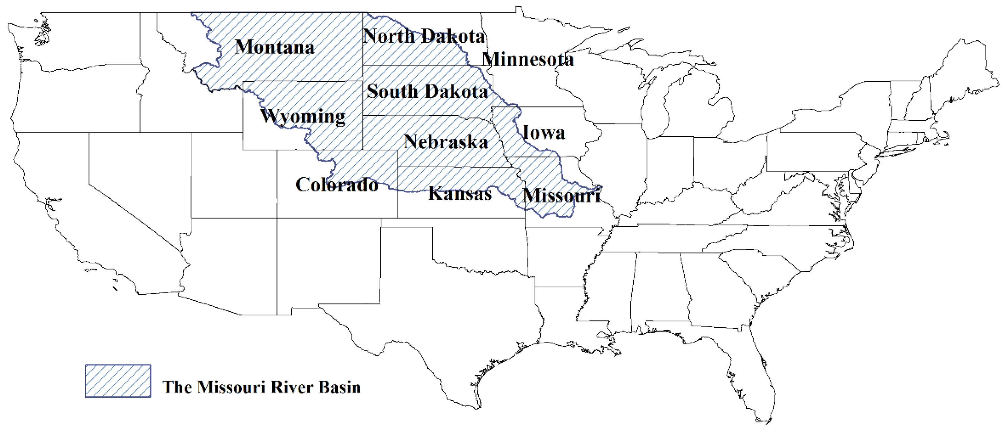
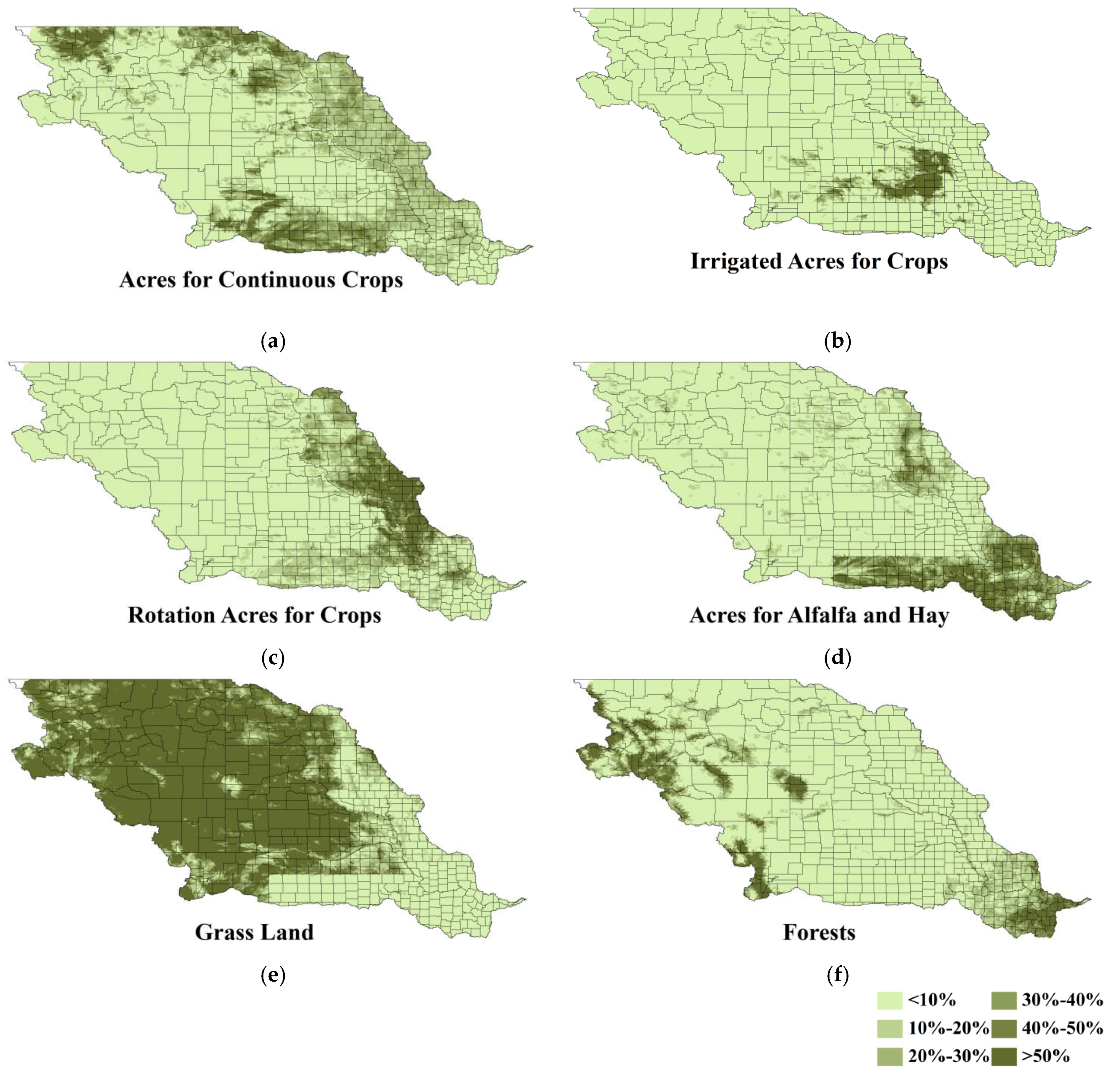
3.1. Study Area
3.2. SWAT Generated Data
- Total Nitrogen (N)
- Total Phosphorus (P)where and are the subindices for the nitrogen- and phosphorus-related measures. A single water quality index (WQI) is then formed from these subindices by using the unweighted harmonic square mean, as in Swamee and Tyagi [82]:where is the water quality index, is the number of subindices, and is the ith subindex.
3.3. Climatic Data
4. Methods
4.1. Quantile Regression over Panel Data
4.2. FASOMGHG Model
5. Estimation Results
5.1. Quantile Regression Results for Water Quantity
5.2. Quantile Regression Results for Water Quality
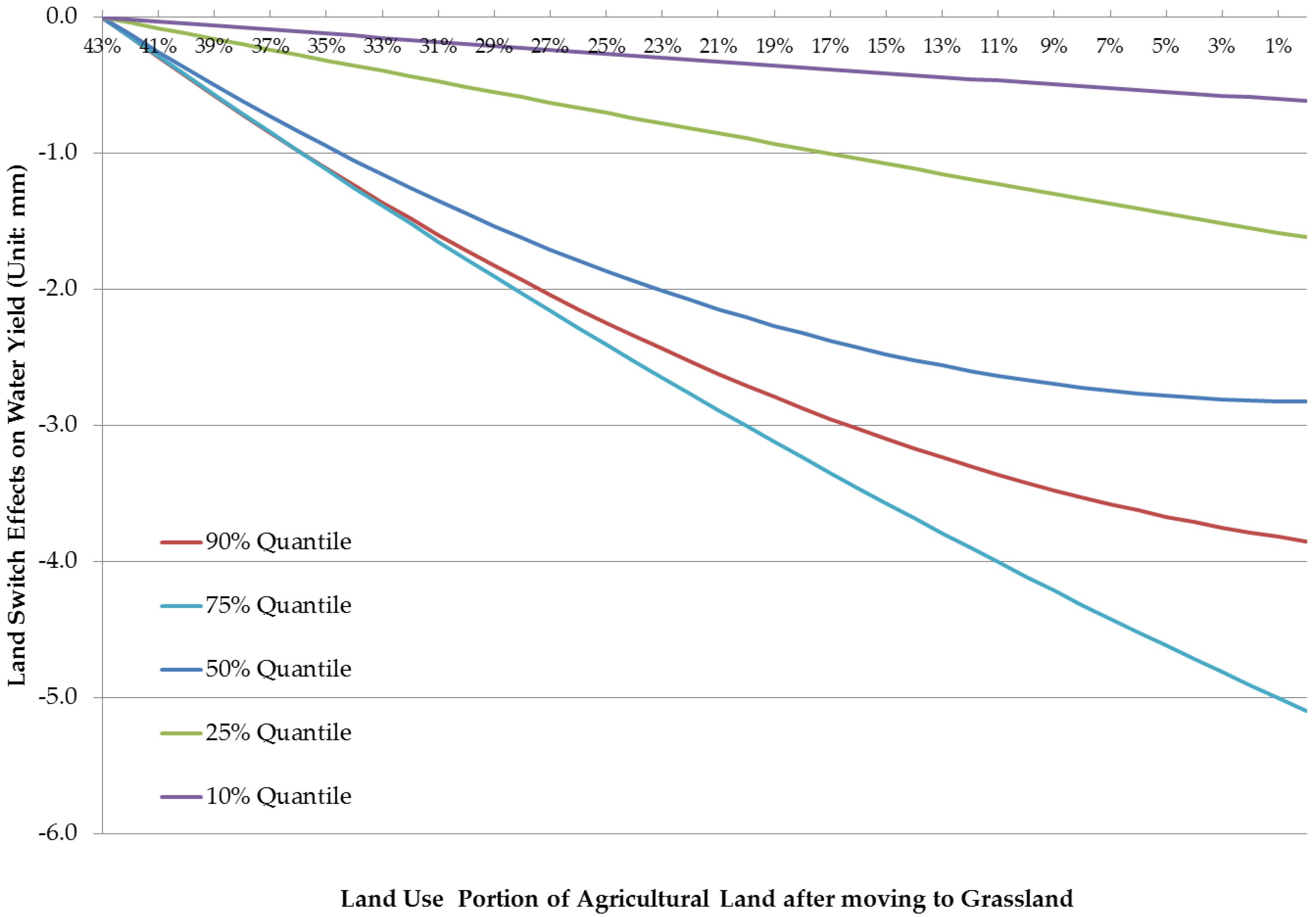
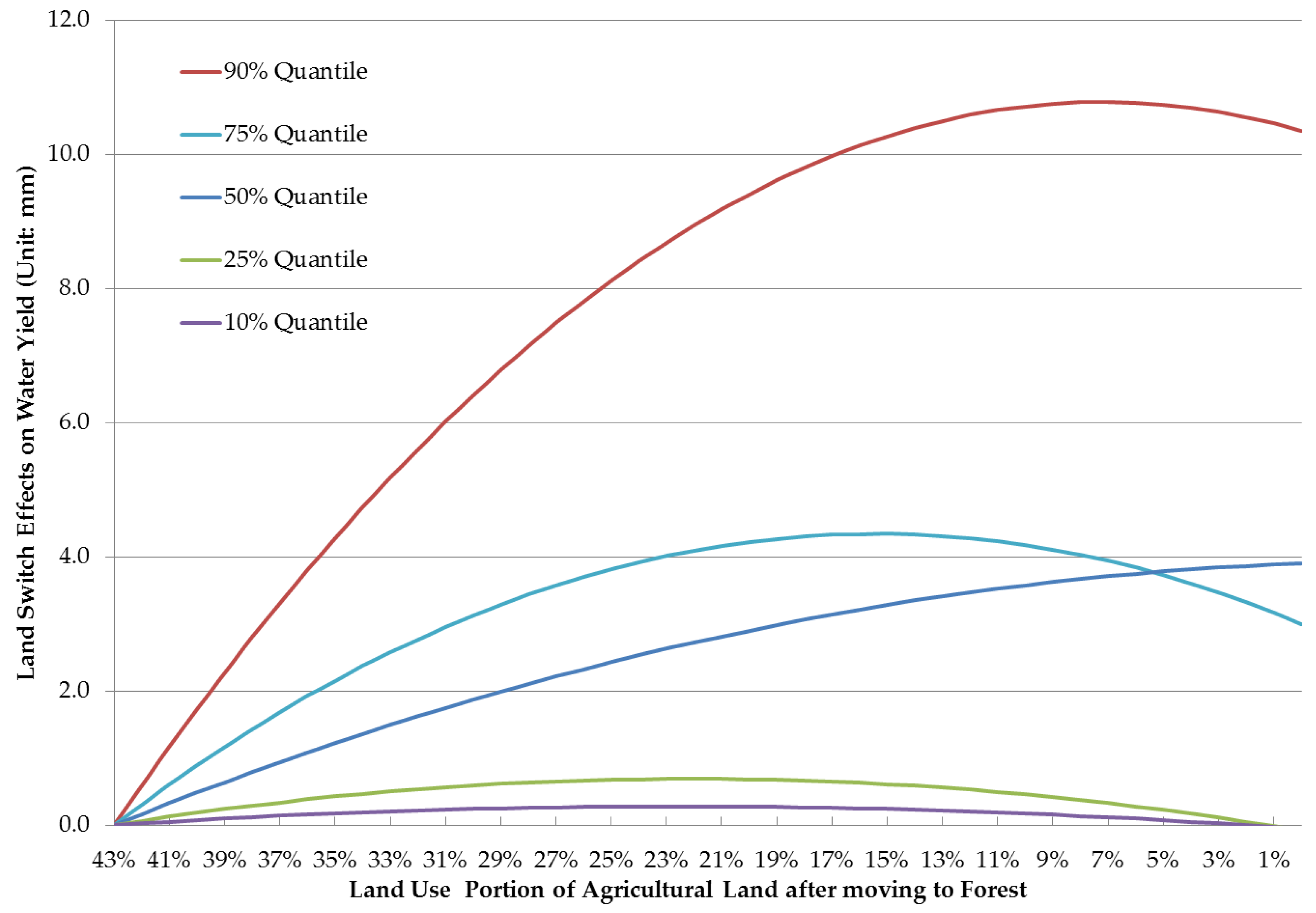
6. Analysis of Water Implications of Mitigation Strategy Choice
6.1. Effects under the Lower Carbon Price Scenarios
6.2. Effects under the Higher Carbon Price Scenarios
7. Conclusions
Author Contributions
Acknowledgments
Conflicts of Interest
Appendix A
References
- Pachauri, R.K.; Allen, M.R.; Barros, V.R.; Broome, J.; Cramer, W.; Christ, R.; Church, J.A.; Clarke, L.; Dahe, Q.; Dasgupta, P. Climate Change 2014: Synthesis Report. Contribution of Working Groups I, II to the Fifth Assessment Report of the Intergovernmental Panel on Climate Change; Cambridge University Press: Cambridge, UK; New York, NY, USA, 2014. [Google Scholar]
- McCarl, B.A.; Schneider, U.A. US agriculture’s role in a greenhouse gas emission mitigation world: An economic perspective. Rev. Agric. Econ. 2000, 22, 134–159. [Google Scholar] [CrossRef]
- Kindermann, G.; Obersteiner, M.; Sohngen, B.; Sathaye, J.; Andrasko, K.; Rametsteiner, E.; Schlamadinger, B.; Wunder, S.; Beach, R. Global cost estimates of reducing carbon emissions through avoided deforestation. Proc. Natl. Acad. Sci. USA 2008, 105, 10302–10307. [Google Scholar] [CrossRef] [PubMed]
- Smith, P.; Martino, D.; Cai, Z.; Gwary, D.; Janzen, H.; Kumar, P.; McCarl, B.A.; Ogle, S.M.; O’Mara, F.; Rice, C.; et al. Greenhouse Gas Mitigation in Agriculture. Philos. Trans. R. Soc. B Biol. Sci. 2008, 363, 789–813. [Google Scholar] [CrossRef] [PubMed]
- Golub, A.; Hertel, T.; Lee, H.L.; Rose, S.; Sohngen, B. The opportunity cost of land use and the global potential for greenhouse gas mitigation in agriculture and forestry. Resour. Energy Econ. 2009, 31, 299–319. [Google Scholar] [CrossRef]
- Smith, P.; Bustamante, M.; Ahammad, H.; Clark, H.; Dong, E.A.; Elsiddig, H.; Haberl, R.; Harper, J.; House, J.; Jafari, M.; et al. Agriculture, Forestry, Forestry and Other Land Use (AFOLU). In Climate Change 2014: Mitigation of Climate Change. Contribution of Working Group III to the Fifth Assessment Report of the Intergovernmental Panel on Climate Change; Cambridge University Press: Cambridge, UK; New York, NY, USA, 2014. [Google Scholar]
- Rose, S.K.; Ahammad, H.; Eickhout, B.; Fisher, B.; Kurosawa, A.; Rao, S.; Riahi, K.; van Vuuren, D.P. Land-based mitigation in climate stabilization. Energy Econ. 2012, 34, 365–380. [Google Scholar] [CrossRef]
- Bustamante, M.; Robledo-Abad, C.; Harper, R.; Mbow, C.; Ravindranat, N.H.; Sperling, F.; Haberl, H.; Siqueira Pinto, A.; Smith, P. Co-benefits, trade-offs, barriers and policies for greenhouse gas mitigation in the agriculture, forestry and other land use (AFOLU) sector. Glob. Chang. Biol. 2014, 20, 3270–3290. [Google Scholar] [CrossRef] [PubMed]
- IPCC. Climate Change 2007: Mitigation: Contribution of Working Group III to the Fourth Assessment Report of the Intergovernmental Panel on Climate Change; Metz, B., Davidson, O.R., Bosch, P.R., Dave, R., Meyer, L.A., Eds.; Cambridge University Press: Cambridge, UK; New York, NY, USA, 2007. [Google Scholar]
- Ruddiman, W.F. The anthropogenic greenhouse era began thousands of years ago. Clim. Chang. 2003, 61, 261–293. [Google Scholar] [CrossRef]
- Lal, R. Soil carbon sequestration impacts on global climate change and food security. Science 2004, 304, 1623–1627. [Google Scholar] [CrossRef] [PubMed]
- Murray, B.C.; Sohngen, B.; Sommer, A.; Depro, B.; Jones, K.; McCarl, B.A.; Gillig, D.; de Angelo, B.; Andrasko, K. Greenhouse Gas Mitigation Potential in US Forestry and Agriculture; Environmental Protection Agency, Office of Atmospheric Programs: Washington, DC, USA, 2005.
- McCarl, B.A. Bioenergy in a greenhouse mitigating world. Choices 2008, 23, 31–33. [Google Scholar]
- Baker, J.S.; Murray, B.C.; McCarl, B.A.; Feng, S.J.; Johansson, R. Implications of alternative agricultural productivity growth assumptions on land management, greenhouse gas emissions, and mitigation potential. Am. J. Agric. Econ. 2013, 95, 435–441. [Google Scholar] [CrossRef]
- Jackson, R.B.; Jobbágy, E.G.; Avissar, R.; Roy, S.B.; Barrett, D.; Cook, C.W.; Farley, K.A.; Le Maitre, D.C.; McCarl, B.A.; Murray, B.C. Trading water for carbon with biological carbon sequestration. Science 2005, 310, 1944–1947. [Google Scholar] [CrossRef] [PubMed]
- Elbakidze, L.; McCarl, B.A. Sequestration offsets versus direct emission reductions: Consideration of environmental co-effects. Ecol. Econ. 2007, 60, 564–571. [Google Scholar] [CrossRef]
- Gupta, S.C.; Kessler, A.C.; Brown, M.K.; Zvomuya, F. Climate and agricultural land use change impacts on streamflow in the upper midwestern United States. Water Resour. Res. 2015, 51, 5301–5317. [Google Scholar] [CrossRef]
- Mehdi, B.; Lehner, B.; Gombault, C.; Michaud, A.; Beaudin, I.; Sottile, M.F.; Blondlot, A. Simulated impacts of climate change and agricultural land use change on surface water quality with and without adaptation management strategies. Agric. Ecosyst. Environ. 2015, 213, 47–60. [Google Scholar] [CrossRef]
- Honisch, M.; Hellmeier, C.; Weiss, K. Response of surface and subsurface water quality to land use changes. Geoderma 2002, 105, 277–298. [Google Scholar] [CrossRef]
- Lal, R.; Delgado, J.A.; Groffman, P.M.; Millar, N.; Dell, C.; Rotz, A. Management to mitigate and adapt to climate change. J. Soil Water Conserv. 2011, 66, 276–285. [Google Scholar] [CrossRef]
- Mehdi, B.B. Scenarios and Implications of Land Use and Climate Change on Water Quality in Mesoscale Agricultural Watersheds. Ph.D. Thesis, McGill University, Montreal, QC, Canada, 2014. [Google Scholar]
- Holland, J.M. The environmental consequences of adopting conservation tillage in Europe: Reviewing the evidence. Agric. Ecosyst. Environ. 2004, 103, 1–25. [Google Scholar] [CrossRef]
- Yagi, K.; Tsuruta, H.; Kanda, K.; Minami, K. Effect of water management on methane emission from a Japanese rice paddy field: Automated methane monitoring. Glob. Biogeochem. Cycles 1996, 10, 255–267. [Google Scholar] [CrossRef]
- Sadras, V.O.; Grassini, P.; Steduto, P. Status of Water Use Efficiency of Main Crops. 2011. Available online: http://www.fao.org/fileadmin/templates/solaw/files/thematic_reports/TR_07_web.pdf (accessed on 16 September 2016).
- Carey, M.; Baraer, M.; Mark, B.G.; French, A.; Bury, J.; Young, K.R.; McKenzie, J.M. Toward hydro-social modeling: Merging human variables and the social sciences with climate-glacier runoff models (Santa River, Peru). J. Hydrol. 2014, 518, 60–70. [Google Scholar] [CrossRef]
- Perry, C. Efficient irrigation; inefficient communication; flawed recommendations. Irrig. Drain. 2007, 56, 367–378. [Google Scholar] [CrossRef]
- Pfeiffer, L.; Lin, C.C. Does efficient irrigation technology lead to reduced groundwater extraction? empirical evidence. J. Environ. Econ. Manag. 2014, 67, 189–208. [Google Scholar] [CrossRef]
- Raper, R.L. Subsoiling. In Encyclopedia of Soils in the Environment; Hillel, D., Ed.; Elsevier Ltd.: Oxford, UK, 2004; pp. 69–76. ISBN 9780123485304. [Google Scholar]
- Pikul, J.L.; Aase, J.K. Water infiltration and storage affected by subsoiling and subsequent tillage. Soil Sci. Soc. Am. J. 2003, 67, 859–866. [Google Scholar] [CrossRef]
- Wu, L.; Long, T.Y.; Liu, X.; Guo, J.S. Impacts of climate and land-use changes on the migration of non-point source nitrogen and phosphorus during rainfall-runoff in the Jialing River Watershed, China. J. Hydrol. 2012, 475, 26–41. [Google Scholar] [CrossRef]
- El-Khoury, A.; Seidou, O.; Lapen, D.R.; Que, Z.; Mohammadian, M.; Sunohara, M.; Bahram, D. Combined impacts of future climate and land use changes on discharge, nitrogen and phosphorus loads for a Canadian river basin. J. Environ. Manag. 2015, 151, 76–86. [Google Scholar] [CrossRef] [PubMed]
- Beasley, R.P. Erosion and sediment pollution control. In Erosion and Sediment Pollution Control; Iowa State University Press: Ames, Iowa, 1972; ISBN 19730707036. [Google Scholar]
- Moldenhauer, W.C.; Langdale, G.W.; Frye, W.; McCool, D.K.; Papendick, R.I.; Smika, D.E.; Fryrear, D.W. Conservation tillage for erosion control. J. Soil Water Conserv. 1983, 38, 144–151. [Google Scholar]
- Ongley, E.D. Control of Water Pollution from Agriculture; Food & Agriculture Organization of the United Nations: Rome, Italy, 1996. [Google Scholar]
- Bjorneberg, D.L.; Westermann, D.T.; Aase, J.K. Nutrient losses in surface irrigation runoff. J. Soil Water Conserv. 2002, 57, 524–529. [Google Scholar]
- Rabotyagov, S.; Campbell, T.; Jha, M.; Gassman, P.W.; Arnold, J.; Kurkalova, L.; Secchi, S.; Feng, H.; Kling, C.L. Least-cost control of agricultural nutrient contributions to the Gulf of Mexico hypoxic zone. Ecol. Appl. 2010, 20, 1542–1555. [Google Scholar] [CrossRef] [PubMed]
- Van Horn, H.H.; Wilkie, A.C.; Powers, W.J.; Nordstedt, R.A. Components of dairy manure management systems1. J. Dairy Sci. 1994, 77, 2008–2030. [Google Scholar] [CrossRef]
- Vergé, X.P.C.; Dyer, J.A.; Desjardins, R.L.; Worth, D. Greenhouse gas emissions from the Canadian pork industry. Livest. Sci. 2009, 121, 92–101. [Google Scholar] [CrossRef]
- Larsen, R.E.; Miner, J.R.; Buckhouse, J.C.; Moore, J.A. Water-quality benefits of having cattle manure deposited away from streams. Bioresour. Technol. 1994, 48, 113–118. [Google Scholar] [CrossRef]
- Kronvang, B.; Andersen, H.E.; Børgesen, C.; Dalgaard, T.; Larsen, S.E.; Bøgestrand, J.; Blicher-Mathiasen, G. Effects of policy measures implemented in Denmark on nitrogen pollution of the aquatic environment. Environ. Sci. Policy 2008, 11, 144–152. [Google Scholar] [CrossRef]
- Steinfeld, H.; Gerber, P.; Wassenaar, T.; Castel, V.; Rosales, M.; de Haan, C. Livestock’s Long Shadow. 2006. Available online: https://www.globalmethane.org/expo-docs/china07/postexpo/ag_gerber.pdf (accessed on 24 August 2017).
- Nabuurs, G.J.; Masera, O.; Andrasko, K.; Benitez-Ponce, P.; Boer, R.; Dutschke, M.; Elsiddig, E.; Ford-Robertson, J.; Abbott, P.C.; Karjalainen, T.; et al. Forestry. In Climate Change 2007: Mitigation. Contribution of Working Group III to the Fourth Assessment Report of the Intergovernmental Panel on Climate Change; Metz, B., Davidson, O.R., Bosch, P.R., Dave, R., Meyer, L.A., Eds.; Cambridge University Press: Cambridge, UK; New York, NY, USA, 2007. [Google Scholar]
- Wall, A. Effect of removal of logging residue on nutrient leaching and nutrient pools in the soil after clearcutting in a Norway spruce stand. For. Ecol. Manag. 2008, 256, 1372–1383. [Google Scholar] [CrossRef]
- Mattikalli, N.M.; Richards, K.S. Estimation of surface water quality changes in response to land use change: Application of the export coefficient model using remote sensing and geographical information system. J. Environ. Manag. 1996, 48, 263–282. [Google Scholar] [CrossRef]
- Fulton, S.; West, B. Forestry impacts on water quality. South. For. Resour. Assess. 2002, 21, 635. [Google Scholar]
- Lam, Q.D.; Schmalz, B.; Fohrer, N. The impact of agricultural Best Management Practices on water quality in a North German lowland catchment. Environ. Monit. Assess. 2011, 183, 351–379. [Google Scholar] [CrossRef] [PubMed]
- Calvin, K.; Edmonds, J.; Bond-Lamberty, B.; Clarke, L.; Kim, S.H.; Kyle, P.; Smith, S.J.; Thomson, A.; Wise, M. 2.6: Limiting climate change to 450 ppm CO2 equivalent in the 21st century. Energy Econ. 2009, 31, S107–S120. [Google Scholar] [CrossRef]
- Wise, M.; Calvin, K.; Thomson, A.; Clarke, L.; Bond-Lamberty, B.; Sands, R.; Smith, S.J.; Janetos, A.; Edmonds, J. Implications of limiting CO2 concentrations for land use and energy. Science 2009, 324, 1183–1186. [Google Scholar] [CrossRef] [PubMed]
- Grassi, G.; den Elzen, M.G.; Hof, A.F.; Pilli, R.; Federici, S. The role of the land use, land use change and forestry sector in achieving Annex I reduction pledges. Clim. Chang. 2012, 115, 873–881. [Google Scholar] [CrossRef]
- Van Vuuren, D.P.; Edmonds, J.; Kainuma, M.; Riahi, K.; Thomson, A.; Hibbard, K.; Hurtt, G.C.; Kram, T.; Krey, V.; Lamarque, J.F.; et al. The representative concentration pathways: An overview. Clim. Chang. 2011, 109, 5–31. [Google Scholar] [CrossRef]
- Leterme, B.; Mallants, D. Climate and land-use change impacts on groundwater recharge. In Proc. ModelCARE2011: Models-Repositories of Knowledge; IAHS Press: Wallingford, UK, 2011. [Google Scholar]
- Bhardwaj, A.K.; Zenone, T.; Jasrotia, P.; Robertson, G.P.; Chen, J.; Hamilton, S.K. Water and energy footprints of bioenergy crop production on marginal lands. GCB Bioenergy 2011, 3, 208–222. [Google Scholar] [CrossRef]
- Land Use & Water Quality. Available online: https://engineering.purdue.edu/SafeWater/watershed/landuse.html (accessed on 9 April 2018).
- Rhodes, A.L.; Newton, R.M.; Pufall, A. Influences of land use on water quality of a diverse New England watershed. Environ. Sci. Technol. 2001, 35, 3640–3645. [Google Scholar] [CrossRef] [PubMed]
- Wang, X. Integrating water-quality management and land-use planning in a watershed context. J. Environ. Manag. 2001, 61, 25–36. [Google Scholar] [CrossRef] [PubMed]
- Tong, S.T.; Chen, W. Modeling the relationship between land use and surface water quality. J. Environ. Manag. 2002, 66, 377–393. [Google Scholar] [CrossRef]
- DeFries, R.; Eshleman, K.N. Land-use change and hydrologic processes: A major focus for the future. Hydrol. Process. 2004, 18, 2183–2186. [Google Scholar] [CrossRef]
- Bahar, M.M.; Ohmori, H.; Yamamuro, M. Relationship between river water quality and land use in a small river basin running through the urbanizing area of Central Japan. Limnology 2008, 9, 19–26. [Google Scholar] [CrossRef]
- Lee, S.W.; Hwang, S.J.; Lee, S.B.; Hwang, H.S.; Sung, H.C. Landscape ecological approach to the relationships of land use patterns in watersheds to water quality characteristics. Lands. Urban Plan. 2009, 92, 80–89. [Google Scholar] [CrossRef]
- Binkley, D.; Brown, T.C. Forest practices as nonpoint sources of pollution in North America. J. Am. Water Resour. Assoc. 1993, 29, 729–740. [Google Scholar] [CrossRef]
- Weller, D.E.; Jordan, T.E.; Correll, D.L.; Liu, Z.J. Effects of land-use change on nutrient discharges from the Patuxent River watershed. Estuaries 2003, 26, 244–266. [Google Scholar] [CrossRef]
- Chappell, A.; Webb, N.P.; Butler, H.J.; Strong, C.L.; McTainsh, G.H.; Leys, J.F.; Viscarra Rossel, R.A. Soil organic carbon dust emission: An omitted global source of atmospheric CO2. Glob. Chang. Biol. 2013, 19, 3238–3244. [Google Scholar] [CrossRef] [PubMed]
- Robertson, G.P.; Bruulsema, T.W.; Gehl, R.J.; Kanter, D.; Mauzerall, D.L.; Rotz, C.A.; Williams, C.O. Nitrogen–climate interactions in US agriculture. Biogeochemistry 2013, 114, 41–70. [Google Scholar] [CrossRef]
- Van Dijk, P.M.; Kwaad, F.J.P.M.; Klapwijk, M. Retention of water and sediment by grass strips. Hydrol. Process. 1996, 10, 1069–1080. [Google Scholar] [CrossRef]
- Schnoor, J.L.; Doering, O.C.; Entekhabi, D.; Hiler, E.A.; Hullar, T.L.; Tilman, D.; Logan, W.; Huddleston, N. Water Implications of Biofuels Production in the United States; The National Academies Press: Washington, DC, USA, 2008. [Google Scholar]
- Smith, P.; Ashmore, M.R.; Black, H.I.; Burgess, P.J.; Evans, C.D.; Quine, T.A.; Thomson, A.M.; Hicks, K.; Orr, H.G. The role of ecosystems and their management in regulating climate, and soil, water and air quality. J. Appl. Ecol. 2013, 50, 812–829. [Google Scholar] [CrossRef]
- Pionke, H.B.; Urban, J.B. Effect of agricultural land use on ground-water quality in a small Pennsylvania watershed. Groundwater 1985, 23, 68–80. [Google Scholar] [CrossRef]
- Scanlon, B.R.; Jolly, I.; Sophocleous, M.; Zhang, L. Global impacts of conversions from natural to agricultural ecosystems on water resources: Quantity versus quality. Water Resour. Res. 2007, 43. [Google Scholar] [CrossRef]
- Pattanayak, S.K.; McCarl, B.A.; Sommer, A.; Murray, B.C.; Bondelid, T.; Gillig, D.; DeAngelo, B. Water quality co-effects of greenhouse gas mitigation in US agriculture. Clim. Chang. 2005, 71, 341–372. [Google Scholar] [CrossRef]
- Townsend, P.V.; Harper, R.J.; Brennan, P.D.; Dean, C.; Wu, S.; Smettem, K.R.J.; Cook, S.E. Multiple environmental services as an opportunity for watershed restoration. For. Policy Econ. 2012, 17, 45–58. [Google Scholar] [CrossRef]
- Iowa Department of Natural Resource. Iowa’s Water, Ambient Monitoring Program, Groundwater Availability Modeling. 2017. Available online: http://www.iowadnr.gov/Environmental-Protection/Water-Quality/Water-Monitoring/Groundwater (accessed on 16 September 2016).
- Gerbens-Leenes, W.; Hoekstra, A.Y.; van der Meer, T.H. The water footprint of bioenergy. Proc. Natl. Acad. Sci. USA 2009, 106, 10219–10223. [Google Scholar] [CrossRef] [PubMed]
- Arnold, J.G.; Srinivasan, R.; Muttiah, R.S.; Williams, J.R. Large area hydrologic modeling and assessment part I: model development. J. Am. Water Resour. Assoc. 1998, 34, 73–89. [Google Scholar] [CrossRef]
- Douglas-Mankin, K.R.; Srinivasan, R.; Arnold, J.G. Soil and Water Assessment Tool (SWAT) model: Current developments and applications. Trans. ASABE 2010, 53, 1423–1431. [Google Scholar] [CrossRef]
- Adams, D.M.; Alig, R.J.; McCarl, B.A.; Murray, B.C. FASOMGHG Conceptual Structure, and Specification: Documentation. 2005. Available online: http://agecon2.tamu.edu/people/faculty/mccarl-bruce/papers/1212FASOMGHG_doc.pdf (accessed on 9 May 2014).
- Beach, R.H.; Adams, D.M.; Alig, R.J.; Baker, J.S.; Latta, G.S.; McCarl, B.A.; Rose, S.K.; White, E. Model Documentation for the Forest and Agricultural Sector Optimization Model with Greenhouse Gases (FASOMGHG); RTI Project, (0210826.016); RTI International: Research Triangle Park, NC, USA, 2010. [Google Scholar]
- USDA 2012 Census of Agriculture. Available online: https://www.agcensus.usda.gov/Publications/2012/ (accessed on 20 October 2015).
- Arnold, J.G.; Moriasi, D.N.; Gassman, P.W.; Abbaspour, K.C.; White, M.J.; Srinivasan, R.; Santhi, C.; Harmel, R.D.; Van Griensven, A.; Van Liew, M.W.; et al. SWAT: Model use, calibration, and validation. Trans. ASABE 2012, 55, 1491–1508. [Google Scholar] [CrossRef]
- Daggupati, P.; Deb, D.; Srinivasan, R.; Yeganantham, D.; Mehta, V.M.; Rosenberg, N.J. Large-Scale Fine-Resolution Hydrological Modeling Using Parameter Regionalization in the Missouri River Basin. J. Am. Water Resour. Assoc. 2016, 52, 648–666. [Google Scholar] [CrossRef]
- Mehta, V.M.; Mendoza, K.; Daggupati, P.; Srinivasan, R.; Rosenberg, N.J.; Deb, D. High-resolution simulations of decadal climate variability impacts on water yield in the Missouri River basin with the Soil and Water Assessment Tool (SWAT). J. Hydrometeorol. 2016, 17, 2455–2476. [Google Scholar] [CrossRef]
- Cude, C.G. Oregon water quality index a tool for evaluating water quality management effectiveness. J. Am. Water Resour. Assoc. 2001, 37, 125–137. [Google Scholar] [CrossRef]
- Swamee, P.K.; Tyagi, A. Describing water quality with aggregate index. J. Environ. Eng. 2000, 126, 451–455. [Google Scholar] [CrossRef]
- NOAA Data Access. Available online: https://www.ncdc.noaa.gov/data-access (accessed on 8 March 2014).
- Japan Meteorological Agency, Tokyo Climate Center. Historical El Niño and La Niña Events. Available online: http://ds.data.jma.go.jp/tcc/tcc/products/elnino/ensoevents.html (accessed on 9 April 2018).
- Koenker, R. Quantile regression for longitudinal data. J. Multivar. Anal. 2004, 91, 74–89. [Google Scholar] [CrossRef]
- McCarl, B.A.; Spreen, T.H. Price endogenous mathematical programming as a tool for sector analysis. Am. J. Agric. Econ. 1980, 62, 87–102. [Google Scholar] [CrossRef]
- Alig, R.J.; Adams, D.M.; McCarl, B.A. Impacts of incorporating land exchanges between forestry and agriculture in sector models. J. Agric. Appl. Econ. 1998, 30, 389–401. [Google Scholar] [CrossRef]
- Lee, H.C. The Dynamic Role for Carbon Sequestration by the US Agricultural and Forest Sectors in Greenhouse Gas Emission Mitigation. Ph.D. Thesis, Texas A&M University, College Station, TX, USA, 2002. [Google Scholar]
- Lee, H.C.; McCarl, B.A.; Gillig, D. The dynamic competitiveness of US agricultural and forest carbon sequestration. Can. J. Agric. Econ. 2005, 53, 343–357. [Google Scholar] [CrossRef]
- Bache, S.H.M.; Dahl, C.M.; Kristensen, J.T. Headlights on tobacco road to low birthweight outcomes. Empir. Econ. 2013, 44, 1593–1633. [Google Scholar] [CrossRef]
- Molina-Navarro, E.; Trolle, D.; Martínez-Pérez, S.; Sastre-Merlín, A.; Jeppesen, E. Hydrological and water quality impact assessment of a Mediterranean limno-reservoir under climate change and land use management scenarios. J. Hydrol. 2014, 509, 354–366. [Google Scholar] [CrossRef]
- Zhang, H.; Huang, G.H.; Wang, D.; Zhang, X.; Li, G.; An, C.; Cui, Z.; Liao, R.; Nie, X. An integrated multi-level watershed-reservoir modeling system for examining hydrological and biogeochemical processes in small prairie watersheds. Water Res. 2012, 46, 1207–1224. [Google Scholar] [CrossRef] [PubMed]
- NOAA (National Oceanic and Atmospheric Administration) N.O.S. What are El Niño and La Niña? 2018. Available online: https://oceanservice.noaa.gov/facts/ninonina.html (accessed on 9 April 2018).
- Pieterse, N.M.; Bleuten, W.; Jørgensen, S.E. Contribution of point sources and diffuse sources to nitrogen and phosphorus loads in lowland river tributaries. J. Hydrol. 2003, 271, 213–225. [Google Scholar] [CrossRef]
- Ngoye, E.; Machiwa, J.F. The influence of land-use patterns in the Ruvu river watershed on water quality in the river system. Phys. Chem. Earth 2004, 29, 1161–1166. [Google Scholar] [CrossRef]
- Woli, K.P.; Nagumo, T.; Kuramochi, K.; Hatano, R. Evaluating river water quality through land use analysis and N budget approaches in livestock farming areas. Sci. Total Environ. 2004, 329, 61–74. [Google Scholar] [CrossRef] [PubMed]
- Sliva, L.; Williams, D.D. Buffer zone versus whole catchment approaches to studying land use impact on river water quality. Water Res. 2001, 35, 3462–3472. [Google Scholar] [CrossRef]
- Gunawardhana, W.D.T.M.; Jayawardhana, J.M.C.K.; Udayakumara, E.P.N. Impacts of agricultural practices on water quality in Uma Oya catchment area in Sri Lanka. Procedia Food Sci. 2016, 6, 339–343. [Google Scholar] [CrossRef]
- Miserendino, M.L.; Casaux, R.; Archangelsky, M.; Di Prinzio, C.Y.; Brand, C.; Kutschker, A.M. Assessing land-use effects on water quality, in-stream habitat, riparian ecosystems and biodiversity in Patagonian northwest streams. Sci. Total Environ. 2011, 409, 612–624. [Google Scholar] [CrossRef] [PubMed]
- Tu, J. Spatially varying relationships between land use and water quality across an urbanization gradient explored by geographically weighted regression. Appl. Geogr. 2011, 31, 376–392. [Google Scholar] [CrossRef]
- Seeboonruang, U. A statistical assessment of the impact of land uses on surface water quality indexes. J. Environ. Manag. 2012, 101, 134–142. [Google Scholar] [CrossRef] [PubMed]
- Ahearn, D.S.; Sheibley, R.W.; Dahlgren, R.A.; Anderson, M.; Johnson, J.; Tate, K.W. Land use and land cover influence on water quality in the last free-flowing river draining the western Sierra Nevada, California. J. Hydrol. 2005, 313, 234–247. [Google Scholar] [CrossRef]


| Variables | Mean | Std. Dev. | Max | Min |
|---|---|---|---|---|
| Water Quantity Per County Per Month | 7.179 | 15.559 | 304.259 | 0 |
| Water Quality Index 1 | 19.016 | 21.787 | 100 | 10 |
| Land Use (Proportion of Total Acres in a County) | ||||
| Urban | 0.038 | 0.056 | 0.702 | 6.30 × 10⁻¹⁰ |
| Cropped land | 0.426 | 0.325 | 0.962 | 0 |
| Acres for Continuous Crops | 0.129 | 0.119 | 0.547 | 0 |
| Irrigated Acres for Crops | 0.047 | 0.139 | 0.820 | 0 |
| Rotation Acres for Crops | 0.121 | 0.168 | 0.718 | 0 |
| Acres for Alfalfa and Hay | 0.129 | 0.167 | 0.640 | 0 |
| Grass Land | 0.282 | 0.311 | 0.986 | 1.35 × 10⁻⁹ |
| Wet lands | 0.012 | 0.019 | 0.171 | 1.23 × 10⁻¹⁰ |
| Forested lands | 0.079 | 0.128 | 0.755 | 4.07 × 10⁻¹⁰ |
| Climate Factors | ||||
| # of Days per year with Precipitation > 1.0 Inch (D_Precip) | 0.52 | 0.85 | 11 | 0 |
| # of Days per year with Minimum Temperature ≤ 32.0 ℉ (D_MinT) | 12.92 | 12.18 | 31 | 0 |
| # of Days per year with Maximum Temperature ≥ 90.0 ℉ (D_MaxT) | 2.47 | 4.94 | 30 | 0 |
| Total Precipitation in a Month (mm) (Total_Precip) | 54.15 | 51.76 | 1303.07 | 0 |
| Monthly Mean Temperature (℉) (M_MeanT) | 48.58 | 18.72 | 87.98 | −12.1 |
| El Niño Event Occurrence (Proportion of Years) (El Niño) | 0.24 | 0.43 | -- | -- |
| La Niña Event Occurrence (Proportion of Years) (La Niña) | 0.19 | 0.39 | -- | -- |
| Variables | Quantiles | ||||
|---|---|---|---|---|---|
| 10% | 25% | 50% | 75% | 90% | |
| Average Water Quantity Per County Per Month | 0.037 | 0.262 | 1.610 | 6.951 | 19.427 |
| Average Water Quality Per County Per Month 1 | 10 | 10 | 13.232 | 13.983 | 45.556 |
| Variables | Mean | Std. Dev. | Max | Min |
|---|---|---|---|---|
| Land Use (% of Total Acres) When WQI 1 = 10 | ||||
| Urban | 0.043 | 0.056 | 0.702 | 6.30 × 10⁻¹⁰ |
| Cropped land | 0.538 | 0.322 | 0.962 | 0 |
| Grass Land | 0.157 | 0.233 | 0.986 | 1.35 × 10⁻⁹ |
| Water | 0.012 | 0.017 | 0.171 | 1.23 × 10⁻¹⁰ |
| Forests | 0.076 | 0.120 | 0.755 | 4.07 × 10⁻¹⁰ |
| Land Use (% of Total Acres) When WQI 1 > 10 | ||||
| Urban | 0.034 | 0.056 | 0.702 | 6.30 × 10⁻¹⁰ |
| Cropped land | 0.318 | 0.288 | 0.962 | 0 |
| Grass Land | 0.402 | 0.329 | 0.986 | 1.35 × 10⁻⁹ |
| Water | 0.012 | 0.020 | 0.171 | 1.23 × 10⁻¹⁰ |
| Forests | 0.081 | 0.136 | 0.755 | 4.07 × 10⁻¹⁰ |
| Land Use (% of Total Acres) When WQI 1 > 13.232 | ||||
| Urban | 0.034 | 0.056 | 0.702 | 6.30 × 10⁻¹⁰ |
| Cropped land | 0.316 | 0.288 | 0.962 | 2.22 × 10⁻¹¹ |
| Grass Land | 0.403 | 0.329 | 0.986 | 1.35 × 10⁻⁹ |
| Water | 0.012 | 0.020 | 0.171 | 1.23 × 10⁻¹⁰ |
| Forests | 0.081 | 0.136 | 0.755 | 4.07 × 10⁻¹⁰ |
| Land Use (% of Total Acres) When WQI 1 > 13.983 | ||||
| Urban | 0.029 | 0.049 | 0.702 | 6.30 × 10⁻¹⁰ |
| Cropped land | 0.278 | 0.294 | 0.962 | 0 |
| Grass Land | 0.398 | 0.349 | 0.986 | 1.35 × 10⁻⁹ |
| Water | 0.012 | 0.021 | 0.171 | 1.23 × 10⁻¹⁰ |
| Forests | 0.070 | 0.132 | 0.755 | 4.07 × 10⁻¹⁰ |
| Land Use (% of Total Acres) When WQI > 45.556 | ||||
| Urban | 0.025 | 0.028 | 0.492 | 6.30 × 10⁻¹⁰ |
| Cropped land | 0.330 | 0.322 | 0.962 | 0 |
| Grass Land | 0.301 | 0.330 | 0.986 | 1.35 × 10⁻⁹ |
| Water | 0.019 | 0.025 | 0.171 | 1.23 × 10⁻¹⁰ |
| Forests | 0.040 | 0.109 | 0.755 | 4.07 × 10⁻¹⁰ |
| Variables | Quantile Regressions | OLS | ||||
|---|---|---|---|---|---|---|
| 10% | 25% | 50% | 75% | 90% | ||
| Land Use (% of Total Acres) | ||||||
| Urban | 3.452 | 6.882 | 9.126 | 8.149 | 7.300 | 0.819 |
| (0.790) *** | (1.635) *** | (3.477) *** | (5.014) | (8.915) | (1.714) | |
| Urban_squared | −4.144 | −8.074 | −10.227 | −8.273 | −4.763 | 12.875 |
| (1.770) ** | (3.123) *** | (6.155) * | (8.273) | (15.661) | (3.256) *** | |
| Cropped land | 3.373 | 8.029 | 17.143 | 26.331 | 21.200 | 21.329 |
| (0.392) *** | (0.768) *** | (1.459) *** | (3.925) *** | (5.194) *** | (0.565) *** | |
| Cropped land_squared | −3.222 | −8.146 | −17.746 | −26.825 | −19.022 | −18.018 |
| (0.353) *** | (0.748) *** | (1.503) *** | (4.104) *** | (5.974) *** | (0.587) *** | |
| Grass Land | −2.887 | −7.870 | −18.276 | −29.628 | −28.720 | −18.618 |
| (0.323) *** | (0.711) *** | (1.598) *** | (4.235) *** | (4.842) *** | (0.516) *** | |
| Grass Land_squared | 3.477 | 8.718 | 19.822 | 32.898 | 33.114 | 23.661 |
| (0.367) *** | (0.811) *** | (1.888) *** | (5.059) *** | (5.484) *** | (0.591) *** | |
| Forests | 3.862 | 8.861 | 18.578 | 39.557 | 75.484 | 45.161 |
| (0.457) *** | (1.073) *** | (2.640) *** | (5.266) *** | (8.359) *** | (0.739) *** | |
| Forests_squared | −3.416 | −7.679 | −12.091 | −30.176 | −65.077 | −38.965 |
| (1.279) *** | (3.175) ** | (7.874) | (12.321) ** | (16.528) *** | (1.389) *** | |
| Climate Factors | ||||||
| D_Precip | −0.384 | −0.823 | −0.601 | 0.204 | 0.440 | −4.405 |
| (0.120) *** | (0.158) *** | (0.172) *** | (0.251) | (0.449) | (0.117) *** | |
| D_Precip_squared | 0.374 | 0.723 | 0.550 | 0.225 | 0.157 | 2.366 |
| (0.114) *** | (0.150) *** | (0.155) *** | (0.166) | (0.206) | (0.031) *** | |
| D_MinT | 0.008 | 0.017 | 0.030 | 0.047 | 0.279 | 0.249 |
| (0.003) ** | (0.005) *** | (0.008) *** | (0.021) ** | (0.062) *** | (0.021) *** | |
| D_MinT_squared | −0.0001 | −0.0003 | −0.001 | −0.0005 | −0.005 | −0.002 |
| (0.0001) | (0.0001) ** | (0.0002) *** | (0.0005) | (0.002) *** | (0.001) *** | |
| D_MaxT | −0.011 | −0.018 | −0.036 | −0.094 | −0.214 | −0.461 |
| (0.004) ** | (0.007) ** | (0.014) *** | (0.026) *** | (0.054) *** | (0.030) *** | |
| D_MaxT_squared | −0.0001 | −0.0001 | 0.001 | 0.002 | 0.004 | 0.010 |
| (0.0002) | (0.0002) | (0.0004) | (0.001) *** | (0.001) *** | (0.001) *** | |
| Total_Precip | −0.0009 | −0.017 | −0.038 | −0.038 | 0.0003 | 0.127 |
| (0.004) | (0.004) *** | (0.004) *** | (0.005) *** | (0.010) | (0.002) *** | |
| Total_Precip_squared | 0.0001 | 0.0004 | 0.001 | 0.001 | 0.001 | 0.0002 |
| (0.00004) ** | (0.0001) *** | (0.0001) *** | (0.0001) *** | (0.0001) *** | (5.58 × 10⁻⁶) *** | |
| M_MeanT | 0.001 | −0.002 | −0.001 | −0.006 | 0.004 | −0.054 |
| (0.002) | (0.004) | (0.006) | (0.011) | (0.023) | (0.015) *** | |
| M_MeanT_squared | 0.0001 | 0.0001 | 0.0001 | 0.0002 | 0.001 | 0.002 |
| (0.00003) * | (0.0001) ** | (0.0001) | (0.0002) | (0.0003) ** | (0.0002) *** | |
| El Niño | −0.030 | −0.078 | −0.120 | −0.204 | −0.493 | −0.649 |
| (0.009) *** | (0.013) *** | (0.018) *** | (0.033) *** | (0.092) *** | (0.083) *** | |
| La Niña | 0.046 | 0.099 | 0.341 | 1.122 | 2.291 | 1.581 |
| (0.011) *** | (0.017) *** | (0.051) *** | (0.136) *** | (0.262) *** | (0.089) *** | |
| Variables | Quantile Regressions | OLS | ||||
|---|---|---|---|---|---|---|
| 10% | 25% | 50% | 75% | 90% | ||
| Water Quantity | - | 0.0002 | −0.0003 | −0.007 | 0.049 | 0.028 |
| - | (0.0002) | (0.001) | (0.004) * | (0.020) ** | (0.006) *** | |
| Land Use (% of Total Acres) | ||||||
| Urban | - | 0.023 | −1.550 | −2.718 | −26.323 | −7.146 |
| - | (0.984) | (2.418) | (7.527) | (30.513) | (3.126) ** | |
| Urban_squared | - | 0.190 | −0.889 | 0.906 | −51.018 | −18.631 |
| - | (1.741) | (5.381) | (5.561) | (50.042) | (5.937) *** | |
| Cropped land | - | −0.505 | −2.640 | 0.975 | −7.428 | −2.213 |
| - | (1.624) | (1.449) * | (7.831) | (26.117) | (1.037) ** | |
| Cropped land_squared | - | 0.516 | −0.408 | −4.835 | −38.580 | −9.760 |
| - | (1.596) | (0.662) | (1.677) *** | (26.104) | (1.075) *** | |
| Grass Land | - | −0.920 | 6.623 | −1.156 | −70.286 | −17.173 |
| - | (1.452) | (1.858) *** | (7.138) | (19.883) *** | (0.947) *** | |
| Grass Land_squared | - | 5.324 | −5.713 | 0.141 | 46.399 | 10.018 |
| - | (1.642) *** | (0.822) *** | (1.208) | (22.318) ** | (1.086) *** | |
| Forests | - | 0.541 | −3.552 | −5.407 | −142.099 | −59.158 |
| - | (1.608) | (1.687) ** | (8.623) | (30.269) *** | (1.373) *** | |
| Forests_squared | - | -0.698 | 4.928 | 8.116 | 175.860 | 79.821 |
| - | (2.073) | (2.994) * | (4.642) * | (59.798) *** | (2.543) *** | |
| Climate Factors | ||||||
| D_Precip | - | −0.001 | −0.047 | −0.203 | −0.056 | −1.407 |
| - | (0.004) | (0.023) ** | (0.061) *** | (0.925) | (0.215) *** | |
| D_Precip_squared | - | 0.001 | 0.019 | 0.034 | 0.022 | 0.528 |
| - | (0.002) | (0.007) *** | (0.017) ** | (0.207) | (0.058) *** | |
| D_MinT | - | −0.002 | −0.001 | 0.025 | −0.696 | −0.160 |
| - | (0.002) | (0.003) | (0.012) ** | (0.178) *** | (0.039) *** | |
| D_MinT_squared | - | −0.0001 | −0.0004 | −0.003 | −0.023 | −0.010 |
| - | (0.0001) | (0.0001) *** | (0.002) * | (0.005) *** | (0.001) *** | |
| D_MaxT | - | 0.001 | −0.004 | −0.080 | −0.171 | −0.320 |
| - | (0.002) | (0.005) | (0.027) *** | (0.184) | (0.055) *** | |
| D_MaxT_squared | - | −0.0001 | −0.0005 | −0.001 | −0.018 | −0.008 |
| - | (0.0001) | (0.0001) *** | (0.001) ** | (0.006) *** | (0.002) *** | |
| Total_Precip | - | −0.001 | −0.006 | −0.019 | −0.421 | −0.123 |
| - | (0.001) | (0.001) *** | (0.006) *** | (0.099) *** | (0.004) *** | |
| Total_Precip_squared | - | 0.0000 | 0.0001 | 0.00003 | 0.001 | 0.0001 |
| - | (0.0000) | (0.0000) *** | (0.00002) * | (0.0003) *** | (0.00001) *** | |
| M_MeanT | - | −0.007 | −0.033 | −0.272 | −3.891 | −1.455 |
| - | (0.007) | (0.009) *** | (0.162) * | (0.343) *** | (0.028) *** | |
| M_MeanT_squared | - | 0.0001 | 0.0003 | 0.003 | 0.031 | 0.014 |
| - | (0.0001) | (0.0001) *** | (0.001) ** | (0.003) *** | (0.0004) *** | |
| El Niño | - | −0.001 | −0.015 | −0.011 | 1.259 | 0.405 |
| - | (0.004) | (0.006) ** | (0.031) | (0.372) *** | (0.150) *** | |
| La Niña | - | −0.003 | −0.015 | −0.039 | 1.069 | 0.646 |
| - | (0.005) | (0.007) ** | (0.022) * | (0.363) *** | (0.163) *** | |
| Allowed Mitigation Policies in this Run | Land Use Proportion of | Effects on Water Quantity (mm) | Effects on Water Quality | ||
|---|---|---|---|---|---|
| Cropped land (%) | Grass Land (%) | Forests (%) | |||
| Baseline Scenario | 31.35 | 37.02 | 19.84 | - | - |
| Carbon Price of $5 at a 5% Increase Rate Per Year | |||||
| Afforestation | 31.47 | 36.97 | 19.67 | 0.0055 | −0.0045 |
| Crop Fertilization Reduction | 32.18 | 36.24 | 19.68 | 0.0767 | −0.0430 |
| Crop Tillage Shifts | 31.91 | 36.34 | 19.72 | 0.0616 | −0.0332 |
| Crop Management | 32.15 | 36.20 | 19.68 | 0.0738 | −0.0428 |
| Livestock Enteric and Manure | 31.61 | 36.86 | 19.69 | 0.0094 | −0.0101 |
| Bioenergy Use | 31.34 | 37.01 | 19.84 | −0.0027 | 0.0003 |
| Forest Management improvement | 32.81 | 37.72 | 17.29 | −0.2708 | 0.0144 |
| Simultaneous Use of All Strategies | 32.79 | 37.70 | 17.25 | −0.2745 | 0.0147 |
| Carbon Price of $10 at a 5% Increase Rate Per Year | |||||
| Afforestation | 31.93 | 36.72 | 19.81 | 0.0213 | −0.0212 |
| Crop Fertilization Reduction | 31.93 | 36.71 | 19.83 | 0.0244 | −0.0220 |
| Crop Tillage Shifts | 31.66 | 36.81 | 19.86 | 0.0099 | −0.0123 |
| Crop Management | 31.64 | 36.87 | 19.81 | 0.0008 | −0.0094 |
| Livestock Enteric and Manure | 31.93 | 36.72 | 19.75 | 0.0240 | −0.0217 |
| Bioenergy Use | 31.36 | 37.03 | 19.82 | 0.0010 | −0.0003 |
| Forest Management improvement | 32.88 | 37.81 | 17.49 | −0.2992 | 0.0182 |
| Simultaneous Use of All Strategies | 32.84 | 37.79 | 17.46 | −0.3053 | 0.0192 |
| Carbon Price of $30 at a 5% Increase Rate Per Year | |||||
| Afforestation | 27.65 | 46.38 | 17.63 | −0.7200 | 0.3180 |
| Crop Fertilization Reduction | 27.92 | 46.29 | 17.37 | −0.7386 | 0.3139 |
| Crop Tillage Shifts | 27.29 | 46.55 | 17.45 | −0.7722 | 0.3339 |
| Crop Management | 27.21 | 46.41 | 17.41 | −0.7843 | 0.3351 |
| Livestock Enteric and Manure | 27.50 | 46.38 | 17.40 | −0.7653 | 0.3268 |
| Bioenergy Use | 27.51 | 46.40 | 17.37 | −0.7683 | 0.3271 |
| Forest Management improvement | 29.75 | 46.07 | 15.03 | −0.9547 | 0.3041 |
| Simultaneous Use of All Strategies | 28.97 | 47.57 | 14.72 | −1.0494 | 0.3521 |
| Carbon Price of $50 at a 5% Increase Rate Per Year | |||||
| Afforestation | 29.02 | 44.50 | 18.16 | −0.5430 | 0.2425 |
| Crop Fertilization Reduction | 28.50 | 44.77 | 17.73 | −0.6423 | 0.2692 |
| Crop Tillage Shifts | 28.05 | 45.35 | 17.93 | −0.6482 | 0.2869 |
| Crop Management | 28.00 | 45.47 | 17.92 | −0.6530 | 0.2903 |
| Livestock Enteric and Manure | 28.38 | 45.22 | 17.58 | −0.6733 | 0.2819 |
| Bioenergy Use | 27.96 | 45.45 | 17.69 | −0.6888 | 0.2953 |
| Forest Management improvement | 30.82 | 42.03 | 16.00 | −0.7099 | 0.1893 |
| Simultaneous Use of All Strategies | 29.29 | 46.55 | 15.29 | −0.9462 | 0.3184 |
© 2018 by the authors. Licensee MDPI, Basel, Switzerland. This article is an open access article distributed under the terms and conditions of the Creative Commons Attribution (CC BY) license (http://creativecommons.org/licenses/by/4.0/).
Share and Cite
Yu, C.-H.; McCarl, B.A. The Water Implications of Greenhouse Gas Mitigation: Effects on Land Use, Land Use Change, and Forestry. Sustainability 2018, 10, 2367. https://doi.org/10.3390/su10072367
Yu C-H, McCarl BA. The Water Implications of Greenhouse Gas Mitigation: Effects on Land Use, Land Use Change, and Forestry. Sustainability. 2018; 10(7):2367. https://doi.org/10.3390/su10072367
Chicago/Turabian StyleYu, Chin-Hsien, and Bruce A. McCarl. 2018. "The Water Implications of Greenhouse Gas Mitigation: Effects on Land Use, Land Use Change, and Forestry" Sustainability 10, no. 7: 2367. https://doi.org/10.3390/su10072367
APA StyleYu, C.-H., & McCarl, B. A. (2018). The Water Implications of Greenhouse Gas Mitigation: Effects on Land Use, Land Use Change, and Forestry. Sustainability, 10(7), 2367. https://doi.org/10.3390/su10072367