Regional Differences in Energy and Environmental Performance: An Empirical Study of 283 Cities in China

Abstract
:1. Introduction
2. Methodology
2.1. Biennial Energy and Environmental Production Technology
- (1)
- Weak disposability assumption: If and , then . It means that we can not reduce undesirable outputs alone while keeping the desirable outputs constant. In practice, it is feasible to reduce the desirable outputs and undesirable outputs at the same time; undesirable outputs can be abated at the cost of a decrease in desirable output.
- (2)
- Null-jointness assumption: If and , then . Production must cease entirely in order to fully eliminate undesirable outputs.
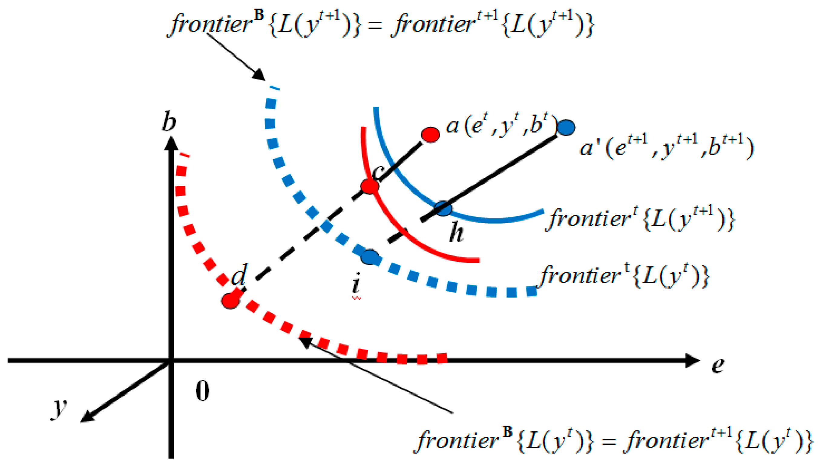
2.2. Biennial Luenberger Energy and Environmental Performance Index
2.3. Energy and Environmental Performance Measurement with Non-Radial DEA Model
2.4. Exploratory Spatial Data Analysis—Moran’s Index
2.5. Geographically Weighted Regression Model
3. Empirical Study
3.1. Data Source and Description
3.2. Results and Discussion
3.2.1. Static Energy and Environmental Performance
Descriptive Statistics of Energy and Environmental Performance
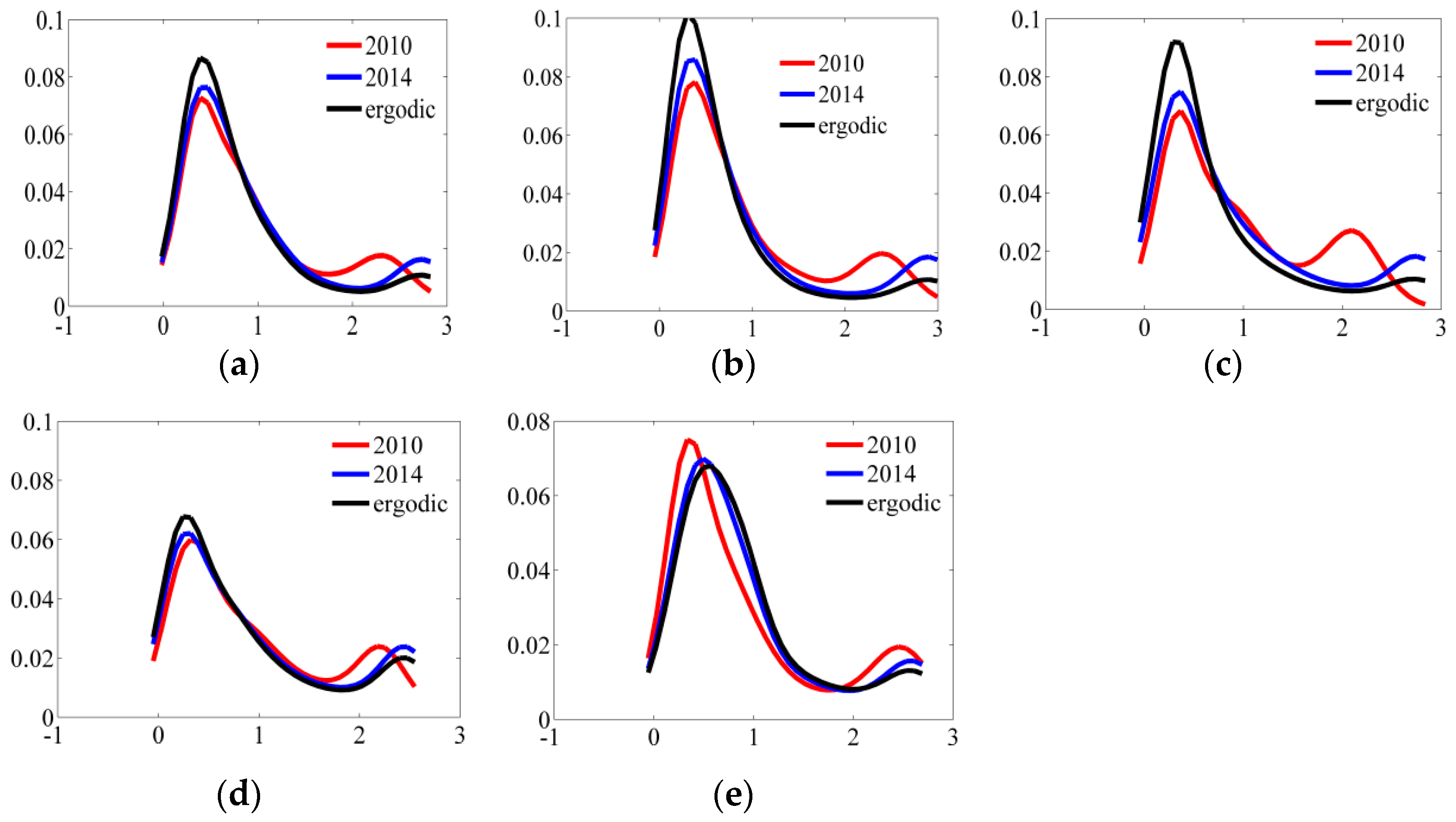
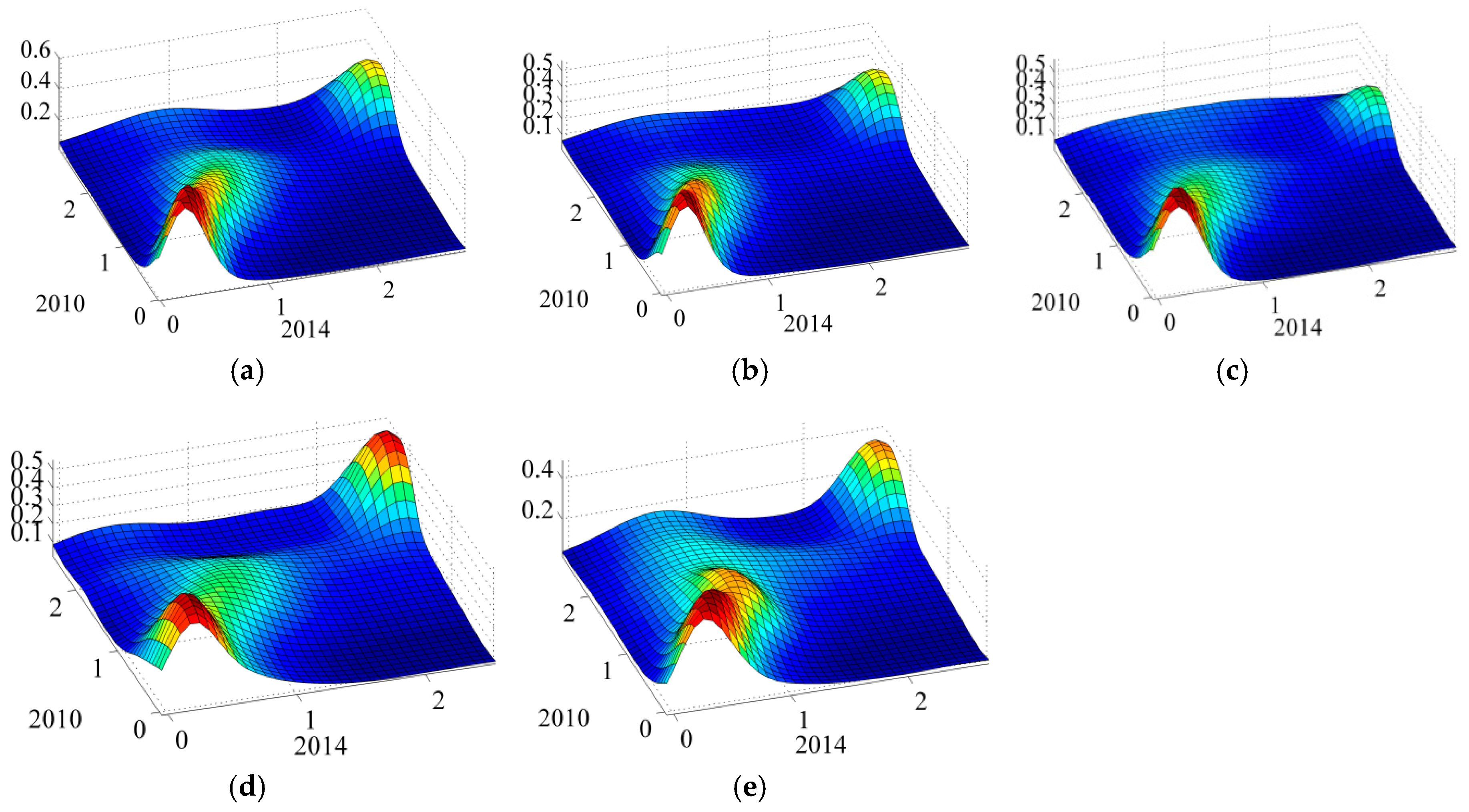
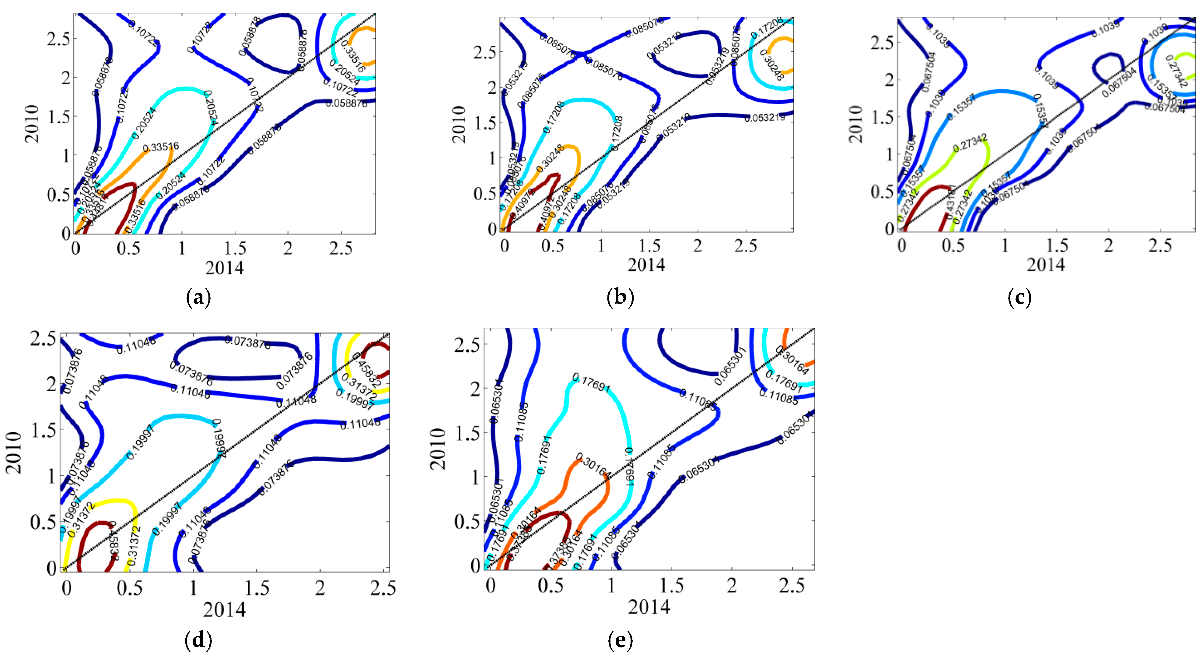
Distribution Dynamic Analysis of Energy and Environmental Performance
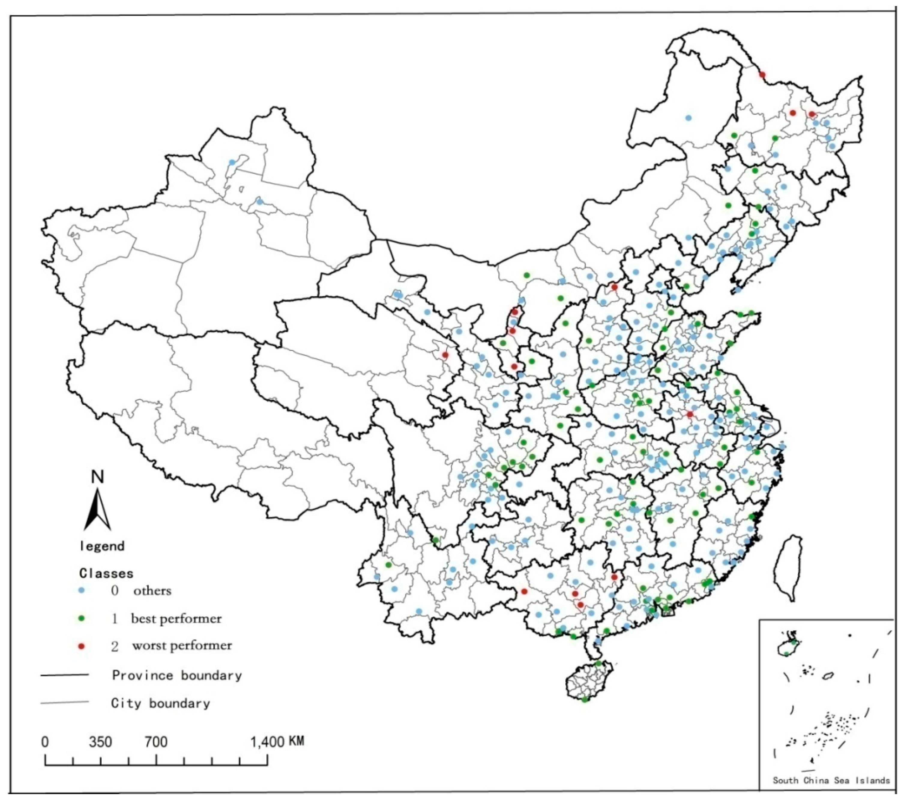
Analysis of Best and Worst Performers
3.2.2. Analysis of Dynamic Changes in Energy and Environmental Performance
National Level
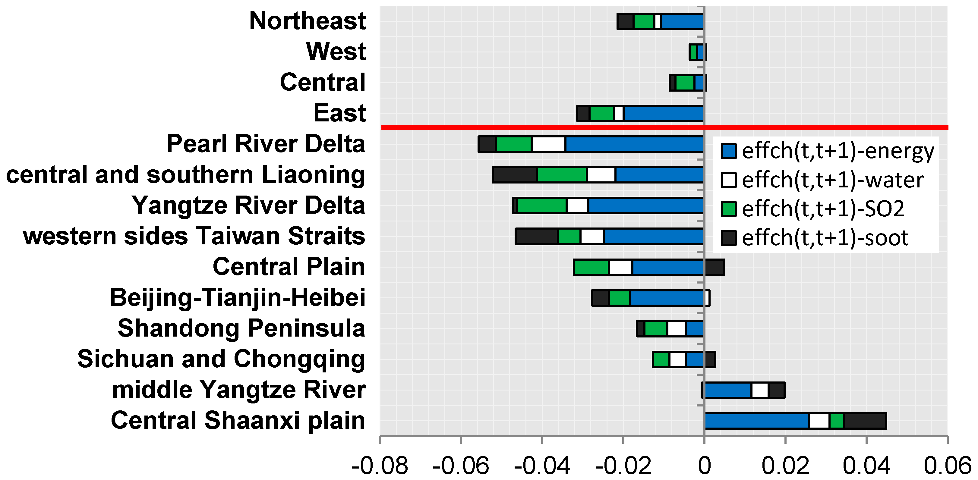
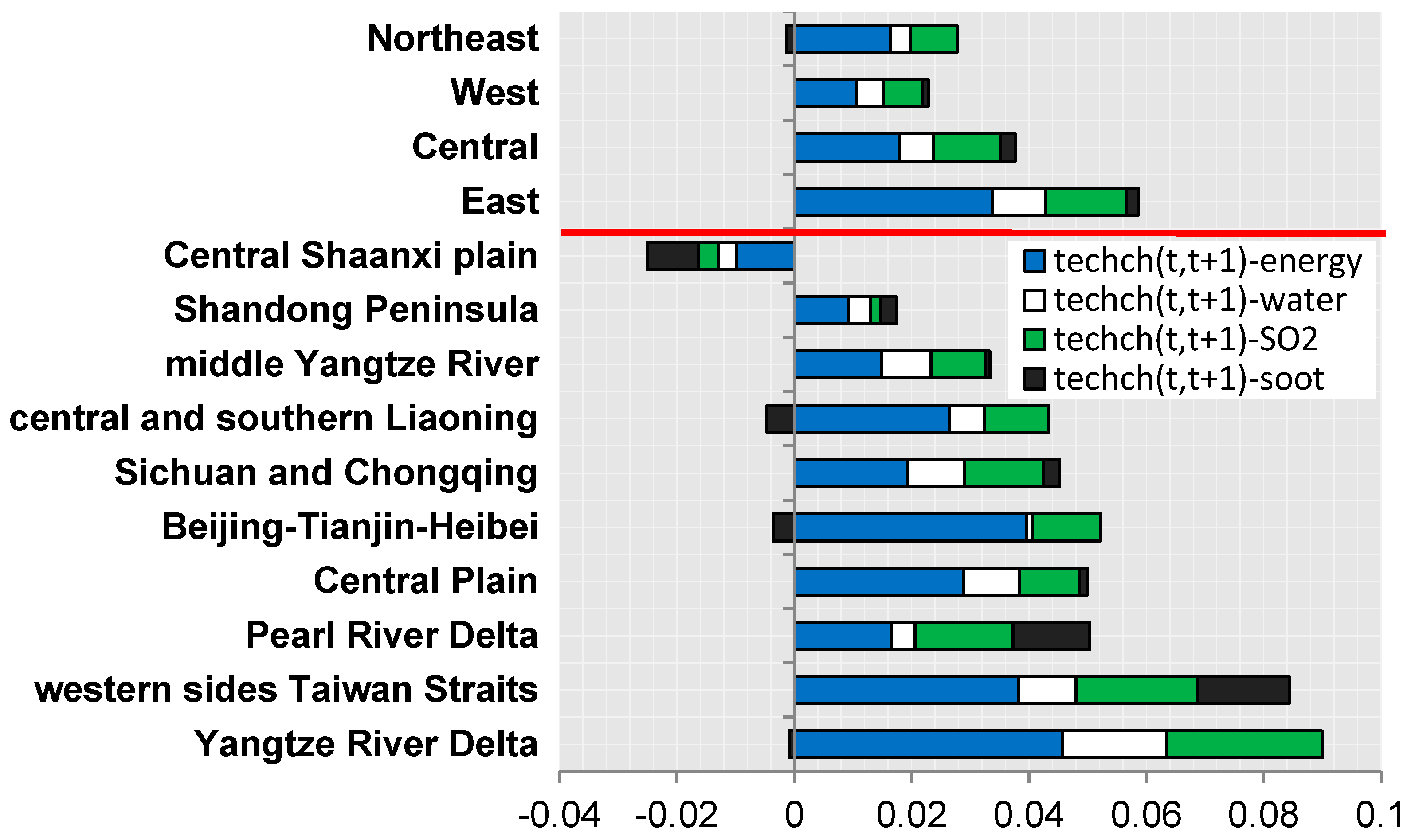
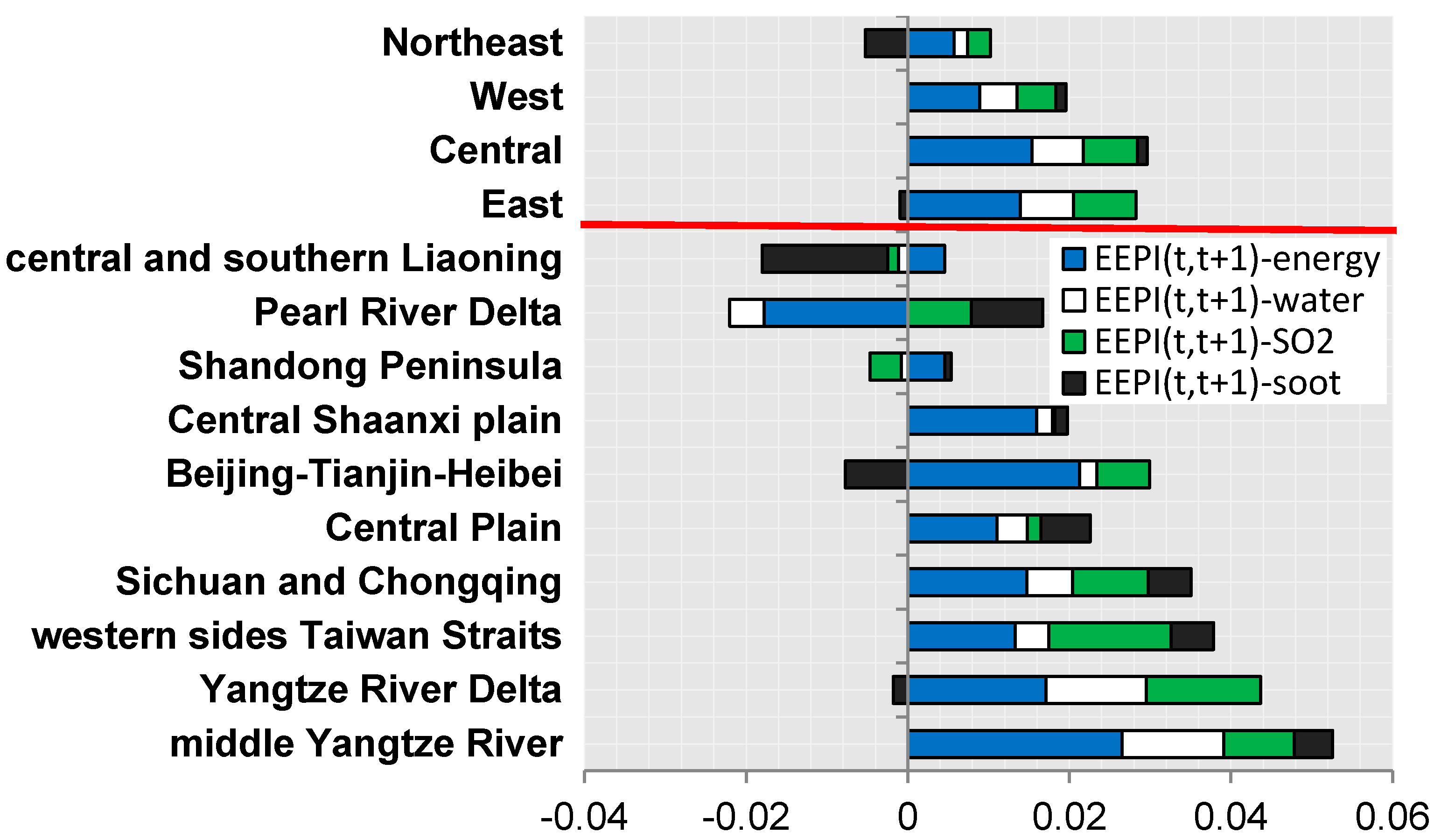
Regional Level
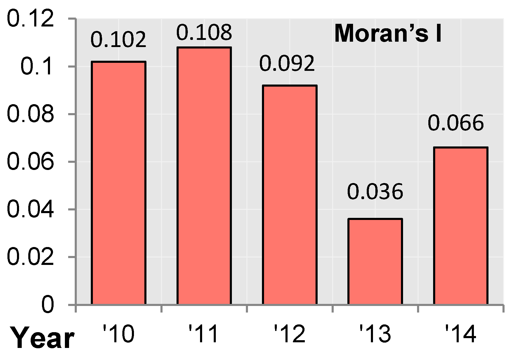
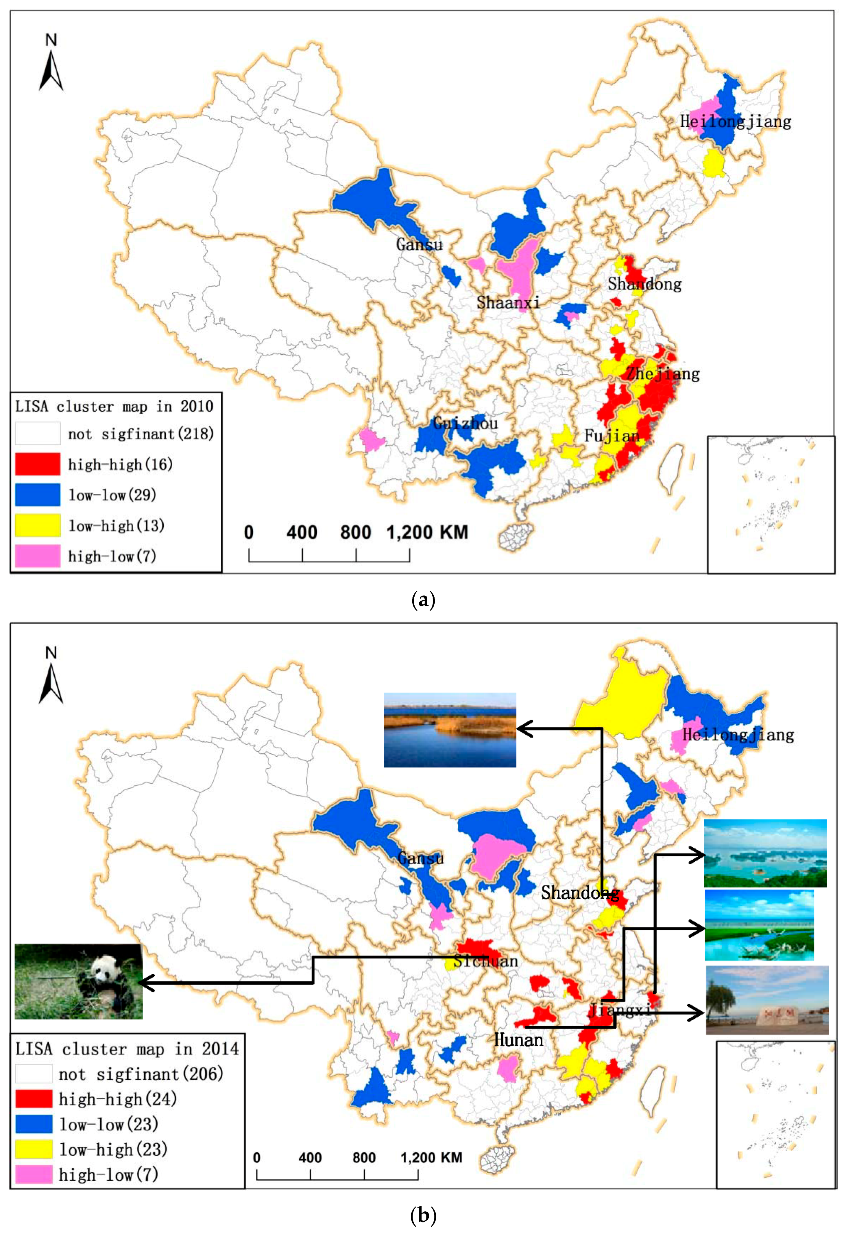
3.2.3. Analysis of Spatial Distribution Evolution on Energy and Environmental Performance Potential
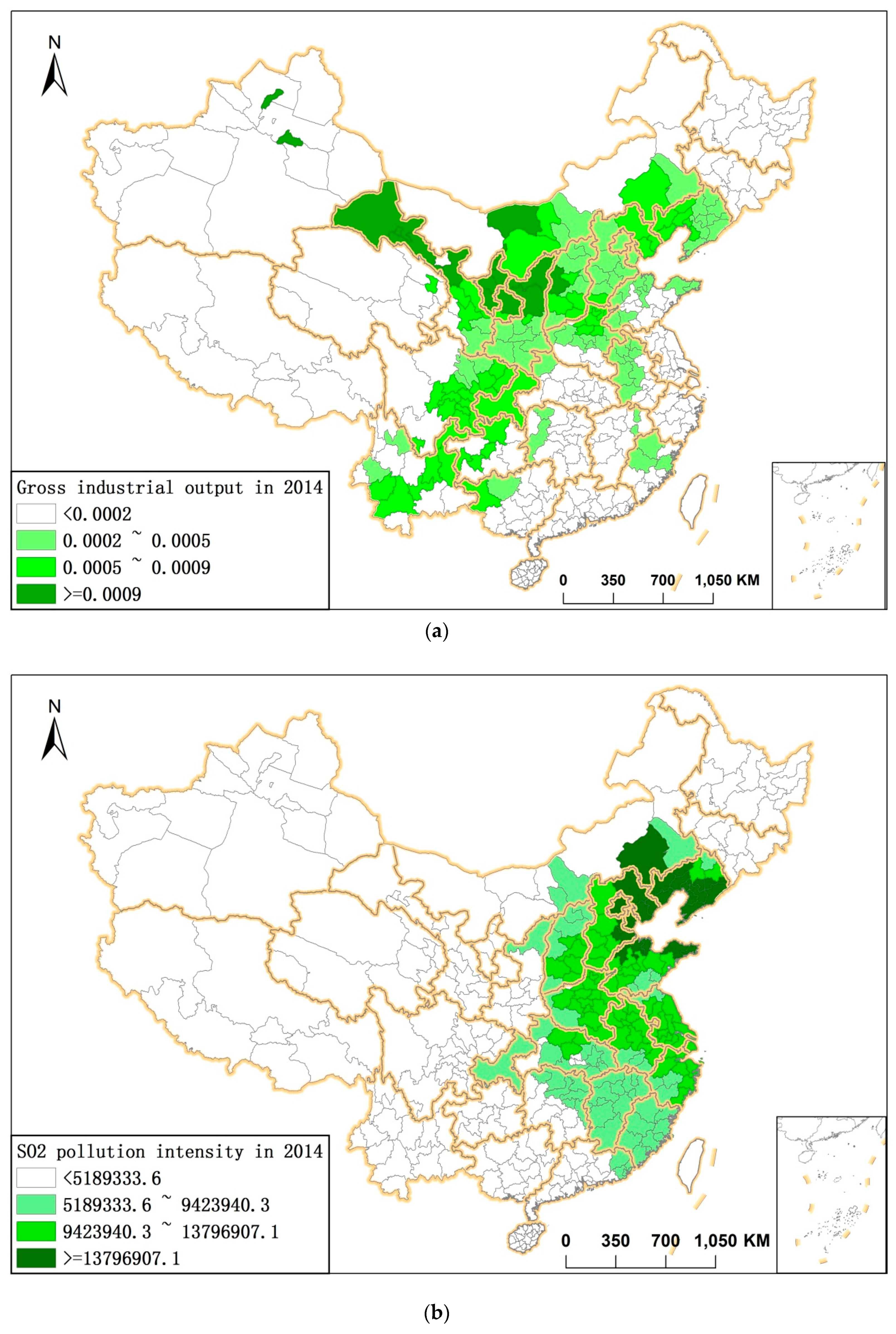
EEP Spatial Pattern
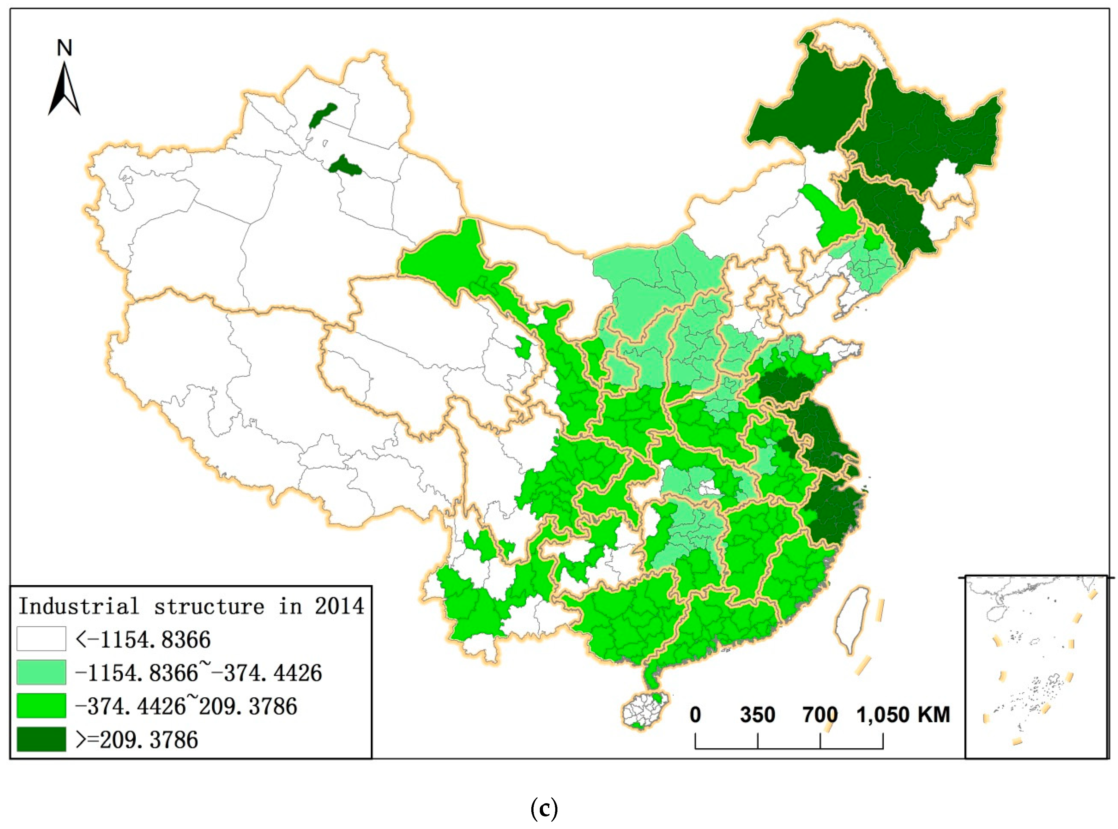
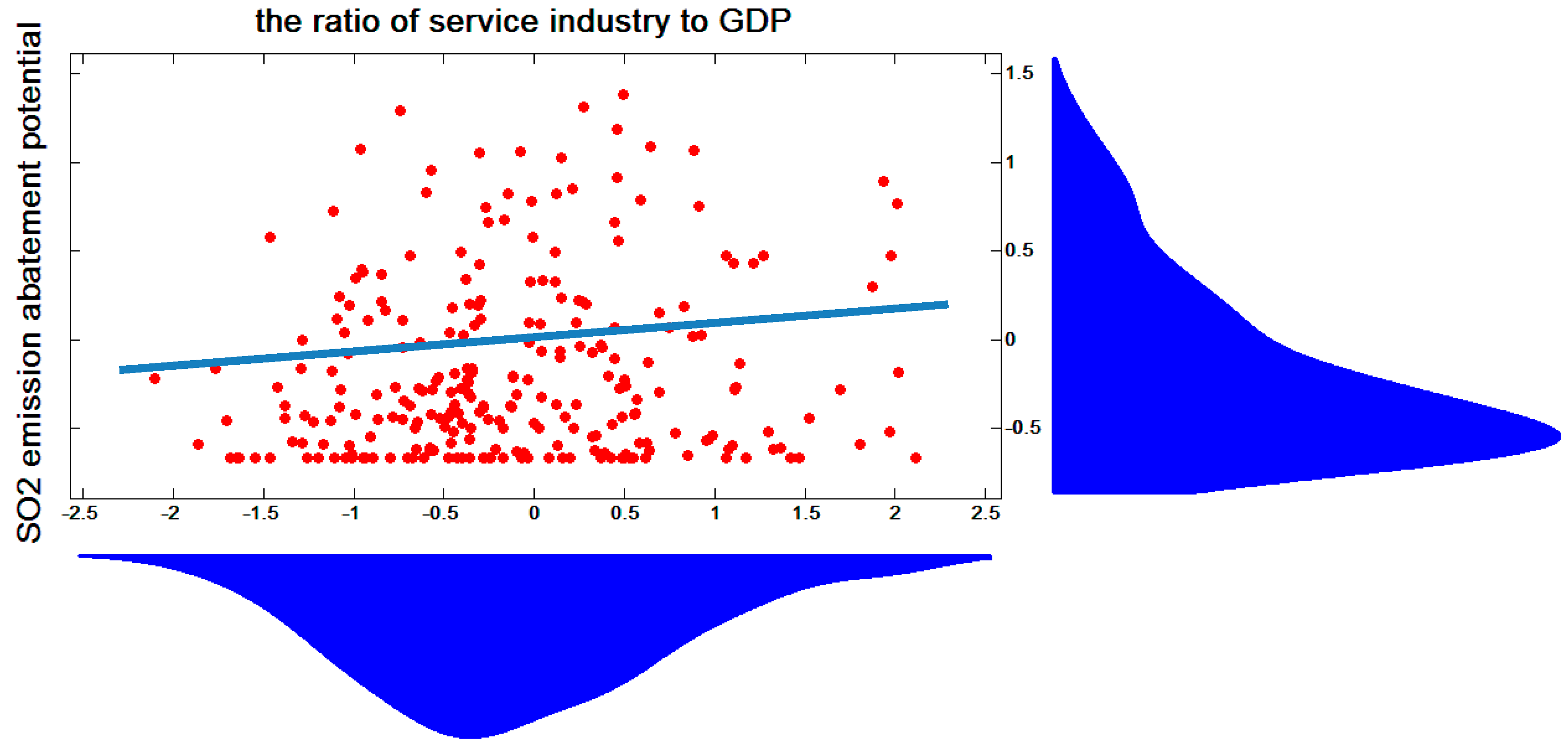
Influencing Factors on Energy and Environmental Performance Potential
4. Conclusions
Author Contributions
Funding
Acknowledgments
Conflicts of Interest
References
- Song, M.; Wang, S.; Yu, H.; Yang, L.; Wu, J. To reduce energy consumption and to maintain rapid economic growth: Analysis of the condition in China based on expended IPAT model. Renew. Sustain. Energy Rev. 2011, 15, 5129–5134. [Google Scholar] [CrossRef]
- British Peroleum Company. BP Statistical Review of World Energy 2017; British Peroleum Company: London, UK, 2017; Available online: https://www.bp.com/en/global/corporate/media/speeches/bp-statistical-review-of-world-energy-2017.html (accessed on 28 June 2017).
- Chen, J.; Song, M.; Xu, L. Evaluation of environmental efficiency in China using data envelopment analysis. Ecol. Indic. 2015, 52, 577–583. [Google Scholar] [CrossRef]
- Huang, R.-J.; Zhang, Y.; Bozzetti, C.; Ho, K.-F.; Cao, J.-J.; Han, Y.; Daellenbach, K.R.; Slowik, J.G.; Platt, S.M.; Canonaco, F. High secondary aerosol contribution to particulate pollution during haze events in China. Nature 2014, 514, 218–222. [Google Scholar] [CrossRef] [PubMed] [Green Version]
- Gao, J.; Woodward, A.; Vardoulakis, S.; Kovats, S.; Wilkinson, P.; Li, L.; Xu, L.; Li, J.; Yang, J.; Cao, L.; et al. Haze, public health and mitigation measures in China: A review of the current evidence for further policy response. Sci. Total Environ. 2017, 578, 148–157. [Google Scholar] [CrossRef] [PubMed] [Green Version]
- Ministry of Ecology and Environmental of the People’s Repuclic of China. Report on the State of China’s Environment in 2016; Ministry of Ecology and Environmental of the People’s Republic of China: Beijing, China, 2016. Available online: http://www.zhb.gov.cn/hjzl/zghjzkgb/lnzghjzkgb/ (accessed on 28 June 2018).
- Lepeule, J.; Schwartz, J. Chronic exposure to fine particles and mortality: An extended follow-up of the Harvard Six Cities study from 1974 to 2009. Environ. Health Perspect. 2012, 120, 965–970. [Google Scholar] [CrossRef] [PubMed] [Green Version]
- Lepeule, J.; Bind, M.A.; Baccarelli, A.A.; Koutrakis, P.; Tarantini, L.; Litonjua, A.; Sparrow, D.; Vokonas, P.; Schwartz, J.D. Epigenetic influences on associations between air pollutants and lung function in elderly men: The normative aging study. Environ. Health Perspect. 2014, 122, 566–572. [Google Scholar] [CrossRef] [PubMed] [Green Version]
- Farrell, M.J. The Measurement of Productive Efficiency. J. R. Stat. Soc. 1957, 120, 253–290. [Google Scholar] [CrossRef]
- Charnes, A.; Cooper, W.W.; Rhodes, E. Measuring the efficiency of decision-making units. Eur. J. Oper. Res. 1978, 2, 429–444. [Google Scholar] [CrossRef]
- Kuosmanen, T.; Kortelainen, M. Measuring Eco-efficiency of Production with Data Envelopment Analysis. J. Ind. Ecol. 2005, 9, 59–72. [Google Scholar] [CrossRef]
- Hu, J.L.; Wang, S.C. Total-factor energy efficiency of regions in China. Energy Policy 2006, 34, 3206–3217. [Google Scholar] [CrossRef]
- Song, M.; Yang, L.; Wu, J.; Lv, W. Energy saving in China: Analysis on the energy efficiency via bootstrap-DEA approach. Energy Policy 2013, 57, 1–6. [Google Scholar] [CrossRef]
- Özkara, Y.; Atak, M. Regional total-factor energy efficiency and electricity saving potential of manufacturing industry in Turkey. Energy 2015, 93, 495–510. [Google Scholar] [CrossRef]
- Feng, C.; Wang, M. Analysis of energy efficiency and energy savings potential in China’s provincial industrial sectors. J. Clean. Prod. 2017, 164, 1531–1541. [Google Scholar] [CrossRef]
- Zhou, D.Q.; Wu, F.; Zhou, X.; Zhou, P. Output-specific energy efficiency assessment: A data envelopment analysis approach. Appl. Energy 2016, 177, 117–126. [Google Scholar] [CrossRef]
- Honma, S.; Hu, J.L. Total-factor energy productivity growth of regions in Japan. Energy Policy 2009, 37, 3941–3950. [Google Scholar] [CrossRef]
- Wang, Q.W.; Zhou, D.Q. An empirical study on the change of total factor energy efficiency in China. Syst. Eng. 2008, 26, 74–80. (In Chinese) [Google Scholar]
- Chang, T.P.; Hu, J.L. Total-factor energy productivity growth, technical progress, and efficiency change: An empirical study of China. Appl. Energy 2010, 87, 3262–3270. [Google Scholar] [CrossRef]
- Zhang, X.P.; Cheng, X.M.; Yuan, J.H.; Gao, X.J. Total-factor energy efficiency in developing countries. Energy Policy 2011, 39, 644–650. [Google Scholar] [CrossRef]
- Färe, R.; Grosskopf, S.; Lovell, C.A.K.; Pasurka, C. Multilateral productivity comparisons when some outputs are undesirable: A nonparametric approach. Rev. Econ. Stat. 1989, 71, 90–98. [Google Scholar] [CrossRef]
- Kortelainen, M. Dynamic environmental performance analysis: A Malmquist index approach. Ecol. Econ. 2008, 64, 701–715. [Google Scholar] [CrossRef]
- Zhou, P.; Ang, B.W.; Poh, K.L. Measuring environmental performance under different environmental DEA technologies. Energy Econ. 2008, 30, 1–14. [Google Scholar] [CrossRef]
- Zhang, N.; Choi, Y. Total-factor carbon emission performance of fossil fuel power plants in China: A metafrontier non-radial Malmquist index analysis. Energy Econ. 2013, 40, 549–559. [Google Scholar] [CrossRef]
- Rashidi, K.; Saen, R.F. Measuring eco-efficiency based on green indicators and potentials in energy saving and undesirable output abatement. Energy Econ. 2015, 50, 18–26. [Google Scholar] [CrossRef]
- Sueyoshi, T.; Goto, M. Environmental assessment on coal-fired power plants in U.S. north-east region by DEA non-radial measurement. Energy Econ. 2015, 50, 125–139. [Google Scholar] [CrossRef]
- Xie, B.C.; Duan, N.; Wang, Y.S. Environmental efficiency and abatement cost of China’s industrial sectors based on a three-stage data envelopment analysis. J. Clean. Prod. 2016, 153, 626–636. [Google Scholar] [CrossRef]
- Molinos-Senante, M.; Maziotis, A.; Sala-Garrido, R. The Luenberger productivity indicator in the water industry: An empirical analysis for England and Wales. Util. Policy 2014, 30, 18–28. [Google Scholar] [CrossRef]
- Managi, S. Luenberger and Malmquist productivity indices in Japan, 1955–1995. Appl. Econ. Lett. 2003, 10, 581–584. [Google Scholar] [CrossRef]
- Mahlberg, B.; Sahoo, B.K. Radial and non-radial decompositions of Luenberger productivity indicator with an illustrative application. Int. J. Prod. Econ. 2011, 131, 721–726. [Google Scholar] [CrossRef]
- Azad, M.A.S.; Ancev, T. Measuring environmental efficiency of agricultural water use: A Luenberger environmental indicator. J. Environ. Manag. 2014, 145, 314–320. [Google Scholar] [CrossRef] [PubMed]
- Wang, K. Evaluation and decomposition of energy and environmental productivity change using DEA. In Handbook of Operations Analysis Using Data Envelopment Analysis; Hwang, S.N., Lee, H.S., Zhu, J., Eds.; Springer: Berlin, Germany, 2016; pp. 207–297. [Google Scholar]
- Wang, K.; Wei, Y.M. Sources of energy productivity change in China during 1997–2012: A decomposition analysis based on the Luenberger productivity indicator. Energy Econ. 2016, 54, 50–59. [Google Scholar] [CrossRef]
- Xian, Y.; Huang, Z. Sources of carbon productivity change: A decomposition and disaggregation analysis based on global Luenberger productivity indicator and endogenous directional distance function. Ecol. Indic. 2016, 66, 545–555. [Google Scholar]
- Wang, K.; Wei, Y.M.; Zhang, X. A comparative analysis of China’s regional energy and emission performance: Which is the better way to deal with undesirable outputs? Energy Policy 2012, 46, 574–584. [Google Scholar] [CrossRef]
- Zhou, P.; Wang, H. Energy and CO2 emission performance in electricity generation: A non-radial directional distance function approach. Eur. J. Oper. Res. 2012, 221, 625–635. [Google Scholar] [CrossRef]
- Zhou, P.; Poh, K.L.; Ang, B.W. A non-radial DEA approach to measuring environmental performance. Eur. J. Oper. Res. 2007, 178, 1–9. [Google Scholar] [CrossRef]
- Vlontzos, G.; Niavis, S.; Manos, B. A DEA approach for estimating the agricultural energy and environmental efficiency of EU countries. Renew. Sustain. Energy Rev. 2014, 40, 91–96. [Google Scholar] [CrossRef]
- Meng, F.; Su, B.; Thomson, E.; Zhou, D.; Zhou, P. Measuring China’s regional energy and carbon emission efficiency with DEA models: A survey. Appl. Energy 2016, 183, 1–21. [Google Scholar] [CrossRef]
- Geng, Z.Q.; Dong, J.G.; Han, Y.M.; Zhu, Q.X. Energy and environment efficiency analysis based on an improved environment DEA cross-model: Case study of complex chemical processes. Appl. Energy 2017, 205, 465–476. [Google Scholar] [CrossRef]
- Wang, J.; Zhao, T. Regional energy-environmental performance and investment strategy for China’s non-ferrous metals industry: A non-radial DEA based analysis. J. Clean. Prod. 2016, 163, 187–201. [Google Scholar] [CrossRef]
- Perez, K.; González-Araya, M.C.; Iriarte, A. Energy and GHG emission efficiency in the Chilean manufacturing industry: Sectoral and regional analysis by DEA and Malmquist indexes. Energy Econ. 2017, 66, 290–302. [Google Scholar] [CrossRef]
- Satterthwaite, D. Cities’ contribution to global warming: Notes on the allocation of greenhouse gas emissions. Environ. Urban. 2008, 20, 539–550. [Google Scholar] [CrossRef]
- Harris, P.G.; Chow, A.S.Y.; Symons, J. Greenhouse gas emissions from cities and regions: International implications revealed by Hong Kong. Energy Policy 2012, 44, 416–424. [Google Scholar] [CrossRef]
- Li, X.G.; Yang, J.; Liu, X.J. Analysis of Beijing’s environmental efficiency and related factors using a DEA model that considers undesirable outputs. Math. Comput. Model. 2013, 58, 956–960. [Google Scholar] [CrossRef]
- Yuan, P.; Cheng, S.; Sun, J.; Liang, W. Measuring the environmental efficiency of the Chinese industrial sector: A directional distance function approach. Math. Comput. Model. 2013, 58, 936–947. [Google Scholar] [CrossRef]
- Wang, Q.; Zhao, Z.; Shen, N.; Liu, T. Have Chinese cities achieved the win–win between environmental protection and economic development? From the perspective of environmental efficiency. Ecol. Indic. 2015, 51, 151–158. [Google Scholar] [CrossRef]
- Zhou, D.Q.; Wang, Q.; Su, B.; Zhou, P.; Yao, L.X. Industrial energy conservation and emission reduction performance in China: A city-level nonparametric analysis. Appl. Energy 2016, 166, 201–209. [Google Scholar] [CrossRef]
- Guo, J.; Zhu, D.; Wu, X.; Yan, Y. Study on Environment Performance Evaluation and Regional Differences of Strictly-Environmental-Monitored Cities in China. Sustainability 2017, 9, 2094. [Google Scholar] [CrossRef]
- Färe, R.; Grosskopf, S. Directional distance functions and slacks-based measures of efficiency. Eur. J. Oper. Res. 2010, 200, 320–322. [Google Scholar] [CrossRef]
- Pastor, J.T.; Asmild, M.; Lovell, C.A.K. The biennial Malmquist productivity change index. Soc. Econ. Plan. Sci. 2011, 45, 10–15. [Google Scholar] [CrossRef]
- Jenks, G.F. The Data Model Concept in Statistical Mapping. Int. Yearb. Cartogr. 1967, 7, 186–190. [Google Scholar]
- Picazotadeo, A.J.; Castillo, J.; Beltránesteve, M. A Dynamic Approach to Measuring Ecological-Economic Performance with Directional Distance Functions: Greenhouse Gas Emissions in the European Union; Working Papers1304; Department of Applied Economics II, Universidad de Valencia: València, Spain, 2013. [Google Scholar]
- Chambers, R.G.; Chung, Y.; Färe, R. Benefit and distance functions. J. Econ. Theory 1995, 70, 407–419. [Google Scholar] [CrossRef]
- Wang, H.; Zhou, P.; Zhou, D.Q. Scenario-based energy efficiency and productivity in China: A non-radial directional distance function analysis. Energy Econ. 2013, 40, 795–803. [Google Scholar] [CrossRef]
- Getis, A.; Ord, J.K. The analysis of spatial association by use of distance statistics. Geogra. Anal. 1992, 24, 189–206. [Google Scholar] [CrossRef]
- Brunsdon, C.; Fotheringham, A.S.; Charlton, M.E. Geographically weighted regression: A method for exploring spatial nonstationarity. Geogr. Anal. 1996, 28, 281–298. [Google Scholar] [CrossRef]
- Fotheringham, A.S.; Brunsdon, C.; Charlton, M. Geographically weighted regression: The analysis of spatially varying relationships. Am. J. Agric. Econ. 2004, 86, 554–556. [Google Scholar]
- Brunsdon, C.; Fotheringham, A.S.; Charlton, M. Geographically weighted summary statistics—A framework for localised exploratory data analysis. Comput. Environ. Urban Syst. 2002, 26, 501–524. [Google Scholar] [CrossRef]
- National Bureau of Statistics of the People’s Republic of China. The China City Statistical Yearbook 2011–2015; National Bureau of Statistics of the People’s Republic of China: Beijing, China, 2011–2015.
- National Bureau of Statistics of the People’s Republic of China. The China Provincial Statistical Yearbook 2011–2015; National Bureau of Statistics of the People’s Republic of China: Beijing, China, 2011–2015. Available online: http://www.stats.gov.cn/tjsj/ndsj/ (accessed on 28 June 2018).
- Quah, D. Empirical cross-section dynamics in economic growth. Eur. Econ. Rev. 1992, 37, 426–434. [Google Scholar] [CrossRef]
- Quah, D. Empirics for economic growth and convergence. Eur. Econ. Rev. 1996, 40, 1353–1375. [Google Scholar] [CrossRef] [Green Version]
- Quah, D.T. Empirics for growth and distribution: Stratification, polarization, and convergence clubs. J. Econ. Growth 1997, 2, 27–59. [Google Scholar] [CrossRef]
- Meng, F.Y.; Fan, L.W.; Zhou, P.; Zhou, D.Q. Measuring environmental performance in China’s industrial sectors with non-radial DEA. Math. Comput. Model. 2013, 58, 1047–1056. [Google Scholar] [CrossRef]
- Deng, L.J.; Zhang, P.Y.; Ping, L.I. Equilibrium of population and economic development in the top ten urban agglomerations in China. J. Grad. Sch. Chin. Acad. Sci. 2010, 27, 154–162. (In Chinese) [Google Scholar]
- Zeng, P.; Chen, F. Empirical research of “energy-environment-economy” comprehensive accounting system of the top ten urban agglomerations in china. Forum Sci. Technol. China 2012, 29, 62–66. (In Chinese) [Google Scholar]
- Peng, L.; Zhang, Y.; Wang, Y.; Zeng, X.; Peng, N.; Yu, A. Energy efficiency and influencing factor analysis in the overall Chinese textile industry. Energy 2015, 93, 1222–1229. [Google Scholar] [CrossRef] [Green Version]
- Fan, Y.; Bai, B.; Qi, Q.; Peng, K.; Yue, Z.; Jing, G. Study on eco-efficiency of industrial parks in China based on data envelopment analysis. J. Environ. Manag. 2017, 192, 107–115. [Google Scholar] [CrossRef] [PubMed]
- Su, B.; Zhan, M.; Zhai, J.; Wang, Y.; Fischer, T. Spatio-temporal variation of haze days and atmospheric circulation pattern in China (1961–2013). Quat. Int. 2015, 380, 14–21. [Google Scholar] [CrossRef]
- Zhang, J.; Chen, J.; Xia, X.; Che, H.; Fan, X.; Xie, Y.; Han, Z.; Chen, H.; Lu, D. Heavy aerosol loading over the Bohai Bay as revealed by ground and satellite remote sensing. Atmos. Environ. 2015, 124, 252–261. [Google Scholar] [CrossRef]
- Zhou, M.; Zhang, Y.; Han, Y.; Wu, J.; Du, X.; Xu, H.; Feng, Y.; Han, S. Spatial and temporal characteristics of PM2.5 acidity during autumn in marine and coastal area of Bohai Sea, China, based on two-site contrast. Atmos. Res. 2018, 202, 196–204. [Google Scholar] [CrossRef]
- He, C.; Huang, Z.; Ye, X. Spatial heterogeneity of economic development and industrial pollution in urban China. Stoch. Environ. Res. Risk Assess. 2014, 28, 767–781. [Google Scholar] [CrossRef]
- Hu, Z.; Miao, J.; Miao, C. Agglomeration characteristics of industrial pollution and their influencing factors on the scale of cities in China. Dili Yanjiu (Geogr. Res.) 2016, 35, 1470–1482. (In Chinese) [Google Scholar]


| Index | Variable | Unit | Quantity | Mean | St.Dev | Min | Max |
|---|---|---|---|---|---|---|---|
| Non-energy input | Labor force | 10 thousand persons | 283 × 5 | 19.16 | 28.18 | 0.39 | 260.92 |
| Current assets | billion Yuan | 283 × 5 | 116.27 | 196.44 | 0. 83 | 1808.43 | |
| Fixed assets | billion Yuan | 283 × 5 | 90.15 | 106.34 | 0.86 | 827.94 | |
| Energy input | Industrial electricity | 100 million kWh | 283 × 5 | 60.19 | 91.97 | 0.045 | 805.76 |
| Desirable output | Gross industrial output | billion Yuan | 283 × 5 | 310.31 | 423.71 | 1.53 | 3278.23 |
| Undesirable output | Industrial wastewater | million tons | 283 × 5 | 74.71 | 84.99 | 0.23 | 868.04 |
| Industrial sulfur dioxide | thousand tons | 283 × 5 | 58.78 | 57.33 | 0.002 | 572.75 | |
| Industrial soot | thousand tons | 283 × 5 | 41.71 | 188.64 | 0.034 | 5168.81 |
| Performance (Efficiency) | Area | Quantity | Mean | St.Dev | Min | Max |
|---|---|---|---|---|---|---|
| Total | East | 87 × 5 | 0.473 | 0.298 | 0.069 | 1.000 |
| China | 283 × 5 | 0.365 | 0.292 | 0.016 | 1.000 | |
| Central | 99 × 5 | 0.362 | 0.282 | 0.031 | 1.000 | |
| Northeast | 33 × 5 | 0.272 | 0.236 | 0.025 | 1.000 | |
| West | 64 × 5 | 0.270 | 0.276 | 0.016 | 1.000 | |
| Energy | East | 87 × 5 | 0.456 | 0.328 | 0.042 | 1.000 |
| Central | 99 × 5 | 0.364 | 0.304 | 0.012 | 1.000 | |
| China | 283 × 5 | 0.358 | 0.315 | 0.008 | 1.000 | |
| West | 64 × 5 | 0.259 | 0.291 | 0.008 | 1.000 | |
| Northeast | 33 × 5 | 0.257 | 0.253 | 0.019 | 1.000 | |
| Wastewater | East | 87 × 5 | 0.418 | 0.326 | 0.015 | 1.000 |
| China | 283 × 5 | 0.355 | 0.308 | 0.011 | 1.000 | |
| Central | 99 × 5 | 0.347 | 0.303 | 0.038 | 1.000 | |
| Northeast | 33 × 5 | 0.333 | 0.283 | 0.024 | 1.000 | |
| West | 64 × 5 | 0.280 | 0.292 | 0.011 | 1.000 | |
| SO2 | East | 87 × 5 | 0.481 | 0.330 | 0.037 | 1.000 |
| China | 283 × 5 | 0.358 | 0.321 | 0.007 | 1.000 | |
| Central | 99 × 5 | 0.338 | 0.314 | 0.020 | 1.000 | |
| Northeast | 33 × 5 | 0.281 | 0.266 | 0.017 | 1.000 | |
| West | 64 × 5 | 0.264 | 0.303 | 0.007 | 1.000 | |
| Soot | East | 87 × 5 | 0.572 | 0.336 | 0.014 | 1.000 |
| China | 283 × 5 | 0.403 | 0.339 | 0.014 | 1.000 | |
| Central | 99 × 5 | 0.356 | 0.311 | 0.001 | 1.000 | |
| West | 64 × 5 | 0.299 | 0.311 | 0.004 | 1.000 | |
| Northeast | 33 × 5 | 0.246 | 0.267 | 0.014 | 1.000 |
| Index | 2010–2011 | 2011–2012 | 2012–2013 | 2013–2014 | Average |
|---|---|---|---|---|---|
| 0.0004 | 0.0246 | 0.0634 | 0.0067 | 0.0238 | |
| −0.0969 | −0.0067 | 0.0579 | −0.0172 | −0.0157 | |
| 0.0973 | 0.0313 | 0.0055 | 0.0239 | 0.0395 |
| Index | |||||
| Average | 0.0238 | 0.0123 | 0.0061 | −0.0002 | 0.0055 |
| Contribution | 100% | 51.01% | 25.36% | 0.80% | 22.83% |
| Index | |||||
| Average | −0.0157 | −0.0086 | −0.0045 | −0.0018 | −0.0007 |
| Contribution | 100% | 54.97% | 28.64% | 11.65% | 4.74% |
| Index | |||||
| Average | 0.0395 | 0.0210 | 0.0106 | 0.0016 | 0.0063 |
| Contribution | 100% | 53.09% | 26.91% | 4.15% | 15.85% |
| Arithmetic Mean | |||
|---|---|---|---|
| East | 0.0273 | −0.0314 | 0.0586 |
| Central | 0.0297 | −0.0081 | 0.0378 |
| West | 0.0196 | −0.0032 | 0.0228 |
| Northeast | 0.0050 | −0.0215 | 0.0264 |
| Indicator | SO2 Emission Abatement Potential |
|---|---|
| 0.36–0.90 | |
| 0.67 | |
| 0.57 | |
| residual sum of squares | 5.17 × 10¹⁰ |
| AICc | 6322 |
| F | 4.84 |
| probability | 0.003 |
© 2018 by the authors. Licensee MDPI, Basel, Switzerland. This article is an open access article distributed under the terms and conditions of the Creative Commons Attribution (CC BY) license (http://creativecommons.org/licenses/by/4.0/).
Share and Cite
Sun, Z.; An, C.; Sun, H. Regional Differences in Energy and Environmental Performance: An Empirical Study of 283 Cities in China. Sustainability 2018, 10, 2303. https://doi.org/10.3390/su10072303
Sun Z, An C, Sun H. Regional Differences in Energy and Environmental Performance: An Empirical Study of 283 Cities in China. Sustainability. 2018; 10(7):2303. https://doi.org/10.3390/su10072303
Chicago/Turabian StyleSun, Zuoren, Chao An, and Huachen Sun. 2018. "Regional Differences in Energy and Environmental Performance: An Empirical Study of 283 Cities in China" Sustainability 10, no. 7: 2303. https://doi.org/10.3390/su10072303
APA StyleSun, Z., An, C., & Sun, H. (2018). Regional Differences in Energy and Environmental Performance: An Empirical Study of 283 Cities in China. Sustainability, 10(7), 2303. https://doi.org/10.3390/su10072303