Subway Opening, Traffic Accessibility, and Housing Prices: A Quantile Hedonic Analysis in Hangzhou, China


Abstract
1. Introduction
- (1)
- A quantile regression model is employed to estimate the impact of the subway on various levels of housing prices. Previous studies often adopted the OLS regression to investigate the influence of the urban rail transit because houses are heterogeneous goods [10,11,12]. However, this method can only gauge the conditional mean effect of the rail transit on housing prices, because it assumes that effects of the rail transit are constant on high-and low-priced houses. In addition, OLS regression is sensitive to outliers and efficiency may be significantly reduced for non-normal errors. As a useful supplement to OLS regression, quantile regression can identify the implicit prices of the rail transit for each level of housing prices and is robust to the outliers caused by sample selection bias [13]. Moreover, evidence on the heterogeneous effect of the rail transit on housing prices across high-, middle-, and low-priced houses is lacking. In this study, we employ the quantile regression technique to investigate the heterogeneous impacts of subway accessibility at different housing price levels and provide new evidence, unlike those presented in existing literature.
- (2)
- This study uses a comprehensive dataset to investigate the influence of a new subway line on housing prices before and after subway opening. A number of studies emerged following the development of the urban rail transit in many Chinese cities [5,6,14,15,16,17,18,19], many of which estimated the spatial impact range and extent. However, due to difficulties in obtaining data, only a few studies tracked the changing trend of impacts on real estate prices over time. Ye and Cai [18] and Nie et al. [6] investigated the capitalization effect of rail transit in Shanghai and Shenzhen based on time series data. The development of the urban rail transit in Hangzhou was relatively slow. Gu and Jia [20] analyzed anticipated benefits of a new subway line during the announcement phase. Their results showed that the value appreciation effect of the subway on houses in the vicinity of stations began to manifest as early as 2005 when the plan for the line was approved. Based on housing data during the construction period (2010–2012) and the operation period (2013–2015), this study sets up hedonic price models to analyze and compare the impacts of rail transit in different time periods. The results will provide new empirical evidence to fill research gaps and provide references for similar studies.
2. Literature Review
3. Data and Model
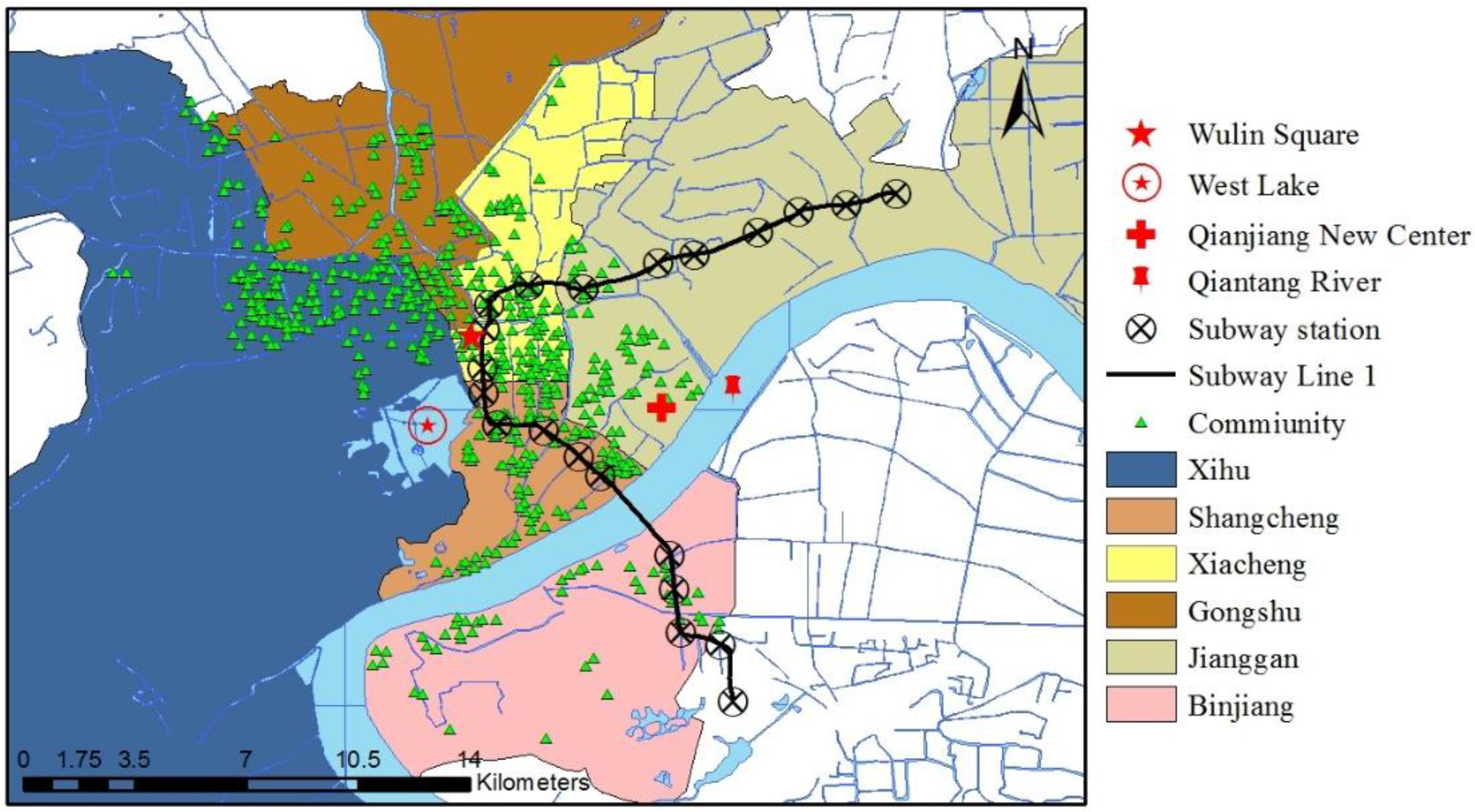
3.1. Study Area and Data Sources
3.2. Variable Selection
3.3. Empirical Model Specification
4. Results and Discussion
4.1. Results of Basic Models
4.2. Results of Quantile Regression Models
5. Conclusions
- (1)
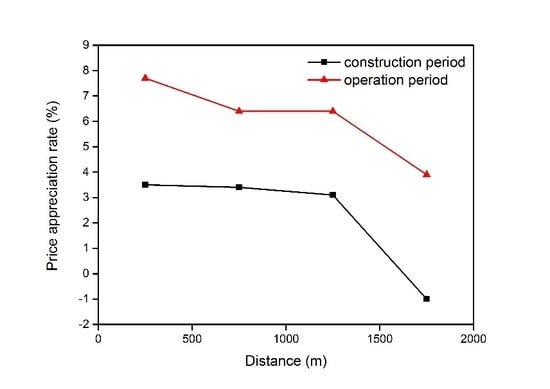
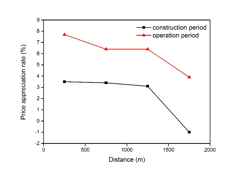
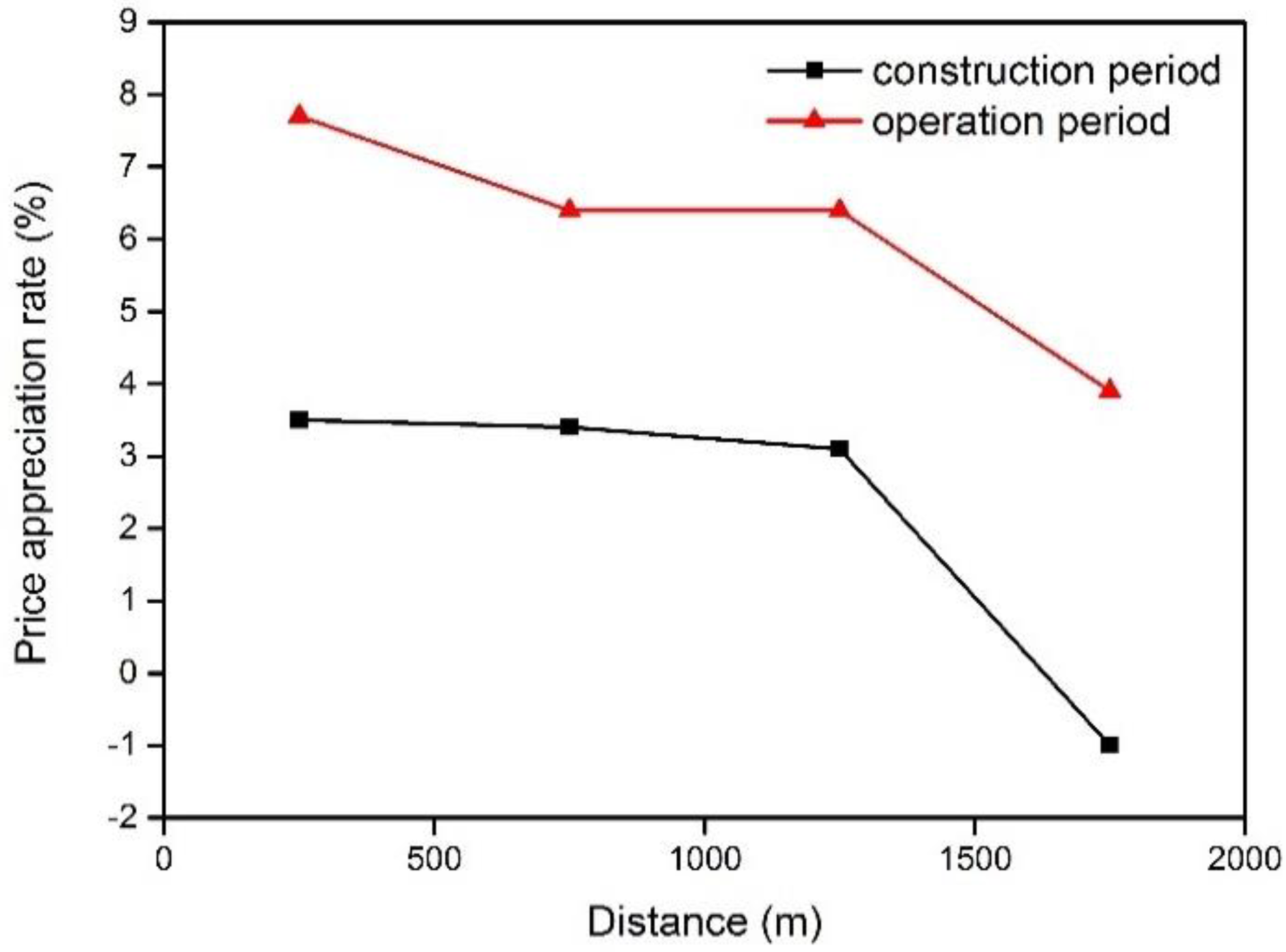
- The subway produces a significant impact on housing prices, and accessibility effects vary at different distance intervals. During construction and operation periods, housing prices are negatively related to subway distance, that is, every 1% decrease in subway distance results in a 0.049% increase in housing price. The value-added effect diminishes gradually with increasing distance. Specifically, houses within 500 m of a subway station enjoy the highest premium (6.2%). The appreciation rate experiences a sharp decline (2.1%) when the distance exceeds 1500 m.
- (2)
- The opening of the subway enhances the capitalization effect of subway accessibility. The subway has a significant and positive impact on housing prices in the construction and operation phases. First, the price elasticity of the distance variable increases from 0.044 during the construction period to 0.053 during the operation period. Second, the influence range of the subway also expanded from 1500 m to 2000 m. Finally, the percentage gain in housing prices during the operation period is higher than that during the construction period in each distance segment.
- (3)
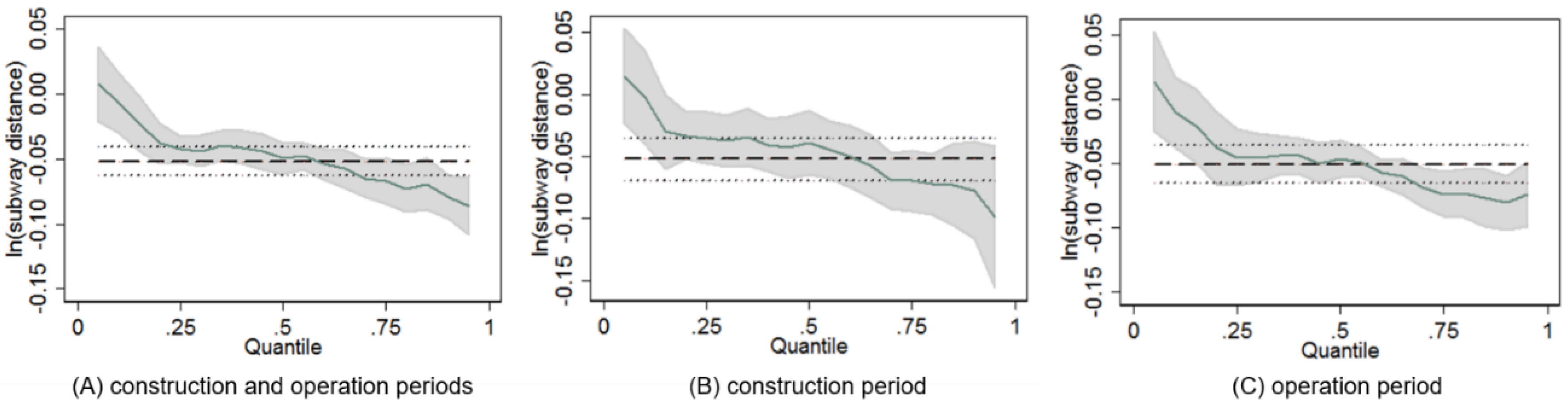
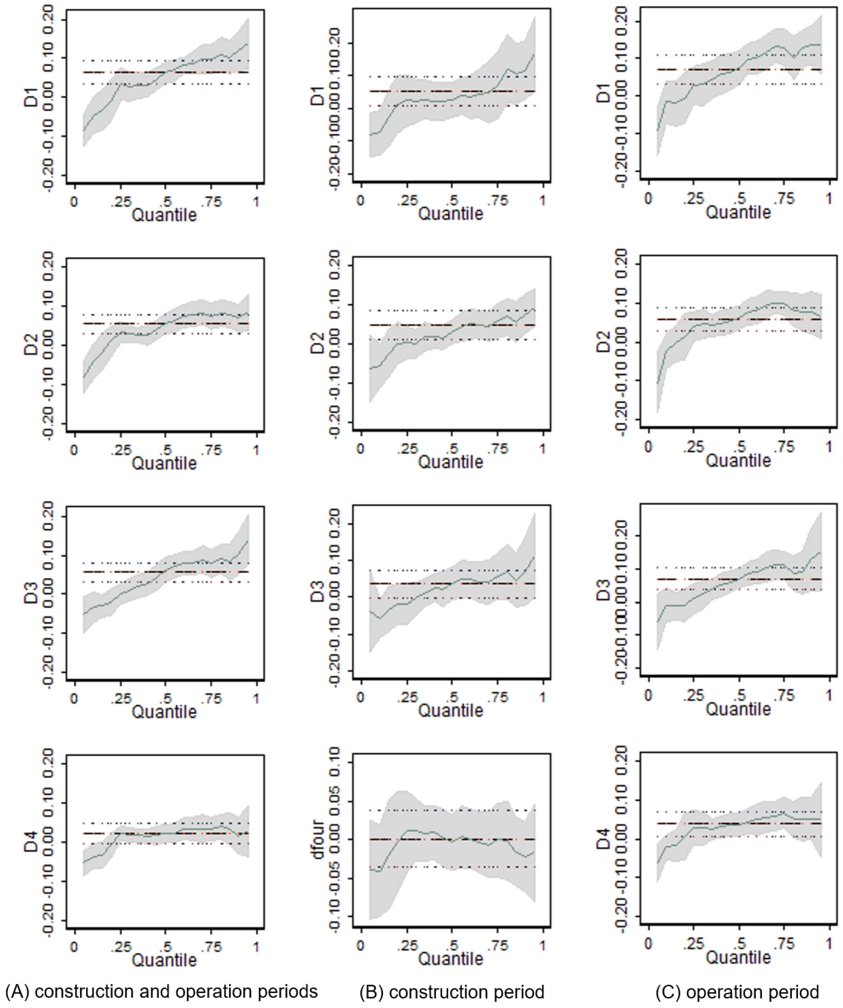
- The subway exhibits a heterogeneous capitalization effect across different houses of low, medium, and high prices. The quantile regression model further verifies results obtained from basic hedonic price models. Moreover, the quantile regression model also reveals that the subway produces evidently distinct impacts at different housing prices. The price elasticity (absolute value) of the subway distance exhibits a rising trend in conditional quantiles. Results indicate that medium- and high-priced communities are highly sensitive to rail transport accessibility. The effects of the subway in each distance segment also rise as housing prices increase in conditional quantiles. This finding suggests that the price premiums of medium- and high-priced houses are remarkably greater than that of low-priced houses.
- (4)
- The quantile regression model provides us with valuable information that cannot be obtained from the OLS regression and reveals the complex impacts of housing prices before and after the opening of the subway. From quantile regression results, we find that buyers of high-priced houses have different rail transit preferences from buyers of low-priced houses, thereby resulting in heterogeneity of the capitalization effect of the subway. By depicting the changing trend of implicit prices across the entire housing price distribution, quantile regression can comprehensively estimate subway impacts and reveal behavioral differences among home buyers at different price levels.
- (1)
- Strengthen the comprehensive development of land supply around subway stations. As an important development line and passenger corridor to the city, Hangzhou Subway Line 1 will promote the value of real estate around the station and affect the functional planning and layout of urban space. Drawing from the relevant conclusions of this study, the land around the station should implement comprehensive and high-intensity developments and give full play to the agglomeration function. Thus, the station area will form a functional area integrating public transportation, residential properties, commercial facilities, and office facilities, and then reflect the economic and social benefits of the urban rail transit.
- (2)
- Consider the potential for low-priced housing gentrification and avoid negative effects. Public transport is one of the important factors that influence the home purchasing decisions of people. The empirical analysis of Hangzhou Subway Line 1 finds that medium- and high-priced housing markets are sensitive to subway accessibility. Buyers of medium- and high-priced houses show a notable willingness to pay to live near a subway station. Hence, potential exists for the gentrification of low-priced houses surrounding the stations. Policymakers should fully consider this potential situation. In urban construction, policymakers should continue to improve urban infrastructure, ensure the supply of affordable housing, and formulate corresponding policies to secure housing affordability for the low-income population.
Author Contributions
Funding
Conflicts of Interest
Appendix A


References
- Voith, R. Changing Capitalization of CBD-oriented Transportation System: Evidence from Philadelphia, 1970-1988. J. Urban Econ. 1993, 33, 361–376. [Google Scholar] [CrossRef]
- Lewis-Workman, S.; Brod, D. Measuring the Neighborhood Benefits of Rail Transit Accessibility. Transp. Res. Rec. J. Transp. Res. Board 1997, 1576, 147–153. [Google Scholar] [CrossRef]
- Mcmillen, D.; Mcdonald, J. Reaction of House Prices to a New Rapid Transit Line: Chicago’s Midway Line, 1983–1999. Real Estate Econ. 2004, 32, 463–486. [Google Scholar] [CrossRef]
- Xu, T.; Zhang, M.; Aditjandra, P. The Impact of Urban Rail Transit on Commercial Property Value: New evidence from Wuhan, China. Transp. Res. Part A Policy Pract. 2016, 91, 223–235. [Google Scholar] [CrossRef]
- Zhang, M.; Meng, X.; Wang, L.; Xu, T. Transit Development Shaping Urbanization, Evidence from the Housing Market in Beijing. Habitat Int. 2014, 44, 545–554. [Google Scholar] [CrossRef]
- Nie, C.; Wen, H.; Fan, X. The Spatial and Temporal Effect on Property Value Increment with the Development of Urban Rapid Rail Transit: An Empirical Research. Geogr. Res. 2010, 29, 801–810. [Google Scholar]
- Yan, S.; Delmelle, E.; Duncan, M. The Impact of a New Light Rail System on Single-Family Property Values in Charlotte, North Carolina. J. Transp. Land Use 2012, 5, 60–67. [Google Scholar]
- Armstrong, R. Impacts of Commuter Rail Service as Reflected in Single-family Residential Property Values. Transp. Res. Rec. 1994, 1466, 88–98. [Google Scholar]
- Dubé, J.; Thériault, M.; Rosiers, F.D. Commuter Rail Accessibility and House Values: The Case of the Montreal South Shore, Canada, 1992–2009. Transp. Res. Part A 2013, 54, 49–66. [Google Scholar] [CrossRef]
- Bowes, D.; Ihlanfeldt, K. Identifying the Impacts of Rail Transit Stations on Residential Property Values. J. Urban Econ. 2001, 50, 1–25. [Google Scholar] [CrossRef]
- Nelson, A.; Mccleskey, S. Improving the Effects of Elevated Transit Stations on Neighborhoods; Transportation Research Record 1266; Transport Research Board: Washington, DC, USA, 1990. [Google Scholar]
- Sirmans, G.; Macpherson, D.; Zietz, E. The Composition of Hedonic Pricing Models. J. Real Estate Lit. 2005, 13, 3–43. [Google Scholar]
- Koenker, R.; Hallock, K. Quantile Regression. J. Econ. Perspect. 2001, 15, 143–156. [Google Scholar] [CrossRef]
- Dai, X.; Bai, X.; Xu, M. The Influence of Beijing Rail Transfer Stations on Surrounding Housing Prices. Habitat Int. 2016, 55, 79–88. [Google Scholar] [CrossRef]
- Liang, Q.; Kong, L.; Deng, W. Impact of URT on Real Estate Value: The Case of Beijing Metro Line 13. Econ. Geogr. 2007, 40, 98–103. [Google Scholar]
- Mei, Z.; Xu, S.; Liu, J. Spatio-temporal Effects of Guangzhou Metro 3rd Line on housing prices. Geogr. Sci. 2011, 7, 836–842. [Google Scholar]
- Wang, L. Empirical Study on the Impact of Urban Rail Transit on Housing Price-based on Hedonic Price Model. Areal Res. Dev. 2009, 28, 57–61. [Google Scholar]
- Ye, X.; Cai, W. Calculation Method of Urban Rail Transit Development Benefits. J. Tongji Univ. 2002, 30, 431–436. [Google Scholar]
- Zhang, W.; Li, H.; Duan, X. The Impacts of Rail Transit on Property Values-The Case of No.1 Line in Beijing. Econ. Geogr. 2012, 32, 46–51. [Google Scholar]
- Gu, J.; Jia, S. The Effects of Expected Transport Improvements on Housing Prices and Price Spatial Distribution-Hangzhou-Based Research Evidence of Planning the Mass Transit Railway. Econ. Geogr. 2008, 6, 1020–1024. [Google Scholar]
- Bajic, V. The Effects of a New Subway Line on Housing Prices in Metropolitan Toronto. Urban Stud. 1983, 20, 147–158. [Google Scholar] [CrossRef]
- So, H.; Tse, R.; Ganesan, S. Estimating the Influence of Transport on House Prices: Evidence from Hong Kong. J. Prop. Valuat. Invest. 1997, 15, 40–47. [Google Scholar] [CrossRef]
- Billings, S. Estimating the Value of a New Transit Option. Reg. Sci. Urban Econ. 2011, 41, 525–536. [Google Scholar] [CrossRef]
- Bae, C.; Jun, M.; Park, H. The Impact of Seoul’s Subway Line 5 on Residential Property Values. Transp. Policy 2003, 10, 85–94. [Google Scholar] [CrossRef]
- Haider, M.; Miller, E. Effects of Transportation Infrastructure and Location on Residential Real Estate Values, Application of Spatial Autoregressive Techniques. Transp. Res. Rec. J. Transp. Res. Board 2000, 1722, 1–8. [Google Scholar] [CrossRef]
- Pan, Q. The Impacts of an Urban Light Rail System on Residential Property Values: A Case Study of the Houston Metro Rail Transit Line. Transp. Plan. Technol. 2013, 36, 145–169. [Google Scholar] [CrossRef]
- Gatzlaff, D.; Smith, M. The Impact of the Miami Metrorail on the Value of Residences near Station Locations. Land Econ. 1993, 69, 54–66. [Google Scholar] [CrossRef]
- Cervero, R.; Landis, J. Assessing the Impacts of Urban Rail Transit on Local Real Estate Markets Using Quasi-experimental Comparisons. Transp. Res. Part A Policy Pract. 1993, 27, 13–22. [Google Scholar] [CrossRef]
- Lancaster, K. A New Approach to Consumer Theory. J. Political Econ. 1966, 74, 132–157. [Google Scholar] [CrossRef]
- Rosen, S. Hedonic Prices and Implicit Markets: Product Differentiation in Pure Competition. J. Political Econ. 1974, 82, 34–55. [Google Scholar] [CrossRef]
- Cervero, R.; Duncan, M. Transit’s Value-Added Effects: Light and Commuter Rail Services and Commercial Land Values. Transp. Res. Rec. J. Transp. Res. Board 2002, 1805, 8–15. [Google Scholar] [CrossRef]
- Debrezion, G.; Pels, E.; Rietveld, P. The Impact of Rail Transport on Real Estate Prices: An Empirical Analysis of the Dutch Housing Market. Urban Stud. 2006, 48, 997–1015. [Google Scholar] [CrossRef]
- Duncan, M. Comparing Rail Transit Capitalization Benefits for Single-Family and Condominium Units in San Diego, California. Transp. Res. Rec. J. Transp. Res. Board 2008, 2067, 120–130. [Google Scholar] [CrossRef]
- Efthymiou, D.; Antoniou, C. How Do Transport Infrastructure and Policies Affect House Prices and Rents? Evidence from Athens, Greece. Transp. Res. Part A Policy Pract. 2013, 52, 1–22. [Google Scholar] [CrossRef]
- Benjamin, J.; Sirmans, G. Mass Transportation, Apartment Rent and Property Values. J. Real Estate Res. 1996, 12, 1–8. [Google Scholar]
- Hess, D.; Almeida, T. Impact of Proximity to Light Rail Rapid Transit on Station-Area Property Values in Buffalo, New York. Urban Stud. 2014, 44, 1041–1068. [Google Scholar] [CrossRef]
- Agostini, C.; Palmucci, G. The Anticipated Capitalisation Effect of a New Metro Line on Housing Prices. Fisc. Stud. 2010, 29, 233–256. [Google Scholar] [CrossRef]
- Mathur, S.; Ferrell, C. Effect of Suburban Transit Oriented Developments on Residential Property Values; San José State University: San Jose, CA, USA, 2009. [Google Scholar]
- Royal Institution of Chartered Surveyors (RICS) Policy Unit. Land Value and Public Transport: Stage 1-Summary of Findings; Office of the Deputy Prime Minister: London, UK, 2002. [Google Scholar]
- Weinberger, R. Light Rail Proximity, Benefit or Detriment in the Case of Santa Clara County, California? Transp. Res. Rec. J. Transp. Res. Board 2001, 1747, 104–113. [Google Scholar] [CrossRef]
- Kate, K.; Cao, X. The Impact of Hiawatha Light Rail on Commercial and Industrial Property Values in Minneapolis. J. Public Transp. 2013, 16, 47–66. [Google Scholar]
- Knaap, G.; Ding, C.; Hopkins, L. Do Plans Matter? The Effects of Light Rail Plans on Land Values in Station Areas. J. Plan. Educ. Res. 2001, 21, 32–39. [Google Scholar] [CrossRef]
- Chen, H.; Rufolo, A.; Dueker, K. Measuring the Impact of Light Rail Systems on Single Family Home Values: A Hedonic Approach with GIS Application. Transp. Res. Rec. 1998, 73, 1–12. [Google Scholar]
- Huang, H. The Land-Use Impacts of Urban Rail Transit Systems. J. Plan. Lit. 1996, 11, 17–30. [Google Scholar] [CrossRef]
- Ryan, S. Property Values and Transportation Facilities: Finding the Transportation-land Use Connection. J. Plan. Lit. 1999, 13, 412–427. [Google Scholar] [CrossRef]
- Liu, K.; Wu, Q.; Wang, P. Econometric Analysis of the Impacts of Rail Transit on Property Values: The Number 1 and 2 Lines in Nanjing. Resour. Sci. 2015, 37, 133–141. [Google Scholar]
- Golub, A.; Guhathakurta, S.; Sollapuram, B. Spatial and Temporal Capitalization Effects of Light Rail in Phoenix from Conception, Planning, and Construction to Operation. J. Plan. Educ. Res. 2012, 32, 415–429. [Google Scholar] [CrossRef]
- Landis, J.; Guhathakurta, S.; Huang, W.; Zhang, M.; Fukuji, B. Rail Transit Investments, Real Estate Values and Land Use Change: A Comparative Analysis of Five California Rail Transit Systems; University of California Transportation Center Working Paper; University of California at Berkeley: Berkeley, CA, USA, 1995. [Google Scholar]
- Loomis, J.; Santiago, L.; Jesus, Y. Effects of Construction and Operation Phases on Residential Property Prices of the Caribbean’s First Modern Rail Transit System. Urban Public Econ. Rev. 2012, 17, 57–78. [Google Scholar]
- Pagliara, F.; Papa, E. Urban Rail Systems Investments: An Analysis of the Impacts on Property Values and Residents’ Location. J. Transp. Geogr. 2011, 19, 200–211. [Google Scholar] [CrossRef]
- Henneberry, J. Transport Investment and House Prices. J. Prop. Valuat. Invest. 1998, 16, 144–158. [Google Scholar] [CrossRef]
- Al-Mosaind, M.; Dueker, K.; Strathman, J. Light-Rail Transit Stations and Property Values: A Hedonic Price Approach; Transportation Research Record 1400; Transport Research Board: Washington, DC, USA, 1993. [Google Scholar]
- Debrezion, G.; Pels, E.; Rietveld, P. The Impact of Railway Stations on Residential and Commercial Property Value: A Meta-analysis. J. Real Estate Financ. Econ. 2007, 35, 161–180. [Google Scholar] [CrossRef]
- Dewees, D. The Effect of a Subway on Residential Property Values in Toronto. J. Urban Econ. 1976, 3, 357–369. [Google Scholar] [CrossRef]
- Grass, R. The Estimation of Residential Property Values around Transit Station sites in Washington, DC. J. Econ. Financ. 1992, 16, 139–146. [Google Scholar] [CrossRef]
- Voith, R. Capitalization of Local and Regional Attributes into Wages and Rents: Differences and Mixed-Use Communities. J. Reg. Sci. 1991, 31, 127–145. [Google Scholar] [CrossRef]
- Gu, Y.; Guo, R. The Impacts of the Rail Transit on Property Values: Empirical Study in Batong Line of Beijing. Econ. Geogr. 2008, 28, 411–414. [Google Scholar]
- Zhong, H.; Li, W. Rail Transit Investment and Property Values: An Old Tale Retold. Transp. Policy 2016, 51, 33–48. [Google Scholar] [CrossRef]
- Koenker, R.; Bassett, J. Regression Quantiles. Econom. J. Econom. Soc. 1978, 46, 33–50. [Google Scholar] [CrossRef]
- Koenker, R.; Bassett, J. Robust Tests for Heteroscedasticity Based on Regression quantiles. Econom. J. Econom. Soc. 1982, 50, 43–61. [Google Scholar] [CrossRef]
- Lin, Y.; Chang, C.; Chen, C. Why Homebuyers Have a High Housing Affordability Problem: Quantile Regression Analysis. Habitat Int. 2014, 43, 41–47. [Google Scholar] [CrossRef]
- Mak, S.; Choy, L.; Ho, W. Quantile Regression Estimates of Hong Kong Real Estate Prices. Urban Stud. 2010, 47, 2461–2472. [Google Scholar] [CrossRef]
- Mueller, J.; Loomis, J. Does the Estimated Impacts of Wildfires Vary with the Housing Price Distribution? A quantile Regression Approach. Land Use Policy 2014, 41, 121–127. [Google Scholar] [CrossRef]
- Zhang, L. Flood Hazards Impact on Neighborhood House Prices: A Spatial Quantile Regression Analysis. Reg. Sci. Urban Econ. 2016, 60, 12–19. [Google Scholar] [CrossRef]
- Zietz, J.; Zietz, E.; Sirmans, G. Determinants of House Prices: A Quantile Regression Approach. J. Real Estate Financ. Econ. 2008, 37, 317–333. [Google Scholar] [CrossRef]
- Kang, H.; Liu, S. The Impact of the 2008 Financial Crisis on Housing Prices in China and Taiwan: A Quantile Regression Analysis. Econ. Model. 2014, 42, 356–362. [Google Scholar] [CrossRef]
- Wang, Y.; Feng, S.; Deng, Z.; Cheng, S. Transit Premium and Rent Segmentation: A Spatial Quantile Hedonic Analysis of Shanghai Metro. Transp. Policy 2016, 51, 61–69. [Google Scholar] [CrossRef]
- Song, Y.; Zenou, Y. Urban Villages and Housing Values in China. Reg. Sci. Urban Econ. 2012, 42, 495–505. [Google Scholar] [CrossRef]
- Jiang, Y.; Ye, X.; Wang, Z. Impact Area of Shanghai Rail Transit Line 1 on Development Benefits. Urban Mass Transit 2007, 10, 28–31. [Google Scholar]
- Mohammad, S.; Graham, D.; Melo, P.; Anderson, R. A Meta-analysis of the Impact of Rail Projects on Land and Property Values. Transp. Res. Part A Policy Pract. 2013, 50, 158–170. [Google Scholar] [CrossRef]
- Cheshire, P.; Sheppard, S. Estimating the Demand for Housing, Land, and Neighbourhood Characteristics. Oxf. Bull. Econ. Stat. 1998, 60, 357–382. [Google Scholar] [CrossRef]
- Wen, H.; Bu, X.; Qin, Z. Spatial Effect of Lake Landscape on Housing Price: A Case Study of the West Lake in Hangzhou, China. Habitat Int. 2014, 44, 31–40. [Google Scholar] [CrossRef]
- Wen, H.; Jin, Y.; Zhang, L. Spatial Heterogeneity in Implicit Housing Prices: Evidence from Hangzhou, China. Int. J. Strateg. Prop. Manag. 2017, 21, 15–28. [Google Scholar] [CrossRef]
- Wen, H.; Xiao, Y.; Zhang, L. Spatial Effect of River Landscape on Housing Price: An Empirical Study on the Grand Canal in Hangzhou, China. Habitat Int. 2017, 63, 34–44. [Google Scholar] [CrossRef]
- Liu, G.; Hu, G. Impact Area and Timeliness of Rail Transit to Value of Property: Base on Demonstration Analysis about Chongqing Rail Transit 2nd Line. Urban Econ. 2007, 12, 86–90. [Google Scholar]
- Wen, H.; Zhang, Z.; Zhang, L. An Empirical Analysis of Spatial Effects of Housing Price Based on the Spatial Econometric Model: A Case Study of Hangzhou. Syst. Eng. Theory Pract. 2011, 31, 1661–1667. [Google Scholar]


| Author | Location | Tansit Type | Accessibility Variable | Size of Study Area | Key Results |
|---|---|---|---|---|---|
| Henneberry [51] | Sheffield, England | T | Straight-line distance | Not indicate | Property value impact of Supertram was negative during the construction period, but disappeared after the opening of the system. |
| Nie et al. [6] | Shenzhen, China | M | Shortest distance to the nearest station | 1 km | Property value impact of MRT was negative during the construction period, but shifted to positive after the opening of the system. |
| Yan et al. [7] | Charlotte, (NC), USA | L | Network distance | 1 mile | Property value impact of LRT was negative during the construction period, but shifted to positive after the opening of the system. |
| Nelson and Mccleskey [11] | Atlanta, USA | H | Straight-line distance | 1.25 miles | Positive impacts of rail transit system proximity on property values. |
| Bowes and Ihlanfeldt [10] | Atlanta, USA | M | Straight-line distance | 3 miles | Single-family houses within a quarter mile from stations sold for 19% less than houses beyond three miles. |
| Mcmillen and Mcdonald [3] | Chicago, USA | M | Distance to the nearest metro station | 1.5 miles | Property value appreciation range changed from 11.7% during construction period to 19.4% around the operation period. |
| Hess and Almeida [36] | Buffalo, (NY), USA | L | Straight-line and network distance | 0.5 mile | Property value increased in high-income station areas, but decreased in low-income station areas. |
| Mathur and Ferrell [38] | San Francisco, USA | L | Straight-line distance | 3 miles | Positive effects of single-family values found within half a mile radius of the Ohlone Chynoweth TOD. |
| Agostini and Palmucci [37] | Santiago, Chile | M | Straight-line distance | 1 km | Property value increased between 4.1% and 7.9% after construction was announced and between 3.9% and 5.4% after the location of the stations was identified. |
| Billings [23] | Charlotte, (NC), USA | L | Travel distance | 1 mile | Property values were 4.0% higher for single-family properties and 11.3% higher for condominiums than outside aone mile radius of LRT stations. |
| Pan [26] | Houston, USA | L | Straight-line distance | 3 miles | The opening of the line had positive effects on property values; Negative impacts are associated with properties located within a quarter mile of stops. |
| Dubé et al. [9] | Montreal, Canada | C | Walking distance and car driving time | Not indicate | Housing prices were higher within 1500 m than outside the 1500 m radius. |
| Zhang [5] | Beijing, China | B, L, M | Distance to the nearest station | 1 mile | The impact zone for MRT can extend to more than one mile from stations but only to half a mile for LRT. |
| Liu et al. [46] | Nanjing, China | M | Straight-line distance | 2 km | Positive impacts are found for houses located within 1.5 km to stations. |
| Xu et al. [4] | Wuhan, China | M | Road network and straight-line distance | 1 km | Property value increased 16.7% for the 0–100 m core area and approximately 8.0% within the 100–400 m radius. |
| Dai et al. [14] | Beijing, China | M | Distance to the nearest station | 2 km | Positive effects found; the influence scope of a transfer station on property values was 1200–1400 m, while that of the non-transfer station was within 1000 m. |
| Zhong and Li [58] | Los Angeles, USA | M, L | Distance to the nearest station | 3 miles | Proximity to mature rail transit stations was positive for multi-family property values, but negative for single-family properties; multi-family property values were higher within 1600 m than their counterparts located beyond 1600 m. |
| District | Mean | Minimum | Maximum | Std. Deviation |
|---|---|---|---|---|
| Xihu | 23,383.046 | 11,957.656 | 40,360.580 | 6245.878 |
| Xiacheng | 21,121.221 | 13,021.148 | 39,228.508 | 4105.430 |
| Shangcheng | 21,116.857 | 14,760.147 | 34,234.477 | 3867.221 |
| Jianggan | 20,147.465 | 9251.887 | 34,350.520 | 5162.274 |
| Gongshu | 17,503.769 | 11,014.712 | 34,005.770 | 3296.209 |
| Binjiang | 16,142.620 | 11,010.741 | 25,214.473 | 3034.882 |
| Minimum | Maximum | Mean | 0.1 | 0.2 | 0.3 | 0.4 | 0.5 | 0.6 | 0.7 | 0.8 | 0.9 | |
|---|---|---|---|---|---|---|---|---|---|---|---|---|
| Housing price | 9251.887 | 40,360.580 | 21,549.933 | 12,491.621 | 15,557.850 | 18,625.190 | 21,662.192 | 24,698.702 | 27,854.164 | 31,133.921 | 34,120.748 | 37,229.013 |
| 5% conf. | 11,651.818 | 14,721.326 | 17,807.810 | 20,918.030 | 24,038.97 | 27,145.031 | 30,317.252 | 33,458.140 | 36,516.098 | |||
| interval | 13,097.392 | 16,243.774 | 19,347.658 | 22,467.880 | 25,572.516 | 28,692.322 | 31,794.818 | 34,871.150 | 37,952.434 | |||
| Distance to subway | 0.105 | 10.339 | 2.809 | 4.118 | 4.537 | 2.877 | 2.654 | 2.009 | 1.760 | 1.798 | 1.725 | 1.815 |
| Distance to Wulin Square | 0.350 | 12.790 | 4.631 | 9.978 | 7.448 | 4.677 | 4.201 | 3.167 | 2.782 | 2.654 | 3.394 | 3.094 |
| Distance to West Lake | 0.300 | 13.100 | 4.096 | 8.941 | 6.485 | 4.347 | 3.486 | 2.921 | 2.729 | 2.074 | 2.062 | 2.349 |
| Distance to the Qiantang River | 0.095 | 16.532 | 5.995 | 5.056 | 7.121 | 6.3447 | 5.544 | 5.442 | 6.066 | 6.357 | 4.983 | 6.840 |
| External Environment quality | 1 | 5 | 3.120 | 2.907 | 3.164 | 3.210 | 3.040 | 3.083 | 3.094 | 3.167 | 3.462 | 3.044 |
| Inner environment quality | 1 | 5 | 3.210 | 3.372 | 3.199 | 3.121 | 3.124 | 3.224 | 3.236 | 2.867 | 3.46 | 3.304 |
| Transportation convenience | 1 | 5 | 3.090 | 1.837 | 2.289 | 2.853 | 3.231 | 3.682 | 3.670 | 3.867 | 3.846 | 3.870 |
| Security | 1 | 5 | 3.590 | 3.698 | 3.356 | 3.448 | 3.628 | 3.654 | 3.686 | 3.500 | 3.640 | 3.609 |
| Education facilities | 1 | 4 | 3.130 | 2.721 | 2.685 | 3.005 | 3.215 | 3.292 | 3.434 | 3.533 | 3.269 | 3.609 |
| Nearby universities | 0 | 1 | 0.600 | 0.209 | 0.438 | 0.541 | 0.626 | 0.677 | 0.793 | 0.800 | 0.731 | 0.783 |
| Building age | 1 | 37 | 14.130 | 9.767 | 11.637 | 14.924 | 14.890 | 15.125 | 13.972 | 15.667 | 13.846 | 14.957 |
| Variable | Variable Definition and Quantization | Expected Sign |
|---|---|---|
| Distance to subway | Straight-line distance between the community center and the nearest subway station (km) | - |
| D1 | 1 if the distance to subway is within 500 m; 0 otherwise | + |
| D2 | 1 if the distance to subway is within 500–1000 m; 0 otherwise | + |
| D3 | 1 if the distance to subway is within 1000–1500 m; 0 otherwise | + |
| D4 | 1 if the distance to subway is within 1500–2000 m; 0 otherwise | + |
| Distance to West Lake | Straight-line distance between the community center and the coast of West Lake (km) | - |
| Distance to Wulin Square | Straight-line distance between the community center and Wulin Square (km) | - |
| Distance to the Qiantang River | Straight-line distance between the community center and the coast of the Qiantang River (km) | - |
| External environment quality | Park, mountain, river, lake, green space within 1000 m from the community, each item is scored with 1, total is 5 | + |
| Inner environment quality | Environmental quality inside the community, including greening condition, sanitary condition, air quality and quiet degree, is divided into 5 degrees: quite bad, bad, common, good, very good, scored as 1–5, respectively | + |
| Transportation convenience | Transportation conditions around the community, Measured by total number of bus routes within 1000 m of the community, is divided into 5 degrees: quite poor, poor, common, good, and very good, scored as 1–5, respectively | + |
| Security | Security conditions inside and outside the community, is divided into 5 degrees: quite bad, bad, common, good, and very good, scored as 1–5, respectively | + |
| Education facilities | A high school, junior high school, elementary school, and kindergarten facility within 1000 m of the community is each scored as 1, with a total of 4 | + |
| Nearby universities | 1 if a university or college within 1000 m, 0 otherwise | + |
| Building age | The age of the building (year, transaction years minus actual built years) | - |
| Xihu | 1 if the community is in Xihu district; 0 otherwise | ? |
| Gongshu | 1 if the community is in Gongshu district; 0 otherwise | ? |
| Xiacheng | 1 if the community is in Xiacheng district; 0 otherwise | ? |
| Shangcheng | 1 if the community is in Shangcheng district; 0 otherwise | ? |
| Jianggan | 1 if the community is in Jianggan district; 0 otherwise | ? |
| Y2011–Y2015 | 1 if the house was procured at time t (in years); 0 otherwise, where t = 2011, 2012, …, 2015 | ? |
| Model 1 (2011–2015) | Model 2 (2011–2012) | Model 3 (2013–2015) | |||||||
|---|---|---|---|---|---|---|---|---|---|
| Unstandardized Coefficients | Standardized Coefficients | Unstandardized Coefficients | Standardized Coefficients | Unstandardized Coefficients | Standardized Coefficients | ||||
| Coef. | p-Value | Beta | Coef. | p-Value | Beta | Coef. | p-Value | Beta | |
| (Constant) | 10.106 *** | 0.000 | 10.012 *** | 0.000 | 10.190 *** | 0.000 | |||
| Ln(Distance to subway station) | −0.049 *** | 0.000 | −0.211 | −0.044 *** | 0.000 | −0.194 | −0.053 *** | 0.000 | −0.225 |
| Ln(Distance to Wulin Square) | −0.057 *** | 0.000 | −0.169 | −0.048 *** | 0.004 | −0.147 | −0.059 *** | 0.000 | −0.172 |
| Ln(Distance to West Lake) | −0.204 *** | 0.000 | −0.543 | −0.206 *** | 0.000 | −0.565 | −0.207 *** | 0.000 | −0.548 |
| Ln(Distance to the Qiantang River) | −0.090 *** | 0.000 | −0.429 | −0.084 *** | 0.000 | −0.411 | −0.092 *** | 0.000 | −0.436 |
| External environment quality | 0.013 *** | 0.001 | 0.046 | 0.019 *** | 0.001 | 0.070 | 0.009 ** | 0.064 | 0.032 |
| Inner environment quality | 0.056 *** | 0.000 | 0.233 | 0.056 *** | 0.000 | 0.243 | 0.054 *** | 0.000 | 0.221 |
| Transportation convenience | 0.007 ** | 0.007 | 0.041 | 0.011 *** | 0.009 | 0.061 | 0.005 | 0.135 | 0.030 |
| Nearby Universities | 0.028 *** | 0.000 | 0.061 | 0.030 *** | 0.001 | 0.068 | 0.028 *** | 0.000 | 0.062 |
| Education facilities | 0.006 | 0.101 | 0.021 | 0.004 | 0.467 | 0.014 | 0.007 | 0.137 | 0.025 |
| Security | −0.005 | 0.187 | −0.019 | −0.003 | 0.639 | −0.010 | −0.007 | 0.191 | −0.025 |
| Ln(Building age) | −0.068 *** | 0.000 | −0.181 | −0.057 *** | 0.000 | −0.183 | −0.086 *** | 0.000 | −0.193 |
| Xihu | 0.509 *** | 0.000 | 1.005 | 0.490 *** | 0.000 | 0.997 | 0.517 *** | 0.000 | 1.010 |
| Gongshu | 0.335 *** | 0.000 | 0.530 | 0.360 *** | 0.000 | 0.586 | 0.318 *** | 0.000 | 0.499 |
| Xiacheng | 0.244 *** | 0.000 | 0.422 | 0.283 *** | 0.000 | 0.505 | 0.220 *** | 0.000 | 0.379 |
| Shangcheng | 0.146 *** | 0.000 | 0.252 | 0.183 *** | 0.000 | 0.322 | 0.122 *** | 0.000 | 0.210 |
| Jianggan | 0.238 *** | 0.000 | 0.343 | 0.265 *** | 0.000 | 0.398 | 0.224 *** | 0.000 | 0.319 |
| Y2012 | −0.067 *** | 0.000 | −0.118 | −0.070 *** | 0.000 | 0.160 | |||
| Y2013 | −0.010 | 0.232 | −0.017 | ||||||
| Y2014 | −0.078 *** | 0.000 | −0.139 | −0.066 *** | 0.000 | −0.136 | |||
| Y2015 | −0.088 *** | 0.000 | −0.156 | −0.073 *** | 0.000 | −0.150 | |||
| Adjusted R2 | 0.693 | 0.715 | 0.681 | ||||||
| F | 289.836 *** | 150.095 *** | 184.390 *** | ||||||
| Model 4 (2011–2015) | Model 5 (2011–2012) | Model 6 (2013–2015) | |||||||
|---|---|---|---|---|---|---|---|---|---|
| Unstandardized Coefficients | Standardized Coefficients | Unstandardized Coefficients | Standardized Coefficients | Unstandardized Coefficients | Standardized Coefficients | ||||
| Coef. | p-Value | Beta | Coef. | p-Value | Beta | Coef. | p-Value | Beta | |
| (Constant) | 10.115 *** | 0.000 | 10.048 *** | 0.000 | 10.194 *** | 0.000 | |||
| D1 | 0.061 *** | 0.000 | 0.075 | 0.035 * | 0.066 | 0.044 | 0.077 *** | 0.000 | 0.095 |
| D2 | 0.053 *** | 0.000 | 0.095 | 0.034 ** | 0.027 | 0.064 | 0.064 *** | 0.000 | 0.115 |
| D3 | 0.052 *** | 0.000 | 0.075 | 0.031 * | 0.066 | 0.045 | 0.064 *** | 0.000 | 0.093 |
| D4 | 0.021 * | 0.056 | 0.026 | −0.010 | 0.543 | 0.044 | 0.039 *** | 0.006 | 0.048 |
| Ln(Distance to Wulin Square) | −0.085 *** | 0.000 | −0.251 | −0.081 *** | 0.000 | −0.249 | −0.087 *** | 0.000 | −0.256 |
| Ln(Distance to West Lake) | −0.200 *** | 0.000 | −0.532 | −0.202 *** | 0.000 | −0.556 | −0.201 *** | 0.000 | −0.531 |
| Ln(Distance to the Qiantang River) | −0.089 *** | 0.000 | −0.426 | −0.081 *** | 0.000 | −0.393 | −0.093 *** | 0.000 | −0.442 |
| External environment quality | 0.010 *** | 0.008 | 0.036 | 0.016 *** | 0.007 | −0.013 | 0.006 | 0.208 | 0.022 |
| Inner environment quality | 0.058 *** | 0.000 | 0.239 | 0.057 *** | 0.000 | 0.059 | 0.055 *** | 0.000 | 0.228 |
| Transportation convenience | 0.007 ** | 0.015 | 0.038 | 0.010 ** | 0.013 | 0.019 | 0.004 | 0.254 | 0.023 |
| Nearby universities | 0.025 *** | 0.000 | 0.054 | 0.026 *** | 0.005 | 0.059 | 0.025 *** | 0.002 | 0.054 |
| Education facilities | 0.008 ** | 0.049 | 0.026 | 0.005 | 0.344 | 0.057 | 0.009 * | 0.086 | 0.029 |
| Security | −0.008 ** | 0.039 | −0.030 | −0.006 | 0.328 | 0.246 | −0.010 ** | 0.048 | −0.038 |
| Ln(Building age) | −0.071 *** | 0.000 | −0.189 | −0.059 *** | 0.000 | −0.022 | −0.090 *** | 0.000 | −0.203 |
| Xihu | 0.481 *** | 0.000 | 0.948 | 0.448 *** | 0.000 | −0.188 | 0.497 *** | 0.000 | 0.973 |
| Gongshu | 0.312 *** | 0.000 | 0.493 | 0.323 *** | 0.000 | 0.914 | 0.303 *** | 0.000 | 0.476 |
| Xiacheng | 0.222 *** | 0.000 | 0.385 | 0.252 *** | 0.000 | 0.529 | 0.203 *** | 0.000 | 0.351 |
| Shangcheng | 0.153 *** | 0.000 | 0.263 | 0.186 *** | 0.000 | 0.451 | 0.133 *** | 0.000 | 0.228 |
| Jianggan | 0.251 *** | 0.000 | 0.361 | 0.277 *** | 0.000 | 0.329 | 0.237 *** | 0.000 | 0.338 |
| Y2012 | −0.065 *** | 0.000 | −0.116 | −0.067 *** | 0.000 | 0.417 | |||
| Y2013 | −0.009 | 0.276 | −0.016 | −0.155 | |||||
| Y2014 | −0.077 *** | 0.000 | −0.137 | −0.066 *** | 0.000 | −0.137 | |||
| Y2015 | −0.086 *** | 0.000 | −0.153 | −0.074 *** | 0.000 | −0.154 | |||
| Adjusted R2 | 0.683 | 0.707 | 0.676 | ||||||
| F | 241.115 *** | 122.727 *** | 154.692 *** | ||||||
| Model 7 (2011–2015) | Model 8 (2011–2012) | Model 9 (2013–2015) | ||||
|---|---|---|---|---|---|---|
| Coef. | p-Value | Coef. | p-Value | Coef. | p-Value | |
| OLS | −0.049 *** | 0.000 | −0.044 *** | 0.000 | −0.053 *** | 0.000 |
| q05 | 0.008 | 0.484 | 0.015 | 0.392 | 0.014 | 0.269 |
| q10 | −0.007 | 0.507 | −0.002 | 0.894 | −0.010 | 0.442 |
| q15 | −0.023 ** | 0.023 | −0.030 ** | 0.009 | −0.021 ** | 0.027 |
| q20 | −0.038 *** | 0.000 | −0.033 ** | 0.002 | −0.038 *** | 0.000 |
| q25 | −0.042 *** | 0.000 | −0.035 *** | 0.000 | −0.045 *** | 0.000 |
| q30 | −0.044 *** | 0.000 | −0.038 *** | 0.000 | −0.046 *** | 0.000 |
| q35 | −0.040 *** | 0.000 | −0.034 *** | 0.000 | −0.044 *** | 0.000 |
| q40 | −0.041 *** | 0.000 | −0.041 *** | 0.000 | −0.044 *** | 0.000 |
| q45 | −0.044 *** | 0.000 | −0.042 *** | 0.000 | −0.050 *** | 0.000 |
| q50 | −0.050 *** | 0.000 | −0.039 *** | 0.000 | −0.047 *** | 0.000 |
| q55 | −0.048 *** | 0.000 | −0.044 *** | 0.000 | −0.049 *** | 0.000 |
| q60 | −0.054 *** | 0.000 | −0.050 *** | 0.000 | −0.057 *** | 0.000 |
| q65 | −0.058 *** | 0.000 | −0.058 *** | 0.000 | −0.060 *** | 0.000 |
| q70 | −0.065 *** | 0.000 | −0.070 *** | 0.000 | −0.069 *** | 0.000 |
| q75 | −0.067 *** | 0.000 | −0.070 *** | 0.000 | −0.074 *** | 0.000 |
| q80 | −0.073 *** | 0.000 | −0.073 *** | 0.000 | −0.073 *** | 0.000 |
| q85 | −0.069 *** | 0.000 | −0.073 *** | 0.000 | −0.077 *** | 0.000 |
| q90 | −0.079 *** | 0.000 | −0.078 *** | 0.000 | −0.080 *** | 0.000 |
| q95 | −0.086 *** | 0.000 | −0.099 *** | 0.000 | −0.074 *** | 0.000 |
| Model 10 (2011–2015) | Model 11 (2011–2012) | Model 12 (2013–2015) | ||||||||||
|---|---|---|---|---|---|---|---|---|---|---|---|---|
| D1 | D2 | D3 | D4 | D1 | D2 | D3 | D4 | D1 | D2 | D3 | D4 | |
| OLS | 0.061 *** | 0.053 *** | 0.052 *** | 0.021 * | 0.035 * | 0.034 ** | 0.031 * | −0.010 | 0.077 *** | 0.064 *** | 0.064 *** | 0.039 *** |
| q05 | −0.085 *** | −0.082 ** | −0.051 ** | −0.052 ** | −0.081 *** | −0.063 ** | −0.039 | −0.040 | −0.093 ** | −0.106 ** | −0.060 * | −0.059 ** |
| q10 | −0.046 * | −0.040 ** | −0.034 * | −0.034 ** | −0.073 ** | −0.056 ** | −0.057 ** | −0.040 * | −0.016 | −0.025 | −0.009 | −0.020 |
| q15 | −0.034 | −0.017 | −0.030 ** | −0.031 ** | −0.029 | −0.024 | −0.033 | −0.020 | −0.020 | −0.003 | −0.013 | −0.014 |
| q20 | −0.010 | 0.010 | −0.020 ** | −0.008 | 0.013 | 0.002 | −0.019 | −0.004 | −0.005 | 0.012 | −0.011 | 0.007 |
| q25 | 0.034 | 0.034 ** | 0.001 | 0.024 * | 0.021 *** | 0.006 | −0.017 | 0.011 | 0.027 | 0.038 ** | 0.010 | 0.030 |
| q30 | 0.028 | 0.028 * | 0.010 | 0.018 * | 0.020 | 0.001 | −0.003 | 0.012 | 0.030 | 0.046 *** | 0.023 | 0.028 |
| q35 | 0.031 | 0.026 ** | 0.019 | 0.019 * | 0.027 | 0.018 | 0.011 | 0.008 | 0.042 * | 0.042 ** | 0.037 * | 0.026 * |
| q40 | 0.032 | 0.028 * | 0.029 ** | 0.016 | 0.020 | 0.019 | 0.027 | 0.009 | 0.057 ** | 0.049 *** | 0.050 ** | 0.033 ** |
| q45 | 0.047 ** | 0.039 ** | 0.042 ** | 0.018 | 0.022 | 0.016 | 0.022 | 0.002 | 0.063 ** | 0.054 *** | 0.062 ** | 0.037 ** |
| q50 | 0.063 *** | 0.057 *** | 0.063 *** | 0.025 * | 0.027 | 0.030 | 0.036 | −0.003 | 0.076 *** | 0.063 *** | 0.070 *** | 0.037 ** |
| q55 | 0.071 *** | 0.062 *** | 0.072 *** | 0.025 ** | 0.038 | 0.0045 ** | 0.050 * | 0.004 | 0.099 *** | 0.077 *** | 0.085 *** | 0.045 ** |
| q60 | 0.081 *** | 0.076 *** | 0.079 *** | 0.035 ** | 0.035 | 0.051 ** | 0.048 * | 0.001 | 0.103 *** | 0.083 *** | 0.092 *** | 0.052 ** |
| q65 | 0.088 *** | 0.079 *** | 0.081 *** | 0.034 ** | 0.045 | 0.050 ** | 0.041 | −0.004 | 0.118 *** | 0.097 *** | 0.106 *** | 0.057 ** |
| q70 | 0.098 *** | 0.083 *** | 0.089 *** | 0.036 *** | 0.049 | 0.044 ** | 0.040 | −0.007 | 0.133 *** | 0.101 *** | 0.113 *** | 0.059 ** |
| q75 | 0.099 *** | 0.074 *** | 0.079 *** | 0.035 ** | 0.071 ** | 0.060 ** | 0.057 ** | 0.000 | 0.131 *** | 0.099 *** | 0.111 *** | 0.069 ** |
| q80 | 0.109 *** | 0.080 *** | 0.090 *** | 0.040 ** | 0.121 *** | 0.070 ** | 0.068 ** | −0.001 | 0.103 *** | 0.082 ** | 0.087 ** | 0.051 * |
| q85 | 0.102 *** | 0.076 *** | 0.083 *** | 0.035 * | 0.106 ** | 0.056 ** | 0.047 | −0.016 | 0.127 *** | 0.076 *** | 0.089 ** | 0.051 ** |
| q90 | 0.118 *** | 0.070 ** | 0.104 ** | 0.018 | 0.114 ** | 0.076 *** | 0.070 ** | −0.023 | 0.135 *** | 0.075 *** | 0.129 *** | 0.054 |
| q95 | 0.137 *** | 0.085 *** | 0.138 ** | 0.030 | 0.166 ** | 0.093 ** | 0.112 ** | −0.017 | 0.137 *** | 0.065 ** | 0.152 *** | 0.050 |
© 2018 by the authors. Licensee MDPI, Basel, Switzerland. This article is an open access article distributed under the terms and conditions of the Creative Commons Attribution (CC BY) license (http://creativecommons.org/licenses/by/4.0/).
Share and Cite
Wen, H.; Gui, Z.; Tian, C.; Xiao, Y.; Fang, L. Subway Opening, Traffic Accessibility, and Housing Prices: A Quantile Hedonic Analysis in Hangzhou, China. Sustainability 2018, 10, 2254. https://doi.org/10.3390/su10072254
Wen H, Gui Z, Tian C, Xiao Y, Fang L. Subway Opening, Traffic Accessibility, and Housing Prices: A Quantile Hedonic Analysis in Hangzhou, China. Sustainability. 2018; 10(7):2254. https://doi.org/10.3390/su10072254
Chicago/Turabian StyleWen, Haizhen, Zaiyuan Gui, Chuanhao Tian, Yue Xiao, and Li Fang. 2018. "Subway Opening, Traffic Accessibility, and Housing Prices: A Quantile Hedonic Analysis in Hangzhou, China" Sustainability 10, no. 7: 2254. https://doi.org/10.3390/su10072254
APA StyleWen, H., Gui, Z., Tian, C., Xiao, Y., & Fang, L. (2018). Subway Opening, Traffic Accessibility, and Housing Prices: A Quantile Hedonic Analysis in Hangzhou, China. Sustainability, 10(7), 2254. https://doi.org/10.3390/su10072254