What Contributes to Regional Disparities of Energy Consumption in China? Evidence from Quantile Regression-Shapley Decomposition Approach

Abstract

Given the binding provincial goals of energy intensity reduction and total energy consumption control in China, the main purpose of this study is to analyze the regional disparities of energy consumption from the perspectives of energy consumption per capita (EP) and energy intensity (EI), as well as to propose differentiated energy conservation policies. In doing so, quantile regression and regression-based Shapley value decomposition are performed in the case of 30 provinces in China during 2000–2015. The results of quantile regression specify that the impact of each determinant on EP differs distinctly at different quantiles. Income has a positive effect on EP, conversely, industrial structure, population density and transportation infrastructure have negative effects on EP. Similarly, the effect of each influencing factor on EI presents distinct dynamic varying process at different quantiles. Industrial structure, FDI and technological progress have significantly negative effects on EI, while energy mix has a positive effect on EI. Furthermore, based on the results of median regression, the assessment of contributions of individual variables to regional disparities of energy consumption per capita and energy intensity (i.e., EPD and EID) is conducted by the Shapley value decomposition method. It is found that inequality in income level is the most important reason for EPD and its annual average contribution rate is 70%. In addition, differences in population density play an important role in explaining EPD, while the inequality in transportation infrastructure contributes little to EPD. By contrast, EID is mainly due to differences in technological progress, whose annual average contribution rate is up to 46%. Following technological progress, the inequalities of FDI and energy mix are also important factors accounting for EID. On the whole, the contribution of industrial structure or regional factors is always small. Then, this study explores the provincial energy-saving development path based on the actual conditions of all provinces.

1. Introduction

In recent years, climate change and air pollution have been increasingly prominent, which may be mainly attributable to substantial energy consumption. However, the increase in energy consumption is regarded as an inevitable cost of economic growth [1]. Since the economic reforms in 1978, China’s economy has entered a sharp booming. China has exceeded the United States in energy consumption and became the largest energy consumer in 2010 [2]. With China’s primary energy consumption growing at over 5.3% per annum during 2005–2015, China accounted for 23% of world total primary energy consumption in 2016, with the value of 3053 million tons oil equivalent. What’s more, China has remained the largest growth market for energy for the last 16 years [3]. According to the Energy Outlook 2035 [4], the share of China’s energy demand will increase from 23% in 2015 to 26% in 2035. In addition, environmental deterioration has been increasingly prominent due to extensive economic development in the past decades. As the byproducts of energy consumption, a mushrooming number of Greenhouse gases (GHG) have posed a serious threat to environment because of the greenhouse effect. In 2007, China surpassed the United States and became the largest carbon emitter in the world [5]. Against the background of China’s new normal, it is supposed to realize the importance and urgency of energy saving and consumption reduction. Because of large population and energy consumption, the per capita environment capacity is small in China; consequently, China is confronted with an urgent dilemma of resources and environment.

Energy consumption per unit of GDP (also called energy intensity) reflects energy utilization efficiency in the process of economic growth, which is also the measurement of low-carbon economy and an important indicator of China’s mitigation commitment. During the 13th Five-Year Plan period 2016–2020, China aims to decrease energy intensity by 15% for the whole economy [6]. Nevertheless, the decline in energy intensity is found to result in an increase in energy consumption [7]. The rebound effect of energy resource suggests the improvement of energy efficiency may lead to an increase in energy consumption [8,9]. It is not advisable to use no increase in total energy consumption as a measurement of sustainability [10]. Therefore, we can see China has formulated the dual control targets of energy intensity and total energy consumption [11]. Thus, every province has been allocated its own burden in terms of energy intensity reduction and energy consumption increment (see

Table A1. Provincial mandatory targets of energy intensity (EI) reduction and energy consumption (EC) increment during the 13th Five-Year period (2016–2020).

Province (No.)	EI reduction Target (%)	EC Increment (10,000 Tons)	Province (No.)	EI reduction Target (%)	EC Increment (10,000 Tons)
Beijing (1)	17%	800	Hubei (17)	16%	2500
Tianjin (2)	17%	1040	Hunan (18)	16%	2380
Hebei (3)	17%	3390	Guangdong (19)	17%	3650
Shanxi (4)	15%	3010	Guangxi (20)	14%	1840
Inner Mongolia (5)	14%	3570	Hainan (21)	10%	660
Liaoning (6)	15%	3550	Chongqing (22)	16%	1660
Jilin (7)	15%	1360	Sichuan (23)	16%	3020
Heilongjiang (8)	15%	1880	Guizhou (24)	14%	1850
Shanghai (9)	17%	970	Yunnan (25)	14%	1940
Jiangsu (10)	17%	3480	Shaanxi (26)	15%	2170
Zhejiang (11)	17%	2380	Gansu (27)	14%	1430
Anhui (12)	16%	1870	Qinghai (28)	10%	1120
Fujian (13)	16%	2320	Ningxia (29)	14%	1500
Jiangxi (14)	16%	1510	Xinjiang (30)	10%	3540
Shandong (15)	17%	4070	Tibet (31)	-	-
Henan (16)	16%	3540

Note: All data are collected from the State Council and data of Tibet is not found; the numbers in parentheses represent different provinces.

). These mandatory targets aim to save energy resources, reduce pollutants and greenhouse gas emissions from the source and promote changes in economic development patterns. In fact, a striking feature of energy use in China is that there are significant regional differences in terms of total energy consumption and energy intensity (hereafter, EI). For one thing, energy consumption is unevenly distributed, for example, Shandong had the highest level of energy consumption with the value of 37945 tons of coal equivalent in 2015, while the least energy consumption was recorded in Hainan with merely 1938 tons of coal equivalent. For another, on the whole, EI in Eastern China is distinctly lower than that in Central and Western China. Specially, EI was the lowest in Beijing (0.51 tons per 10,000 yuan) in 2015 and slightly larger level of EI was reported by Guangdong (0.69) and Jiangsu (0.71). However, Ningxia had the maximum EI of 2.96, which was almost six times larger than that of Beijing. Thus, designing energy saving policies requires knowledge of interprovincial inequalities of both energy intensity and energy consumption.

Recently, there are an increasing number of energy-related inequality studies, which involve cross-country inequalities of per capita carbon emissions [12], energy intensity [13,14], energy consumption per capita [15] and ecological footprint per capita [16,17]. These studies specify intensity indicator and per capita indicator are commonly used in inequality research. Duro et al. [15] apply a Theil index decomposition to inequality in energy consumption per capita and a variance decomposition to inequality in energy intensity levels among 16 OECD countries. Teixido-Figueras and Duro [18] perform regression-based inequality decomposition to investigate the contributions of determinants to the inequality among countries in natural resource consumption, which is measured by ecological footprint per capita. As interprovincial carbon inequality can be defined as the inequality of per capita carbon emissions among different provinces [19], in the present study, interprovincial energy consumption inequality is defined as the inequality of energy consumption per capita (hereafter, EP) among different provinces. In comparison to aggregate energy consumption closely correlated with regional size, EP in different provinces is more comparable. Moreover, ignorance of province size (by population) may overestimate the real inequality performance. Specifically, provincial aggregated data set (i.e., aggregated energy consumption) will conceal intra-provincial heterogeneity in terms of energy consumption at individual level and residents’ energy welfare changes. For example, energy consumption of Shandong is about seven times larger than that of Ningxia in 2015, while Ningxia’s EP is twice larger than that of Shandong.

It is assumed that inter-national patterns of inequality in energy consumption per capita/energy intensity would largely be paralleled on inter-provincial scale. Investigating interprovincial disparities of EP and EI (hereafter, EPD and EID) can provide important information for energy consumption projection and energy policy making. Thus, it is of great practical significance to study EPD and EID with respect to their formation mechanisms. Given the abovementioned, several important questions naturally arise. First, how can the interprovincial differences in EP/EI be measured accurately? Second, how can the heterogeneity of EP and EI be understood among different areas? In other words, why does EP or EI vary across different regions? Third, how can the contributions of individual determinants of EP (EI) to EPD (EID) be quantified? Fourth, with the knowledge of the causes of regional differences in EP and EI, what policies should be oriented to narrow the gaps of EP and EI among different regions? This study intends to extend the literature by resolving the four aforementioned issues. In doing so, we merge two traditions in energy-related literature: the analyses of determinants and the measure of inequalities. Accordingly, an integrated framework mainly developed in the income inequality literature is to be performed in a sample of 30 provinces in China during 2000–2015. Specifically, in terms of regression equations, the inequality in EI or EP is decomposed by the Shapley value decomposition method. In this study, quantile regression serves as the econometric model in this research and the results of median regression (at the 50% quantile) are specified as the estimated equations for inequality decomposition.

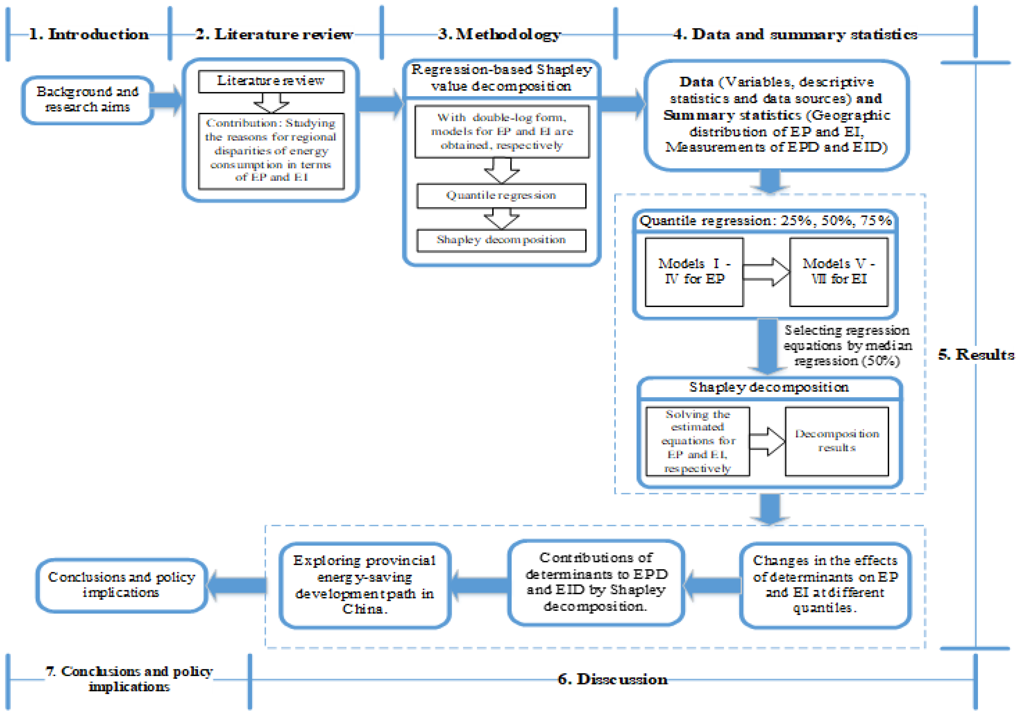
As shown in Figure 1, an integrated framework provides the clear research path of this study. Given that the provincial goals with respect to the integration of energy intensity reduction and energy consumption control, this research aims to extend the literature by finding the reasons for the disparities of EP and EI among provinces and ways to diminish these differences. Thus, in the case of 30 provinces in China, this study performs quantile regression and regression-based Shapley value decomposition developed in the income inequality literature. On the one hand, the quantile regression models for EP and EI are established, respectively. On the other hand, the estimated equations through median regression are selected for Shapley value decomposition. Accordingly, the contribution of each determinant to EPD or EID is got. In addition, provincial energy-saving development path is explored based on the actual situations of EP and EI in 2015. In the final part of the study, we present the conclusions and policy implications accordingly.

The rest of this research is organized as follows. Section 2 provides the literature review. Section 3 introduces the methodology. Section 4 presents the data and summary statistics. Section 5 presents the results of quantile regression and Shapley value decomposition. Section 6 discusses the results. The final section concludes this study and provides some policy implications.

2. Literature Review

Many countries have sought their ways to protect environment and conserve energy. In fact, since there are distinct differences in economic development, demographic indicators, energy utilization efficiency, geopolitical position and wealth of energy resources among different countries, energy consumption differs conspicuously as well. Accordingly, the international differences in energy consumption have generated abundant research interest and there are lots of studies on energy intensity convergence [20,21,22,23,24]. “Convergence” means decline in the differences of environmental indicator among countries, therefore, divergence in energy intensity indicates more attention should be paid to promoting knowledge diffusion in regions with high energy intensity [25]. Although international differences of energy use/intensity have attracted much concern, little attention has been paid to analyzing the reasons for these differences and these previous studies fail to quantify the contributions of individual determinants to these differences.

China’s provinces display considerable heterogeneity in economic development, population, technology and resource endowment [26,27], these factors may lead to different energy consumption patterns. Recently, studies on the heterogeneity analysis of energy consumption in China are increasingly found. Some scholars compare the effects of individual determinants on energy consumption among different areas through sub-sample regression. For example, using three groups of sample data, Li et al. [1] perform the random-effect model to investigate the effects of energy mix, economic structure and technical progress on energy intensity and find that each determinant presents different effects in three regions. Nevertheless, there exist some deficiencies in the previous studies. For one thing, traditional regional division, that is, eastern, central and western regions, is not suitable for all research issues; for another, the estimated coefficients through different sub-samples may suffer from incomparability. In addition, index decomposition analysis (IDA) method has also been employed by Jiang et al. [28] to decompose the difference between regional energy intensity and national average into pure energy intensity, industrial structure and export structure. However, it does not present the comprehensive inequality in energy intensity among provinces and fail to identify the contributions of decomposed effects to the interprovincial inequality in energy intensity.

Previous inequality research is mainly based on Lorentz curve [29], Gini coefficient [30], Theil index [12] or distributive tools [31]. Apart from these studies, regression model is also utilized in inequality research. The traditional regression methods focus on revealing the central tendency of conditional distribution (i.e., conditional mean) of dependent variable. For a long time, an overwhelming of attention has been paid to the central position of dependent variable, thereby cloaking scholars’ interest in non-central position (tail distribution). Quantile Regression depicts the shape of conditional distribution in non-central position by means of changes in quantiles [32]. This method of modeling the shape of conditional distribution is a breakthrough in inequality research field. Quantile regression has been widely applied to inequality related research, such as economic inequality in wage [33,34], education inequality in school quality [35] and health inequality in body weight [36]. Quantile regression provides a new perspective for energy policy makers to understand and narrow group differences under the given levels of energy consumption/energy intensity. In brief, quantile regression can resolve the following issues. Is the impact of each determinant on energy consumption/energy intensity different in different provinces? Hypothetically, what is the dynamic varying process of their effects presented in different provinces? In this study, quantile regression method is performed to provide evidence with regard to the differences in the effects of influencing factors on EP (EI) at different levels of EP (EI).

Combining the regression model with the inequality decomposition, Fields and Yoo [37] and Morduch and Sicular [38] propose a regression-based inequality decomposition method, which can identify and quantify the contributions of various determinants to total inequality. However, this approach is restricted to the form of regression function and the selection of inequality measure. In addition, the contributions of constant and residual terms are not handled properly. Shorrocks [39] develops an inequality decomposition framework based on the Shapley decomposition. Furthermore, Wan [40,41] proposes a framework that combines regression model with Shapley value decomposition of Shorrocks [39], which has effectively addressed the said deficiencies of traditional regression-based decomposition methods. Through the Shapley decomposition, inequality of the variable of interest can be decomposed into the contributions of individual determinants. In recent years, the regression-based decomposition has been increasingly utilized in energy-economics field [18,42,43]. Based on the OLS regression results, these studies attribute inequality measured by variance (i.e., R-squared or R2) to the contributions of individual variables. Rather, variance is rarely used as a measure of inequality because it is measured by absolute change instead of proportional change [44] and largely affected by the choice of measurement unit. In addition, these studies specify the regression models as semi-logarithmic forms. In fact, inequality is decomposed in terms of the logarithm of dependent variable rather than original variable, which may distort the decomposition results [40]. With no restriction imposed on the form of regression function and the measurement of inequality, the regression-based Shapley value decomposition approach can always be effective to obtain each determinant’s contribution to overall inequality.

To our best knowledge, no previous study has investigated energy consumption/energy intensity in China from the perspective of inter-provincial inequality. This study aims to provide adequate evidence with regard to the issue how to achieve provincial energy conservation targets of energy intensity reduction and energy consumption control. From the perspective of heterogeneity analysis, this paper investigates the determinants of EP (EI) with respect to changes in their effects on EP (EI) at different levels of EP (EI). In addition, we find the reasons for EPD (EID) and quantifies to what extent the determinants of EP (EI) contribute to interprovincial EPD (EID), thereby narrowing EPD and EID to achieve provincial and national energy conservation targets. Apart from previous studies, this research contributes to the literature in the following ways. (1) The existing literature cannot provide more detailed information about the characteristics of China’s energy consumption by using a single indicator. Given China’s dual control targets of energy intensity and total energy consumption, this study takes into account both energy consumption level and energy intensity. (2) Although previous studies have investigated the regional heterogeneity of energy consumption in China, little research has focused on achieving energy conservation by narrowing regional differences in energy consumption/energy intensity, which is a research gap to be filled in this study. In doing so, this paper performs the regression-based Shapley value decomposition, which has never been employed to study regional disparities of energy consumption before. (3) This paper performs quantile regression to explore several determining factors with respect to the changes in their effects on EP and EI at different quantiles, especially at the high and low quantiles. In addition, this method provides flexibility for studying a certain province with particular level of EP or EI, which is beyond the scope of mean regression model. (4) Following the results of median regressions, regression-based Shapley value decomposition proposed by Wan [40,41] is employed to identify the contributions of individual variables to inequalities (i.e., EPD and EID) measured by Gini coefficient, Theil index and mean logarithmic deviation. (5) Based on the combined econometric and decomposition analysis, this study enriches the application of inequality research method and extends the literature on energy-related issues. The analytical methods used in this paper not only reveal the differences in the impacts of each determinant on EP (EI) but also quantitatively attribute EPD and EID to the contributions of individual variables, thereby providing an in-depth understanding of conspicuous heterogeneity in EP and EI among different provinces.

3. Methodology

3.1. Quantile Regression

Quantile regression is proposed by Koenker and Bassett [32]. This approach can describe the entire picture of the conditional distribution of dependent variable rather than its conditional expectation. Based on the choice of quantile, it is feasible to employ quantile regression to model any position of the conditional distribution of dependent variable. The mean regression ignores some important information about the conditional distribution of dependent variable, such as non-central position, scale and skewness changes, which are the main limitations of mean regression. The above shortcomings can be well addressed by quantile regression. Moreover, quantile regression can deal with the heteroscedasticity and outliers and obtain more robust estimation results. In addition, quantile regression is applicable to asymmetrical distribution and thick-tailed distribution.

Let the distribution function of the continuous random variable $Y$ be $F\left(y\right)=P\left(Y\le y\right)$. For any $\mathsf{\tau }$ ranging from 0 to 1, the $\mathsf{\tau }$th quantile function of Y is defined as: $Q_y\left(\tau \right)=inf\left\{y:F_y\ge \tau \right\}$. The probability that $Y$ is less than $Q_y\left(\tau \right)$ is τ, which can be expressed as $\tau =P\left(Y\le Q_y\left(\tau \right)\right)$.

The basic model is described as:

$$y_{it}={\alpha }_i+{\displaystyle \sum }{X}_{it}{\beta }_i+u_{it}$$

(1)

${{\displaystyle \sum }}^{\text{}}{X}_{it}$ represents all the explanatory variables, ${\alpha }_i$ denotes the fixed effect and $u_{it}$ is the residual term. Specifically, the parameter estimates of model (1) at the $\mathsf{\tau }$th quantile, that is, ${\alpha }_i$, $\beta \left(\tau \right)$, can be obtained by solving the following function:

$$arg \begin{array}{c}min\\ \left({\alpha }_i, \beta \right)\end{array}{\displaystyle \sum }_{i=1}^N{\displaystyle \sum }_{t=1}^T{\rho }_{\tau }\left(y_{it}-{\alpha }_i-x_{it}\beta \right)$$

(2)

For quantile $\mathsf{\tau }$ ranging from 0 to 1, the test function ${\rho }_{\tau }\left(u\right)$ is formulated as:

$${\rho }_{\tau }\left(u\right)=u\left(\tau -I_{u<0}\right)=\tau u{I}_{\left[0，\infty \right)}\left(u\right)-\left(1-\tau \right)u{I}_{\left(-\infty , 0\right)}\left(u\right)$$

(3)

where $I_{u<0}()$ is an indicator function, this function is explained as follows. For $I_{\left[0，\infty \right)}\left(u\right)$, if $u\in \left[0,\infty \right)$, $I=1$; otherwise, $I=0$. Similarly, for $I_{\left(-\infty , 0\right)}\left(u\right)$, if $u\in \left(-\infty ,0\right)$, $I=1$; otherwise, $I=0$.

In this study, two different models are established to estimate the effects of several explanatory variables on EP and EI. In the first model for EP, variables are mainly selected from the perspective of final energy demand side, which is our main interest. The aggregate energy consumption is mainly from the industrial, commercial, household and transport sectors. Energy consumption in industrial sector is mainly correlated to industrial structure. Energy consumption in commercial and household sectors is mainly influenced by two factors. One is income level and the other is distribution characteristics of residents and businesses, such as population density which may promote the transition to low-carbon lifestyle and affect the “energy footprint”. Moreover, traffic energy consumption depends largely on convenience of public transportation; convenient transportation helps reduce energy consumption, while it may lead to the rapid growth of motor vehicles at the same time. Therefore, referring to the research of Chai [45], four main factors comprising income, industrial structure, population density and transportation infrastructure are introduced into the regression model of EP, which is specified by Equation (4).

Zheng et al. [46] conclude several internal and external factors of China’s economy that contribute to reducing energy intensity. Internal factors include technological progress, economic structure, enterprises’ ownership type, energy mix and energy policy; external factors (i.e., trade and FDI) represent China’s economic interactions with the outside world. Based on the studies of Li et al. [1] and Zheng et al. [46], this study identifies the effects of four main factor characterizing economic development on energy intensity, including three main internal factors and one external factor, thereby reflecting the energy efficiency of the whole economy. The second model for EI takes the following form shown in Equation (5).

It should be noted that urbanization is highly associated with GDP per capita [47,48,49], in addition, there is evidence to show that energy/electricity consumption causes urbanization [50]. Thus, urbanization is not included in Equations (4) and (5).

$$Ln{\mathrm{EP}}_{it}={\alpha }_0+{\alpha }_{1}Ln{\mathrm{GPC}}_{it}+{\alpha }_{2}Ln{\mathrm{IND}}_{it}+{\alpha }_{3}Ln{\mathrm{PD}}_{it}+{\alpha }_{4}Ln{\mathrm{INFRA}}_{it}+{\delta }_i+{\epsilon }_{it}$$

(4)

$$Ln{\mathrm{EI}}_{it}={\beta }_0+{\beta }_{1}Ln{\mathrm{EM}}_{it}+{\beta }_{2}Ln{\mathrm{IND}}_{it}+{\beta }_{3}Ln{\mathrm{FDI}}_{it}+{\beta }_{4}Ln{\mathrm{TP}}_{it}+{\delta }_i+{\epsilon }_{it}$$

(5)

where $i$ denotes the $i$th province ($i=1,2,3\cdots ,30$); $t$ represents the $t$th year; ${\mathrm{EP}}_{it}$ and ${\mathrm{EI}}_{it}$ signify energy consumption per capita and energy intensity, respectively, in province $i$ at time $t$; GPC, IND, PD, INFRA, EM, FDI and TP refer to GDP per capita, industrial structure, population density, transportation infrastructure, energy mix, foreign direct investment and technical progress, respectively. All variables are expressed in the form of natural logarithms. ${\epsilon }_{it}$ is random error term irrelevant to time and region. ${\delta }_i$ is the regional non-observed effect not changing with time, which specifies persistent regional differences among provinces, for example, different energy consumption characteristics caused by consumption habits, resources endowments and environmental regulations. Thus, regional dummy variables are introduced to capture the heterogeneity across regions. However, the degree of freedom may be easily lost in the case of 30 regional dummy variables. In addition, if the estimators of most dummy variables are insignificant, the validity of the models may be not robust accordingly. The traditional regional division in terms of administrative hierarchy or geographic location doesn’t objectively reflect the regional differences in energy consumption. Since China’s energy resources displays the feature of rich coal, lean petroleum and little natural gas, this paper divides 30 provinces into four categories based on the study of Zhang and Wang [51], in which regional classification is obtained according to the panel cluster analysis of energy consumption.

Table 1. Regional classification.

Category	Number	Provinces
Region 1	10	Hebei, Henan, Shanxi, Inner Mongolia, Liaoning, Hubei, Jiangsu, Shandong, Zhejiang, Guangdong
Region 2	7	Beijing, Shanghai, Heilongjiang, Shaanxi, Sichuan, Chongqing, Xinjiang
Region 3	10	Tianjin, Jilin, Gansu, Guizhou, Yunnan, Anhui, Hunan, Fujian, Jiangxi, Guangxi.
Region 4	3	Hainan, Qinghai, Ningxia

presents the classification results, accordingly, four regional dummy variables are introduced to Equations (4) and (5).

3.2. Shapley Value Decomposition

The regression-based Shapley decomposition method is originally developed in the income inequality literature [40,41,52]. This approach can be applied to any economic, social or development variables in addition to income [40] and it is used to study energy consumption related issues in this study, that is, identifying the contribution of each determinant to EPD and EID. Essentially, this method combines a regression model and the Shapley value decomposition approach proposed by Shorrocks [39]. The inequality of the variable of interest measured by Gini coefficient or other inequality indices (i.e., EPD or EID in this study), is attributable to individual determinants, constant term and residual term. Specially, this approach is applicative to any inequality measure and not restricted to a given functional form of regression model. Specifically, linear, semi-logarithmic and double-logarithmic forms are feasible and even interaction items can be included in regression model.

To illustrate the Shapley value decomposition procedure, we take energy consumption per capita (EP) for example. It is assumed that $Y=f\left(X,\mu \right)$ is the regression function of EP or its logarithm form. To simply demonstrate this approach, a linear regression model is specified for EP.

$$Y=\alpha +\beta X+\mu$$

(6)

where $\mathrm{X}=\left\{x_1,x_2,x_3,\cdots x_m\right\}$ denotes all determinants of EP included in the regression model, $\mathsf{\beta }$ = {${\beta }_1,{\beta }_2\cdots {\beta }_m$} represents parameter estimates of the $\mathrm{X}$ vector and $\mu$ is the residual term. Following the natural decomposition rule [39,44], we remove $\mu$ from Equation (6) and have

$$Y\left(\mu =0\right)=\widehat{Y}=\alpha +\beta X$$

(7)

Let G refer to the Gini operator, we apply G to both sides of Equation (7) and obtain $G\left(Y|\mu =0\right)=G(\widehat{Y})$. Hence, the contribution of $\mu$ to $G\left(Y\right)$ can be defined as:

$$C{O}_{\mu }=G\left(Y\right)-G(\widehat{Y})$$

(8)

$G(\widehat{Y})$ is attributable to the constant term and all determinants of EP, while $C{O}_{\mu }$ is associated with the residual term. That’s to say, the sum of $G(\widehat{Y})$ and $C{O}_{\mu }$ makes up the total inequality $G\left(\mathrm{Y}\right)$. Applying the natural decomposition rule to Equation (7), we obtain

$$\widehat{Y}\left(\alpha =0\right)=\tilde{Y}=\beta X$$

(9)

Then

$$G(\widehat{Y}|\alpha =0)=G(\tilde{Y})$$

(10)

The contribution of the constant term can be expressed as:

$$C{O}_{\alpha }=G(\widehat{Y})-G(\tilde{Y})$$

(11)

where $G(\tilde{Y})$ is attributed to all determinants in the vector $X$. The Shapley value decomposition method by Shorrocks [39] can be utilized to quantify the contributions of individual variables to $\mathrm{G}(\tilde{Y})$. Specially, compared with traditional methods, the approach of Shorrocks [39] is the only alternative when regression models are specified as the double-log form in Equations (4) and (5). The specific process of Shapley decomposition is presented as follows.

For Equation (9), let $x_1$ be evenly distributed among all provinces, we get its average value $\overline{x_1}$. Then, $\tilde{Y}$ can be formulated in the following form:

$$\tilde{Y}\left(x_1=\overline{x_1}\right)={\beta }_1{x}_1+{\displaystyle \sum }_{i=2}^m{\beta }_i·x_i$$

(12)

Then, we calculate corresponding $G{(\tilde{Y})}^{*}$ by using Equation (12). Accordingly, the difference $(G(\tilde{Y})-G{(\tilde{Y})}^{*})$ is defined as the contribution of $x_1$ to $G(\tilde{Y})$. In other words, $x_1$, which is equally distributed, makes no contribution to $G(\tilde{Y})$ and $G{(\tilde{Y})}^{*}$ is attributable to other determinants of EP (i.e., $x_2, x_3\cdots x_m$). Following this practice and the similar reasoning, we can identify the contributions of other individual variables to $G(\tilde{Y})$. The aforementioned procedure is not limited to Gini coefficient, rather, applicable to any inequality measure, including Theil index, Gini coefficient, variance, Atkinson index and mean logarithmic deviation.

4. Data and Summary Statistics

4.1. Data

Quantile regression and Shapley value decomposition are performed in a sample of 30 provinces over the period 2000–2015. The definition of all variables is shown in

Table 2. Definition of all variables.

	variables	Definition	Unit
Dependent variable	Energy intensity (EI)	Aggregate energy consumption/GDP	Tons per 10,000 yuan (at 2000 constant prices)
	Energy consumption per capita (EP)	Aggregate energy consumption/total population	Tons per person
Independent variable	Income (GPC)	GDP per capita	Yuan per person (at 2000 constant prices)
	Industrial structure (IND)	Added value of the tertiary industry/Added value of the secondary industry	%
	Population density (PD)	Total population/total area	person per square kilometers
	Transportation infrastructure (INFRA)	Area of paved roads by year end/total area	Square meters per square kilometers
	Foreign direct investment (FDI)	Amount of foreign direct investment actually utilized/GDP	%
	Energy mix (EM)	Coal consumption/Total energy consumption	%
	Technological progress (TP)	Patent applications granted	Number per year

. In order to eliminate price fluctuation, GDP per capita and EI are converted into 2000 constant prices. Compared with the tertiary industry, the secondary industry depends more on energy consumption because of energy-intensive industries. With industrial structural transformation in China, the share of added value of the secondary industry (including industrial and construction sectors) in GDP is falling; by contrast, the tertiary industry (including transport, commercial and other sectors) is increasing, while the share of the primary industry (i.e., agricultural sector) is relatively small. Therefore, it is feasible to use the ratio of added value in the tertiary industry to added value in the secondary industry as a measure of the advanced degree of industrial structure. The data used in this paper are mainly derived from China Statistical Yearbook [53], China Energy Statistical Yearbook [54] and China City Statistical Yearbook [55]. Specially, the data of FDI come from the provincial statistical yearbooks of local statistical bureaus.

Table 3. Descriptive statistics of all variables.

Statistics	LnEI	LnEP	LnGPC	LnIND	LnFDI	LnEM	LnPD	LnINFRA	LnTP
Mean	0.424	0.842	9.631	−0.153	0.539	4.16	5.671	6.507	8.549
Std. Dev	0.454	0.562	0.679	0.325	1.045	0.372	0.847	1.558	1.629
Min	−0.674	−0.586	7.88	−0.704	−2.684	2.497	2.372	2.116	4.248
Max	1.759	2.091	11.15	1.398	2.732	5.02	7.73	10.44	12.51
Skewness	0.503	−0.216	−0.0273	1.883	−0.605	−0.329	−0.449	−0.222	0.0520
Kurtosis	2.775	2.61	2.315	7.948	3.076	3.826	3.907	3.195	2.750
Jarque−Bera	21.23 ***	6.773 **	9.44 ***	773.3 ***	29.37 ***	22.28 ***	32.63 ***	4.715 *	1.463
Obs	480	480	480	480	480	480	480	480	480

Note: ***, ** and * denote the 1%, 5% and 10% significant levels, respectively.

presents the descriptive statistics of variables. The results of Jarque-Bera test show that almost all time-series variables follow non-normal distribution except LnTP, which indicates quantile regression is prior to OLS regression.

4.2. Summary Statistics

Figure 2 and Figure 3 plot the geographic distribution of China’s energy consumption in terms of energy consumption per capita (EP) and energy intensity (EI). As shown in Figure 2, EP was very unbalanced among different provinces. On the whole, the group of provinces with higher EP included Ningxia, Qinghai, Xinjiang, Inner Mongolia and Shanxi, with values ranging from 5.29 to 8.09 tons per capita. On the contrary, the least EP reported by Jiangxi was merely 1.85, slightly higher level of EP was reported by Anhui (2.01) and Guangxi (2.04). Figure 3 depicts the regional distribution of EI in 30 provinces in China, which demonstrates that EI in Eastern China was significantly lower than that in Central and Western China. Ningxia had the highest EI of 2.96 tons per 10,000 yuan, followed by Qinghai (2.74) and Xinjiang (2.58). By contrast, the lowest EI was recorded in some eastern coastal provinces, such as Beijing (0.51), Guangdong (0.69) and Jiangsu (0.71).

In order to fit inter-provincial EPD and EID, a general approach used in inequality literature is performed in this study. The Theil index (GE1), Gini coefficient and mean logarithmic deviation (i.e., MLD or GE0) are the most commonly utilized indicators as the measures of inequality since they are sensitive to changes in high, medium and low levels of the variable of interest, respectively. Therefore, the applications of these three indicators can get more comprehensive and objective information. When calculating these relative inequality indices, population shares and GDP shares serve as weights for EPD and EID, respectively. Accordingly, population-weighed and GDP-weighed inequality indices are obtained. The specific calculation methods are shown in Equations (13)–(18), where $x_i$ denotes EP in the $i$th province, $n$ represents 30 provinces, $u$ is the population-weighted average EP of all provinces and $p_i$ is the proportion of the $i$th province’s population in total population. $y_i$ represents EI in the $i$th province, $\mu$ is the GDP-weighted average EI of all provinces and $g_i$ is the share of the $i$th province’s GDP in total GDP. All resulting indices range from 0 to 1 and the value closer to 1 means higher inequality level (i.e., larger EPD or EID).

EPD is measured by using Equations (13)–(15). First, the Gini coefficient can be formulated as:

$$\mathrm{Gini}=\frac{{{\displaystyle \sum }}_{i=1}^n{{\displaystyle \sum }}_{j=1}^n\left|x_i-x_j\right|}{2n^{2}u} i=1,2\cdots ,30$$

(13)

Then, the generalized entropy indices (i.e., GE₁ and GE₀) are estimated. GE₁ is defined as:

$$\widehat{I}\left(\theta \right)={\mathrm{GE}}_1=\frac{1}{{{\displaystyle \sum }}_{i=1}^n{p}_i}{\displaystyle \sum }_{i=1}^n\frac{p_i{x}_i}{u}\log \left(\frac{x_i}{u}\right)\mathrm{if}\mathsf{\theta }=1$$

(14)

GE₀ can be expressed as:

$$\widehat{I}\left(\theta \right)=G{E}_0=\frac{1}{{{\displaystyle \sum }}_{i=1}^n{p}_i}{\displaystyle \sum }_{i=1}^n{p}_i\log \left(\frac{u}{x_i}\right)\mathrm{if}\mathsf{\theta }=0$$

(15)

Similarly, EPD is also measured following the preceding process, the Gini coefficient can be described as:

$$\mathrm{Gini}=\frac{{{\displaystyle \sum }}_{i=1}^n{{\displaystyle \sum }}_{j=1}^n\left|y_i-y_j\right|}{2n^2\mu }$$

(16)

GE₁ can be formulated as:

$$\check{I}\left(\theta \right)={\mathrm{GE}}_1=\frac{1}{{{\displaystyle \sum }}_{i=1}^n{g}_i}{\displaystyle \sum }_{i=1}^n\frac{g_i{y}_i}{\mu }\log \left(\frac{y_i}{\mu }\right)\mathrm{if}\mathsf{\theta }=1$$

(17)

GE₀ is given as:

$$\check{I}\left(\theta \right)={\mathrm{GE}}_0=\frac{1}{{{\displaystyle \sum }}_{i=1}^n{g}_i}{\displaystyle \sum }_{i=1}^n{g}_i\log \left(\frac{\mu }{y_i}\right)\mathrm{if}\mathsf{\theta }=0$$

(18)

The calculation results are plotted in Figure 4 and Figure 5. As can be seen from Figure 4, EPD of China’s 30 provinces estimated by three indicators presents similar varying trend for the period 2000–2015, which is also the case with EID in Figure 5. It can be found from Figure 4 that Gini coefficient, GE0 and GE1 were the maximal in 2001, which indicates EPD was the largest in 2001. EPD exhibited the trend of decrease from 2001 to 2010, while it remained stable with little change after 2010. As shown in Figure 5, the average values of GE0 and GE1 were 0.065 and 0.07, respectively; the average Gini coefficient was 0.201, while its maximum value (0.22) was recorded in 2001 and minimum value (0.186) was reported in 2013. On the whole, EID tended to decrease during 2001–2010, conversely, it increased slightly for the period 2010–2015.

5. Results

5.1. Results Through Quantile Regression

In quantile regression model, there are two competing methods for estimating the standard errors. One is bootstrapping and the other is the progressive variance-covariance matrix which is the default method of STATA. When the residual terms do not follow normal distribution and the iid hypothesis (independent and identically distributed), the bootstrapped standard errors are more robust [56]. Therefore, we employ the bootstrapping method to estimate standard errors. In bootstrapping, the seed is specified as 100 and the number of iterations is 1000. Three representative quantiles, that is, 25%, 50% and 75%, are selected for quantile regression estimates. The results of least square dummy variable model (LSDV) are provided for comparison. Considering that China’s provinces are not independent of one another, there may exist cross-sectional dependence accordingly; what’s more, group-wise heteroscedasticity should also be taken into account. Given the above-mentioned problems, LSDV can obtain the unbiased estimated coefficients but the standard errors are not robust [57]. Therefore, following Chen [57] and Herrerias et al. [58], the models are estimated by panel-corrected standard errors. In addition, given that there may exist multi-collinearity among explanatory variables, multi-collinearity test is conducted before the empirical analysis. For the regression model of EP, the VIF values of LnGPC, LnIND, LnPD and LnINFRA are 1.88, 1.09, 2.41 and 3.64, respectively. For the regression model of EI, the VIF values of LnEM, LnIND, LnFDI and LnTP are 1.65, 1.47, 1.30 and 1.16, respectively. All these VIF values are far smaller than 10, which indicates there is no multi-collinearity problem in both data sets.

As shown in

Table 4. Determinants of EP through LSDV and quantile regression.

Variables	Energy Consumption Per Capita (EP)
	Model I	Model II	Model III	Model IV
	Mean	25%	50%	75%
LnGPC	0.784 ***	0.940 ***	0.758 ***	0.688 ***
	(0.024)	(0.030)	(0.078)	(0.042)
LnIND	−0.277 ***	−0.255 ***	−0.219 ***	−0.269 ***
	(0.040)	(0.057)	(0.072)	(0.099)
LnPD	−0.121 ***	−0.008	−0.212 **	−0.144 ***
	(0.019)	(0.031)	(0.085)	(0.032)
LnINFRA	−0.067 ***	−0.196 ***	−0.010	0.009
	(0.014)	(0.023)	(0.068)	(0.022)
Constant	−5.604 ***	−7.114 ***	−5.236 ***	−4.851 ***
	(0.218)	(0.312)	(0.795)	(0.399)
Obs	480	480	480	480

Note: ***, ** and * denote p < 0.01, p < 0.05 and p < 0.1, respectively. The figures in parentheses are standard errors; quantile regression reports bootstrapped standard errors; LSDV reports panel-corrected standard errors. Quantile 25% denotes lower EP and quantile 75% indicates higher EP.

and

Table 5. Determinants of EI through LSDV and quantile regression.

Variables	Energy Intensity (EI)
	Model V	Model VI	Model VII	Model VIII
	Mean	25%	50%	75%
LnEM	0.286 ***	0.202 ***	0.258 ***	0.368 ***
	(0.030)	(0.072)	(0.052)	(0.042)
LnIND	−0.178 ***	−0.195 ***	−0.140 ***	−0.070
	(0.035)	(0.060)	(0.046)	(0.063)
LnFDI	−0.141 ***	−0.141 ***	−0.121 ***	−0.107 ***
	(0.010)	(0.016)	(0.013)	(0.019)
LnTP	−0.155 ***	−0.125 ***	−0.157 ***	−0.184 ***
	(0.009)	(0.015)	(0.012)	(0.012)
Constant	0.689 ***	0.589	0.804 ***	0.740 ***
	(0.168)	(0.371)	(0.233)	(0.247)
Obs	480	480	480	480

Note: ***, ** and * denote p < 0.01, p < 0.05 and p < 0.1, respectively. The figures in parentheses are standard errors; quantile regression reports bootstrapped standard errors; LSDV reports panel-corrected standard errors. Quantile 25% denotes lower EI and quantile 75% indicates higher EI.

, Column 2 presents the results through LSDV, while Columns 3–5 report the results through quantile regression. It can be seen that the estimated coefficients through LSDV and the quantile regression are homogeneous in most cases, which specify that the influence of each variable is relatively robust throughout the conditional distribution of dependent variable. In addition, the elastic coefficient of each determinant presents distinct varying process at different quantiles. That is to say, quantile regression provides more detailed description of changes in the impact of each variable on EP (EI) within the conditional distribution of EP (EI), which provides an in-depth understanding of conspicuous heterogeneity in EP and EI among different provinces.

According to the result through LSDV in Table 4, the estimated coefficients of all variables are significant at the 1% level. Industrial structure, population density and transportation infrastructure have negative impacts on EP, by contrast, GDP per capita has a positive impact on EP, which indicates energy consumption level has significantly risen with the increase of income. Moreover, it can be seen that the elastic coefficient of GDP per capita is less than unity, which indicates income contributes to the decrease of energy intensity. The developments of economy and society are usually accompanied by knowledge renewal and technology investment, thereby resulting in technological advance and improvement of energy efficiency. As shown in Table 5, all coefficients through LSDV are significant at the 1% level. The result shows industrial structure, FDI and technological progress have negative effects on EI, while energy mix has a positive effect on EI.

5.2. Results through Shapley Value Decomposition

5.2.1. Determining the Estimated Equations

Before the Shapley decomposition, it is necessary to determine the regression equations of original EP and EI. Median regression is a special case of quantile regression (at the 50% quantile). It uses the least absolute deviation estimate rather than the least squares estimate to describe the central tendency of the distribution of dependent variable. The median and mean value both aim to model the central location of the distribution of dependent variable. When the distribution of dependent variable is skewed, or there exists heteroscedasticity and outliers, the median is more applicable than the mean value to depict the distribution center. Therefore, for the following decomposition procedure, we choose the results by median regression to conduct the regression-based Shapley decomposition.

It should be noted that the objective of this study is to investigate the regional disparities in EP and EI rather than $Ln\mathrm{EP}$ and $Ln\mathrm{EI}$. Thus, solving the regression equations following Model III and Model VII, we obtain:

$$\exp \left({\delta }_i\right)·\exp \left({\epsilon }_{it}\right)$$

(19)

$$\mathrm{EI}=\exp \left(0.804\right)·\exp \left(0.258Ln\mathrm{EM}-0.140Ln\mathrm{IND}-0.121Ln\mathrm{FDI}-0.157Ln\mathrm{TP}\right)·\exp \left({\delta }_i\right)·\exp \left({\epsilon }_{it}\right)$$

(20)

Based on Equations (19) and (20), EPD (EID) is estimated by using the original EP (EI) not the natural logarithm of EP (EI). In addition, it should be noted that EPD and EID are gauged by relative indices, that is, Gini coefficient, GE1 and GE0, as shown in Section 4.2. These indices conform to homogeneity, in other words, the constant term does not contribute to total inequality because the constant term is a scalar and can be removed without affecting inequality index. Accordingly, the final equations are given as:

$$\mathrm{EP}=\exp \left(0.758Ln\mathrm{GPC}-0.219Ln\mathrm{IND}-0.212Ln\mathrm{PD}-0.01Ln\mathrm{INFRA}+\mathrm{REG}\right)$$

(21)

$$\mathrm{EI}=\exp \left(0.258Ln\mathrm{EM}-0.140Ln\mathrm{IND}-0.121Ln\mathrm{FDI}-0.157Ln\mathrm{TP}+\mathrm{REG}\right)$$

(22)

where REG is the new indicator constructed by regional dummy variables. This paper employs the commonly used method in previous research [59,60] which combines the regional dummy variables to represent regional factors impact. The contribution of the residual can be obtained according to the study of Wan [40], as illustrated in Section 3.2. The total inequality is attributed to the residual term and all independent variables and the explained proportion by independent variables is obtained by solving $100\times \left(1-\frac{\left|\mathrm{residual}\right|}{\mathrm{Gini}}\right)$ [60].

Table 6. The explained proportions by independent variables in EPD and EID.

Year	EPD				EID
	Gini	Independent Variables	Residual	Explained Proportion	Gini	Independent Variables	Residual	Explained Proportion
2000	0.238	0.194	0.044	81.5%	0.211	0.150	0.061	71.1%
2001	0.245	0.206	0.039	84.0%	0.220	0.159	0.061	72.1%
2002	0.242	0.204	0.038	84.3%	0.208	0.167	0.041	80.2%
2003	0.235	0.230	0.005	97.8%	0.220	0.179	0.041	81.5%
2004	0.222	0.231	0.009	96.0%	0.217	0.176	0.041	81.0%
2005	0.215	0.224	0.009	95.7%	0.206	0.172	0.034	83.5%
2006	0.214	0.234	0.020	90.7%	0.208	0.172	0.036	82.6%
2007	0.212	0.234	0.022	89.6%	0.205	0.168	0.037	82.0%
2008	0.207	0.226	0.019	90.6%	0.194	0.173	0.021	88.9%
2009	0.200	0.220	0.020	90.1%	0.193	0.180	0.013	93.5%
2010	0.192	0.200	0.008	95.9%	0.188	0.184	0.004	97.8%
2011	0.191	0.193	0.002	99.2%	0.189	0.183	0.006	96.9%
2012	0.190	0.186	0.004	97.9%	0.190	0.184	0.006	96.9%
2013	0.193	0.181	0.012	93.9%	0.186	0.180	0.007	96.5%
2014	0.189	0.180	0.009	95.2%	0.187	0.178	0.009	95.2%
2015	0.190	0.179	0.011	94.3%	0.188	0.176	0.012	93.8%
Mean	0.211	0.208	0.017	92.3%	0.201	0.174	0.027	87.1%

shows that on average all independent variables in Model III play 92.3% contribution role to EPD by using Gini coefficient as inequality measure, while in Model VII 87.1% to EID. That’s to say, about 90% of EPD or EID can be explained by the selected explanatory variables in Model III or Model VII. The impact of the residual term is relatively little, which indicates the modelling is valid and the policy implications can be forceful and convincing. Accordingly, Equations (21) and (22) are suitable for the following decomposition process.

5.2.2. Decomposition Results in Different Years

In the preceding section, the contribution of the residual term has been identified. In order to identify the contributions of individual determinants to EPD and EID measured by Gini, GE0 and GE1 obtained in Section 4.2, the Shapley value method proposed by Shorrocks [39] is the only alternative. As the explained inequality by all determinants is denoted by $G(\tilde{Y})$ shown in Section 3.2, $G(\tilde{Y})$ according to Equations (21) and (22) is specified as denominator to calculate the relative contribution rate of each determinant to $G(\tilde{Y})$. Accordingly, the sum of the contribution rates of all determinants is 100%. The results of Shapley value decomposition are shown in Figure 6, Figure 7, Figure 8, Figure 9, Figure 10 and Figure 11. As is mentioned in Section 3.2, if a certain determinant $x_1$ is equally distributed among regions, it would make no contribution to inequality according to Shapley value decomposition. For the explanation of decomposition results, the contribution of the $i$th determinant $x_i$ is obtained by quantifying its effect on total inequality if $x_i$ is evenly distributed among all provinces or removed. Specifically, EPD is attributable to inequalities in income, industrial structure, population density, transportation infrastructure and regional factors among 30 provinces.

As shown in Figure 6, Figure 7 and Figure 8, EPD is mainly due to interprovincial inequality of income, whose annual average contribution rate is up to 70–81%. However, the inequality in transportation infrastructure plays a role in reducing EPD over the analyzed period, although the absolute value of its annual average contribution rate is smaller than 1% according to Figure 6. The second largest contributor to EPD is the inequality in population density, following by the inequalities in population density and regional factors. In addition, the inequality in industrial structure makes little contribution to EPD, the absolute value of its annual average contribution rate is no larger than 2.5%.

From Figure 9, Figure 10 and Figure 11, differences in technological progress are the most important factor in explaining EID, whose annual average contribution rate is about 50%. Following technological progress, inequality in FDI plays a prominent role in explaining EID, its contribution rate presents the trend of decrease, which indicates the reduction in the inequality in FDI between provinces. Furthermore, the inequality in energy mix is also an important reason for EID. It should be noted that the contribution rates of both industrial structure and regional factor are quite small.

6. Discussion

6.1. Changes in the Effects of Determinants on EI and EP at Different Quantiles

Table 4 presents the impacts of various variables on EP through quantile regression. It is found that the elastic coefficient of each determinant fluctuates distinctly at different quantiles. The elastic coefficient of income is significantly positive at the 25%, 50% and 75% quantiles, which indicates that income has a positive impact on EP within the entire conditional distribution of EP. The positive effect of income decreases with EP rising, that’s to say, income in high-EP areas has a smaller positive effect on EP than low-EP areas. It is believed that the increase of income will improve consumption level, thereby leading to the increase in energy consumption. In low-EP areas, energy demand has not been fully met, thus, the driving strength of income on energy consumption is relatively large. By contrast, in high-EP areas, energy demand has been well met. Given the diminishing marginal effects, the stimulating effect of income is smaller.

The elastic coefficient of industrial structure is significantly negative at all quantiles, which specifies that industrial structure is an important factor to reduce energy consumption. Its elastic coefficient fluctuates slightly at different quantiles, thus, the negative effect of industrial structure on EP is quite robust and stable in different provinces. Thus, it is imperative to accelerate the optimization and upgrading of industrial structure. With China’s economy entering “new normal”, traditional extensive economic growth must be changed. The economic restructuring is not only the inevitable choice of sustainable economic development but also an effective measure for energy conservation and consumption reduction.

Population density has a negative effect on EP, which indicates population density contributes to decreasing energy consumption and this finding conforms to the study of Otsuka [61] in Japanese residential sector. The effect of population density on EP is not significant at the 25% quantile, which suggests population density in high-EP areas is more effective in energy intensive utilization than low-EP areas. In some high-EP provinces, such as Xinjiang, Qinghai, Inner Mongolia and Ningxia with small population and abundant resources, the increase of population density leads to marginal decreasing effect of energy consumption. In other high-EP provinces, such as Jiangsu, Beijing and Shanghai with large population and advanced economies, high population density promotes the development public transportation, facilities and infrastructures, thereby reducing energy consumption in transportation and household sectors.

It is found that transportation infrastructure has a negative effect on EP. This is mainly because dense transportation network is conducive to optimizing the distribution of energy resources and the combination of inputs to improve the production efficiency of enterprises. The elastic coefficient of transportation infrastructure is only significant at the 25% quantile. In fact, with the increase in energy consumption level mainly caused by economic growth, the number of vehicles has increased as well, thereby the negative effect of transportation infrastructure is gradually counteracted.

Table 5 shows the effects of various variables on EI through quantile regression. The effect of each determinant presents dynamic varying process at different quantiles. To clarify these changes, we should first observe the regional distribution characteristics of EI (see Figure 3). EI is the highest in Western China, followed by the Central and Eastern China. This distribution feature is highly in line with the level of development in China. Generally, compared with high-EI areas, low-EI areas have high proportion of coal consumption, advanced technological level, optimized industrial structure and more FDI inflows.

Energy mix has a positive impact on EI at different quantiles and the elastic coefficient of energy mix presents a trend of increase with quantile increasing, which indicates energy mix in high-EI areas has a larger positive effect on EI than low-EI areas. It is because that in high-EI areas the share of coal consumption is higher, moreover, coal is not utilized in an advanced and clean way due to technical limitations.

Industrial structure has a negative effect on EI, which suggests that the transformation of industrial structure is conducive to reducing EI. However, this effect is insignificant at the 75% quantile, it is because high-EI areas are in the stage of industrialization, economic development depends more on energy-intensive industries than the service industry, furthermore, industrial structure optimization is not high on the agenda. Therefore, it is particularly urgent for low-EI regions to optimize and upgrade their economic structure, one way to do this is to promote high-energy consumption and low value-added industries transferring from the Eastern China to Central and Western China.

FDI has a negative effect on EI at different quantiles. It is because technology spillovers of FDI contribute to reducing EI [62]. The negative effect of FDI is the lowest at the 75% quantile, which specifies that the effect of FDI has been offset to some extent in high-EI regions. It results from that high-EI areas, mainly concentrated in Central and Western China (see Figure 3), have introduced much foreign investments with the acceleration of openness in recent years. However, because of mild environmental regulations, much high energy-consuming multinational companies have been attracted (also called “pollution paradise” effect), which offsets partial technology spillover effect of FDI on EI.

Technological progress has a negative effect on EI at different quantiles and this effect in high-EI areas is higher than low-EI areas. It results from the fact that the technological level is relatively low in high-EI areas, such as Xinjiang, Ningxia, Qinghai and Shanxi. The potential for energy-saving technology progress is large and there is more room for the technological diffusion in these areas; furthermore, with innovation and assimilation of technologies, the effect of technological progress on EI is gradually enhanced.

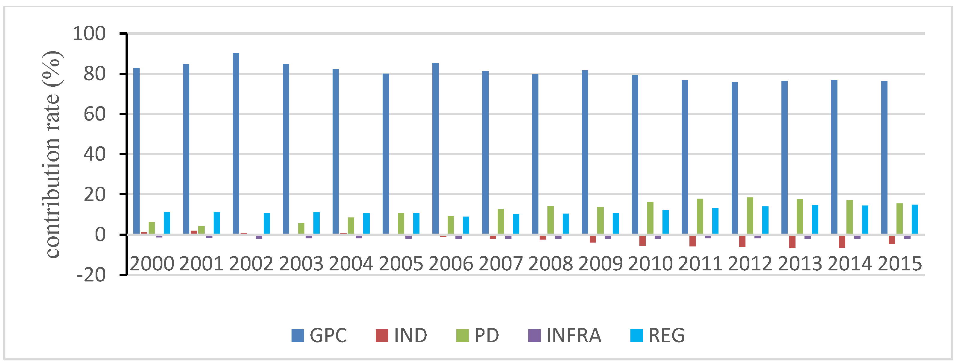
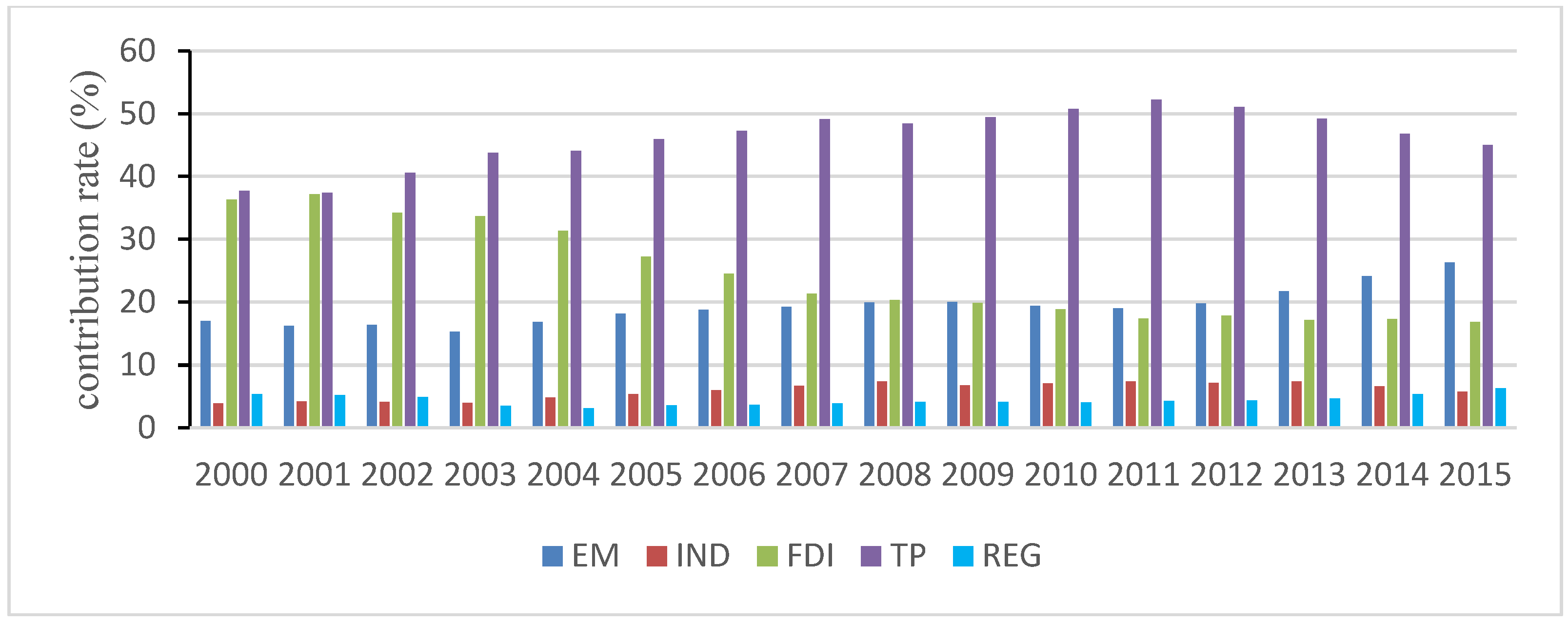
6.2. Contributions of Determinants to EPD and EID by Shapley Decomposition

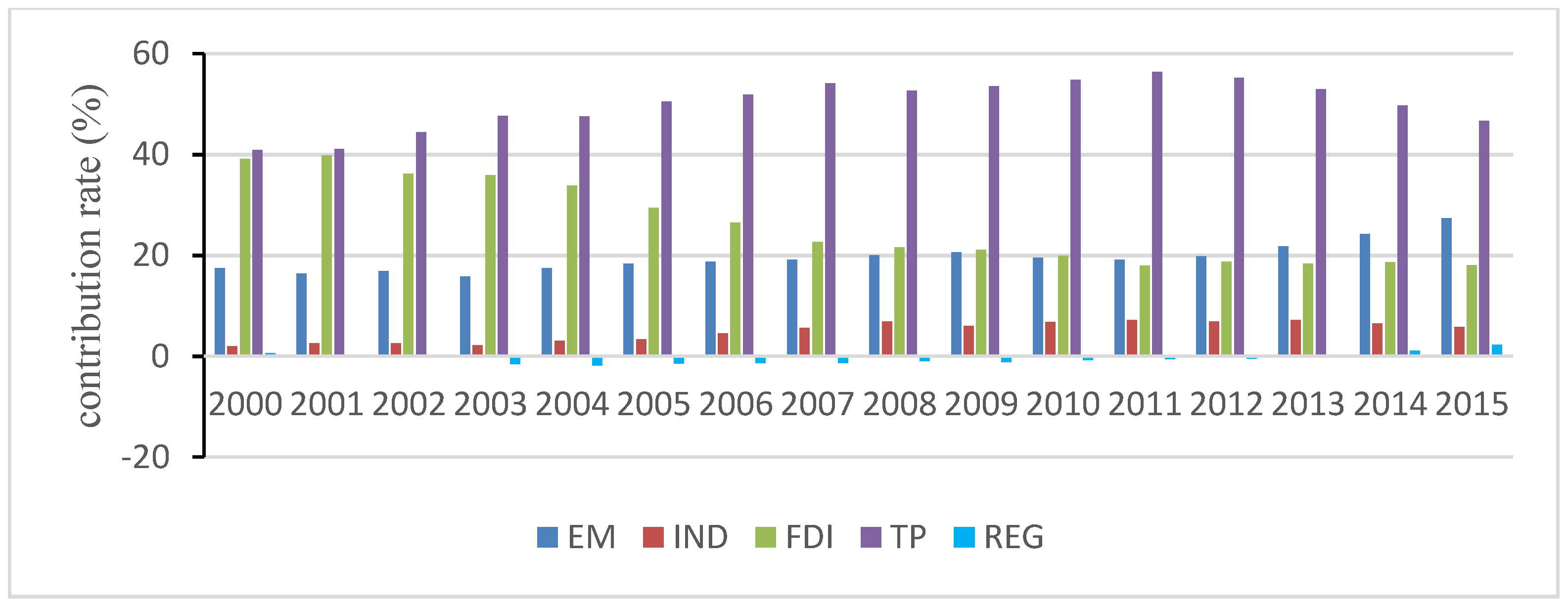
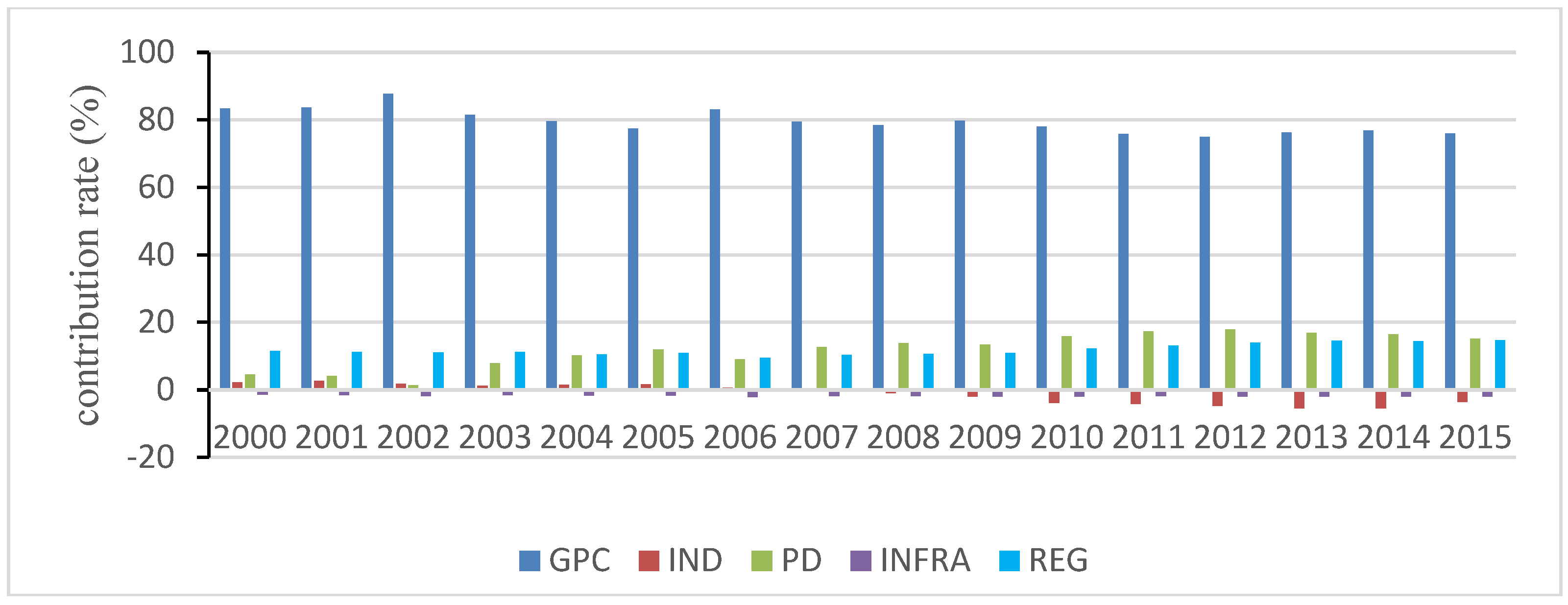
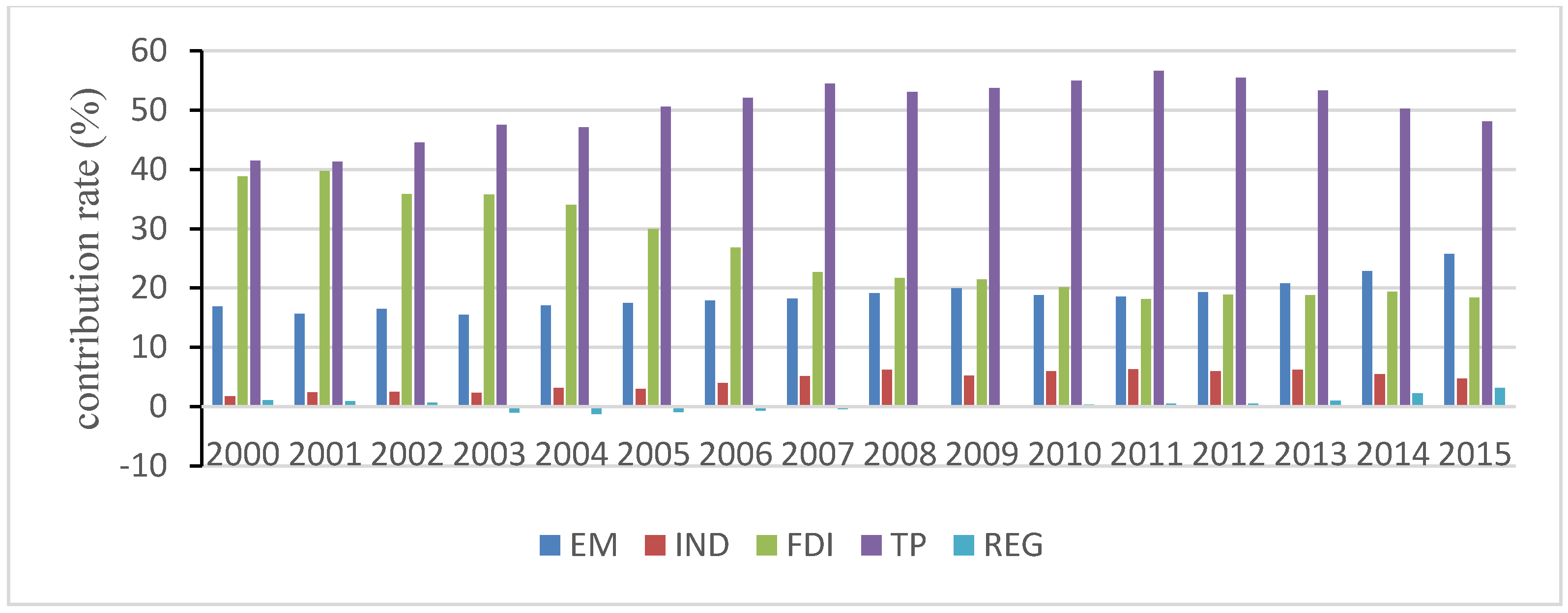
Figure 6, Figure 7 and Figure 8 show the contributions of individual determinants to EPD by using Gini, GE1 and GE0 as inequality measures, respectively. Figure 9, Figure 10 and Figure 11 present the contributions of individual determinants to EID by using Gini, GE1 and GE0 as inequality measures, respectively. In terms of the absolute value of the contribution rate, although the decomposition results differ from each other, the applications of different inequality indices will not affect the ranking of the contribution rate of each determinant to EPD (EID). Therefore, applying different inequality measures will display similar policy implications and the following discussion is mainly based on the decomposition results using the Gini coefficient as inequality measure.

Figure 6 specifies that inequality in income contributes the most to EPD with annual average contribution rate of 70%, which indicates it is the inequality in income rather than other factors that mainly influences the inter-provincial inequality in EP among 30 provinces. This finding is highly consistent with Duro et al. [15]. According to the absolute income hypothesis by Keynes, income is the dominant factor in consumption. In developed areas with higher level of economic development, the energy demand for economic growth is higher and consumption capacity is larger. Moreover, in most lagged areas, there is less financial input to support energy saving technology research. All these factors contribute to the inequality in EP. Following income, the annual average contribution rate of population density is 15.8%, which suggests that differences in population density are important factor accounting for interprovincial differences in EP. It results from that population density has a negative effect on EP in high-EP regions. Population density, such as Xinjiang, Inner Mongolia and Qinghai, is much lower than that in low-EP regions, such as Henan, Anhui and Guangdong. As for the regional factors, the annual average contribution rate of regional factors is 11.7%, which cannot be ignored because its contribution rate increases gradually. With the annual average contribution rate of 2.4%, differences in industrial structure present the smallest contribution to EPD, which indicates the impact of industrial structure is limited. In particular, although the improvement of transportation infrastructure contributes to reducing EP according to the results in Table 4, the inequality in transportation infrastructure makes little contribution to EPD because the absolute value of its annual average contribution rate to EPD is merely 0.3%.

Figure 9 indicates that EID is mainly due to differences in technological progress. The annual average contribution rate of technological progress is up to 46% and the ranking of its contribution rate is the highest during 2000–2015 with the maximal value of 52.2% in 2011. In fact, technological level in developed areas with lower EI is usually higher than that in lagged areas with higher EI. Hence, the differences in EI between high-EI regions and low-EP regions (i.e., EID) are generated. The second largest contributor to EID is the inequality in FDI, with the annual average contribution rate of 24.4%. That’s to say, differences in FDI are important factor in explaining EID. This is because EI and FDI display opposite regional differences among the Eastern, Central and Western China, that is to say, FDI in the high-EI provinces, such as Xinjiang, Inner Mongolia and Qinghai, is much less than that in Central and Eastern China with lower level of EI, such as Hubei, Beijing and Shanghai. Furthermore, according to the results of quantile regression in Table 5, FDI is conducive to reducing EI, specially, the negative effect is higher in low-EI areas. As a result, the gaps of EI between high-EI regions and low-EI regions (i.e., EID) have been yielded. Following FDI, the annual average contribution rate of energy mix is 19.2%, which suggests differences in energy mix play an important in accounting for EID. This is because energy mix has a positive effect on EI and its effect is larger in high-EI regions (see Table 5); what’s more, high-EI areas depend more on coal consumption than low-EI areas. As for industrial structure, its annual average contribution rate is 5.8%. By contrast, the inequality in regional factors has the smallest contribution to EID with annual average contribution rate of 4.3%, which indicates the impact of regional factors is limited.

According to the results of Shapley decomposition, it is found that differences in income and technological progress are main reasons for EPD and EID, respectively, which suggests convergence in both income and technological progress is of great importance to the reduction in EPD and EID among provinces, thereby achieving the integration of energy intensity reduction and energy consumption control. As newly proposed in 2017, the prominent social conflict in China lies in the unbalanced and inadequate development. In fact, there are considerable disparities in socioeconomic development among provinces, which demand our further attention to resolve.

6.3. Exploring Provincial Energy-Saving Development Path in China

In the previous discussion, quantile regression results provide important information about the changes in the impacts of all determinants on EP (EI) in provinces with different levels of EP (EI). Through the Shapley value decomposition, we find the main reasons for EPD and EID.

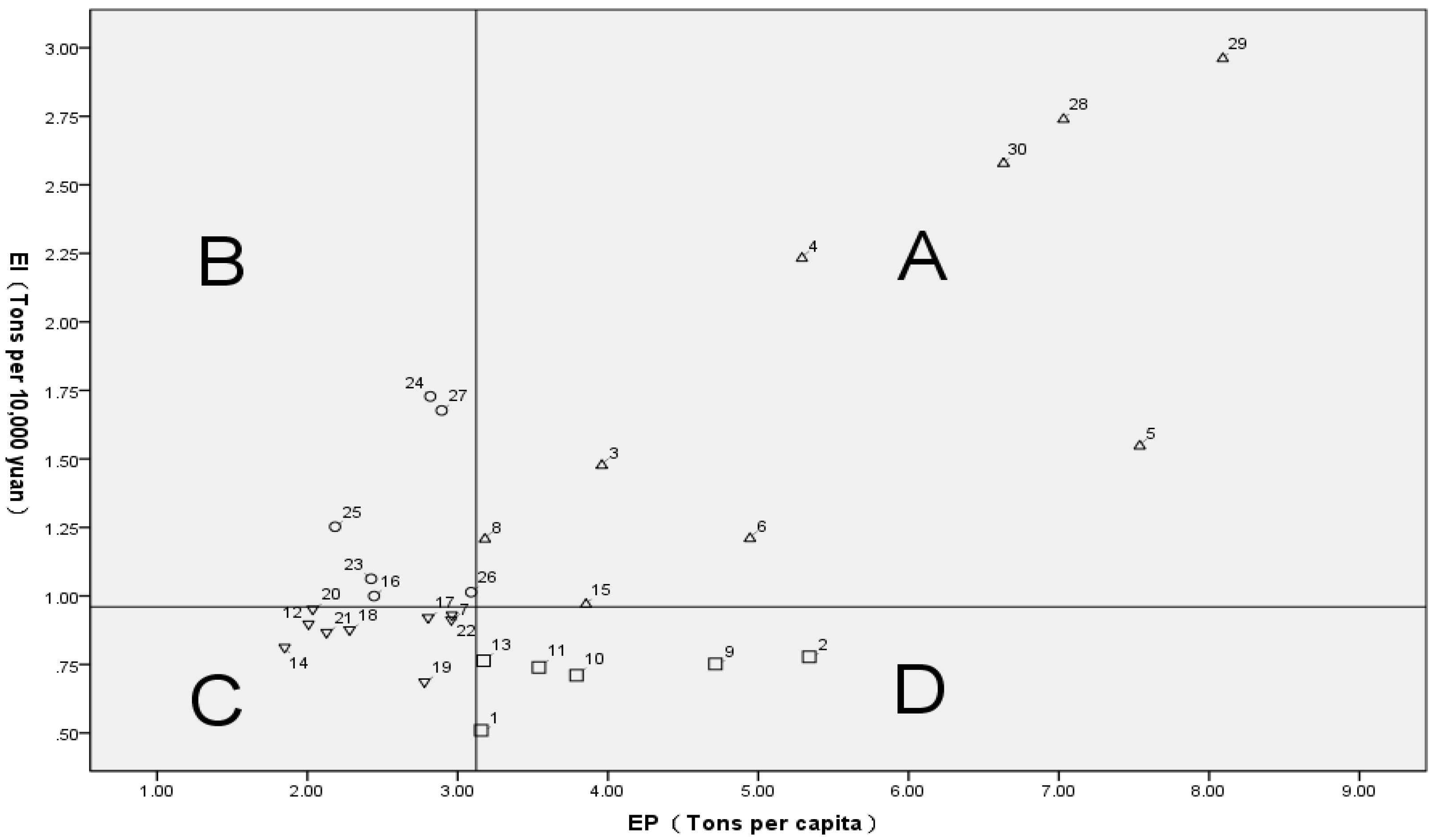
Based on the raw data of EP and EI in China’s 30 provinces during 2000–2015, the values of EP and EI at the 50% quantile are given as 2.433 and 1.466, respectively. Figure 12 is the scatter plot of provincial EP and EI in 2015, the values of EP and EI at the 50% quantile are selected as reference lines. Accordingly, 30 provinces are divided into four categories, that is, Area A with higher EP and higher EI, Area B with lower EP and higher EI, Area C with lower EP and lower EI and Area D with higher EP and lower EI. Each province’s EP and EI relative to the corresponding values at the 50% quantile are presented, which provides important information about each province’s energy-saving development pattern.

Region A includes nine provinces comprising Hebei, Shanxi, Inner Mongolia, Liaoning, Heilongjiang, Shandong, Qinghai, Ningxia and Xinjiang, most of which are rich in energy resources. It can be found that these provinces are in the extensive economic growth mainly depending on energy-intensive industries and they are in the stage of rapid developments of industrialization and urbanization. For these provinces, the choice and combination of policies are particularly important to achieve collaborative energy intensity reduction and energy consumption control. It is of great importance for these resource-based provinces to avoid the traditional extensive economic growth pattern. Specifically, it is imperative to accelerate the transformation and upgrading of industrial structure, for one thing, it is necessary to formulate measures to attract more FDI and receive the industry transferring from eastern coastal areas at the same time, thereby increasing the technology level; for another, these provinces should promote the development of high value-added and low energy-consuming industries. In addition, the high level of EI is largely due to the overwhelming coal consumption, thus, these provinces should decrease the proportion of coal consumption. Specially, this type of provinces is mainly located in northern China, these provinces should follow the way of compact development and try to enhance population agglomeration, thereby increasing the heating efficiency and avoiding resource waste.

Area B covers six provinces, that is, Henan, Sichuan, Guizhou, Yunnan, Shaanxi and Gansu. This type of provinces is mainly located in Western China. In these provinces, the flow of technology and knowledge is slow and resources are relatively deficient for their economies. According to the results of Shapley decomposition, the gap of technological progress is the main reason for EID. For these central and western provinces, the most important thing is that the government should formulate preferential policies to promote the improvement of technological level. Specifically, it is urgent to introduce advanced technology from outside and stimulate enterprises to improve the production efficiency and develop energy-saving technologies. Furthermore, it is necessary to attract more FDI capital, thereby taking advantage of the technology spillover effect. It is found that these provinces are largely dependent on coal consumption, therefore, it is expected to develop clean energy as an alternative to coal consumption, such as natural gas, solar energy and wind energy.

Region C contains nine provinces, including Jilin, Anhui, Jiangxi, Hubei, Hunan, Guangdong, Guangxi, Hainan and Chongqing. These provinces have achieved the optimal allocation and utilization of energy resources. As different provinces present distinct spatial heterogeneity in terms of EP and EI, this type of provinces should give full play to their own advantages and accelerate the pace of regional development.

Region D comprises Beijing, Tianjin, Shanghai, Jiangsu, Zhejiang and Fujian, these provinces are concentrated in eastern coastal areas and economically developed. The levels of economic development and living standard are high in these provinces, accordingly, energy demand is high as well. Although energy utilization efficiency in these provinces is quite high, EP is large as well, which confirms that the increase in energy efficiency may lead to increasing energy consumption [8,9]. Based on the results of Shapley decomposition, differences in EP among provinces are mainly attributable to differences in income. Therefore, for one thing, as these provinces belong to the group of developed areas, this type of provinces should devote sufficient resource and capital to developing energy saving technologies; for another, people tend to buy high-energy consumption products with income increasing, these provinces should actively advocate low-carbon lifestyles and enhance people’s awareness of energy conservation, such as shared bikes and electric car. Furthermore, these provinces should accelerate energy-intensive industries transferring to the central and western provinces, industry transferring not only helps relieve the resource pressure in these provinces but also contributes to improving the technological level in high-EI areas. Furthermore, these provinces are populous regions, this type of provinces should take advantage of population agglomeration in intensive utilization of resources, such as central heating, public transportation and communal facilities, thereby reducing energy consumption.

7. Conclusions and Policy Implications

This paper analyzes the inter-provincial differences in China’s energy consumption from the perspectives of energy consumption per capita (EP) and energy intensity (EI). Using the panel dataset of 30 provinces over the period 2000–2015, the quantile regression method is performed to provide evidence with regard to the issue how several influencing factors affect EP (EI), specially, the dynamic varying process of their elastic coefficients at different quantiles is also presented. The results show that the elastic coefficient of each determinant differs distinctly at different quantiles, which indicates that each factor has different effects on EP (EI) with EP (EI) increasing. According to the empirical results, income has a positive impact on EP, conversely, industrial structure, population density and transportation infrastructure play important roles in reducing EP. Furthermore, industrial structure, FDI and technological progress have negative effects on EI, while energy mix has a positive effect on EI.

The Shapley value decomposition is utilized to quantity the contributions of individual determinants to EPD and EID. The result specifies that EPD is mainly attributable to inter-provincial inequality of income and its annual average contribution rate amounts to 70%, which means differences in income level account for almost 70% of EPD. In addition, differences in population density play an important role in explaining EPD, while the inequality of transportation infrastructure contributes little to EPD. By contrast, EID is mainly due to differences in technological progress with annual average contribution rate of 46%. Following technological progress, the inequalities of FDI and energy mix are also important factors accounting for EID, with annual average contribution rates of 24.4% and 19.2%, respectively. As a whole, the contributions of industrial structure and regional factors are both small. Lastly, by the comparison of provincial EP and EI in 2015, this study explores provincial energy conservation development path, accordingly, four groups of provinces are provided with different energy-saving patterns.

The unbalanced nature of regional development across China indicates that the capacity to meet the energy conversation goal differs distinctly among regions. Based on the aforementioned conclusions, this study provides the following policy implications.

Firstly, since inequality in income is the most important factor in explaining differences in EP, it is of great significance to promote the coordinated development of regional economy. Our findings show that income has a positive effect on EP, while a negative effect on energy intensity. For some provinces with rich energy resources, high energy-saving potential and lagged economic development, such as Ningxia, Qinghai and Inner Mongolia, financial assistance should be enhanced to support technology research so as to improve energy utilization efficiency and reduce energy consumption. In addition, in the course of rapid economic development, people’s income levels and living standards are improved, so does the level of energy consumption. Thus, it is supposed to enhance people’s energy-saving awareness and promote a low-carbon life.

Secondly, inequality in FDI plays an important role in accounting for differences in EI. Thus, it is urgent for backward areas to attract more foreign capital. For some central and western regions, the degree of openness is not high and there is poor favorable condition for foreign investment. It is particularly important to formulate relevant policies to attract more FDI inflows. Nevertheless, it is necessary to appropriately enhance the environmental regulations, thereby restricting foreign high-energy consumption companies. At the same time, local governments should encourage enterprises to follow the energy-saving development pattern

Thirdly, inequality in energy mix is an important factor in explaining differences in EI, the traditional energy consumption pattern based on large share of coal consumption is supposed to be improved, especially for some high-EI areas, such as Shanxi, Hebei and Liaoning. The development of clean energy, such as natural gas, hydropower, solar energy and wind energy, is not only the inevitable choice of environmental protection but also an effective measure for energy conservation and consumption reduction. In addition, given China’s resource endowment, it is imperative to improve the utilization efficiency of coal at the technical level in the long term.

Fourthly, although differences in industrial structure contribute little to EPD and EID, economic restructuring is effective in decreasing both EP and EI. During the process of industrialization, it is supposed to promote the growth of technology scale. Specifically, industrial capital intensity and technology intensification are to be heightened, hence, energy consumption may present the trend of marginal decline. At the same time, with the deep development of industrialization, local governments should accelerate the transformation of industrial structure and promote the development of low-energy industries, such as service and high-tech industries. Specially, high-EI provinces are expected to receive the industry transferring from some low-EI provinces in eastern coastal areas.

Fifthly, the differences in technological progress are the most significant reason for inequality in EI and the negative effect of technological progress on EI is larger in high-EI areas. Therefore, it is urgent to improve the technological level in high-EI areas mainly located in Central and Western China, so as to narrow technological gap among regions. Specifically, on the one hand, it is advisable for high-EI areas to promote the collaborative innovation of Industry-University-Research, which breaks barriers between multiple subjects, emphasizes resources sharing and becomes an important way of independent innovation; on the other hand, it is necessary to promote technology diffusion by learning and introducing energy saving technology.

Sixthly, the effect of population density on EP cannot be ignored. It is indispensable to promote compact development and enhance population agglomeration in both urban and rural areas. Population agglomeration is beneficial to energy intensive utilization, thereby enhancing the “density effect” and concealing the “scale effect”. Specifically, on the one hand, compact development contributes to promoting public transportation and reducing traffic energy consumption; on the other hand, it helps improve heating efficiency and avoid resource waste.

Last but not least, inequality in persistent regional factors cannot be ignored in policy making. For some provinces with abundant energy resources and high proportion of coal consumption, such as Qinghai, Xinjiang and Shanxi, there is a need to introduce advanced production capacity from developed regions so as to maximize the benefits of energy resource utilization. Meanwhile, the allocation and structure of resources are to be optimized among provinces, an integrated energy market can be formed [63], thereby reducing the gap of energy supply and demand among provinces.

References

1. Li, Y.; Sun, L.Y.; Feng, T.W.; Zhu, C.Y. How to reduce energy intensity in China: A regional comparison perspective. Energy Policy 2013, 61, 513–522. [Google Scholar] [CrossRef]
2. Zhang, L.; Yu, J.; Sovacool, B.K.; Ren, J. Measuring energy security performance within China: Toward an inter-provincial prospective. Energy 2017, 125, 825–836. [Google Scholar] [CrossRef]
3. British Petroleum. BP Statistical Review of World Energy; British Petroleum: London, UK, 2017. [Google Scholar]
4. British Petroleum. BP Energy Outlook 2035, 2017 ed.; British Petroleum: London, UK, 2017. [Google Scholar]
5. Dong, F.; Li, X.; Long, R.; Liu, X. Regional carbon emission performance in China according to a stochastic frontier model. Renew. Sustain. Energy Rev. 2013, 28, 525–530. [Google Scholar] [CrossRef]
6. Dong, F.; Yu, B.L.; Hadachin, T.; Dai, Y.J.; Wang, Y.; Zhang, S.N.; Long, R.Y. Drivers of carbon emission intensity change in China. Resour. Conserv. Recycl. 2018, 129, 187–201. [Google Scholar] [CrossRef]
7. Liddle, B. Electricity intensity convergence in IEA/OECD countries: Aggregate and sectoral analysis. Energy Policy 2009, 37, 1470–1478. [Google Scholar] [CrossRef]
8. Greening, L.A.; Greene, D.L.; Difiglio, C. Energy efficiency and consumption-the rebound effect-a survey. Energy Policy 2000, 28, 389–401. [Google Scholar] [CrossRef]
9. Gillingham, K.; Rapson, D.; Wagner, G. The rebound effect and energy efficiency policy. Rev. Environ. Econ. Policy 2016, 10, 68–88. [Google Scholar] [CrossRef]
10. Markandya, A.; Pedroso-Galinato, S.; Streimikiene, D. Energy intensity in transition economies: Is there convergence towards the EU average? Energy Econ. 2006, 28, 121–145. [Google Scholar] [CrossRef]
11. Xiong, S.; Tian, Y.; Ji, J.; Ma, X. Allocation of energy consumption among provinces in China: A Weighted ZSG-DEA Model. Sustainability 2017, 9, 2115. [Google Scholar] [CrossRef]
12. Duro, J.A.; Padilla, E. International inequalities in per capita CO2 emissions: A decomposition methodology by Kaya factors. Energy Econ. 2006, 28, 170–187. [Google Scholar] [CrossRef]
13. Alcantara, V.; Duro, J.A. Inequality of energy intensities across OECD countries: A note. Energy Policy 2004, 32, 1257–1260. [Google Scholar] [CrossRef]
14. Duro, J.A.; Padilla, E. Inequality across countries in energy intensities: An analysis of the role of energy transformation and final energy consumption. Energy Econ. 2011, 33, 474–479. [Google Scholar] [CrossRef]
15. Duro, J.A.; Alcántara, V.; Padill, E. International inequality in energy intensity levels and the role of production composition and energy efficiency: An analysis of OECD countries. Ecol. Econ. 2010, 69, 2468–2474. [Google Scholar] [CrossRef]
16. Duro, J.A.; Teixido-Figueras, J.J. Ecological footprint inequality across countries: The role of environment intensity, income and interaction effects. Ecol. Econ. 2013, 93, 34–41. [Google Scholar] [CrossRef]
17. White, T.J. Sharing resources: The global distribution of the ecological footprint. Ecol. Econ. 2007, 64, 402–410. [Google Scholar] [CrossRef]
18. Teixido-Figueras, J.; Duro, J.A. The building blocks of International Ecological Footprint inequality: A Regression-Based Decomposition. Ecol. Econ. 2015, 118, 30–39. [Google Scholar] [CrossRef]
19. Clarke-Sather, A.; Qu, J.; Wang, Q.; Zeng, J.; Li, Y. Carbon inequality at the subnational scale: A case study of provincial-level inequality in CO2 emissions in China 1997–2007. Energy Policy 2011, 39, 5420–5428. [Google Scholar] [CrossRef]
20. Burnett, J.W.; Madariaga, J. The convergence of U.S. state-level energy intensity. Energy Econ. 2016, 62, 357–370. [Google Scholar] [CrossRef]
21. Ezcurra, R. Distribution dynamics of energy intensities: A cross-country analysis. Energy Policy 2007, 35, 5254–5259. [Google Scholar] [CrossRef]
22. Liddle, B. Revisiting world energy intensity convergence for regional differences. Appl. Energy 2010, 87, 3218–3225. [Google Scholar] [CrossRef]
23. Mielnik, O.; Goldemberg, J. Converging to a common pattern of energy use in developing and industrialized countries. Energy Policy 2000, 28, 503–508. [Google Scholar] [CrossRef]
24. Nielsson, L. Energy intensity in 31 industrial and developing countries 1950–1988. Energy 1993, 18, 309–322. [Google Scholar] [CrossRef]
25. Herrerias, M.J. World energy intensity convergence revisited: A weighted distribution dynamics approach. Energy Policy 2012, 49, 383–399. [Google Scholar] [CrossRef]
26. Dong, F.; Long, R.; Yu, B.; Wang, Y.; Li, J.; Wang, Y.; Dai, Y.; Yang, Q.; Chen, H. How can China allocate CO2 reduction targets at the provincial level considering both equity and efficiency? Evidence from its Copenhagen Accord pledge. Resour. Conserv. Recycl. 2018, 130, 31–43. [Google Scholar] [CrossRef]
27. Dong, F.; Long, R.; Li, Z.; Dai, Y. Analysis of carbon emission intensity, urbanization and energy mix: Evidence from China. Nat. Hazards 2016, 82, 1375–1391. [Google Scholar] [CrossRef]
28. Jiang, X.M.; Duan, Y.W.; Green, C. Regional disparity in energy intensity of China and the role of industrial and export structure. Resour. Conserv. Recycl. 2017, 120, 209–218. [Google Scholar] [CrossRef]
29. Yang, J.; Wang, J.; Zhang, Z.Y. Inter-provincial discrepancy and abatement target achievement in carbon emissions: A study on carbon Lorenz curve. Acta Sci. Circumstantiae 2012, 32, 2016–2023. [Google Scholar]
30. Chen, J.; Cheng, S.; Song, M. Decomposing inequality in energy-related CO2 emissions by source and source increment: The roles of production and residential consumption. Energy Policy 2017, 107, 698–710. [Google Scholar] [CrossRef]
31. Padilla, E.; Serrano, A. Inequality in CO2 emissions across countries and its relationship with income inequality: A distributive approach. Energy Policy 2006, 34, 1762–1772. [Google Scholar] [CrossRef]
32. Koenker, R.; Bassett, G. Regression Quantile. Econometrica 1978, 46, 33–50. [Google Scholar] [CrossRef]
33. Chay, K.Y.; Honore, B.E. Estimation of semiparametric censored regression models: An application to changes in black-white earnings inequality during the 1960s. J. Hum. Resour. 1998, 33, 4–38. [Google Scholar] [CrossRef]
34. Melly, B. Decomposition of differences in distribution using quantile regression. Labour Econ. 2005, 12, 577–590. [Google Scholar] [CrossRef]
35. Bedi, A.; Edwards, J. The impact of school quality on earnings and educational returns—Evidence from a low-income country. J. Dev. Econ. 2002, 68, 157–185. [Google Scholar] [CrossRef]
36. Abrevaya, J. The effects of demographics and maternal behavior on the distribution of birth outcomes. In Economic Applications of Quantile Regression; Springer: Berlin/Heidelberg, Germany, 2002; pp. 247–257. [Google Scholar]
37. Fields, G.S.; Yoo, G. Falling labor income inequality in Korea. Rev. Income 2000, 46, 139–159. [Google Scholar] [CrossRef]
38. Morduch, J.; Sicular, T. Rethinking inequality decomposition, with evidence from rural China. Econ. J. 2002, 112, 93–106. [Google Scholar] [CrossRef]
39. Shorrocks, A.F. Decomposition procedures for distributional analysis: A unified framework based on the Shapley value. J. Econ. Inequal. 1999, 11, 99–126. [Google Scholar] [CrossRef]
40. Wan, G. Regression-Based Inequality Decomposition: Pitfalls and a Solution Procedur; WIDER Discussion Papers//World Institute for Development Economics (UNU-WIDER); United Nations University World Institute for Development Economics Research: Helsinki, Finland, 2002. [Google Scholar]
41. Wan, G. Accounting for income inequality in rural China: A regression-based approach. J. Comp. Econ. 2004, 32, 348–363. [Google Scholar] [CrossRef]
42. Han, L.Y.; Xu, X.K.; Han, L. Applying quantile regression and Shapley decomposition to analyzing the determinants of household embedded carbon emissions: Evidence from urban China. J. Clean. Prod. 2015, 103, 219–230. [Google Scholar] [CrossRef]
43. Xu, X.K.; Han, L.Y.; Lv, X.F. Household carbon inequality in urban China, its sources and determinants. Ecol. Econ. 2016, 128, 77–86. [Google Scholar] [CrossRef]
44. Shorrocks, A.F. inequality decomposition by factor components. Econometrica 1982, 50, 193–212. [Google Scholar] [CrossRef]
45. Cai, Z.X. Density effects, development level and China’s urban carbon dioxide emission. Econ. Probl. 2013, 3, 25–31. (In Chinese) [Google Scholar]
46. Zheng, Y.; Qi, J.; Chen, X. The effect of increasing exports on industrial energy intensity in China. Energy Policy 2011, 39, 2688–2698. [Google Scholar] [CrossRef]
47. Henderson, V. The urbanization process and economic growth: The so-what question. J. Econ. Growth 2003, 8, 47–71. [Google Scholar] [CrossRef]
48. Liddle, B.; Messinis, G. Which comes first-urbanization or economic growth? Evidence from heterogeneous panel causality tests. Appl. Econ. Lett. 2015, 22, 349–355. [Google Scholar] [CrossRef]
49. Liddle, B. Consumption-driven environmental impact and age structure change in OECD countries: A cointegration-STIRPAT analysis. Demogr. Res. 2011, 24, 749–770. [Google Scholar] [CrossRef]
50. Liddle, B.; Lung, S. Might electricity consumption cause urbanization instead? Evidence from heterogeneous panel long-run causality tests. Glob. Environ. Chang. 2014, 24, 42–51. [Google Scholar] [CrossRef] [Green Version]
51. Zhang, A.; Wang, R. Research on the dynamic relationship between energy consumption, economic growth and international trade in different regions of China. East China Econ. Manag. 2016, 30, 68–74. (In Chinese) [Google Scholar]
52. Wan, G.; Zhou, Z. Income inequality in rural China: Regression-based decomposition using household data. Rev. Dev. Econ. 2005, 9, 107–120. [Google Scholar] [CrossRef]
53. National Bureau of Statistics of China. China Statistical Yearbook; China Statistics Press: Beijing, China, 2016. (In Chinese)
54. National Bureau of Statistics of China. China Energy Statistical Yearbook; China Statistics Press: Beijing, China, 2016. (In Chinese)
55. National Bureau of Statistics of China. China City Statistical Yearbook; China Statistics Press: Beijing, China, 2016. (In Chinese)
56. Rogers, W.H. Quantile regression standard errors. Stata Tech. Bull. 1993, 9, 16–19. [Google Scholar]
57. Chen, Q. Advanced Econometrics and Stata Applications, 2nd ed.; Higher Education Press: Beijing, China, 2014. (In Chinese) [Google Scholar]
58. Herrerias, M.J.; Cuadros, A.; Luo, D. Foreign versus indigenous innovation and energy intensity: Further research across Chinese regions. Appl. Energy 2016, 162, 1374–1384. [Google Scholar] [CrossRef]
59. Li, J.; Ran, G.; Wan, G. Study on the disparities of regional financial development in China: Based on the theory of division of labor and decomposition method of Shapley value. Econ. Res. J. 2007, 5, 42–55. (In Chinese) [Google Scholar]
60. Wan, G.; Lu, M.; Chen, Z. Globalization and regional inequality: Chinese evidence. Soc. Sci. China 2005, 3, 17–26. (In Chinese) [Google Scholar]
61. Otsuka, A. Population agglomeration and residential energy consumption: Evidence from Japan. Sustainability 2018, 10, 469. [Google Scholar] [CrossRef]
62. Huang, J.B.; Du, D.; Tao, Q.Z. An analysis of technological factors and energy intensity in China. Energy Policy 2017, 109, 1–9. [Google Scholar] [CrossRef]
63. Sheng, Y.; Shi, X.P.; Zhang, D. Economic growth, regional disparities and energy demand in China. Energy Policy 2014, 71, 31–39. [Google Scholar] [CrossRef]
Figure 1. Framework of this research.
Sustainability 10 01806 g001
Figure 2. Regional distribution of energy consumption per capita (EP) in China in 2015 (Tons per capita).
Sustainability 10 01806 g002
Figure 3. Regional distribution of energy intensity (EI) in China in 2015 (Tons per 10,000 yuan).
Sustainability 10 01806 g003
Figure 4. EPD of China’s 30 provinces in 2000–2015 estimated by three indicators.
Sustainability 10 01806 g004
Figure 5. EID of China’s 30 provinces in 2000–2015 estimated by three indicators.
Sustainability 10 01806 g005
Figure 6. Decomposition result of EPD measured by Gini coefficient.
Sustainability 10 01806 g006
Figure 7. Decomposition result of EPD measured by GE1.
Sustainability 10 01806 g007
Figure 8. Decomposition result of EPD measured by GE0.
Sustainability 10 01806 g008
Figure 9. Decomposition result of EID measured by Gini coefficient.
Sustainability 10 01806 g009
Figure 10. Decomposition result of EID measured by GE1.
Sustainability 10 01806 g010
Figure 11. Decomposition result of EID measured by GE0.
Sustainability 10 01806 g011
Figure 12. Comparison of provincial EP and EI in 2015. Note: Numbers 1–30 represent 30 provinces in China shown in Table A1.
Sustainability 10 01806 g012