Daily Monitoring of Shallow and Fine-Grained Water Patterns in Wet Grasslands Combining Aerial LiDAR Data and In Situ Piezometric Measurements

Abstract

The real-time monitoring of hydrodynamics in wetlands at fine spatial and temporal scales is crucial for understanding ecological and hydrological processes. The key interest of light detection and ranging (LiDAR) data is its ability to accurately detect microtopography. However, how such data may account for subtle wetland flooding changes in both space and time still needs to be tested, even though the degree to which these changes impact biodiversity patterns is of upmost importance. This study assesses the use of 1 m × 1 m resolution aerial LiDAR data in combination with in situ piezometric measurements in order to predict the flooded areas at a daily scale along a one-year hydrological period. The simulation was applied over 663 ha of wet grasslands distributed on six sites across the Marais Poitevin (France). A set of seven remote sensing images was used as the reference data in order to validate the simulation and provide a high overall accuracy (76–94%). The best results were observed in areas where the ditch density was low, whereas the highly drained sites showed a discrepancy with the predicted flooded areas. The landscape proportion index was calculated for the daily steps. The results highlighted the spatiotemporal dynamics of the shallow flooded areas. We showed that the differences in the flooding durations among the years were mainly related to a narrow contrast in topography (40 cm), and occurred over a short period of time (two months).

1. Introduction

In wetlands, hydrological processes affect biogeochemical and ecological functions together with hydrological hazards [1]. As an example, runoff from rivers to wetlands prevent flood risks in downstream urbanized areas [2]; hydrological pulses transport phosphorus into the floodplain drainage network [3]; the flood duration drives plant diversity and functional traits in wet grasslands [4]; and the water level in grasslands affects bird diversity [5]. However, the flooding pattern and its dynamics along space and time are still poorly understood, and as a consequence they are also poorly predicted [6]. Some of the main challenges include producing: (1) reliable predictions while taking the subtle spatial heterogeneity of marshlands into account, and (2) predictions that may fit the large variations that are observed for the flooding areas over a short period of time. In order to address these challenges, data with both spatial fine-scale and intensive temporal resolutions for the flooding proxies are required.

There have been recent advances in Earth observation technology, including improved spatial, temporal, spectral, and radiometric resolutions [7]; however, the monitoring of shallow and fine-grained water pattern dynamics is still limited by the trade-off between either high-resolution images or images with intensive repetition over time [8]. As an example, some studies have shown an interest in SAR (Synthetic Aperture Radar) time series for monitoring flooded areas in wetlands at a regional scale [9,10], while other studies have underlined an interest in single-date light detection and ranging (LiDAR) intensity [11] or multispectral data [12] for detecting fine-scale spatial patterns in the flooding of shallow waters.

Earth observation data can be used to calibrate and develop flood models [13]. Topographic data are crucial for hydraulic modeling, particularly in wetlands where the topography affects water runoff [1]. Topographic data are also the most significant source of uncertainty [14]; consequently, the broad digital elevation model (DEM) derived from SAR data such as SRTM (Shuttle Radar Topography Mission), or, more recently, TanDEM-X (TerraSAR-X add-on for Digital Elevation Measurement) are only appropriate for large-scale flood studies [8]. Conversely, LiDAR-based digital terrain models (DTM) provide high-resolution spatial information, and have been found to be suitable for the characterization of subtle ground altimetry variations in wetlands [15]. As a result, many studies have pointed out the strong influence of microtopography that has been derived from LiDAR DTMs and shallow patterns in overland flow simulations [16,17,18,19,20,21]. As an example, a LiDAR-based DTM was used to successfully assess the maximum water storage capacity in wetlands [22], model a storm event at the watershed scale [23], and simulate the discontinuous puddle-to-puddle overland flow dynamics for infiltrating surfaces [24]. However, the modeling of the spatiotemporal dynamics of floods at a daily step remains a challenging task [24]. Although LiDAR-based DTMs have been used to characterize the overflow-driven lateral connectivity between streams and floodplains [25,26,27,28], the results showed a severe underestimation of flood events due to the subtle connectivity between wetlands and streams. Floodplains are often connected through small intermittent creeks, which were not captured by the LiDAR data [25]. Similarly, runoff models based on LiDAR and climatic datasets [29] were not accurate enough in wetlands with agricultural activities, as the ditch network cuts off the runoff of water, and prevents classical drainage models from correctly representing the flow paths [30].

Alternatively, Maclean et al. [31] modeled the soil and water surface conditions at the fine scale and for the daily steps using a 1 m × 1 m resolution LiDAR-based DTM, climatic measurements, vegetation maps, and soil maps. This approach is certainly relevant for monitoring shallow and fine-grained water patterns, but its major limitation lies in the uncertainty in the water budget, as it is indirectly assessed using climatic (e.g., precipitation, solar radiation), soil (e.g., infiltration), and topographic variables (e.g., runoff). Additional uncertainties were introduced by the model parameters (e.g., arbitrary constant values), input data (e.g., broad vegetation and soil maps), or water-retention mechanism [8].

For several decades now, hourly fluctuations in the groundwater level can be directly measured using a piezometric probe system. When located in wetlands rather than in rivers, these piezometric probes provide a direct measure of the water table, and thus provide real and accurate data for the modeling of the water budget. Incidentally, the quality of such a piezometric time series was shown to be suitable for evaluating the effect of wetland flooding on biodiversity and biogeochemistry [4]. However, such information is only available in very few places, and it is still unknown whether or not they may be generalized over whole wetland areas.

This work addresses the challenge of characterizing the flood patterns in wetlands with sufficient accuracy in both space and time with respect to the ecological processes and biota. With this in mind, we combine high spatial resolution LiDAR data with high temporal resolution in situ piezometric probe measurements in order to model daily flood maps over a 663-ha wetland area. This model also provides the basis for monitoring the spatiotemporal dynamics of floods in wet grasslands. The advances as well as the limitations of this model for the understanding of ecohydrology processes are discussed.

2. Materials and Methods

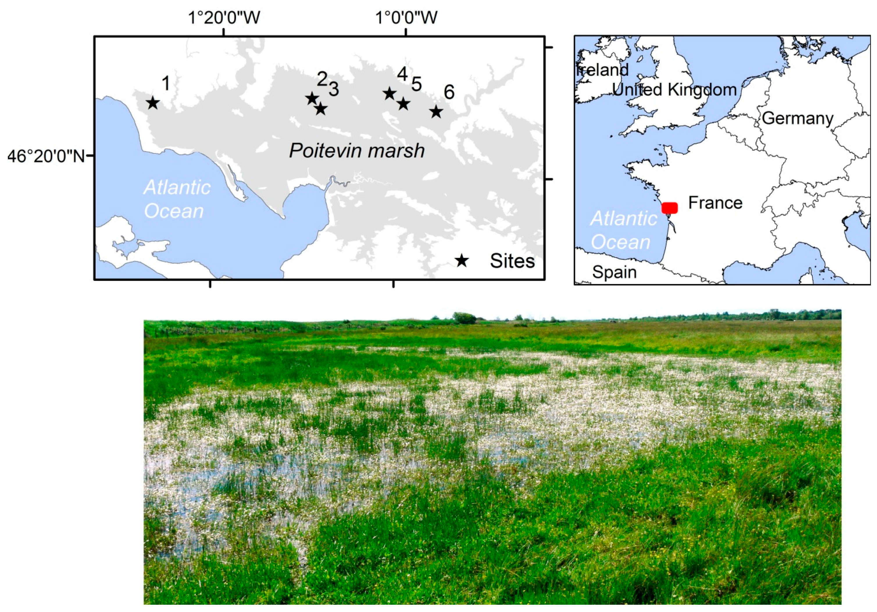
2.1. Study Area

The study area comprises six sites for a total of 663 hectares of wet grassland distributed across the Marais Poitevin, a marshland area near the French Atlantic coast (46.4°N, 1.2°W) (Figure 1). The climate is oceanic temperate, with a mean monthly minimum/maximum temperature ranging from 2/10 °C in winter to 12/24 °C in summer. The mean annual precipitation ranges from 700 mm to 900 mm, with a summer water deficit. Deriving from salt marshes after embankment, the studied marshland shows an elevation gradient of limited extent, with depressions that are 50–80 cm deep, and upper flats. The elevation ranges between 1.4–3.1 m above sea level. A high-density ditch network efficiently drained the marsh for agriculture activities (

Table 1. Characteristics of the sites.

Site	Area (ha)	Min–Max Altimetry (meters)	Ditch Density (meters/ha)	Land Owner	Flood Retention
1	215	1.4–2.6	87	Private	Yes
2	68	1.8–2.9	163	Private	No
3	103	1.2–2.3	114	Private	Yes
4	95	1.9–2.7	79	Municipal	Yes
5	15	1.9–3.0	233	Private	No
6	167	2.1–3.1	54	Municipal	Yes

). However, the grasslands may be flooded from winter to spring, when the soils are waterlogged and there is significant precipitation. Therefore, the study area is affected with biodiversity [32], and is part of the NATURA 2000 European network [33]. As a consequence, management of the water level is subjected to a trade-off between economic and ecological issues.

2.2. Data Collection and Pre-Processing

A 1 m × 1 m resolution digital terrain model (DTM)—the Litto3D product—was delivered by the French Mapping Agency (IGN, Saint Mandé, France). It was derived from airborne LiDAR (light detection and ranging) data acquired in the summer of 2012 with a 2 pts/m² point density. In grasslands, the altimetric accuracy of the LiDAR data usually ranges from 5 cm to 30 cm, depending on the vegetation height and density cover [15]. In order to assess the altimetric accuracy of the LiDAR-based DTM, differential global positioning system (DGPS) plots (n = 395) with a 2-cm altimetry accuracy were recorded across the six sites along topographic transects. The DTM values are expressed relative to sea level in the French national georeferencing system (NGF-93). In order to reduce the raster size, the DTMs were clipped and analyzed according to the boundaries of the sites.

A piezometric probe was installed in October 2014 in the lower part of each site. The water level elevations were recorded hourly with an accuracy of 2 cm. The probe values are also expressed in NGF-93. The database for each probe was collected during the field visits (the last in March 2016), and the hourly water levels were averaged daily.

A set of seven earth observation images, including two aerial photographs and five SPOT-6/7 multispectral images, was collected in order to validate the simulated flood maps, and used as the reference data (

Table 2. Characteristics of the Earth observation images used for the validation.

Acquisition Date	Sensor	Spatial Resolution	Site Coverage
4 March 2015	Microlight aircraft	1.0 m	2, 3, 4, 5, 6
12 April 2015	SPOT-6	1.5 m	3, 4, 5, 6
8 June 2015	SPOT-6	1.5 m	1, 3
28 June 2015	SPOT-7	1.5 m	1, 2, 3
15 January 2016	Microlight aircraft	1.0 m	1
14 March 2016	SPOT-7	1.5 m	3, 4, 5, 6
20 March 2016	SPOT-6	1.5 m	2

). The two aerial images acquired by the microlight aircraft during the winter flooding periods were used as the reference data, with a first acquisition campaign on 4 March 2015 for sites 2–6, and a second campaign on 15 January 2016 for site 1. The aerial images were orthorectified and georeferenced using the spline transformation from ArcGIS (ESRI, Redlands, CA, USA). Approximately 50 to 60 reference points were chosen on each site based on cross ditches that were easily identifiable on both the aerial image and the LiDAR-based DTM. The SPOT-6/7 images were delivered free of charge from the Geosud archive catalog (ids.equipex-geosud.fr) as an orthorectified level product. A total of five cloud-free SPOT-6/7 images were found to be usable for all or part of the area of the six sites. The SPOT-6/7 sensors featured panchromatic (450–745 nm), blue (450–525 nm), green (530–590 nm), red (625–695 nm), and near-infrared (760–890 nm) spectral bands, and had a spatial resolution of 6.0 m and 1.5 m in multispectral and panchromatic mode, respectively. In order to improve the spatial resolution of the multispectral bands to 1.5 m, a pan-sharpening process was applied by Gram–Schmidt fusion [34]. Each site was covered by at least three remote sensing images.

2.3. Model Calibration and Validation

To model the flood extent at a daily step interval, the LiDAR-based DTM dataset was used and transformed into a binary raster (0 = unflooded; 1 = flooded) that was specific to each site, according to the daily water level measured by the piezometric probe. The model was iteratively performed using the R software [27] with the Raster package [28]. Since the accuracy of the LiDAR-based DTM altimetry values range between 5–30 cm in grasslands [29], a site-specific DTM calibration was necessary. For each DGPS plot, the elevation value was compared with the corresponding DTM pixel value. Within each site, the median elevation difference value measured between the DGPS plots and the DTM was assigned as the offset value. We assumed that the altimetry offset is constant across a site. Consequently, the same offset value was added to the DTM pixel value, and resulted in site-specific calibrated DTMs.

In order to validate the model, we performed a cross-validation for each site between the flooding areas, which was measured from the remote sensing reference images with the areas simulated in the LiDAR-based DTM. The flood extents observed on each remote sensing image were semi-automatically extracted by an object-based approach. Specifically, a multiresolution segmentation was applied to merge each adjacent pixel into objects with similar values [35] using the eCognition software (Definiens Imaging, Munich, Germany). As the spectral response of the flooded areas showed large variability depending on the sensor type (pan-sharpened multispectral imagery, microlight aircraft) and environmental conditions (water depth, vegetation height, wind force, etc.), the objects were manually sorted into unflooded or flooded categories. Considering that the studied sites were covered by herbaceous vegetation, we assumed that a minimum water depth of 15 cm was required in order to be detectable on the aerial image. Simulated flooded pixels with a water depth of less than 15 cm were thereafter reclassified as unflooded for the validation.

The comparison between the observed and simulated flood extents produced overall accuracy (OA) and Kappa location (K_loc) indexes. These analyses were carried out using the Idrisi GIS software (Clark labs, Worcester, MA, USA). The popular OA index provides information on the proportion of pixels that are correctly simulated. The K_loc index is a variation of the standard Kappa index of agreement, but takes the spatial location of the errors into account [36]. It was calculated according to the following Equation (1):

$$K_{loc}= \frac{Po - Pc}{Pp - Pc}$$

(1)

where Po is the observed proportion of cells that are correctly classified, Pc is the expected proportion that is correct due to chance, and Pp is the proportion that is correct when the classification is perfect.

Pc was expressed as follows in Equation (2):

$$Pc={\displaystyle \sum }_{j=1}^j\left(S_j\times R_j\right)$$

(2)

where Pc is the expected proportion that is correct due to chance, S_j is the proportion of cells in category j in the simulation, and R_j is the proportion of cells in category j in the reference.

Pp was expressed as follows in Equation (3):

$$Pp={\displaystyle \sum }_{j=1}^j\min \left(S_j,R_j\right)$$

(3)

where Pp is the proportion that is correct when the classification is perfect, S_j is the proportion of cells in category j in the simulation, and R_j is the proportion of cells in category j in the reference.

Regarding the K_loc values, we considered the simulation performances as poor when <0.4; as moderate for values between 0.41–0.60; and as good or excellent when respectively between 0.61–0.80 and >0.81.

2.4. Spatiotemporal Monitoring and Characterization of the Flood Patterns

The flood extents were modeled daily for each site during one hydrological year, from 1 November 2014 to 31 October 2015. Each daily simulated map of the flood extent was iteratively added in order to produce the annual flood duration map. Transitional maps representing the cumulative flood duration were produced at a bi-monthly interval. All of the output maps were modeled with a 1 m × 1 m resolution.

In order to quantify the temporal changes regarding the flooded area, the “landscape proportion index” (LPI) was calculated daily and for each site, from the simulated flood maps using the SDMTools R-package [32]. The landscape analysis was performed separately on both the flooded and unflooded categories. The LPI describes the proportional abundance of each patch category in each site. The LPI is calculated as follows in Equation (4):

$$LPI=\frac{{\sum }_{j=1}^n{a}_{ij }}{A}$$

(4)

where LPI is the landscape proportion index; a_ij is the area of patch ij in m²; and A is the total area in m² in each site.

In order to compare the hydrological performance between the sites, a hierarchical clustering of the LPI time series was applied using a shape-based distance [37] that was implemented in the dtwclust R-package [38].

3. Results

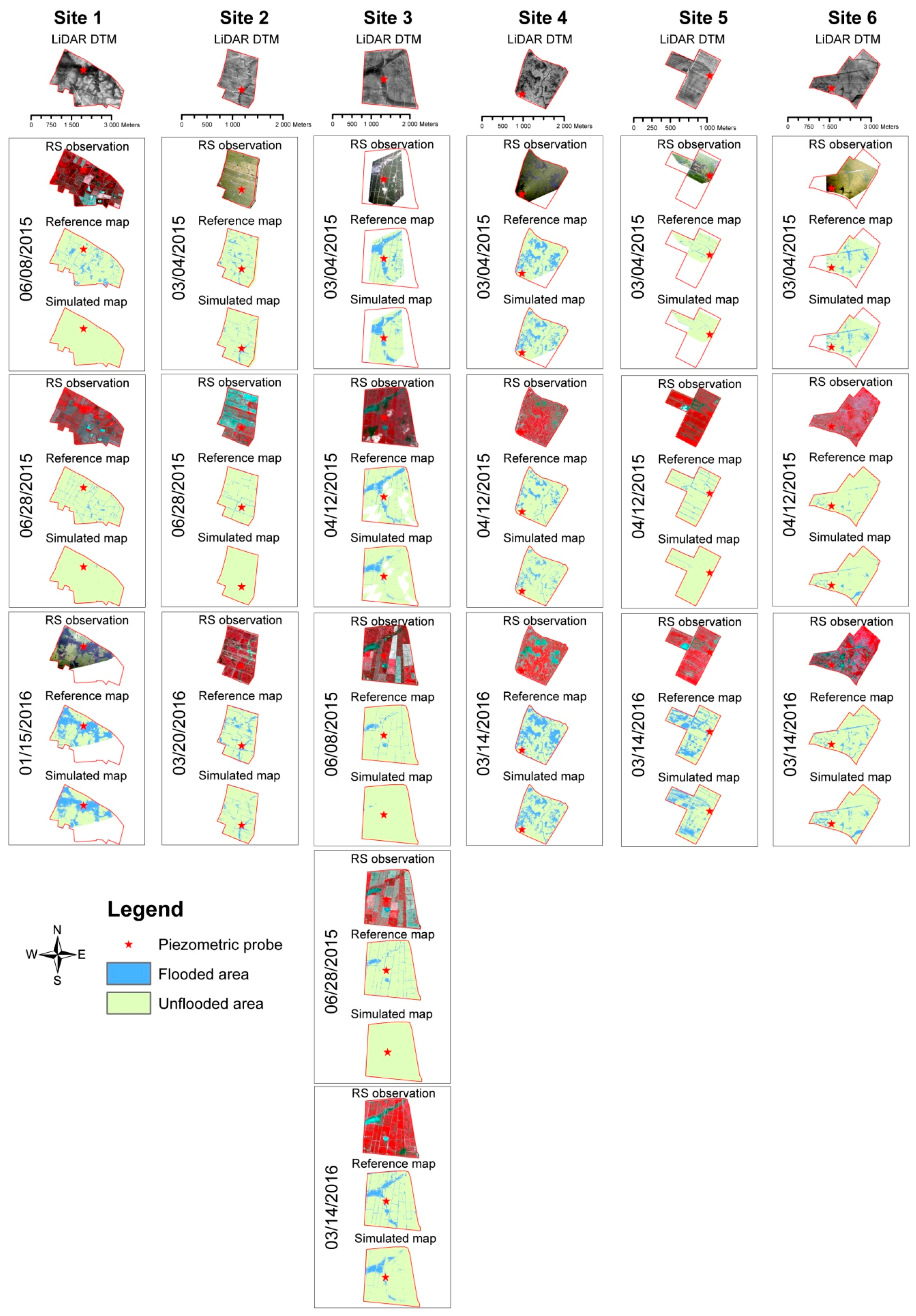
3.1. Accuracy Assessment

The median LiDAR-based DTM altimetry errors (i.e., offset) ranged from 6 cm to 26 cm, depending on the site (Figure 2). The minimum and maximum altimetry errors were found on sites 5 and 1, respectively. For sites 2, 3, 4, and 6, the values for the median errors were similar, and ranged from 16 cm to 19 cm. The standard deviation errors ranged from 6.5 (site 5) to 14.6 (site 6) cm, and revealed a moderate error variability within the sites. For site 1, the higher altimetry errors could be explained by the vegetation cover (tall and dense grasslands, ~80 cm in height). The offset (i.e., median error) values applied for the calibration of the LiDAR-based DTMs are listed in Table 2.

Statistical comparisons between the maps of the flooded areas observed from the seven remote sensing images and the pattern simulated from the LiDAR data are shown in

Table 3. Calibration and validation results of the flooding simulation model (OA = overall accuracy index in %, K_loc = Kappa location index, na = remote sensing image not available).

		Site 1		Site 2		Site 3		Site 4		Site 5		Site 6
Calibration	Offset (cm)	26		18		18		16		06		19
Validation	Date	OA	Kloc	OA	Kloc	OA	Kloc	OA	Kloc	OA	Kloc	OA	Kloc
	4 March 2015	na	na	89.5	0.39	82.3	0.73	79.9	0.78	93.8	0.42	91.9	0.75
	12 April 2015	na	na	na	na	87.4	0.64	87.5	0.55	92.9	0.58	94.4	0.43
	8 June 2015	88.9	0.42	na	na	94.1	0.88	na	na	na	na	na	na
	28 June 2015	92.9	0.24	94.6	0.81	93.0	0.98	na	na	na	na	na	na
	15 January 2016	84.7	0.82	na	na	na	na	na	na	na	na	na	na
	14 March 2016	na	na	na	na	89.4	0.64	79.7	0.77	76.0	0.48	88.2	0.41
	20 March 2016	na	na	85.5	0.53	na	na	na	na	na	na	na	na
	Mean	88.8	0.49	89.9	0.58	89.2	0.77	82.3	0.70	87.6	0.49	91.5	0.53

. In general, the mean OA values ranged from 82.3% to 91.5%, and thus show that there is a good agreement between the simulations and the remotely-sensed observations, regardless of the site (Table 3). The analysis of the mean K_loc index also highlights the differences among the sites in terms of the error location. Mean K_loc values higher than 0.6 were found on sites 3 and 4—revealing a spatial concentration for the error location—whereas K_loc values lower than 0.6 were measured on sites 1, 2, 5, and 6—expressing a high spatial dispersion of the error. More specifically, a site-per-site interpretation highlights variations in the flood simulation performance among the seasons. On site 1, the OA values were excellent in both June (88.9–92.2%) and January (84.7%), and the K_loc index ranged from poor/moderate in June (0.24–0.42) to excellent values in January (0.82). On site 2, the OA values were excellent in both March (85.5–89.5%) and June (94.6%), and the K_loc index ranged from moderate values in March (0.39–0.53) to excellent values in June (0.81). On site 3, the OA values were excellent in March (82.3–89.4%), April (87.4%), or June (93.0–94.1%), and the K_loc index ranged from moderate values in March and April (0.64 for both) to excellent values in June (0.88–0.98). On site 4, the OA ranged from good values in March (79.7–79.9%) to excellent values in April (87.5%) while the K_loc index ranged from moderate values in April (0.55) to good values in March (0.77–0.78). On site 5, the OA ranged from good values in March 2016 (76%) to excellent values in March/April 2015 (93.8% and 92.9%, respectively) while the K_loc index values were moderate regardless of the date (0.42–0.58). Finally, on site 6, the OA values were excellent in either March or April (88.2–94.4%), while the K_loc index ranged from moderate values in April 2015 and March 2016 (0.43 and 0.41, respectively) to good values in March 2015 (0.75).

As a general trend, the observed and simulated flood extents showed a high level of similarity, in accordance with the OA and K_loc values (Figure 3). More specifically, two situations were recorded. Firstly, during the period when grasslands were dry and water was only present in ditches and permanent ponds on the reference maps (e.g., 28 June 2015 for sites 1–3 or 12 April 2015 for site 5), the flooded simulated extent was nearly null in the grasslands, as well as in the ditches and permanent ponds. These errors can be explained by the presence of water in the ditches and permanent ponds at the time of the LiDAR acquisition, which is an obstacle to LiDAR signal penetration, and therefore to microtopographic characterization. Secondly, when the sites were widely flooded (e.g., 15 January 2016 for site 1, or 14 March 2016 for sites 4–5), then, the fine-scale spatial patterns of the flooded areas were found to be reliably simulated, regardless of whether the flooding occurred in large depressions or in narrow ditches. In this situation, the simulation performs well, even several hundred meters away from the piezometric probe. However, some underdetection errors could be noticed (e.g., 4 March 2015 on site 2, and in the eastern part of site 3), which was probably related to the altimetric error of the LiDAR DTM in relation to the vegetation cover (tall and dense grasslands, ~80 cm in height).

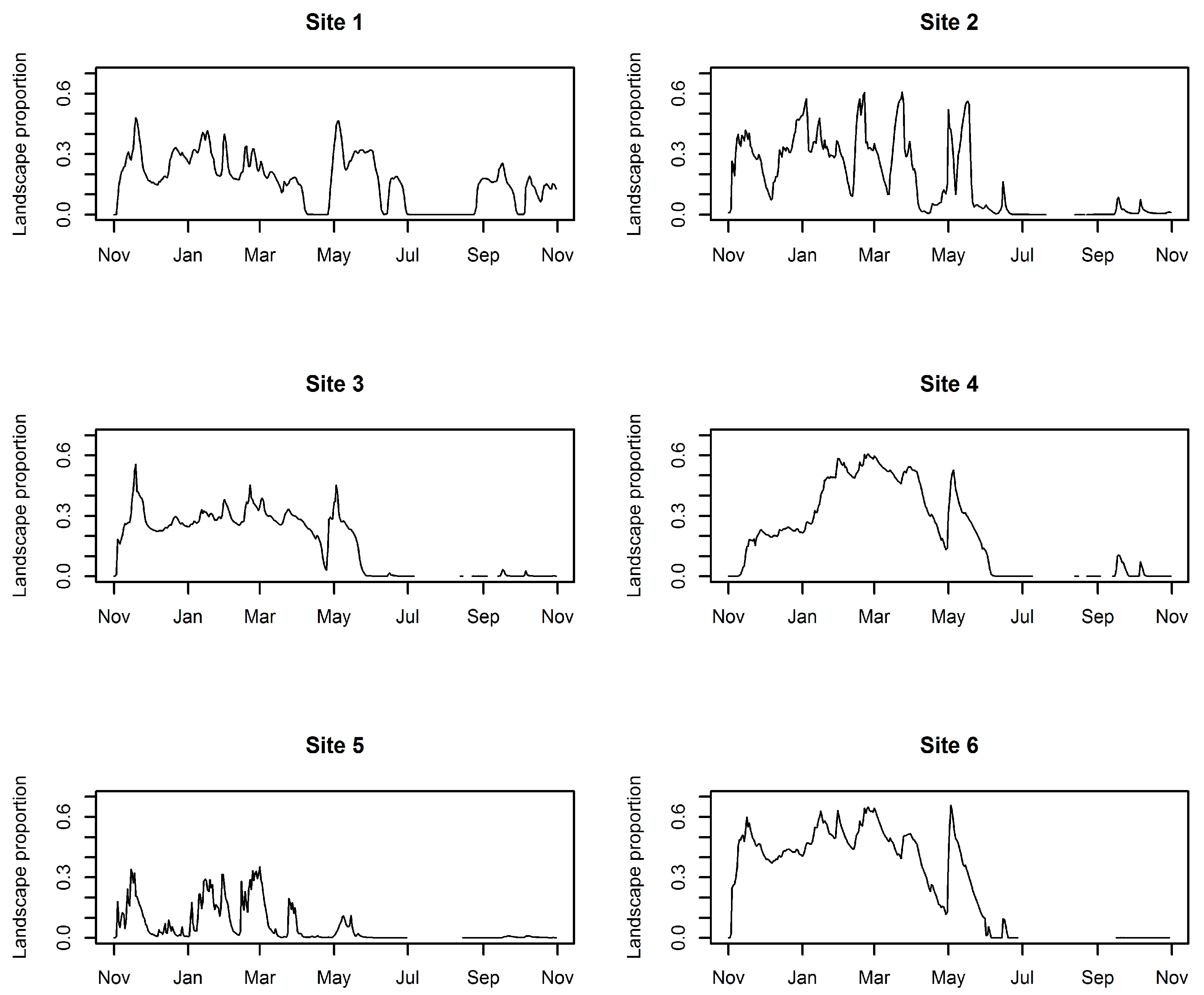
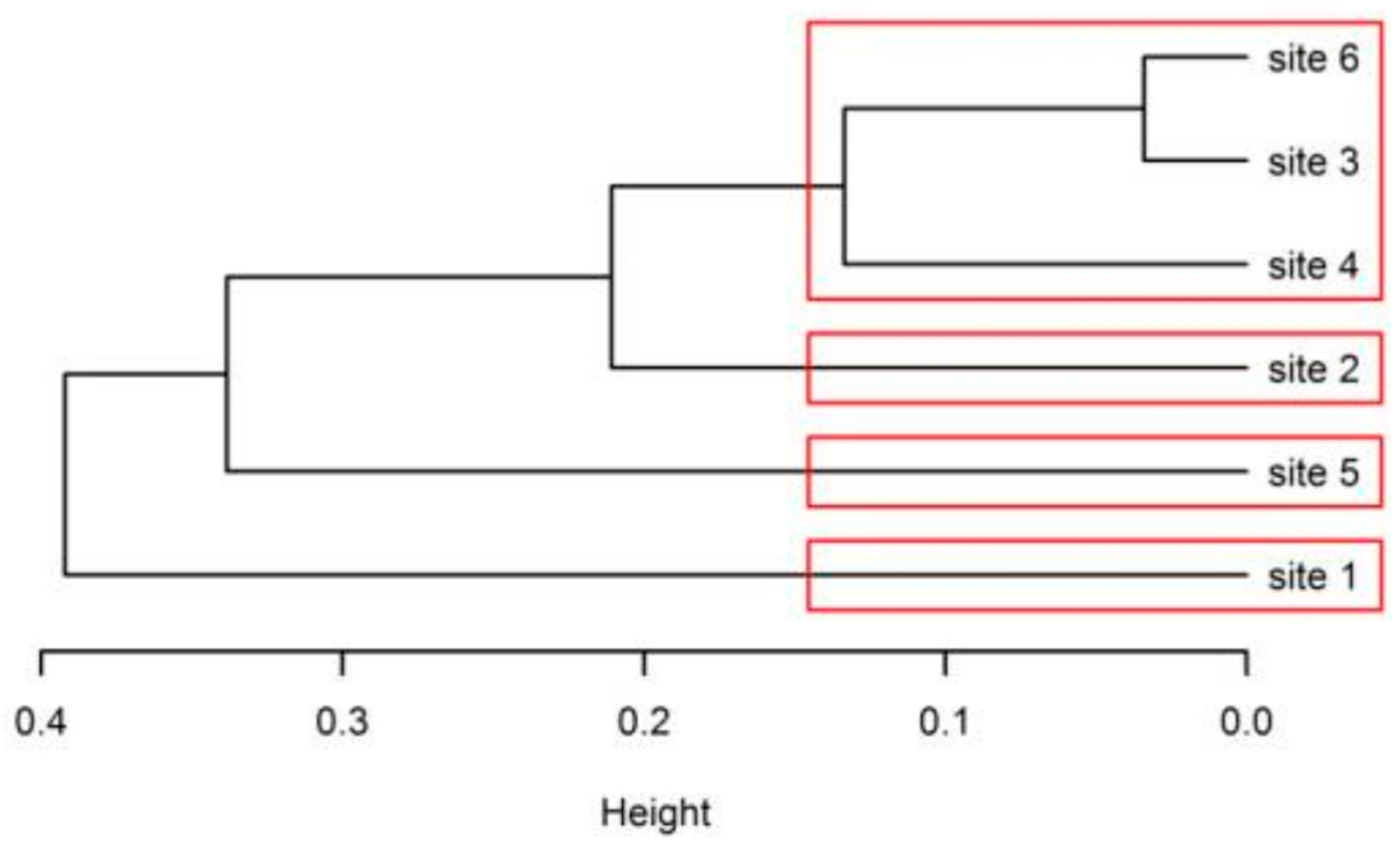
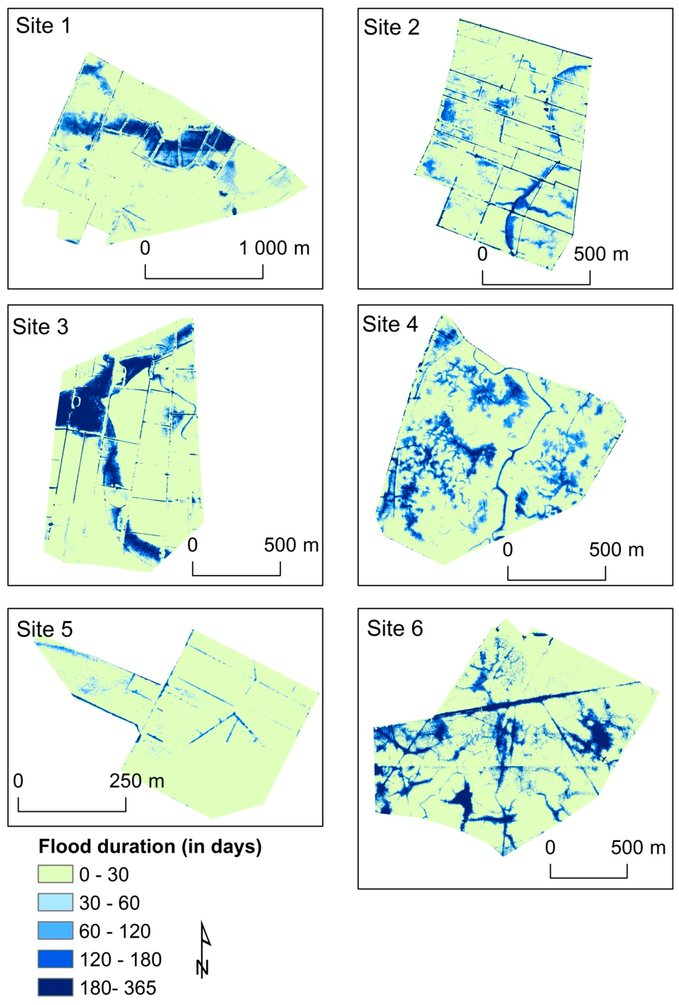
3.2. Spatiotemporal Characterization of the Flood Patterns

The LPI analyses showed that the flooding events generally occurred between November 2014 and June 2015 (Figure 4). Within this general pattern, a fine temporal variability of the LPI can be noticed, particularly on sites 2–5. The highest LPI values can be seen on sites 4–6. The flood extents became restricted in summer and autumn, except on site 1, where the LPI increased again from September onward.

The comparison of the hydrological behavior between the sites is presented in Figure 5. Based on the visual inspection of the dendrogram, we chose to set the threshold distance value to 0.15. Sites 1, 2, and 5 are classified into three different clusters, while sites 3, 4, and 6 are grouped within a common cluster.

The map of the annual flooded duration was produced for all of the sites (Figure 6). Even within the limited altitudinal gradient (<1 m), large variations in the annual flood duration were found, ranging from 0 for the upper locations, and up to 365 days for the lower areas. On sites 1–3, the longest flooded areas (>180 days a year) were located in paleochannels with pronounced depressions (>50 cm). However, the situation was quite different on sites 4–6, where the longest flooded areas occurred and where the water was lengthily retained by managements that may not only have been in the deeper depressions. Overall, the annual flood durations were lower on site 2 (60–120 days), and especially on site 5 (0–30 days), where a dense ditch network may have efficiently drained the water.

In order to illustrate the fine-grained and sinuous shape of the flooded areas in the studied coastal marshland, Figure 7 focused on site 4, which shows the typical patterns in the region. Each pixel is characterized by its temporal flooding profile. As an example, three temporal profiles were extracted from three plots (i.e., pixels) chosen along a fine—i.e., 40-cm large—elevation gradient. These results showed that the differences in the flood duration among the sites mainly occurred during late spring and early summer. In addition, a high variability in the flood duration can be observed between plots even only a few meters away. Plot 1, which was situated on a higher elevation, was flooded for 92 days from January to April; whereas plot 2, which was located at an intermediate elevation, was flooded for 143 days, from January to June; and Plot 3, located at a lower elevation, was flooded for 216 days, from November to July.

4. Discussion

4.1. Model Performance and Limitations

The calibration of the predictive model of the flooding extent was based on a constant offset value that was related to the median altimetry error of the LiDAR-based DTM. The comparison between the DGPS measurements and DTM pixels showed strong similarities in terms of the elevation values (a variation of 10 centimeters in the altimetry errors). Although some differences higher than 10 cm were observed in the dense herbaceous vegetation and shallow water bodies, this finding corroborates with previous studies [15,28]. To minimize the altimetric error of the LiDAR-based DTM, we tested the effect of applying a plant species-specific offset; this correction by plant height was shown to be efficient, although it may not have fully balanced the errors: the post-correction accuracy assessments reached a mean altimetric error of ~20cm in the salt marshes [39]. This remaining altimetric error may partially explain part of the errors in the flooding simulations we produced, while no statistically significant relationship was found between the LiDAR altimetry error and the accuracy of the simulated flooding areas. As an example, sites 1 and 5 respectively had high (26 cm) and low (6 cm) median LiDAR altimetry errors, but similar OA values (88.8% and 87.6% respectively). Variations in the K_loc values appeared to be strongly correlated to the ditch density. On sites 2, 3, and 5, where the K_loc values were the lowest in the winter period, the ditch density was the highest. On the contrary, sites 1, 4, and 6, where the K_loc values were the highest in the winter period, showed the lowest density of ditches. These findings confirm previous studies that highlighted the ditch network density as an important control variable in hydrological processes in wet grasslands [1,26].

The validation of the model was based on seven remote sensing images acquired between late winter and early summer. This is a critical period in temperate wetlands in terms of the large variations occurring in the flood extent [10] and plant growth dynamics [4]. The results showed the good quality of the predictions made by the model we used, as the OA values ranged between 76–94%. Compared to the in situ validation, this approach presents some pros and cons. The first limitation concerns the use of three-date reference data per site: as a consequence, we assumed that this relationship between the piezometric altimetry value and flooded areas is globally constant throughout the year. With respect to the complex hydrological processes occurring in both the surface water and groundwater [1,40], this assumption could be considered simplistic. Additional data, spread out throughout the year, are needed in order to better calibrate the model and take the variation in the piezometric altimetry values and the preduction of flooded areas into account. Recently, Keys et al. [41] developed a cost-effective approach that was based on the use of a camera placed on top of a 10-m high field tower, which records hourly time-step images. Another large-scale efficient alternative could be the use of a new SAR time series. Recently, Cazals et al. [10] showed that flooded areas may be readily detectable in the Marais Poitevin (100,000 ha) using a 10-day revisit frequency for the Sentinel-1 satellite time series, at the regional scale. However, this work highlighted the limits of the radar data: flooded areas lower than 0.8 ha and/or shallow water with emergent vegetation were poorly detected, whereas they are actually very frequent in wetlands. On the contrary, the LiDAR-based simulations were able to successfully produce a daily fine-grained pattern characterization, but were constrained on sites measuring only a few hectares. In a nutshell, the observed and simulated approaches appeared to be complementary, since they were suitable for regional/monthly and local/daily scales, respectively.

The second limitation lies in the possible visual misinterpretations of the flood extents of the remotely sensed data that were used to establish the reference flooding maps. Hence, we assumed that the flooded areas were detected with a minimum water depth of 15 cm, which is relevant based on our field knowledge; however, this water depth threshold may locally underdetect or overdetect the flooding areas that were covered by vegetation taller than 30 cm or smaller than 10 cm.

Conversely, the main advantage of the approach proposed here is its significant spatial sampling based on a raster reference map, including hundreds of pixels (i.e., validation samples). The reference map offers the opportunity to calculate a K_loc index, which assesses the spatial dispersion of the error, and is well adapted (better than the Kappa index) for the assessment of the simulated map [36]. Another interest of the method used here is that the errors on the simulated maps can be spatialized: the comparison between the reference maps showed that the simulated maps were correctly modeled, and not only close to the piezometric probe, but also hundreds of meters away.

In contrast to hydrological models that require a high level of expertise and intensive data acquisition [40], the model we developed, which was based on LiDAR and piezometric data, is simple and suitable for mapping both surface and subsurface water with spatially fine-grained precision across many hectares. Our results underlined how microtopography data may be useful and help predict flooding in wetlands [22,42].

It should also be noticed that while many studies have pointed out the importance of a hydrological network [19], vegetation resistance [18,20,21,42], and infiltration [23] in flow modeling, these factors were not considered here, and could explain some errors in our simulation. However, the integration of these factors in hydrological modeling remains challenging for three reasons. Firstly, we acknowledge that the hydrological connectivity between wet grasslands and the hydrological network is crucial for assessing wetland functions [19], but this connectivity is difficult, perhaps even impossible, to be reliably assessed since floodplains are connected through small intermittent creeks or waterflows that are not captured by LiDAR data [25]. Recently, McDonough et al. [43] suggested monitoring the surface hydrologic connectivity between wetlands and streams with a float switch data logger system. The coupling of this system with the use of both LiDAR and piezometric data, as done in this study, would provide a great way to monitor the effective connection/disconnection pattern in time and space. Alternatively, this limitation could be circumvented by using new bathymetric LiDAR data, which are suitable for capturing channel beds [44]. Secondly, the vegetation resistance is highly variable in time in relation to the growing season, and the somewhat unreliable inputs from these parameters could be another source of errors, rather than a significant improvement [42]. Thirdly, the infiltration parameter is difficult to spatialize at the fine scale with sufficient certainty. The integration of remotely-sensed SAR (such as TerraSAR-X) time series in flood inundation models could provide promising avenues for mapping flood hazards and overland flows [10,13].

4.2. Toward a Better Knowledge of Ecohydrological Processes

The daily simulation of fine-grained flood patterns in wet grasslands offers a relevant technical and methodological solution for a real-time ecohydrology [45]. For example, this approach is able to detect rapid changes in the characteristics of the signal “pulse” based on the LPI value, as in site 6 in May (Figure 4). Considering the flood duration map (Figure 7), areas with significant changes compared to their surroundings can be identified, and considered “hot spots” [45]. Some “thresholds” can be highlighted in May, when small changes in the water management led to an abrupt decrease in the extent of the flooded areas (Figure 4). Such abrupt variations in spring, when reproduction is occurring for most of the flora and fauna, may present strong consequences for the biodiversity patterns. Interestingly, the hierarchical clustering of the LPI time series highlighted a common cluster including all three sites concerned by conservation planning for waterbirds, which are generally accompanied by a longer flooding period in the spring (Figure 5).

In this study, the water levels measured by the piezometric probes result from both natural (precipitation and evapotranspiration) and anthropogenic drivers (water management). Although the daily-step flooded maps provide interesting information for local managers, the real impacts of water management on flooded areas remain unclear with regard to climatic conditions. The recent development of an interactive simulation tool to promote adaptation to climate variability [6] constitutes an interesting track to follow in order to discriminate the respective contributions of natural and anthropogenic variables on the water level dynamics.

There will be many applications for the inundation map that has been produced, in particular in the fields of plant and animal ecology. Regarding plant biodiversity and communities, it will provide needed information for predicting the distribution of plant species and communities [46], as well as plant functional traits and species richness, as shown by Violle et al. [4]. Our simulated map of flooding at a daily step could explore this relationship with a larger environmental characterization of the flood patterns and a more in-depth characterization of the key time period and interannual variations. Within each site, the differences in the annual flood duration were mainly related to contrasts occurring in narrow intervals both in time (two months) and topography (40 cm).

The modeling of the daily flooded areas over a one-year period, over 661 ha, with a 1 m × 1 m spatial resolution produces a huge amount of data (>7 GB). It could be interesting to carry out advanced analyses, such as the classification of pixels based on their temporal profiles. However, the spatial and temporal analyses of these large datasets are still challenging, and require further algorithmic and computational developments [47].

5. Conclusions

In this study, we modeled the flooding pattern in wet and highly drained grasslands with both fine temporal precision (one day) and on a fine spatial scale (one m). The model was built considering both LiDAR and in situ piezometric data. The comparison with the remote sensing-based reference maps showed that the model produces a good quality prediction. Better results were observed on the sites with a low ditch density (54–87 m/ha); whereas the highly drained sites (163–233 m/ha) showed a discrepancy with the model predictions. Further modeling developments that couple LiDAR data and drainage networks will be needed in order to improve the accuracy of the flood simulation in the high drained wet grasslands. The maps of the model outputs provide fine-grained maps showing the flooding and drying-out pattern of the shallow water patches. On this basis, the relationships between biodiversity and flooding dynamics may be studied, together with their respective spatial patterns.

References

1. Maltby, E.; Barker, T. The Wetlands Handbook; Wiley-Blackwell: Oxford, UK, 2009. [Google Scholar]
2. Acreman, M.; Holden, J. How wetlands affect floods. Wetlands 2013, 33, 773–786. [Google Scholar] [CrossRef]
3. Surridge, B.W.J.; Heathwaite, A.L.; Baird, A.J. Phosphorus mobilisation and transport within a long-restored floodplain wetland. Ecol. Eng. 2012, 44, 348–359. [Google Scholar] [CrossRef]
4. Violle, C.; Bonis, A.; Plantegenest, M.; Cudennec, C.; Damgaard, C.; Marion, B.; Le Cœur, D.; Bouzillé, J.-B. Plant functional traits capture species richness variations along a flooding gradient. Oikos 2011, 120, 389–398. [Google Scholar] [CrossRef]
5. Żmihorski, M.; Pärt, T.; Gustafson, T.; Berg, Å. Effects of water level and grassland management on alpha and beta diversity of birds in restored wetlands. J. Appl. Ecol. 2016, 53, 587–595. [Google Scholar] [CrossRef]
6. Lefebvre, G.; Germain, C.; Poulin, B. Contribution of rainfall vs. water management to Mediterranean wetland hydrology: Development of an interactive simulation tool to foster adaptation to climate variability. Environ. Model. Softw. 2015, 74, 39–47. [Google Scholar] [CrossRef]
7. Dash, J.; Ogutu, B.O. Recent advances in space-borne optical remote sensing systems for monitoring global terrestrial ecosystems. Prog. Phys. Geogr. 2016, 40, 322–351. [Google Scholar] [CrossRef]
8. Yan, K.; Di Baldassarre, G.; Solomatine, D.P.; Schumann, G.J.-P. A review of low-cost space-borne data for flood modelling: Topography, flood extent and water level. Hydrol. Process. 2015, 29, 3368–3387. [Google Scholar] [CrossRef]
9. Marti-Cardona, B.; Dolz-Ripolles, J.; Lopez-Martinez, C. Wetland inundation monitoring by the synergistic use of ENVISAT/ASAR imagery and ancilliary spatial data. Remote Sens. Environ. 2013, 139, 171–184. [Google Scholar] [CrossRef]
10. Cazals, C.; Rapinel, S.; Frison, P.-L.; Bonis, A.; Mercier, G.; Mallet, C.; Corgne, S.; Rudant, J.-P. Mapping and characterization of hydrological dynamics in a coastal marsh using high temporal resolution sentinel-1A images. Remote Sens. 2016, 8, 570. [Google Scholar] [CrossRef]
11. Malinowski, R.; Höfle, B.; Koenig, K.; Groom, G.; Schwanghart, W.; Heckrath, G. Local-scale flood mapping on vegetated floodplains from radiometrically calibrated airborne LiDAR data. ISPRS J. Photogramm. Remote Sens. 2016, 119, 267–279. [Google Scholar] [CrossRef]
12. Malinowski, R.; Groom, G.; Schwanghart, W.; Heckrath, G. Detection and delineation of localized flooding from worldview-2 multispectral data. Remote Sens. 2015, 7, 14853–14875. [Google Scholar] [CrossRef]
13. Bates, P.D. Integrating remote sensing data with flood inundation models: How far have we got? Hydrol. Process. 2012, 26, 2515–2521. [Google Scholar] [CrossRef]
14. Jung, Y.; Merwade, V. Uncertainty quantification in flood inundation mapping using generalized likelihood uncertainty estimate and sensitivity analysis. J. Hydrol. Eng. 2012, 17, 507–520. [Google Scholar] [CrossRef]
15. Hopkinson, C.; Chasmer, L.E.; Sass, G.; Creed, I.F.; Sitar, M.; Kalbfleisch, W.; Treitz, P. Vegetation class dependent errors in lidar ground elevation and canopy height estimates in a boreal wetland environment. Can. J. Remote Sens. 2005, 31, 191–206. [Google Scholar] [CrossRef]
16. Costabile, P.; Macchione, F.; Natale, L.; Petaccia, G. Flood mapping using LIDAR DEM. Limitations of the 1-D modeling highlighted by the 2-D approach. Nat. Hazards 2015, 77, 181–204. [Google Scholar] [CrossRef]
17. Maksimović, Č.; Prodanović, D.; Boonya-Aroonnet, S.; Leitão, J.P.; Djordjević, S.; Allitt, R. Overland flow and pathway analysis for modelling of urban pluvial flooding. J. Hydraul. Res. 2009, 47, 512–523. [Google Scholar] [CrossRef]
18. Ozdemir, H.; Sampson, C.; de Almeida, G.A.; Bates, P.D. Evaluating scale and roughness effects in urban flood modelling using terrestrial LIDAR data. Hydrol. Earth Syst. Sci. 2013, 10, 5903–5942. [Google Scholar] [CrossRef]
19. Bates, P.D.; Marks, K.J.; Horritt, M.S. Optimal use of high-resolution topographic data in flood inundation models. Hydrol. Process. 2003, 17, 537–557. [Google Scholar] [CrossRef]
20. Liu, Q.Q.; Singh, V.P. Effect of microtopography, slope length and gradient, and vegetative cover on overland flow through simulation. J. Hydrol. Eng. 2004, 9, 375–382. [Google Scholar] [CrossRef]
21. Özgen, I.; Teuber, K.; Simons, F.; Liang, D.; Hinkelmann, R. Upscaling the shallow water model with a novel roughness formulation. Environ. Earth Sci. 2015, 74, 7371–7386. [Google Scholar] [CrossRef]
22. Huang, S.; Young, C.; Feng, M.; Heidemann, K.; Cushing, M.; Mushet, D.M.; Liu, S. Demonstration of a conceptual model for using LiDAR to improve the estimation of floodwater mitigation potential of Prairie Pothole Region wetlands. J. Hydrol. 2011, 405, 417–426. [Google Scholar] [CrossRef]
23. Costabile, P.; Costanzo, C.; Macchione, F. A storm event watershed model for surface runoff based on 2D fully dynamic wave equations. Hydrol. Process. 2013, 27, 554–569. [Google Scholar] [CrossRef]
24. Yang, J.; Chu, X. A new modeling approach for simulating microtopography-dominated, discontinuous overland flow on infiltrating surfaces. Adv. Water Resour. 2015, 78, 80–93. [Google Scholar] [CrossRef]
25. Negishi, J.N.; Sagawa, S.; Sanada, S.; Kume, M.; Ohmori, T.; Miyashita, T.; Kayaba, Y. Using airborne scanning laser altimetry (LiDAR) to estimate surface connectivity of floodplain water bodies. River Res. Appl. 2012, 28, 258–267. [Google Scholar] [CrossRef]
26. Lang, M.; McDonough, O.; McCarty, G.; Oesterling, R.; Wilen, B. Enhanced detection of wetland-stream connectivity using lidar. Wetlands 2012, 32, 461–473. [Google Scholar] [CrossRef]
27. Hauer, C.; Mandlburger, G.; Schober, B.; Habersack, H. Morphologically related integrative management concept for reconnecting abandoned channels based on airborne lidar data and habitat modelling. River Res. Appl. 2014, 30, 537–556. [Google Scholar] [CrossRef]
28. Džubáková, K.; Piégay, H.; Riquier, J.; Trizna, M. Multi-scale assessment of overflow-driven lateral connectivity in floodplain and backwater channels using LiDAR imagery. Hydrol. Process. 2015, 29, 2315–2330. [Google Scholar] [CrossRef]
29. Shook, K.; Pomeroy, J.W.; Spence, C.; Boychuk, L. Storage dynamics simulations in prairie wetland hydrology models: Evaluation and parameterization. Hydrol. Process. 2013, 27, 1875–1889. [Google Scholar] [CrossRef]
30. Cazorzi, F.; Fontana, G.D.; Luca, A.D.; Sofia, G.; Tarolli, P. Drainage network detection and assessment of network storage capacity in agrarian landscape. Hydrol. Process. 2013, 27, 541–553. [Google Scholar] [CrossRef]
31. Maclean, I.M.D.; Bennie, J.J.; Scott, A.J.; Wilson, R.J. A high-resolution model of soil and surface water conditions. Ecol. Model. 2012, 237, 109–119. [Google Scholar] [CrossRef]
32. Duncan, P.; Hewison, A.J.M.; Houte, S.; Rosoux, R.; Tournebize, T.; Dubs, F.; Burel, F.; Bretagnolle, V. Long-term changes in agricultural practices and wildfowling in an internationally important wetland, and their effects on the guild of wintering ducks. J. Appl. Ecol. 1999, 36, 11–23. [Google Scholar] [CrossRef]
33. Council Directive 92/43/EEC Conservation of natural habitats and of wild flora and fauna. Int. J. Eur. Commun. 1992, L206, 7–49.
34. Laben, C.A.; Brower, B.V. Process for Enhancing the Spatial Resolution of Multispectral Imagery Using Pan-Sharpening. U.S. Patent US6011875, 4 January 2000. [Google Scholar]
35. Blaschke, T. Object based image analysis for remote sensing. ISPRS J. Photogramm. Remote Sens. 2010, 65, 2–16. [Google Scholar] [CrossRef]
36. Pontius, R.; Millones, M. Death to Kappa: Birth of quantity disagreement and allocation disagreement for accuracy assessment. Int. J. Remote Sens. 2011, 32, 4407–4429. [Google Scholar] [CrossRef]
37. Paparrizos, J.; Gravano, L. K-Shape: Efficient and Accurate Clustering of Time Series. In Proceedings of the 2015 ACM SIGMOD International Conference on Management of Data (SIGMOD ’15), Melbourne, Australia, 31 May–4 June 2015; ACM: New York, NY, USA, 2015; pp. 1855–1870. [Google Scholar]
38. Sarda-Espinosa, A. Dtwclust: Time Series Clustering Along with Optimizations for the Dynamic Time Warping Distance. Available online: https://cran.r-project.org/web/packages/dtwclust/index.html (accessed on 28 February 2018).
39. Hladik, C.; Alber, M. Accuracy assessment and correction of a LIDAR-derived salt marsh digital elevation model. Remote Sens. Environ. 2012, 121, 224–235. [Google Scholar] [CrossRef]
40. Golden, H.E.; Lane, C.R.; Amatya, D.M.; Bandilla, K.W.; Raanan Kiperwas, H.; Knightes, C.D.; Ssegane, H. Hydrologic connectivity between geographically isolated wetlands and surface water systems: A review of select modeling methods. Environ. Model. Softw. 2014, 53, 190–206. [Google Scholar] [CrossRef]
41. Keys, T.A.; Jones, C.N.; Scott, D.T.; Chuquin, D. A cost-effective image processing approach for analyzing the ecohydrology of river corridors. Limnol. Oceanogr. Methods 2016, 14, 359–369. [Google Scholar] [CrossRef]
42. Kadlec, R.H. Overland flow in wetlands: Vegetation resistance. J. Hydraul. Eng. 1990, 116, 691–706. [Google Scholar] [CrossRef]
43. McDonough, O.T.; Lang, M.W.; Hosen, J.D.; Palmer, M.A. Surface hydrologic connectivity between delmarva bay wetlands and nearby streams along a gradient of agricultural alteration. Wetlands 2014, 35, 41–53. [Google Scholar] [CrossRef]
44. Legleiter, C.J.; Overstreet, B.T.; Glennie, C.L.; Pan, Z.; Fernandez-Diaz, J.C.; Singhania, A. Evaluating the capabilities of the CASI hyperspectral imaging system and Aquarius bathymetric LiDAR for measuring channel morphology in two distinct river environments. Earth Surf. Process. Landf. 2016, 41, 344–363. [Google Scholar] [CrossRef]
45. Krause, S.; Lewandowski, J.; Dahm, C.N.; Tockner, K. Frontiers in real-time ecohydrology—A paradigm shift in understanding complex environmental systems. Ecohydrology 2015, 8, 529–537. [Google Scholar] [CrossRef]
46. Wassen, M.J.; Peeters, W.H.M.; Venterink, H.O. Patterns in vegetation, hydrology, and nutrient availability in an undisturbed river floodplain in Poland. Plant Ecol. 2003, 165, 27–43. [Google Scholar] [CrossRef]
47. Ma, Y.; Wu, H.; Wang, L.; Huang, B.; Ranjan, R.; Zomaya, A.; Jie, W. Remote sensing big data computing: Challenges and opportunities. Future Gener. Comput. Syst. 2015, 51, 47–60. [Google Scholar] [CrossRef]
Figure 1. Location of the study sites and field photography showing the shallow water in the grasslands.
Sustainability 10 00708 g001
Figure 2. Light detection and ranging (LiDAR)-based digital terrain model (DTM) altimetry error according to the site (differential global positioning system (DGPS) plot numbers per site are shown above their respective boxplot).
Sustainability 10 00708 g002
Figure 3. LiDAR DTM; reference and simulated flood map derived from a remote sensing observation and LiDAR DTM, respectively.
Sustainability 10 00708 g003
Figure 4. One dynamic of the flood patterns, measured as the landscape proportion index covered with simulated water along a one-year hydrological cycle.
Sustainability 10 00708 g004
Figure 5. Dendrogram produced from the agglomerative clustering analysis of the flooded landscape proportion index (LPI) time series (shape-based distance) per site.
Sustainability 10 00708 g005
Figure 6. Maps of the annual flood duration for all of the sites.
Sustainability 10 00708 g006
Figure 7. Annual flood duration map for site 4 and selected temporal profiles.
Sustainability 10 00708 g007