Is the High Interest Rate Combined with Intense Deleveraging Campaign Desirable? A Collateral Mechanism under Stringent Credit Constraints

Abstract

Recently, China has witnessed a continuously increasing Debt-to-GDP ratio and a vigorously expanding shadow banking sector. Housing prices hovering at a high level seriously affect the lives of ordinary residents. Disappointingly, a variety of activities such as intense deleveraging campaigns and tight monetary controls produce little effect. Why do these seemingly rightful implementations hardly work? What should governments do to stop the incessant expansion of asset bubbles? What role ought financial supervisors to play in regulating credit markets and facilitating a sustainable and inclusive economic growth? This paper sets off from the pledgeability of asset bubbles and constructs a generalized overlapping generation (OLG) model incorporating financial frictions and collateral constraints, in order to explore the bubble evolution under the alterations of market interest rates and credit conditions. The results show a unique bubble equilibrium, in which the steady-state bubble size expands when interest rate increases. Numerical results further reveal that the bubble-inflation effect of a higher interest rate is reinforced by a more stringent collateral constraint. Our research contributes to an explanation of the inefficacy of present policies and provides the following policy implications: The combination of an interest rate elevation and a strong loan restriction is in fact undesirable for suppressing asset bubbles. Not merely does it strike productivity and capital formation, but it also fosters investors to hold more risky assets to solve liquidity shortage under constrained borrowing capacity.

1. Introduction

After the 2008 global financial crisis, both the housing market and the stock market all over the world showed drastic fluctuations in asset prices, in a general background of an imperfect credit environment. Should government strengthen policy control to manage inflated asset bubbles? Can a rise in interest rate hold down bubbles efficiently and can contractionary policy implementations mitigate any economic downturn? This ostensibly reasonable belief has reached a general consensus in theory and practically guides the interventions and supervisions in financial markets for years. Nevertheless, there have been dozens of counterexamples of a “price puzzle” where stringent interest rate policy pushes up asset prices and inflates bubbles, which has drawn public attention.

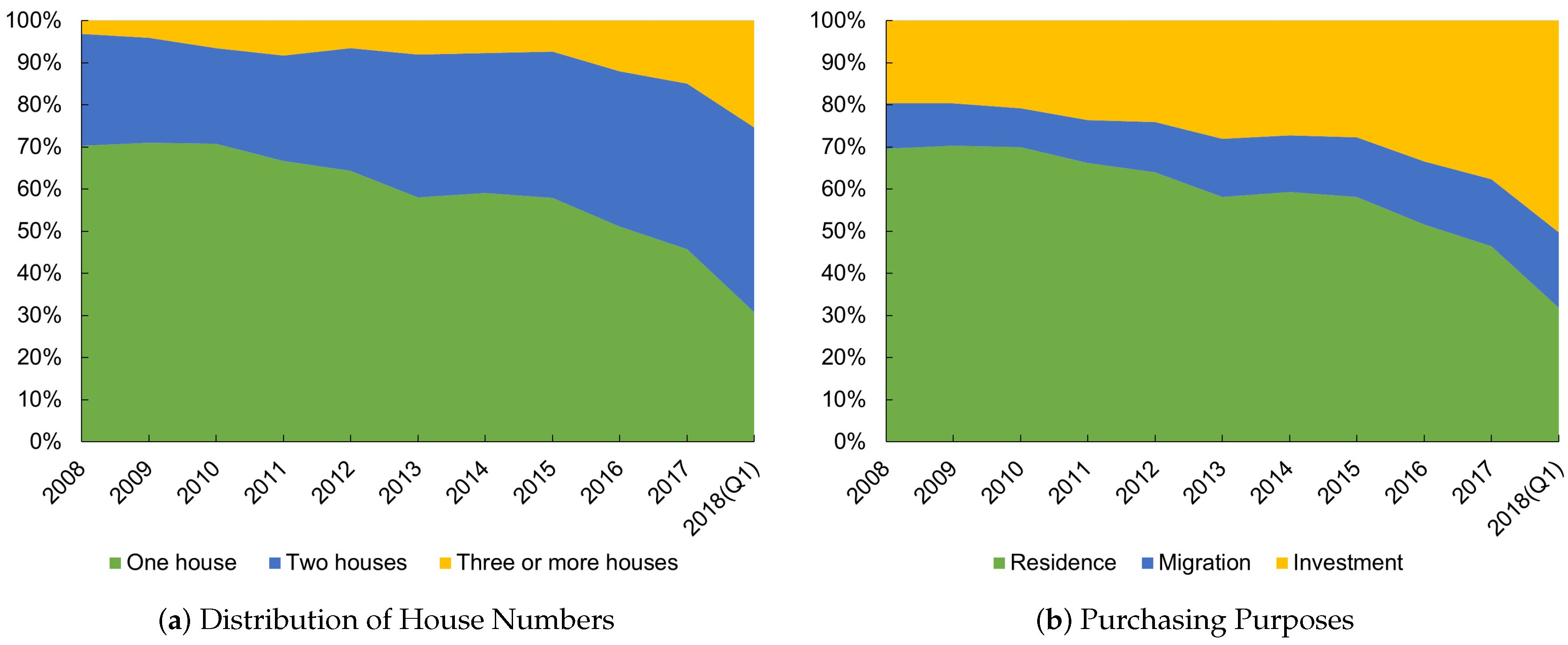
At the same time, in China, in face of the soaring housing prices and the over-leveraged financial systems of recent years, the Chinese government and the People’s Bank of China have been responding actively and taking varying measures to harness booming bubbles. On the quantity side, the government has put forward a series of control policies including home-purchasing limits and property-loan restrictions. On the price side, the central bank has continuously raised reverse repo rates and has even directly lifted loan interest rates. The ex post facto effects, however, are by no means satisfactory. In the past decade, real estate properties have been disproportionately purchased by investors who already own houses, vividly displayed in Figure 1a. Taking a close look at their purchasing reasons according to the nationally representative China Household Finance Survey (CHFS), Figure 1b manifests a clear purpose of speculation and an unstoppable build-up of leverage in real estate markets.

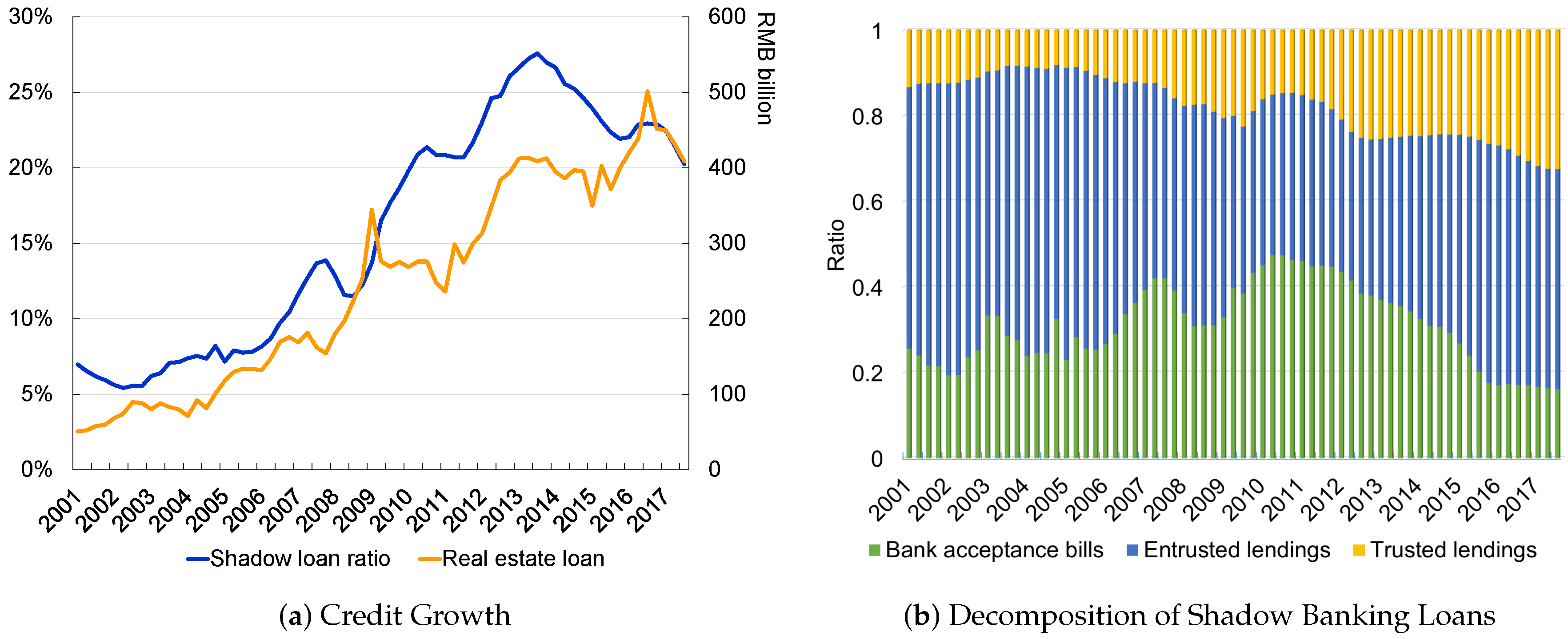
Despite the upsurge bubbles in housing markets, emerging issues in debt markets put financial supervisors in a difficult position, since the austerity measures they implemented and the deleveraging campaign they launched were substantially criticized for their ineffectiveness. A quick glimpse at Figure 2 is enough to view the ever-increasing debt burden and the unsatisfactory situations of China’s credit market. The quarterly data in Figure 2 is extracted from the dataset of China’s macroeconomic time series constructed for [1], which is a perfect and comprehensive collection of the raw data from China’s National Bureau of Statistics and Ministry of Finance and the People’s Bank of China.

Starting from 2001, two time series of shadow loan ratios and real estate loans present an overwhelming growth pattern of credit scale in Figure 2a. If we examine the shadow banking loan in its subdivisions of bank acceptance bills, entrusted lendings, and trusted lendings, Figure 2b clearly reveals the aggressive expansion of trust and entrust loans not included in the balance sheets, which for this reason implicitly hides default risks to a large extent and creates ascending leverage in financial systems. Until 2018, the proportion of bank acceptance bills has shrunk to 16%, from the summit point of 47% in 2011.

In a long-term sustainable financial system, moderate leverage ratios and stable asset prices are essential to minimize systematic risks and achieve the goal of steady development. In particular with regard to the real estate market, a small or moderate bubble implies that housing price faithfully reflect fundamental, so that common residents find it easy to make rational migration decisions and so that construction enterprises make good use of energy resources. The alternative scenario is more worrying: Unexpected market prices mislead urban change, unavoidably causing a loss to agricultural land that could have been optimally allocated and efficiently utilized for cultivation and afforestation.

Despite the best of intentions and efforts, as a matter of fact, neither the present strict control measures on real estate nor stringent market regulations on credit are of great advantage to the long-term sustainability and robust growth in housing markets, at least based on the evidence in China. Why does the contractionary monetary policy in a harsh credit environment fail to change these problematic situations? What role should financial supervisors play in regulating asset bubbles in the emergence of sustainable finance? These are all pretty significant issues worth addressing.

The contribution of this paper is summarized as follows. First, most of the scholars who follow housing bubbles with interest concentrate on the U.S. market, as in [2,3,4,5], yet unfortunately have not dug into the Chinese economy with enormous potential. In addition, among all the abundant research devoted to harness housing bubbles, previous scholars have seldom conducted a systemic study on the compound effect of a twofold austerity measure, featured by an upward interest rate and a rigid credit restriction. Our work contributes to the existing literature and adds to the above research gaps by investigating thoroughly the unintended consequences of this twofold policy measure and providing a plausible explanation for the unsolved real estate bubbles. Starting from the counter-intuitive phenomenon of the swelling asset bubble and deteriorated debt conditions under tight monetary policies and strong deleveraging operations in China’s financial market, this paper attempts to address this issue by developing a generalized overlapping generation (OLG) model in a standard New Keynesian framework, widely applied in the literature on asset markets and monetary policy.

Second, while the literature of monetary effects on asset prices is broad and sufficient, it lacks a thorough inquiry into one essential function of bubble assets: mortgage financing. This paper places particular emphasis on the pledgeability of rational asset bubbles in investor collateral composition and explores the effects of changes in market interest rates from the perspective of a collateral mechanism in monetary transmissions. As heated debates pay much attention to the growing risks posed by the bulky share of pledged real estates and accumulated liquidity pressures on borrowers, this work has practical relevance to the future sustainability and development of the Chinese financial market, which is closely bound up with the global economy at a higher level from the current situation.

Furthermore, we also make theoretical extensions on a few pioneering studies: We augment [6] by allowing entrepreneurs and general workers to hold bubbles. We also justify the crowd-out effect of bubbles on capital accumulation in [7,8]. Infinite-horizon models, e.g., [9,10,11], focus on the effects on investment and the allocation of stock price bubbles with positive dividends. Our work extends and modifies them by concentrating on the pure bubbles that serve as a store of value traded by overlapping agents, aiming at better fitting the reality of housing markets and evaluating the comprehensive influence in overlapping generations.

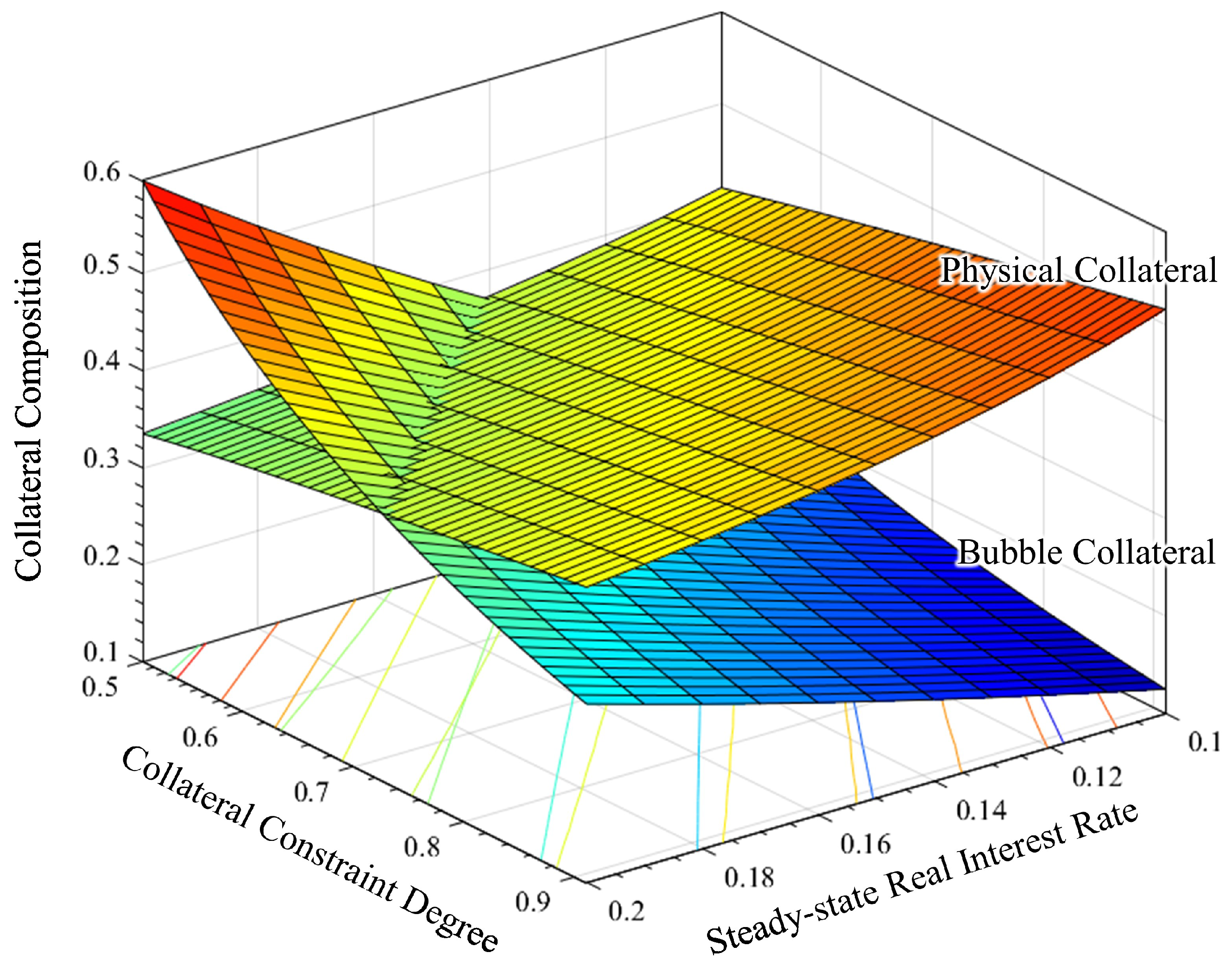
The line of reasoning in our logical framework processes is described below: Rational bubbles enter asset markets following [12] and serve as a portion of collaterals used for loan investment of entrepreneurs (henceforth referred to as “bubble collateral”). These intrinsically valueless assets produce no real payoff, expand when market return increases, and further appreciate with pledgeable feature. Meanwhile, on the production side, the correspondingly rising cost brought by increased interest rate hampers capital accumulation and production, depreciating the aggregate value of ordinary pledgeable assets (referred to as “physical collateral”). The composition of bubble and physical collaterals is utilized by representative investors in our model to satisfy their liquidity demand. In this situation, when investors bear stringent credit constraints and cannot borrow enough money with the available physical collateral, they will have motivations to add holdings for bubbles to alleviate the liquidity shortage. Additionally, taking the collateral mechanism in credit constraints into consideration, an intuitive inference extended here is that the above expansion effect of the rising interest rate on asset bubbles will be further reinforced if the borrowing restrictions become more rigid.

The rest of this paper is organized as follows: Section 2 summarizes related literature. Section 3 displays the stylized facts regarding bubbles and credit in China and empirical evidence with respect to a standard interest rate shock. Section 4 sets up the complete theoretical model considering credit frictions and bubble asset pledgeability. Section 5 discusses in detail the mathematical and numerical results, including the steady-state analysis of bubbly equilibrium, the comparative statics of collateral composition evolutions and impulse responses under the change in interest rates and the degree of credit frictions. Section 6 concludes, puts forward policy implications, and discourses limitations and future research. Appendix A and Appendix B contain technical proofs.

2. Literature Review

In view of the special nature of a speculative bubble generating no endogenous productivity, it is appropriate to regard it as an inherently valueless premium above price fundamental, within the scope of a pure rational bubble attached to positive price. In real transactions, dealers acknowledge that bubbles can burst in the unknown future. As is early illustrated in [13], the price of a speculative bubble is driven by the self-fulfilling mechanism of expectation. Bubbles expand as agents have confidence in sustained economic growth. With a rising risk premium and a rigid credit condition, continuous bubble inflation finally triggers a sudden collapse in investor sentiment and subsequently provokes a slump in financial markets. To make it worse, when we look into the real estate asset market specifically, a housing asset bears expensive transaction costs and confined short selling as a typical class of illiquid asset. As a factual matter, the frenzied overbuilding may be largely ascribed to an endogenous housing supply, well explained in [14]. A more inelastic housing supply breeds bubbles more easily, extends its duration, and exerts a profound impact on new construction and public welfare. In light of the grave consequences of bubble bursting, whether and how government and supervisors should react to asset bubbles have caused much controversy in academic and political circles.

Prior scholars who are in favor of tight policy have focused on the effects of the “reverse operation” on curbing the steep rise of asset prices, appeasing fluctuated financial markets and in this manner benefiting macro economic stability. The authors in [15] pointed out the ignorance of future price variations in the monetary policy regime of inflation targeting, and claimed that this weakness could be overcome by letting interest rates react to asset prices. Based on the theoretical framework of [16], the generation and evolution of bubbles have no influence on the future path of expected inflation, since rational agents perfectly anticipate that bubbles are destined to vanish in the future. Under this circumstance, the prevailing inflation targeting is invalid and could only apply “reverse operation” to asset prices so as to cool down the overheated economy. Soon after, the conference report of [17] speaks highly of the superiority of the “leaning against the wind” policy in regulating financial markets. Subsequent research in the Bank for International Settlements [18] and empirical evidence in Singapore [19] both back up this argument. Using a Bayesian likelihood approach, the supplement role of prompt policy adjustments to macro prudent policies has been well reflected in the estimated DSGE model in [20]. Similarly, the authors in [21] highlight the complementary effect of tight interest rates on banking supervision and regulation. Of recent years, in regard to some dissenting opinions of strict actions and market controls, the authors in [22] stress the far-reaching positive impacts on long-run sustained economic stability at the expense of sacrifice for the moment. Likewise, in a forthcoming theoretical study, the authors in [23] arrive at the conventional conclusion that a tightening policy control is optimal for decreasing bubble fluctuation.

In practice, however, numerous unsuccessful cases arouse suspicion for the actual effect of austerity campaigns. It is undeniable that a promotion of interest rate raises borrowing costs and harms material production. When the regulators do not have a clear knowledge of whether the climbing prices and red-hot economy stem from positive technological advances or bloated financial bubbles, a blind intervention for the purpose of stabilizing financial markets is very likely to generate the opposite outcome. The famous discussion in [24,25] conservatively advocates a “benign neglect” strategy when the economy confronts multiple shocks. This argument is soon supported and underlined by the authors in [26], who point out the possible scenario that one action aiming at quelling volatility in a certain market transfers pressure to other markets in the general equilibrium system and in the end disturbs market order through the feedback loop among market traders. Indeed, improper interference and credit squeeze can give rise to bubble collapses and the closely following violent aftermath of financial turmoil, discussed in detail by the authors in [27]. Fully aware of the great transformation with the advent of Economic and Monetary Union (EMU), the authors in [28] showed that demographic factors encourage housing bubbles to expand under relaxed financial constraints in Ireland and Spain. By virtue of the idiosyncrasy in housing markets across the Euro Area, the EMU monetary policy that targets the region as a whole barely works to control bubbles. For the sake of promoting sustainable economic growth associated with a compatible throughput rate not exceeding the carrying capacity of our finite planet, the authors in [29] call for the necessary restoration of money creation to support sufficient investment in pivotal public goods, with the cardinal aim of realizing the transition to a steady-state economy based on harmony and well-being. More recently, the authors in [12] account for the root reason why a rational asset bubble has a growth rate in accord with the market interest rate in partial equilibrium, and then set up a succinct and elegant general equilibrium model demonstrating that the design of an optimal monetary policy should judge and weigh the trade-off between bubble stabilization and inflation stabilization, and not only comply with the policy of “leaning against the wind.” Shortly after, this argument was further backed by empirical evidence in [30], which reveals an evolution pattern in the U.S. stock market that prices decrease when the economy is exposed to a tightened monetary policy. From the historical dimension looking back on the well known bubbles in the past 400 years, the authors in [31] summarize previous experiences and suggest that macro prudent measures, rather than strong interest rate tools, are more helpful to dampen bubble developments. In a comprehensive cost-and-benefit analysis, the authors in [32] arrive at the clear-cut conclusion that the marginal cost is much higher than the benefit for reverse operation in response to high asset prices. Apart from that, the authors in [33] indicate that government and supervisors substantially underestimate the extremely high costs produced by financial imbalances and policy misuse. Thus, the implementation of interest rate controls requires utmost caution.

In parallel with contractionary monetary policy, a very commonly used supplementary action is credit restriction. During the intense process of deveraging compaign, China has proposed rigorous rules regulating the financial industry, including enforcing specific liquidity requirements, shutting down peer-to-peer platforms and toughening supervision over micro lending firms. As a vital channel in the monetary transmission mechanism, credit supply is a topic of specific concern in the related literature. First explored in [34], the credit channel damages investment and production by diminishing productive collateral value and debt capacity. The full and accurate research in [35] elucidates how imperfection in credit markets accelerates monetary effects through the balance sheet and bank lending channels. Soon afterwards, plenty of research [36,37,38] presented corresponding dynamic models so as to clarify the amplification mechanism of financial frictions on adverse shocks to productivity. Two seminal papers [2,39] probed the credit effects in housing markets. The former demonstrated that collateral constraints attached to property values significantly magnify the aggregate demand responses to house price shocks and that debt indexation stabilizes supply shocks at the cost of amplifying demand shocks. The latter focused on the intervention of capital reallocation via collateral lending, giving emphasis to its influence on stochastic land bubbles in heterogeneous environments. As is uncovered by results in the extended real business cycle (RBC) model with financial shocks in [40], credit tightening plays an essential role in the recent three prominent recessions. Similarly in the infinite horizon models with endogenous credit constraints, the authors in [11,41] suggest that sound credit supply offers sufficient liquidity and creates benign conditions so that firms need not rely on external financing such as asset bubbles. The empirical analysis during 2009~2015 and the corresponding theoretical framework of [42] show how contractionary operations implicitly stimulate non-state banks to invest more in risky assets and produce more turbulence in financial markets. More recently, frontier research [43] concentrates on the intervention against credit-driven bubbles, which unexpectedly aggravates distortions produced by these bubbles even though it indeed generates an actual suppression effect.

3. Stylized Facts

3.1. Characteristics

To shed some light on the crucial components in the collateral composition of our concern, we first provide an overall description of the most relevant indicators in the Chinese financial market. The time series patterns of bubble and physical collaterals are characterized in

Table 1. Volatility and Correlation of Major Macro Indicators between 1996Q1 and 2017Q4.

	Volatility (Sd. Error)	Volatility (w.r.t. Output)	Correlation Coefficients (w.r.t. Output)	Correlation Significance (p Value)
Output	0.0107	1	1	/
Consumption	0.0132	1.2336	0.4833 ***	0.0000
Investment	0.0408	3.8131	−0.0150	0.8894
Inflation	0.0071	0.6636	0.4445 ***	0.0000
Bubble Collateral	0.0723	6.7570	−0.0354	0.7434
Physical Collateral	0.0367	3.4299	0.1827 *	0.0885

* (p < 0.1), ** (p < 0.05), *** (p < 0.01). Data source: Center for Quantitative Economic Research (CQER), Federal Reserve Bank of Atlanta.

and Figure 3 using the quarterly data between 1996Q1 and 2017Q4, from the dataset constructed for [44]. Here we use the residential investment as the measure of bubble collateral, since it is a concise and efficient reflection of bubbles and is sensitive to any slight movement in housing markets in the spotlight. Physical collateral is gauged by practical production, which is expressed by gross capital formation in specific data.

As is presented in Table 1, Consumption, Investment, and two collateral components all fluctuate more intensely than Output does. The only exception is Inflation, which reports a smaller standard error.

It is worth noting that the higher volatility of consumption presents an inconsistency between the macroeconomic condition in China and that in Western developed countries, and this turbulence also runs counter to the conventional theories such as the absolute income hypothesis or permanent income hypothesis. The up-and-down feature of consumption can be partly explained by the travel rush and activities in tradition customs such as the Spring Festival. Another reasonable consideration is the remarkable share of hand-to-mouth consumers (for whom elaborate behavior analysis could be found in [45]) existing in modern Chinese society, highly sensitive to their labor income. In recent years, the notoriously soaring housing price and so-called “consumption downgrade” of public concern render more individuals to be invisibly poor and vulnerable to negative income shocks as well as binding liquidity constraints.

The volatilities of investment and inflation are in line with universal economic laws, and the high variances of collateral subdivisions are also rather sensible in high-frequency trading markets.

The third column in Table 1 displays intuitively the correlation between every indicator with respect to economic productivity. Household consumption, inflation, and physical capital used for mortgage all present a positive and significant relationship to output, whereas investment and bubble for collateral tend to evolve in the opposite direction. The reverse movement in investment is inevitable if we consider the extraordinary amount of government expenditure on infrastructure (such as high-speed rail, metro projects, and urban construction) as well as on the Belt-and-Road Initiative. The increased bubble collateral accompanied by decreased output backs up our claim that depressed production drives financially strapped investors to increase their holdings of bubble assets.

3.2. The Unit Root Test

Before building the Vector Auto-Regression (VAR) model, the time series must be checked to avoid pseudo regression. All sequences should be stationary, or a linear combination of this collection should be integrated of order zero. Here, we use the general method of the augmented Dickey–Fuller (ADF) to test the unit root. The results are displayed in

Table 2. Augment Dickey-Fuller Unit Root Test.

Variable	ADF Test Value	Critical Value Significance 1%	Critical Value Significance 5%	Conclusion
Interest Rate	−4.653	−3.535	−2.904	Stable
Inflation	−4.267	−3.532	−2.903	Stable
Bubble Collateral	−4.224	−3.539	−2.907	Stable
Physical Collateral	−5.072	−3.530	−2.901	Stable

Note: If the ADF test value is smaller than the critical value, we reject the unit root null hypothesis, which means the sequence is stationary. Data source: Center for Quantitative Economic Research (CQER), Federal Reserve Bank of Atlanta. Interest rate is the nominal 1-day Repo rate.

.

According to the results from the ADF unit root test, all the variables in the VAR model are stable under a significance level of 1%. To make it clear, these variables have been detrended by the method of the HP-filter. Therefore, all these sequences are stationary times series.

3.3. The Vector Auto-Regression (VAR) Model

Now we use an unrestricted VAR model to capture the impacts of tight monetary policy on the two collateral compositions of attention.

$$Y_t=A_0+A_1{Y}_{t-1}+A_2{Y}_{t-2}+\cdots +A_p{Y}_{t-p}+{\epsilon }_t$$

(1)

where Y is a $4\times 1$ vector of observable variables consisting of interest rate, inflation, bubble collateral, and physical collateral. $A_0$ is a $4\times 1$ vector of constant terms, $A_1,A_2,\cdots ,A_p$ are $4\times 4$ matrices of vector autoregressive parameters and ${\epsilon }_t$ denotes a vector white noise process. p is the lag order, which can be pinned down by the information criterion. Results are reported in

Table 3. The optimal lag order for the VAR model.

Lag Order	Log (Likelihood)	LR	FPE	AIC	HQIC	SBIC
1	1641.11	467.31	7.4 × 10${}^{-25}$	-38.533	−38.041 *	−37.309 *
2	1691.46	100.70	5.3 × 10${}^{-25}$ *	−38.879 *	−37.965	−36.605
3	1727.05	71.189	5.6 × 10${}^{-25}$	−38.869	−37.534	−35.547
4	1760.02	65.942 *	6.4 × 10${}^{-25}$	−38.796	−37.040	−34.424

Note: * indicates lag order selected by the criterion.

.

We chose the optimal lag order at one, based on information criteria AIC and SBIC. Our ground is [46], which suggests that SBIC and HQIC present a consistent estimation of the lag order, whereas AIC and FPE may overestimate the real value of lag order.

The estimations of parameters are described in

Table 4. VAR Estimation Results.

	Constant	Interest Rate (−1)	Inflation (−1)	Bubble Collateral (−1)	Physical Collateral (−1)	${\mathbf{R}}^2$
Interest Rate	−0.0022 *** (0.0008)	0.5358 *** (0.0921)	0.3359 *** (0.0948)	0.0086 (0.0070)	0.0116 (0.0175)	0.5843
Inflation	0.0024 ** (0.0010)	0.1252 (0.1183)	0.6261 *** (0.1217)	0.0031 (0.0090)	0.0089 (0.0225)	0.3863
Bubble Collateral	0.0024 (0.0077)	0.2300 (0.8693)	−0.3204 (0.8949)	0.8886 *** (0.0659)	−0.1306 (0.1654)	0.7831
Physical Collateral	−0.0128 ** (0.0050)	−1.0448 * (0.5646)	1.7977 *** (0.5812)	0.1082 ** (0.0428)	0.4292 *** (0.1074)	0.4854

* (p < 0.1), ** (p < 0.05), *** (p < 0.01). Standard errors are in parentheses. Data source: Center for Quantitative Economic Research (CQER), Federal Reserve Bank of Atlanta.

, where the last column represents the goodness of fit, and each row represents the estimation of every single equation in our VAR model. As is shown in Figure 4, all roots of the VAR model are in the unit circle, indicating that the four-variable VAR model with a lag of order of one constitutes a stable system. Thus far, we can further analyze the impacts of interest rate based on the VAR model.

3.4. The Interest Rate Shock

As described above, the volatilities and changing tendencies are both in line with our reasoning that downward capital production crowds in bubbles under the circumstance of credit stringency. The estimated impulse responses to an increase in nominal interest rate of one standard deviation are presented in Figure 5.

Two major findings were obtained. First, collateral bubble assets respond positively to a rise in the interest rate, while pleadgeable physical capitals experience a sharp decrease. This is the fundamental evidence supporting the key argument of our paper. Under the general background of certain financial frictions in the Chinese imperfect credit market over the years, simply raising market interest rates cannot hold bubble expansion on leash. What is worse, it crowds out real production and implicitly encourages speculative bubbles. Second, an extended finding is about the more intense and temporary reaction of physical collateral, while the response of bubble collateral appears to be milder and last longer. A fair explanation is that the long-run rise of bubble collateral might be regarded as a side effect due to the shrink of its counterpart physical collateral. Although the initial increase in Figure 5a could be attributed to the promotion of bubble growth by increased market returns, the persistent positive impact discloses an indirect consequence brought by other factors in the whole system. In addition, the narrow grey area of confidence intervals in Figure 5b from a different aspect indicates the direct and significant response of physical collateral.

As a whole, the VAR model provides empirical evidence supporting our deduction of the effect that an austerity measure depresses general production and restrains capital formation. When investors find that their physical assets are not enough to borrow under the stringent liquidity constraint in mortgage markets, they will naturally and inevitably turn to hold more bubbles, especially represented by the residential mortgage, which is more easily obtained with its sound guarantee.

4. Model

4.1. Bubble Formation

Consider a two-period overlapping generation (OLG) model with representative agents of workers and entrepreneurs. We construct rational bubbles in asset markets in the spirit of [12]. Intuitively manifested by the soaring housing prices, every young household born at time t is given by nature an intrinsically useless bubble with no endogenous payoff of quantity $\delta \in [0,1)$ and price $Q_{t|t}\ge 0$. Hence, the aggregate value of the new-created bubbles at period t is defined as $U_t=\delta Q_{t|t}$.

After the new bubbles held by young agents enter transaction markets, they are all traded actively. The aggregate value of trading bubbles can be expressed as $Q_t^B={\sum }_{k=0}^{\infty }{Q}_{t|t-k}{Z}_{t|t-k}$, where $Q_{t|t-k}$ and $Z_{t|t-k}$ separately denote the current price and quantity of the asset bubble introduced at period $t-k$, $(k=0,1,2,\dots )$.

To guarantee that the fluctuations in trade markets are merely driven by the movement of endogenous prices of bubbles in transaction, we keep the total volume of deals constant by letting the same quantity $\delta$ of bubbles generated in every past period vanish and lose value.

The remaining part $Q_t^B-U_t$, which is not destroyed by bubble bursting, is intuitively deemed as the value of “bubble stock” $B_t$. That is to say, the aggregate value of trading bubbles consists of two components, which are newly created bubbles and pre-existing stock: $Q_t^B=U_t+B_t$.

Apart from buying and selling bubbles in asset markets, every individual participates in the production process either as a worker providing labor or as an entrepreneur conducting production. Labor is identically and inelastically supplied by young workers who earn real wages $W_t$. Except for receiving speculative gains in asset markets, old workers obtain an investment yield, pay back loans borrowed in youth, and then use the remaining money to consume. On the supply side, old entrepreneurs produce wholesale goods and sell them in batch size to young entrepreneurs who operate retail firms. Revenues of wholesale firms are shared in the whole group of old individuals in proportion to their previous investments made at a young age. Accordingly, retailers differentiate wholesale products and resell to gain excess profits. This design is enlightened by the authors in [47], who construct a growth model with heterogeneous productivity and credit access among firms to explain stylized features during China’s economic transition.

4.2. Wholesale Firms

Wholesale goods are produced using labor and capital: $Y_t=K_t^{\alpha }{N}_t^{1-\alpha }$, where $\alpha$ is the input share of capital. Old entrepreneurs maximize profits:

$$\underset{N_t}{\max }\left\{\frac{Y_t}{X}-W_t{N}_t\right\}$$

where $X>1$ is the relative price between wholesale and retail goods.

First order conditions give real wages of workers $W_t$ and the value of the firm $V\left(K_t\right)$, which is shared proportionally among old agents:

$$W_t=\frac{1-\alpha }{X}{\left(\frac{K_t}{N_t}\right)}^{\alpha }$$

(2)

$$V\left(K_t\right)=\alpha X^{-\frac{1}{\alpha }}{\left(\frac{1-\alpha }{W_t}\right)}^{\frac{1}{\alpha }-1}{K}_t\equiv {\rho }_{Et}{K}_t$$

(3)

where ${\rho }_{Et}>0$ denote the rate of return on capital. Physical capital is raised by the investment from young generations and suffers no depreciation. At the end of the production process, old entrepreneurs sell out $K_t$ to offset consumption.

Collateral Constraints

In order to analyze the function of bubbles as extra financing assets, we consider financial frictions characterized by credit constraints consistent with that in [8]. Assume commercial banks purchase loan contracts from borrowers with limited commitment. Here we simplify banking activities and exclude bankers from the scope of our overlapping generation agents. Young agents borrow $L_t$ backed by collateral compositions of valueless housing bubbles plus tangible firm revenues, and pay back $R_t{L}_t$ in old age with real interest rates $R_t$. At time t, banks earn $M_t=L_t-R_{t-1}{L}_{t-1}$ for operation and administration. In the case of risks that are reneged on the contact, banks have legitimate rights to seize a fraction $\eta \in (0,1)$ of the collaterals at their expected market value if borrowers default on loans. Credit market imperfections bring about enforcement costs associated with the litigation process, creating credit constraints whereby borrowers cannot completely pledge their feasible collaterals:

$$L_t\le \frac{\eta }{R_t}{E}_t\left[(1-\delta )\sum _{k=0}^{\infty }{Q}_{t+1|t-k}{Z}_{t|t-k}+{\rho }_{Et+1}{K}_{t+1}\right]$$

(4)

where $\eta$ measures the degree of financial frictions, which signifies perfect borrowing markets when it converges to one.

4.3. Retail Firms

Young entrepreneurs (retailers) purchase wholesale goods $Y_t$ with price $\frac{1}{X}$, and differentiate and sell them in a final composite $Y_t^F$ in monopolistically competitive markets, obtaining profits ${\psi }_t$. In the presence of uncertainty and non-neutral monetary policy, we embed nominal rigidity in the way that prices are determined before retailer $i\in [0,1]$ buys $Y_t\left(i\right)$. Therefore, each retailer chooses $P_t\left(i\right)$ one period ahead by

$$\underset{P_t\left(i\right)}{\max }{E}_{t-1}\left\{{\Lambda }_{t-1,t}\left[\left(\frac{P_t\left(i\right)}{P_t}\right)Y_t\left(i\right)-\frac{1}{X}{Y}_t\left(i\right)\right]\right\}$$

where ${\Lambda }_{t-1,t}=\beta {\left(\frac{C_{2,t}}{C_{1,t-1}}\right)}^{-\frac{1}{\theta }}$ is the stochastic discount factor between $t-1$ and t. Retailers are subject to demand function in the constant elasticity of substitution (CES) form: $Y_t\left(i\right)={\left(\frac{P_t\left(i\right)}{P_t}\right)}^{-\epsilon }{Y}_t^F$, where $\epsilon$ is the price elasticity and $\frac{1}{X}=\frac{\epsilon -1}{\epsilon }$ indicates markup. In equilibrium, the optimal price setting $P_t^{\ast }\left(i\right)$ satisfies

$$\beta E_{t-1}\left\{{\left(\frac{C_{2,t}}{C_{1,t-1}}\right)}^{-\frac{1}{\theta }}\frac{Y_t^F}{P_t}{\left(\frac{P_t^{\ast }\left(i\right)}{P_t}\right)}^{-\epsilon }\left(\frac{P_t^{\ast }\left(i\right)}{P_t}-1\right)\right\}=0$$

(5)

4.4. Household

A representative agent born at period t maximizes his or her lifetime utility in the constant relative risk aversion (CRRA) form.

$$\max \frac{C_{1,t}^{1-\frac{1}{\theta }}-1}{1-\frac{1}{\theta }}+\beta E_t\frac{C_{2,t+1}^{1-\frac{1}{\theta }}-1}{1-\frac{1}{\theta }}$$

where $\beta$ is the discount factor, and $1/\theta$ is the risk aversion coefficient. The budget constraints for the agent in the young and old age are, separately,

$$C_{1,t}+\sum _{k=0}^{\infty }{Q}_{t|t-k}{Z}_{t|t-k}+K_{t+1}={\psi }_t+W_t{N}_t+\delta Q_{t|t}+L_t$$

(6)

$$C_{2,t+1}+R_t{L}_t={\rho }_{Et+1}{K}_{t+1}+K_{t+1}+(1-\delta )\sum _{k=0}^{\infty }{Q}_{t+1|t-k}{Z}_{t|t-k}$$

(7)

where $W_t$ is the wage received, and $L_t$ is the loan in period t. In the old period, the agent repays the loan and consumes all wealth, both the value of the capital and the bubble.

Optimal consumption decisions give expected growth rates of the bubble price and value:

$$\frac{(1-\delta )E_t{Q}_{t+1|t-k}}{Q_{t|t-k}}=\frac{E_t{B}_{t+1}}{Q_t}=\frac{1+(1-\eta )E_t{\rho }_{Et+1}}{\frac{\eta }{R_t}+(1-\eta )}.$$

(8)

By virtue of our extension of collateralization, bubbles are expected to grow not only with the market return, but also with the expected rate of return. Provided that $E_t{\rho }_{Et+1}$ evolves along with $R_t$, which is very sensible since higher interest rate restrains productivity and promotes capital return, the bubble growth will be further encouraged. In addition, Equation (8) implicitly reveals the assistant role of financial frictions in motivating bubbles.

4.5. Monetary Authority

Monetary policy follows a Taylor rule, where interest rates respond to policy inertia with ${\phi }_r$, output gap with ${\phi }_y$, and aggregate bubbles with ${\phi }_q$:

$$\frac{R_t}{R^{\ast }}={\left(\frac{R_{t-1}}{R^{\ast }}\right)}^{{\phi }_r}{\left(\frac{Y_t^F}{Y^{F^{\ast }}}\right)}^{(1-{\phi }_r){\phi }_y}{\left(\frac{Q_t^B}{Q^{B^{\ast }}}\right)}^{(1-{\phi }_r){\phi }_q}{\xi }_t$$

(9)

where $0<{\phi }_r<1$, ${\phi }_y>0$ and the sign of ${\phi }_q$ reflects monetary bubble reactions. ${\xi }_t$ denotes a monetary policy shock following an auto-regressive process with a lag order of one: $\ln {\xi }_t={\rho }_{\xi }\ln {\xi }_{t-1}+{\epsilon }_t^{\xi }$, where $0<{\rho }_{\xi }<1$ and ${\epsilon }_t^{\xi }\sim i.i.d.N(0,{\sigma }_{\xi }^2)$. Inflation is abstracted from the model, which implies real interest rates actually equal nominal interest rates.

4.6. Equilibrium

In equilibrium, goods market clears and labor is nominalized to one:

$$C_{1,t}+C_{2,t}+I_t=M_t+Y_t^F$$

(10)

$$N_t=1$$

(11)

where $I_t=K_{t+1}-K_t$. Bubble assets lasting for k periods are actively traded, which ensures all bubbles held by the young are bought out by their contemporary old generations. As illustrated before, total trade volume is constant: ${\sum }_{k=0}^{\infty }{Z}_{t|t-k}=1$.

5. Results and Discussion

5.1. Bubble Steady State

In steady state, equilibrium output Y in a bubble economy is solved by the Euler equation:

$${\left(\frac{C_1\left(Y\right)}{C_2\left(Y\right)}\right)}^{-\frac{1}{\theta }}=\beta \frac{\frac{1}{{\rho }_E\left(Y\right)}+(1-\eta )}{\frac{1}{{\rho }_E\left(Y\right)}-\frac{\eta }{R}}$$

(12)

where

$$C_1\left(Y\right)=\left[1+\left(\frac{\eta }{R}-1\right)\alpha \left(1-\frac{1}{\epsilon }\right)\right]Y-Y^{\frac{1}{\alpha }}+\left(\frac{\eta }{R}-1\right)B\left(Y\right)$$

(13)

$$C_2\left(Y\right)=(1-\eta )\alpha \left(1-\frac{1}{\epsilon }\right)Y+Y^{\frac{1}{\alpha }}+(1-\eta )B\left(Y\right)$$

(14)

$${\rho }_E\left(Y\right)=\alpha \left(1-\frac{1}{\epsilon }\right)Y^{1-\frac{1}{\alpha }}.$$

(15)

Steady-state values of bubble stock and other variables are given by

$$B\left(Y\right)=\frac{U\left[1+(1-\eta ){\rho }_E\left(Y\right)\right]}{\eta \left(\frac{1}{R}-1\right)-(1-\eta ){\rho }_E\left(Y\right)}$$

(16)

$$L\left(Y\right)=\frac{\eta }{R}\left[\alpha \left(1-\frac{1}{\epsilon }\right)Y+B\left(Y\right)\right]$$

(17)

$$K=Y^{\frac{1}{\alpha }}$$

(18)

$$Y^F=Y.$$

(19)

Proposition 1.

There exists a unique bubble steady state $\left\{Y,C_1,C_2,{\rho }_E,B,L,K,Y^F\right\}$ determined by (12)–(19), if the following condition holds:

$$R<\frac{1}{1+\frac{\frac{1}{\eta }-1}{\alpha \left(1-\frac{1}{\epsilon }\right)}}.$$

(20)

Proof. 

See Appendix A. □

Proposition 2.

Bubble size $B\left(Y\right)$ increases with the interest rate R.

Proof. 

See Appendix B. □

This proposition analytically verifies our key argument that asset bubbles will be boosted by the upregulation of nominal interest rates, in this generalized OLG model incorporating financial frictions and collateral constraints. The expansionary effect of R on $B\left(Y\right)$ is reinforced by collateral constraints, as displayed elaborately in numerical analyses later in Section 5.3 and Section 5.4. When the central bank observes a bubble featured by a high price surpassing the original land price plus reasonable transaction cost, policy makers ought to chew the cud and carefully assess the timing and situation. The widely used “reverse operation” is no longer applicable if it happens that the financial market is undergoing an extensive deleveraging campaign, which means capital-raising bears a credit friction and investors have limited borrowing capacity. Under this circumstance, a contractionary monetary policy of an elevating interest rate restrains production and decelerates capital formation, so economic agents find it more profitable to invest into bubble assets. What is more, since firms find it more difficult to conduct fundraising activities, they will have a more urgent need to stay afloat by external financing and hold more intangible bubbles as collateral. For this reason, provided the rise of R shrinks output and the share of classic capital in the mortgage pool, bubbles are peculiarly stimulated as a counterweight to efficiently supply liquidity.

5.2. Calibration

Calibrated values of the structural parameters are reported in

Table 5. Calibrated parameters.

Parameter	Description	Value
$\beta$	Discount factor	0.991
$\alpha$	Capital share	0.33
$\theta$	Inverse of risk aversion coefficient	0.5
$\epsilon$	Elasticity of substitution	11
$\eta$	Collateral constraints parameter	0.7
U	Steady-state value of new bubbles	1
R	Steady-state value of real interest rates	0.2
${\phi }_r$	Taylor rule smoothing coefficient	0.8
${\phi }_y$	Taylor rule coefficient for output	0.5
${\phi }_q$	Taylor rule coefficient for bubble	0.8
${\rho }_{\xi }$	Auto-correlation coefficient of the monetary policy shock	0.5
${\sigma }_{\xi }$	Standard deviation of the monetary policy shock	0.003

, consistent with existing literature. We fix the discount factor $\beta$ at 0.991, the capital share parameter $\alpha$ at 0.33, and the coefficient of relative risk aversion $1/\theta$ at 2. Price elasticity $\epsilon$ is set to be 11 so as to match a monopoly markup level of 20%. The benchmark parameter of collateral constraints is 0.7, which implies a moderate level of financial frictions in credit markets. The newly introduced bubble value is nominalized to 1 on the basis of the magnitude of this dynamic system. The steady-state real interest rate is set to be 0.2 for satisfying the sufficient condition in Proposition 1. This calibrated value ensures that the condition in Proposition 1 still holds when we later lower the financial friction coefficient $\eta$ to 0.5 with a view to denote a bad credit environment. Monetary policy parameters for past inertia, output, and bubble are in turn calibrated at 0.8, 0.5, and 0.8. The persistence and volatility of the monetary policy shock are standardized at 0.5 and 0.003, respectively.

5.3. Comparative Statics Analysis

Now that we obtain the whole calibrated model, this section derives comparative static results and makes further exploration for the developing patterns inside collateral composition. As is depicted by the two planes within the three-dimensional space in Figure 6, the evolutions of bubble stock and firm value under the change of $\eta$ and R echo the interactions between bubble and physical collaterals in the empirical evidence in Section 3.

Figure 6 reveals critical implications. In accordance with Proposition 2, bubble size expands as R increases. Furthermore, this expansion exacerbates in a frictional market (rising $0.60-0.24=0.36$ when $\eta =0.5$) compared with a frictionless credit environment (rising $0.28-0.12=0.16$ when $\eta =0.9$), in line with the explanation of financial accelerator theory by the authors in [38]. When the collateral constraint binds, bubble collateral expands and pledgeable firm value shrinks simultaneously. The substitution effect inside collateral composition suggests twofold implications: On the one hand, under a given steady-state real interest rate, a more constrained borrowing condition implicitly motivates investors to purchase bubble assets to cushion themselves from a liquidity crisis. On the other hand, in a credit market with a certain borrowing condition, tight monetary policy crowds out classical physical capital and crowds in pledgeable bubble correspondingly.

5.4. Impulse Response Analysis

To clarify the mechanisms behind the static results, this section reports the model dynamics, which both corroborate the theoretical application of our model compared with the empirical results in Section 3.4 and strengthen the argument that a tight control of interest rate with an imperfect financial environment cannot eliminate the false economic prosperity.

5.4.1. Benchmark Dynamics

As is depicted in Figure 7 and Figure 8, the simulated model dynamics are highly consistent with the stylized facts shown in Section 3. A temporary increase in interest rate lifts up borrowing costs and depresses credit and investment, followed by successive downturns in productivity and capital accumulation. Consumption and retail profit fall likewise. Bubble collateral (bubble stock) is inflated rapidly, reflecting a short-term negative impact by the unexpected interest rate increase. Notice that the development of collateral bubbles in the meantime crowds out physical collateral (firm values) in the investor mortgage portfolio.

5.4.2. Monetary Bubble Reactions

The effects of monetary policy design towards market exuberance are shown in Figure 7 respectively by the black/blue/crimson lines representing tight/neutral/easing policy measures. A monetary austerity indeed evokes the most violent fluctuations and induces a heavy impact on bubbles to the utmost. Shocks on other core macroeconomic variables are intensified by the same token.

5.4.3. Financial Frictions

Moreover, intuitively demonstrated in Figure 8, the overall trend from $\eta =0.7$ to $\eta =0.5$ generally manifests the mechanism of the financial accelerator. Just as we argued and showed in the comparative statics analysis (Section 5.3) earlier, the aggravation of collateral constraints amplifies impacts on bubbles and related indicators. By contrast, two notable exceptions, traced by blue dashed lines counter to the uniform pattern of other indicators, are instead the smaller negative impacts on loan and consumption. How do they escape from the influence of the financial accelerator and avoid additional volatility caused by an unanticipated interest rate increase? The linchpin of this counter-intuition originates from the acceleration mechanism itself. Due to credit deterioration, the debt standing at the forefront is directly suppressed. Whereas the drop of $\eta$ transforms a tiny shock into a big turmoil, the rapidly slumped loan magnitude sufficiently mitigates its negative impact indirectly transmitted from depressed productivity. The same logic applies to the less dramatic response of short-term consumption, which gives the collateral coefficient a rather high weight.

6. Conclusions

In the past decade, China’s unsustainable over-borrowing and over-building have brought forth conflict-filled situations, such as mania in housing markets coexisted with a bulk of excess real estate stock, involuntary demographic migrations coexisted with sky-rocketing household debts, and exposed financial vulnerabilities coexisted with an incredible scale of local government debt.

This paper looks into the key challenges facing China’s financial market, investigates the underlying reason of why tight monetary policy coupled with strict capital control is unable to resolve the worrying problems, and puts forward realistic policy implications guiding the steady and sound development in financial markets, in China but even more so around the whole world, especially at a time with the ongoing downward pressure from escalating trade war.

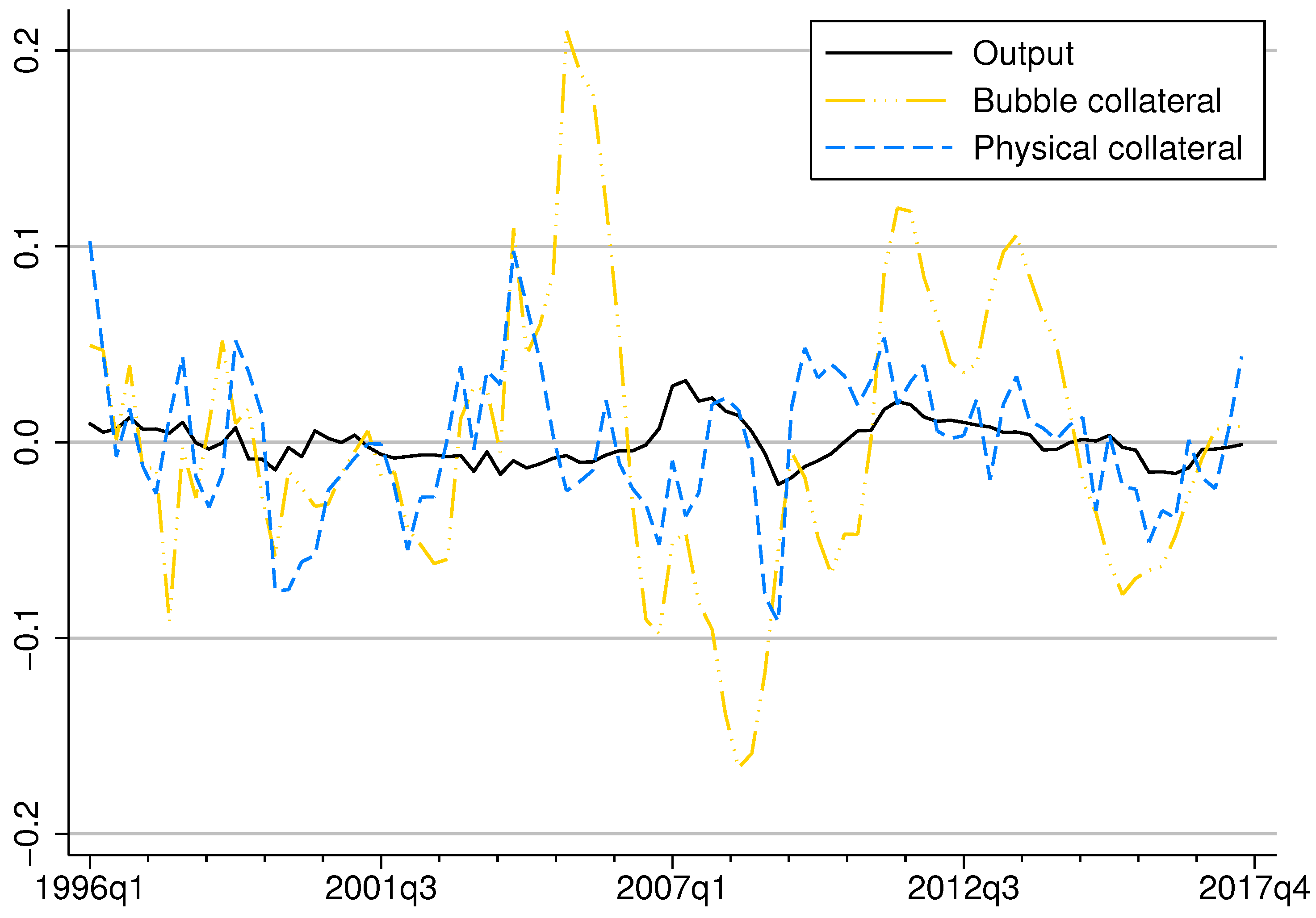
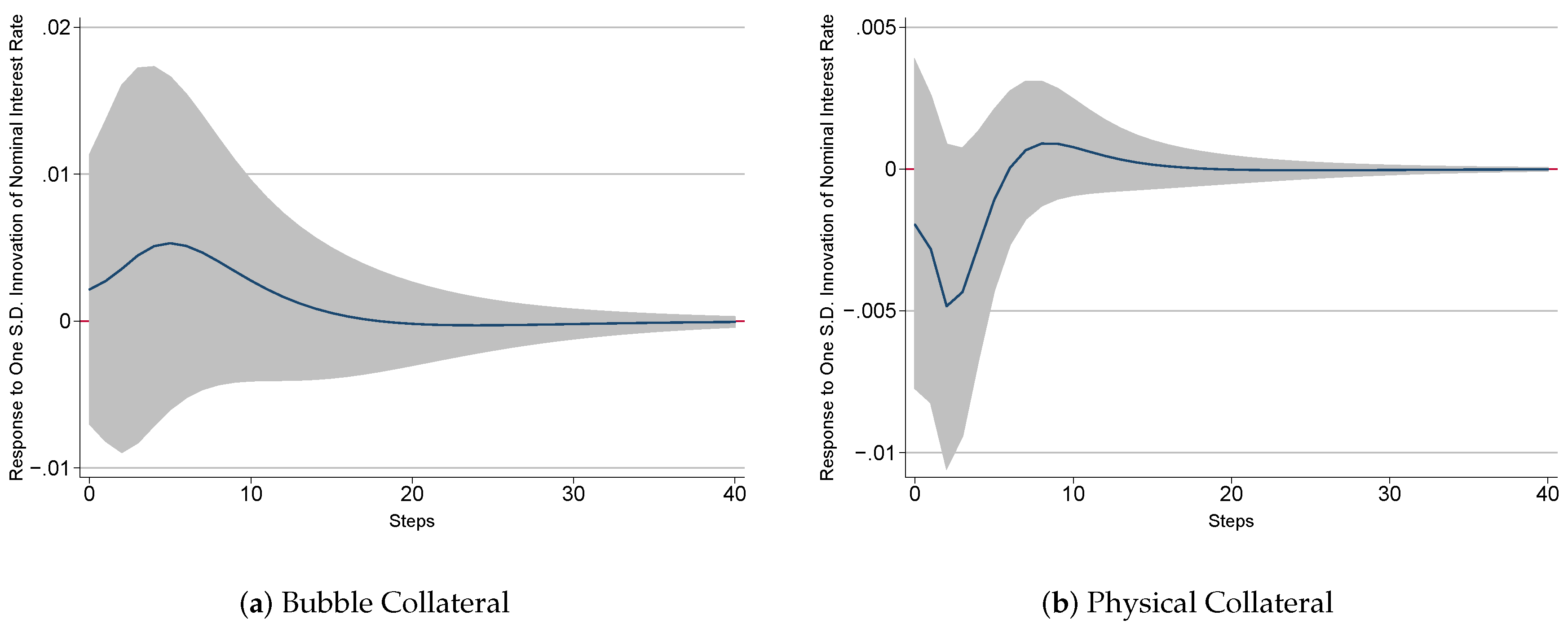
In a first step, in order to provide a comprehensive overview of the contradiction between persistently growing bubbles and elaborately designed regulatory methods, we collect the latest empirical evidence characterizing the salient features of collateral composition, which comprises inherently valueless bubble and classic physical capital. Quarterly China’s time series over the past years distinctly describe the strikingly high volatility of collateral bubble as well as its negative relationship with economic output. Apart from this, the VAR results show that, when the financial market is exposed to a standard interest rate shock, physical collateral suffers a direct and significant decline that does not last long, whereas its counterpart (bubble collateral) receives a continued moderate promotion. These findings substantiate our argument that rigid interest rate control depresses productivity and meanwhile encourages asset bubbles.

So as to explore the intrinsic mechanism of how these two collaterals evolve and interact with each other under certain collocation of monetary control and market pressure, this paper goes a step further to develop a generalized OLG model considering an imperfect market environment in the presence of limited commitment and insufficient liquidity. Under the constraint that investors can only receive a small amount of money from their pledged asset value, they have strong incentives to expand investment by off-balance sheet financing. Even worse, when commercial banks are required higher capital requirements or loan-to-deposit ratios (which are measured by the financial friction coefficient $\eta$ in our model), borrowers are in a more difficult position and rely more on unsustainable speculative bubbles to resolve the liquidity crisis.

In our specific model design, mathematical proofs justify the unique existence of a bubbly equilibrium, which implies that rational asset bubbles remain at a constant level under a reasonable interest rate. Moreover, the steady-state bubble size expands when the interest rate increases. After we calibrate the relevant parameters in accordance with existing literature and Chinese characteristics, we come up with numerical results further illustrating the collateral interactions and model dynamics behind the above manifestations. 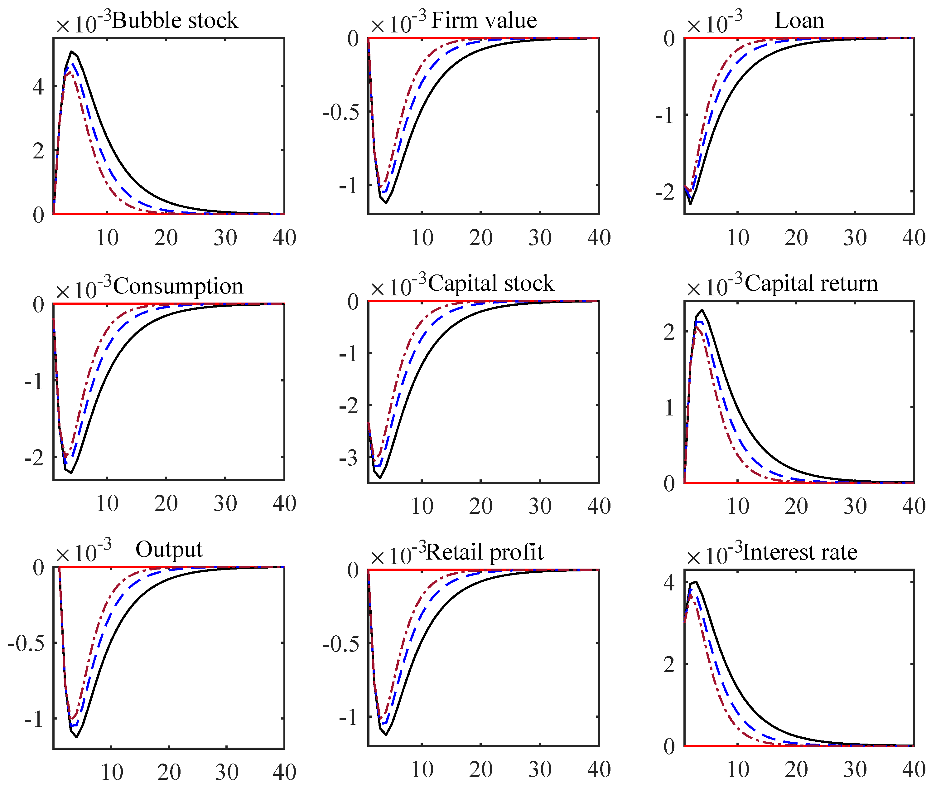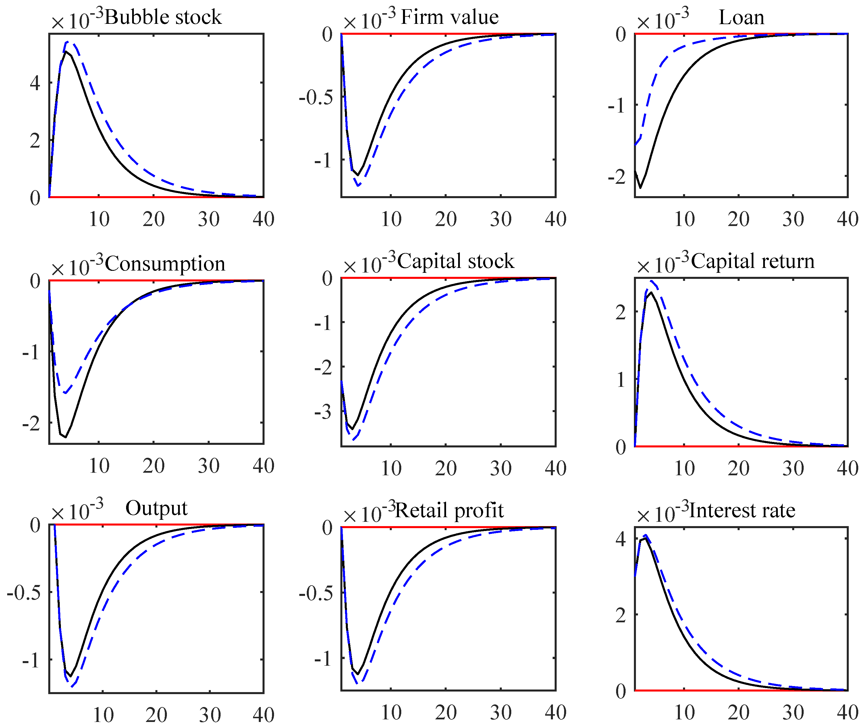From the comparative static analysis in Section 5.3, either the tightening of monetary control on R or the aggravation of credit condition on $\eta$ fosters bubble escalation and slows down economic growth at the same time. As the physical capital drops with contractionary measures, the pledgeable bubble asset instead rises up to cover the deficit in investor’s mortgage portfolio. Furthermore, from the impulse response analysis, the dynamic evolution in Section 5.4 indicates that an unanticipated interest rate rise indeed brings about an inflation effect on the bubble. In addition, deteriorated borrowing friction plays a prominent role as financial accelerator, magnifying the aforementioned expansionary effect to a higher level.

6.1. Policy Implications

Finally, we summarize some policy implications on the grounds of our research above.

First and foremost, the policy collocation of rigorous monetary control and drastic deleveraging campaign is not desirable allowing for non-ignorable frictions in financial markets. From a second thought, China has been fortunate enough to step in a continuous process of the credible market-oriented reform backed by aggressive macroeconomic stimulus and guaranteed political stability, for which its housing bubbles have thus far not provoked overturning consequences. Sadly, the situation is more grim. In particular, for those even less developed countries or economies with an imperfect capital market, in which asymmetric information and limited commitment give rise to the problem of credit rationing, insufficient investment caused by funds shortage forces productive enterprises to reduce production and even close down. In consequence, ordinary residents cannot but shift assets to a redundant housing market, finally leading to a tremendous amount of bubble and disaster-ridden household debt.

Our second implication is conditional. If and when the collateral constraint in a credit market is alleviated (due to, for example, more transparent information or less default possibility), the central bank is supposed to step up to fulfill its duty and apply an interest rate tool in a flexible way. This inference gives rise to a more profound conclusion: Given that the decision of financial regulators and supervisors on the tightness of credit constraint $\eta$ always involves a trade-off between the stabilization in asset markets and that in production markets (shown by the impulse response analysis in Section 5.4.3), it is preferable (provided all other conditions are equal) to salvage the social production at the first place, because at the very least, this decision leaves more policy space for monetary authorities to put their multiple instruments to good use.

In addition, a more conceptual element we should ponder over is the intrinsic attribute of real estate bubbles. In light of the inseparable relationship between market prices of land property and its additional values from future sale and original agriculture use, the broadly used income approach method might not be applicable for analyzing the real estate market, as is examined in detail by the authors in [48]. The fundamental value derived from the present value formula is not often indicative of the house property market, and the government need not overreact to the seemingly unexplained price premium within a controllable range. Other factors including transaction costs, the risk preference of home-buyers, and market expectations all form the real estate price with composite effects.

Last but not the least from the angle of credit transmission, the potential competence of monetary policy to surmount its major obstacle is expected to be restored if efficient macro prudential regulations prevent the formation of a positive feedback loop between bubbles and credit supply. Given the diversification and flexibility of their extended tool set as well as the rear position they are standing at, regulatory institutions have the desirability and feasibility to rupture the unsustainable relationship between bubble and credit, freeing the powerful effect of the interest rate policy.

6.2. Limitations and Future Research

With a view to maintaining the sound and durable real estate market, which is quite essential to improve people’s life quality, enable common residents to settle down peacefully, and ultimately realize a harmonious and stable society, a monetary policy that is too harsh is not recommended. A housing bubble associated with many derivative problems has become a troublesome issue in public debate since the subprime crisis, and this paper merely proceeds from the perspective of a collateral mechanism and provides fresh insight into the possibly appropriate policy measures. In a future study, we are interested in subdividing the households who hold real estate bubbles into age-specific heterogeneous groups. A more intricate design for more responsive young home-buyers is beyond the length of this article, but this could be a realistic and meaningful exploration for assessing the effects of demographic developments as well as an ageing population. In addition, another valuable research direction is to evaluate the environmental side effects of the twofold austerity campaign on price and on credit. Inspiring research has recently carefully and rigorously considered environmental and social characteristics: Using analytic hierarchy process (AHP) methodology on account of environmental factors such as urban clusters and rural grid cells, the authors in [49] propose a precise assessment of the sophisticated development trends in the Euro Area. They comprehensive studied the real estate market and made a convincing case of the potential necessity of a transition to modernized and newly constructed real estate portfolios. Similarly paying attention to the macroeconomic constraints on the operation and evolution of farmland assets, the authors in [50] emphasize the social and ecological values that have been greatly underestimated in the potential values of farmland in China. Under this circumstance, the deep relationships between house price, land reallocation, an ageing population, and residential structure are worth exploring. In the case of a dismal outlook on the housing market and an even worse financing environment, a rational real estate agency is very likely to sell off, leaving a bulk of abandoned and unfinished buildings. Dozens of uncompleted residential flats are extremely harmful to the sustainability of cultivated land and a balanced ecosystem and result in serious scarcity in nature and the environment.

References

1. Chen, K.; Higgins, P.; Waggoner, D.F.; Zha, T. Impacts of Monetary Stimulus on Credit Allocation and Macroeconomy: Evidence from China; Working Paper 22650; National Bureau of Economic Research: Cambridge, MA, USA, 2016. [Google Scholar] [CrossRef]
2. Iacoviello, M. House prices, borrowing constraints, and monetary policy in the business cycle. Am. Econ. Rev. 2005, 95, 739–764. [Google Scholar] [CrossRef]
3. Poterba, J.M.; Weil, D.N.; Shiller, R. House price dynamics: The role of tax policy and demography. Brook. Pap. Econ. Act. 1991, 1991, 143–203. [Google Scholar] [CrossRef]
4. Brunnermeier, M.K.; Julliard, C. Money illusion and housing frenzies. Rev. Financ. Stud. 2008, 21, 135–180. [Google Scholar] [CrossRef]
5. Genesove, D.; Han, L. Search and matching in the housing market. J. Urban Econ. 2012, 72, 31–45. [Google Scholar] [CrossRef]
6. Farhi, E.; Tirole, J. Bubbly liquidity. Rev. Financ. Stud. 2011, 79, 678–706. [Google Scholar] [CrossRef]
7. Martin, A.; Ventura, J. Economic growth with bubbles. Am. Econ. Rev. 2012, 102, 3033–3058. [Google Scholar] [CrossRef]
8. Martin, A.; Ventura, J. Managing credit bubbles. J. Eur. Econ. Assoc. 2016, 14, 753–789. [Google Scholar] [CrossRef]
9. Wang, P.; Wen, Y. Speculative bubbles and financial crises. Am. Econ. J. Macroecon. 2012, 4, 184–221. [Google Scholar] [CrossRef]
10. Miao, J.; Wang, P. Bubbles and Total Factor Productivity. Am. Econ. Rev. 2012, 102, 82–87. [Google Scholar] [CrossRef]
11. Miao, J.; Wang, P. Asset bubbles and credit constraints. Am. Econ. Rev. 2018, 108, 2590–2628. [Google Scholar] [CrossRef]
12. Galí, J. Monetary policy and rational asset price bubbles. Am. Econ. Rev. 2014, 104, 721–752. [Google Scholar] [CrossRef]
13. Tirole, J. Asset bubbles and overlapping generations. Econometrica 1985, 53, 1499–1528. [Google Scholar] [CrossRef]
14. Glaeser, E.L.; Gyourko, J.; Saiz, A. Housing Supply and Housing Bubbles; Working Paper 14193; National Bureau of Economic Research: Cambridge, MA, USA, 2008. [Google Scholar] [CrossRef]
15. Goodhart, C.A. Price stability and financial fragility. In Financial Stability in a Changing Environment; Palgrave Macmillan: London, UK, 1995; pp. 439–509. [Google Scholar] [CrossRef]
16. Kent, C.; Lowe, P. Asset-Price Bubbles and Monetary Policy; Reserve Bank of Australia: Sydney, Australia, 1997.
17. Cecchetti, S.G.; Genberg, H.; Lipsky, J.; Wadhwani, S. Asset Prices and Central Bank Policy; Geneva Reports on the World Economy; International Center for Monetary and Banking Studies: Geneva, Switzerland, 2000. [Google Scholar]
18. Pesce, M.A. Transmission Mechanisms for Monetary Policy in Emerging Market Economies: What Is New? Technical Report 35; Bank for International Settlements: Basel, Switzerland, 2008. [Google Scholar]
19. Chow, H.K.; Choy, K.M. Monetary policy and asset prices in a small open economy: A factor-augmented VAR analysis for Singapore. Ann. Financ. Econ. 2009, 5, 1–23. [Google Scholar] [CrossRef]
20. Smets, F.; Wouters, R. Shocks and frictions in US business cycles: A Bayesian DSGE approach. Am. Econ. Rev. 2007, 97, 586–606. [Google Scholar] [CrossRef]
21. Olsen, ∅. Integrating Financial Stability and Monetary Policy Analysis. Speech at the London School of Economics, 27 April 2015. Available online: https://www.norges-bank.no/ (accessed on 16 December 2018).
22. Gourio, F.; Kashyap, A.K.; Sim, J.W. The trade offs in Leaning Against the Wind. IMF Econ. Rev. 2018, 66, 70–115. [Google Scholar] [CrossRef]
23. Miao, J.; Shen, Z.; Wang, P. Monetary policy and rational asset price bubbles: Comment. Am. Econ. Rev. 2018. forthcoming. [Google Scholar]
24. Bernanke, B.S.; Gertler, M. Monetary Policy and Asset Price Volatility; Working Paper 7559; National Bureau of Economic Research: Cambridge, MA, USA, 2000. [Google Scholar] [CrossRef]
25. Bernanke, B.S.; Gertler, M. Should central banks respond to movements in asset prices? Am. Econ. Rev. 2001, 91, 253–257. [Google Scholar] [CrossRef]
26. Reinhart, V. Planning to Protect Against Asset Bubbles; Hunter, K., Pomerleano, Eds.; Asset Price Bubble; The MIT Press: Cambridge, MA, USA, 2003; pp. 553–560. [Google Scholar]
27. Mishkin, F.S. How should we respond to asset price bubbles? Financ. Stabil. Rev. 2008, 12, 65–74. [Google Scholar]
28. Conefrey, T.; Gerald, J.F. Managing housing bubbles in regional economies under EMU: Ireland and Spain. Natl. Inst. Econ. Rev. 2010, 211, 91–108. [Google Scholar] [CrossRef]
29. Farley, J.; Burke, M.; Flomenhoft, G.; Kelly, B.; Murray, D.F.; Posner, S.; Putnam, M.; Scanlan, A.; Witham, A. Monetary and fiscal policies for a finite planet. Sustainability 2013, 5, 2802–2826. [Google Scholar] [CrossRef]
30. Galí, J.; Gambetti, L. The effects of monetary policy on stock market bubbles: Some evidence. Am. Econ. J. Macroecon. 2015, 7, 233–257. [Google Scholar] [CrossRef]
31. Brunnermeier, M.; Schnabel, I. Bubbles and central banks: Historical perspectives. In Central Banks at a Crossroads: What Can We Learn from History? Number 10528; Cambridge University Press: Cambridge, UK, 2015. [Google Scholar]
32. Svensson, L.E. Cost-benefit analysis of Leaning Against the Wind. J. Monet. Econ. 2017, 90, 193–213. [Google Scholar] [CrossRef]
33. Juselius, M.; Borio, C.E.; Disyatat, P.; Drehmann, M. Monetary policy, the financial cycle and ultra-low interest rates. Int. J. Cent. Bank. 2017, 13, 55–89. [Google Scholar]
34. Fisher, I. The debt-deflation theory of great depressions. Econometrica 1933, 1, 337–357. [Google Scholar] [CrossRef]
35. Bernanke, B.S.; Gertler, M. Inside the black box: The credit channel of monetary policy transmission. J. Econ. Perspect. 1995, 9, 27–48. [Google Scholar] [CrossRef]
36. Kiyotaki, N.; Moore, J. Credit cycles. J. Polit. Econ. 1997, 105, 211–248. [Google Scholar] [CrossRef]
37. Carlstrom, C.T.; Fuerst, T.S. Agency costs, net worth, and business fluctuations: A computable general equilibrium analysis. Am. Econ. Rev. 1997, 87, 893–910. [Google Scholar] [CrossRef]
38. Bernanke, B.S.; Gertler, M.; Gilchrist, S. The financial accelerator in a quantitative business cycle framework. In Handbook of Macroeconomics; Elsevier: Amsterdam, The Netherlands, 1999; Volume 1, pp. 1341–1393. [Google Scholar] [CrossRef]
39. Kocherlakota, N. Bursting bubbles: Consequences and cures. In Proceedings of the Macroeconomic and Policy Challenges Following Financial Meltdowns Conference, Washington, DC, USA, 3 April 2009; Available online: https://www.imf.org/external/np/seminars/eng/2009/macro/index.htm/ (accessed on 10 December 2018).
40. Jermann, U.; Quadrini, V. Macroeconomic effects of financial shocks. Am. Econ. Rev. 2012, 102, 238–271. [Google Scholar] [CrossRef]
41. Miao, J.; Wang, P. Sectoral bubbles, misallocation, and endogenous growth. J. Math. Econ. 2014, 53, 153–163. [Google Scholar] [CrossRef] [Green Version]
42. Chen, K.; Ren, J.; Zha, T. The nexus of monetary policy and shadow banking in China. Am. Econ. Rev. 2018, in press. [Google Scholar] [CrossRef]
43. Allen, F.; Barlevy, G.; Gale, D. A theoretical model of Leaning Against the Wind; Federal Reserve Bank of Chicago Working Paper; Federal Reserve Bank of Chicago: Chicago, IL, USA, 2017. [Google Scholar]
44. Chang, C.; Chen, K.; Waggoner, D.F.; Zha, T. Trends and cycles in China’s macroeconomy. NBER Macroecon. Annu. 2016, 30, 1–84. [Google Scholar] [CrossRef]
45. Kaplan, G.; Violante, G.L.; Weidner, J. The wealthy hand-to-mouth. Brook. Pap. Econ. Act. 2014, 77–153. [Google Scholar] [CrossRef]
46. Lútkepohl, H. New Introduction to Multiple Time Series Analysis; Springer Science & Business Media: Berlin/Heidelberg, Germany, 2005. [Google Scholar]
47. Song, Z.; Storesletten, K.; Zilibotti, F. Growing like China. Am. Econ. Rev. 2011, 101, 196–233. [Google Scholar] [CrossRef]
48. Del Río, B.S.G.; Perez-Salas, J.; Cervello-Royo, R. Land value and returns on farmlands: An analysis by Spanish autonomous regions. Span. J. Agric. Res. 2012, 10, 271–280. [Google Scholar] [CrossRef]
49. Cervelló-Royo, R.; Guijarro, F.; Pfahler, T.; Preuss, M. An Analytic Hierarchy Process (AHP) framework for property valuation to identify the ideal 2050 portfolio mixes in EU-27 countries with shrinking populations. Qual. Quant. 2016, 50, 2313–2329. [Google Scholar] [CrossRef]
50. Hu, R.; Qiu, D.C.; Xie, D.T.; Wang, X.Y.; Zhang, L. Assessing the real value of farmland in China. J. Mt. Sci. 2014, 11, 1218–1230. [Google Scholar] [CrossRef]
Figure 1. Urban residential real estate development in China from 2008 to 2018. Data source: Survey and Research Center for China Household Finance (http://www.chfsdata.org/about.aspx).
Sustainability 10 04803 g001
Figure 2. Credit growth and evolution of shadow loan composition in China’s credit market between 2001Q4 and 2018Q2 (quarterly). Shadow loan ratio is the “end-of-quarter total lending in the shadow banking industry” divided by the “end-of-quarter total financial institution loans outstanding”. Real estate loans are “new loans to real estate” deflated by a CPI deflator. Data source: Center for Quantitative Economic Research (CQER), Federal Reserve Bank of Atlanta.
Sustainability 10 04803 g002
Figure 3. Time-series of collateral components and output (HP-filtered log quarterly values). “Output” is GDP by expenditure, “Bubble collateral” stands for residential investment, and “Physical Collateral” stands for gross capital formation. Data source: Center for Quantitative Economic Research (CQER), Federal Reserve Bank of Atlanta.
Sustainability 10 04803 g003
Figure 4. VAR stability test.
Sustainability 10 04803 g004
Figure 5. Dynamic responses of bubble and physical collaterals to a standard interest rate shock. Nominal interest rate is the 1-day Repo rate. “Bubble Collateral” and “Physical Collateral” are the same time series as in Table 1. Data source: Center for Quantitative Economic Research (CQER), Federal Reserve Bank of Atlanta.
Sustainability 10 04803 g005
Figure 6. Comparative statics of collateral composition. “Physical Collateral” denotes a firm value in our model, and the “Bubble Collateral” is the value of bubble stock accordingly.
Sustainability 10 04803 g006
Figure 7. Impulse responses to a contractionary monetary policy (MP) shock. Solid lines (benchmark): tight MP ( φ q = 0.8 ). Dashed lines: neutral MP ( φ q = 0 ). Dash-dotted lines: easing MP ( φ q = 0.8 ).
Sustainability 10 04803 g007
Figure 8. Impulse responses to a contractionary monetary policy shock. Solid lines (benchmark): moderate frictions ( η = 0.7 ). Dashed lines: severe frictions ( η = 0.5 ).
Sustainability 10 04803 g008