Identification of Vehicle-Pedestrian Collision Hotspots at the Micro-Level Using Network Kernel Density Estimation and Random Forests: A Case Study in Shanghai, China

Abstract

The improvement of pedestrian safety plays a crucial role in developing a safe and friendly walking environments, which can contribute to urban sustainability. A preliminary step in improving pedestrian safety is to identify hazardous road locations for pedestrians. This study proposes a framework for the identification of vehicle-pedestrian collision hot spots by integrating the information about both the likelihood of the occurrence of vehicle-pedestrian collisions and the potential for the reduction in vehicle-pedestrian crashes. First, a vehicle-pedestrian collision density surface was produced via network kernel density estimation. By assigning a threshold value, possible vehicle-pedestrian hot spots were identified. To obtain the potential for vehicle-pedestrian collision reduction, random forests was employed to model the density with a set of variables describing vehicle and pedestrian flows. The potential for crash reduction was then measured as the difference between the observed vehicle-pedestrian crash density and the prediction produced by the random forests models. The final hotspots were determined by excluding those with a crash reduction value of no more than zero. The method was applied to the identification of hazardous road locations for pedestrians in a district in Shanghai, China. The result indicates that the method is useful for decision-making support.

1. Introduction

People start and end most of their trips on foot in their daily lives. However, mainly due to the lack of awareness, pedestrians are often at high risk for death and injury. According to the World Health Organization [1], approximately 1.24 million traffic deaths occur annually on the world’s roads, of which about 22% involve pedestrians. As walking positively influences health and the environment, encouraging walking can help develop a sustainable community. Despite a shift from motorized to sustainable transport modes (such as walking and cycling) that have focused attention on pedestrian safety, there is still much room for improvement to ensure a safe walking environment for pedestrians.

A preliminary step to improve pedestrian safety is to identify hazardous road locations for pedestrians. This task plays a crucial role in safety countermeasure proposals and resource allocation. From a geography perspective, hazardous road locations are usually represented by clusters of traffic collisions. In the literature, extensive research has focused on the detection of traffic collision concentration at the micro levels [2,3,4,5,6,7,8,9,10,11,12]. The studies can be categorized into two types [13,14]. The first is the link-attribute class, where the road network is segmented into basic spatial units (BSUs) and treats the traffic collisions as attributes attached to the BSUs. The other is the event-based type, where individual traffic collision events represented by x and y coordinates in space are analyzed. In traffic collision analysis, kernel density estimation (KDE) is one of the most popular event-based approaches [15]. KDE has been widely applied to the identification of hazardous road locations. Although some researchers employed traditional planar KDE [16,17,18] that estimates density in two-dimensional space where traffic collisions are weighted based on the Euclidean distance, there has been a growing trend in applying network KDE (NKDE), which estimates density in a one-dimensional space where distance is calculated along the road network mainly because traffic collisions are a network-constrained phenomenon. For instance, Xie and Yan [5] developed a novel NKDE approach to estimate the density of network-constrained point events and applied it to the analysis of 2005 traffic crash data in the Bowling Green, Kentucky, USA area. The results indicate that the NKDE is more appropriate than standard planar KDE for density estimation of traffic collisions, since the latter is likely to overestimate the density values.

In the context of road safety, hazardous road locations are usually referred to as traffic collision “hotspots”, “blackspots”, ”sites with promise”, or “high risk locations”. A number of previous studies employed different methods to detect traffic collision hot spots based on traffic collision frequency and rate [19,20,21,22] aggregated by BSUs. Unlike spatial analysts who are interested in spatial analytical techniques for the detection of traffic collision clusters, traffic safety researchers are more concerned with the definition of hazardous road locations. Although using a simple ranking approach is the most convenient way of defining a traffic collision hotspot, it is thought that the method is naive and is likely to cause a large number of false positives. In handling this, previous studies have proposed other measures to define a hazardous (or unsafe) road locations. For instance, McGuigan [23,24] measured the “potential of accident reduction”, which was calculated as the difference between the observed and the expected crash count at a site given exposure. Mahalel et al. [25] suggested that locations that are selected for treatment should maximize the expected total reduction of traffic collisions. The premise of these studies is that only excess traffic collisions can be prevented by appropriate treatments [26]. However, most of these studies focused on vehicle-vehicle collisions and dealt with collision frequency. The method has not yet been applied to vehicle-pedestrian collision density.

As there is been no consensus on the best method of detecting hazardous road locations, this study proposes an integrated micro-level method that incorporates both traffic crash intensity and the potential for reduction to identify vehicle-pedestrian collision hot spots. The reasons for developing the method are twofold. Firstly, there is a growing trend among nations worldwide to set a “zero” tolerance vision in terms of fatalities to protect road users. To realize the ambitious target of zero road fatalities and serious injuries on roads, researchers and engineers should be concerned with locations where traffic collisions happen frequently. Secondly, in safety practice, resources are usually insufficient for treating every hazardous road location. Policy-makers may not be interested in traffic crash clusters that only result from high traffic volume. They may, instead, like to know hazardous road locations that produce the maximum reduction in traffic deaths and injuries when appropriately treated. In this light, we attempted to develop a framework to integrate both crash density and reduction potential information sources for decision-making support for pedestrian safety.

The following section first introduces the steps for identifying vehicle-pedestrian hot spots, with emphasis on models we used to analyse vehicle-pedestrian collisions. The study area and data are introduced in Section 3, and the results are presented and discussed in Section 4, followed by conclusions and further research directions in Section 5.

2. Method

The proposed framework for the identification of vehicle-pedestrian collision hot spots involves three steps: producing a vehicle-pedestrian collision density surface, measuring the potential for vehicle-pedestrian collision reduction, and identifying the vehicle-pedestrian collision hot spots. This section introduces the models and approaches employed in each step.

2.1. Generation of Vehicle-Pedestrian Collision Density Surface

The NKDE method was used for detecting the vehicle-pedestrian collision hot spots by following the approach in Xie and Yan [5] and Loo et al. [12]. First, by analogy with standard planar KDE, where the entire two-dimensional space is divided into regular grids, the roads were divided into BSUs in equal intervals to ensure regularly spaced locations along a network for density estimation [5]. Next, the center points of BSUs were obtained as reference points. For each reference point (RP), the density estimate, f_(i), is calculated by:

$$f_{\left(i\right)}=\frac{1}{Nb}{\displaystyle \sum }_{j=1}^{N}Kern(\frac{d_{ij}}{b})$$

(1)

where b is the bandwidth, d_ij is the network distance between reference point i and vehicle-pedestrian traffic collision j, and Kern(.) is a kernel function that measures the distance decay effect, such as Uniform, Triangle, Quartic, Triweight, and Gaussian [27]. In this study, the length of BSU was set as 200 m, and the Quartic function was chosen as the kernel function, which is determined by:

$$Kern(\frac{d_{ij}}{b})=\{\begin{array}{cc}\frac{15}{16}{(1-\frac{{d_{ij}}^2}{b^2})}^2\hfill & if0<\frac{d_{ij}}{b}\le 1\hfill \\ 0\hfill & otherwise;\hfill \end{array}$$

(2)

Although the BSU length and the choice of kernel function may have limited influence on the results, the selection of bandwidth has significant impacts on the resultant density surface [4,5,12]. A small bandwidth may produce a sharp density pattern and may result in a large number of tiny isolated individual clusters, and a broad bandwidth produces smooth density surface where hazardous road locations are likely to be mixed with safe neighboring locations. In this research, the bandwidth was chosen as 250 m—an intermediate value—to ensure an appropriate density surface.

2.2. Calculation of Potential of Vehicle-Pedestrian Collision Reduction

The potential for vehicle-pedestrian collision reduction was measured as the difference between the observed and the estimated crash density values. The former is obtained using Equations (1) and (2), the latter can be calculated by modelling the vehicle-pedestrian crash density with variables that describe not only vehicle volume but also pedestrian flow. Although traditional statistical models have been widely used in traffic collision modelling [28,29,30], applying machine learning methods [31,32,33] has become a growing trend. A typical example is Chang [31] who analysed freeway collisions with neural network (NN) approaches and found that NN models had better predictive performance because of their exceptional ability in approximating the complicated nonlinearity. However, NNs have limited ability to illustrate the influence of risk factors due to the “black-box” drawback and are likely to cause a severe over-fitting problem. To balance the explanatory ability of risk factors and the accuracy of traffic collision prediction, we employed the random forest (RF) method [34,35] for modeling traffic collisions, because the technique is relatively robust to outliers and can evaluate the relative importance of potential predictors [36]. The RF technique is being increasingly applied to many research fields such as classification of land cover [37], identification of fire occurrence [38], mapping of oil spill [39], detection of gold potential [40], and diagnosis of tree health [41]; however, it has rarely been applied to the modeling of traffic collision density.

RF was first proposed by Breiman [35]. The technique relies on the “bagging” method that constructs each tree independently by using a bootstrap sample of the dataset [42]. A random forest consists of many trees, each of which is generated by drawing bootstrap samples from the original dataset, with “out-of-bag” (OOB) data for validation. Unlike in standard trees where each node is split using the best among all predictors, in a random forest, each node is split by randomly sampling a subset of predictors and choosing the best split among those variables [34]. The outcome of the RFs is determined by averaging the predictions of all the trees [35]. The importance of each predictor can be estimated by examining the increase in prediction error when permuting the OOB data for that variable and leaving all others unchanged. Two commonly used measures in RFs for assessing variable importance are the mean decrease in accuracy and the decrease in node impurity. As the former indicator is considered a more reliable measure [43], it was used for measuring the variable importance in this study.

This study employed the Sci-Kit Learn (SKlearn, The French Institute for Research in Computer Science and Automation, Rocquencourt, France) toolkit [44] that provides machine learning tools in Python for data mining and data analysis. In SKlearn, the RandomForestRegressor tool was used for implementing the RF algorithm. It contains several parameters that allow users to specify modifications for optimizing the model, including n estimators (the number of decision trees), criterion (the method to measure the quality of a split), max_depth (the maximum depth of a decision tree), and min_samples_split (the minimum sample size in a split). SKlearn also provides functions that enable users to measure the prediction accuracy of the model, such as cross_val_score mean_squared_error, mean_absolute_error, and r2_score, which compute the values of mean squared error, mean absolute error, and R², respectively. The function feature_importances is used for measuring the importance of each variable.

Although independent validation samples are not necessary for RF, they allow the assessment of the generalization capability of the method [38,45]. In this light, the dataset was randomly divided into two parts: 70% for calibration and 30% for validation. The procedure was repeated n times, resulting in n sub-samples. The final predicted density value was determined by averaging predictions from RF models based on n sub-samples. The potential for vehicle-pedestrian collision reduction was then obtained by calculating the difference between the observed vehicle-pedestrian collision density and the final prediction. In this study, n was set to five.

2.3. Identification of Vehicle-Pedestrian Collision Hot Spots

The potential vehicle-pedestrian collision hot spots were first detected by setting a threshold value for crash density. For each of these locations, the potential for vehicle-pedestrian collision reduction was examined. If the value was no more than zero, the site was treated as a false positive and was excluded from the hot spots. The final hazardous road locations for pedestrians only included those with the potential for collision reduction above zero. Following Harirforoush and Bellalite [4], the threshold value was set to three standard deviations from the mean value in this research.

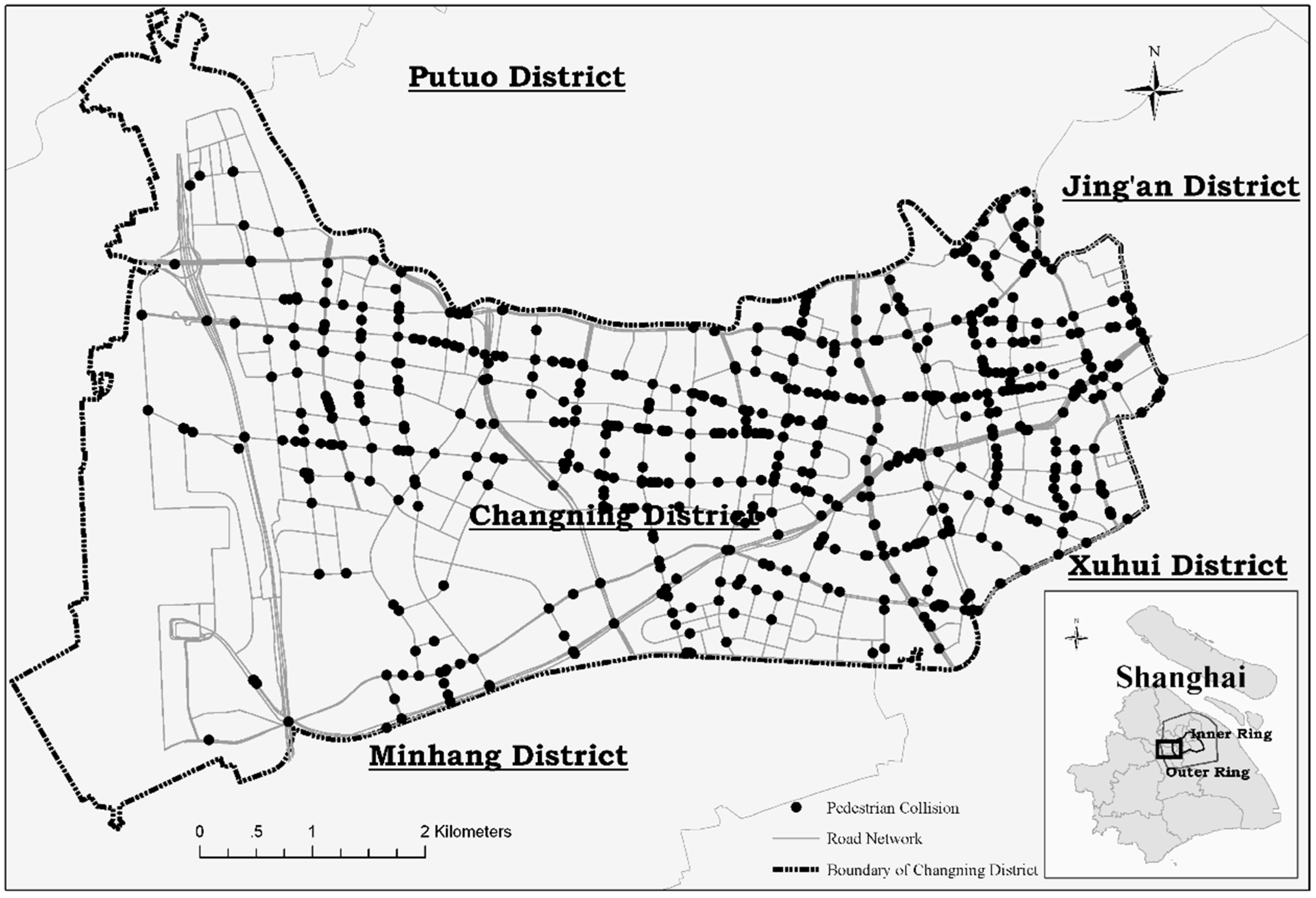
3. Study Area and Data

We analysed vehicle-pedestrian collisions occurring in 2015 in Changning District, which is located in the urban core of Shanghai, China. The vehicle-pedestrian collision data were collected from the Shanghai 110 Calling Center. The total length of arterial, secondary, and branch roads in this district is about 295 km. In 2015, 1200 vehicle-pedestrian collisions occurred in the district. Figure 1 shows the spatial distribution of vehicle-pedestrian crashes in the study area. In traffic safety research, the analysis is usually conducted based on crash data observed for 3- to 5-year periods; however, this study only used a dataset for one year. The reasons for this are twofold. First, given the length of the road network in the study area, 1200 vehicle-pedestrian collisions are able to depict overall pedestrian safety. It is not necessary to pool 3- or 5-year datasets to ensure the representativeness of the events. Second, since the late 2000s, the Shanghai Police has enforced a set of safety rules , which may result in significant yearly variation in safety performance.

As mentioned earlier, to determine the potential for vehicle-pedestrian collision reduction, the vehicle-pedestrian collision density should be modeled by RF with variables that describe both vehicle and pedestrian volume. Because it is challenging and extremely costly to collect detailed information on the vehicle and pedestrian volume along roads, we employed proxy variables that may reflect the spatial variation in flows.

One crucial variable delineating traffic volume is the Global Positioning System (GPS) data extracted from GPS-equipped taxis. Such on-vehicle GPS data have been widely used in various fields such as urban traffic surveillance, trip pattern identification, city structure recognition, and traffic safety on arterial roads [46,47,48,49], but have not been applied to the modeling of vehicle-pedestrian collision density. The data were collected from nearly 13,000 GPS-equipped taxis from Shanghai Qiangsheng Holding Co., Ltd. (Shanghai, China) The Qiangsheng family owns about 25% of the total number of taxis, which represents 4–7% of the vehicle population in Shanghai [49]. The Qiangsheng taxi GPS tracking point database contains information including vehicle identification (ID), time, speed, and longitude and latitude recorded by GPS receivers on the vehicles about every 10 s. With locational information, GPS points were plotted onto a map. A map-matching process was then conducted to ensure that the tracking points were assigned to appropriate roads [50]. For each reference point, the number of taxis that passed was calculated. In this study, taxi GPS tracking data 1–7 March 2016 were used for the calculation. The average daily taxi flow was introduced as the vehicle exposure variable for the vehicle-pedestrian collision density prediction models. One crucial issue is that the travel patterns and characteristics of taxicabs may differ from that of general traffic. A typical problem is that unoccupied taxis tend to cluster in some specific types of places such as shopping malls and metro stations. Including unoccupied taxis may cause overestimation of traffic flow in these locations. As trajectories of occupied taxis are more likely to reflect travel demands and hence the variation in real traffic, only taxis with passengers were included in the sample.

In addition to vehicle flow, the pedestrian volume plays a crucial role in vehicle-pedestrian safety models. In the absence of detailed pedestrian flow data, we employed a set of variables that comprehensively reflect characteristics of pedestrian flow. As different uses of land may suggest diverse activities of human beings, which influence different features of pedestrian flow [51,52,53], we employed land use data to reflect the spatial variation in pedestrian exposure. Point of Interest (POI) data that could be used to further segment the activities were also introduced into the RF model to incorporate more detailed features on pedestrian flow. In this research, land use data were derived from Landsat (National Aeronautics and Space Administration, Washington, DC, US) images from 2014 with a spatial resolution of 30 m. POIs were collected from Baidu, Inc. (Beijing, China) in 2014. The company provides application programming interfaces whereby users are allowed to develop programs for collecting POI information from Baidu Map. As some land use and POI variables are highly correlated, not all types of land use and POIs were integrated into the prediction models.

Table 1. Description of variables in the vehicle-pedestrian collision density models.

Variable Name	Data Source	Description
NoMetro	Point of Interest	No. of metro stations within 500 m of a Reference Point
NoBusStop	POI	No. of bus stops within 500 m of a RP
NoGov	POI	No. of government institutions within 500 m of a RP
NoBank	POI	No. of banking service facilities within 500 m of a RP
NoComBld	POI	No. of commercial buildings within 500 m of a RP
NoRetShp	POI	No. of retail shops within 500 m of a RP
NoMedi	POI	No. of medical service facilities within 500 m of a RP
NoEdu	POI	No. of educational institutions within 500 m of a RP
NoComp	POI	No. of companies within 500 m of a RP
NoPlaza	POI	No. of pedestrian plazas within 500 m of a RP
NoResi	POI	No. of residence places within 500 m of a RP
NoRest	POI	No. of restaurants within 500 m of a RP
AreaResi	Land use	Residential area (sq. m) within 500 m of a RP
AreaIndu	Land use	Industrial area (sq. m) within 500 m of a RP
AreaCom	Land use	Commercial area (sq. m) within 500 m of a RP
NoTaxi	Global Positioning System tracking point	No. of taxies that pass a RP

describes the variables that were finally introduced in the vehicle-pedestrian collision density models. The result of the collinearity test for these variables was 3.4, reflecting little collinearity.

Due to data availability, we used the 2015 vehicle-pedestrian collision data, taxi GPS data from 2016, and land use and POI datasets from 2014. Since Changning District is located in the urban area of Shanghai where the features of the built environment did not vary significantly from 2014 to 2016, it was reasonable to conduct analysis based on datasets collected from different years during this period.

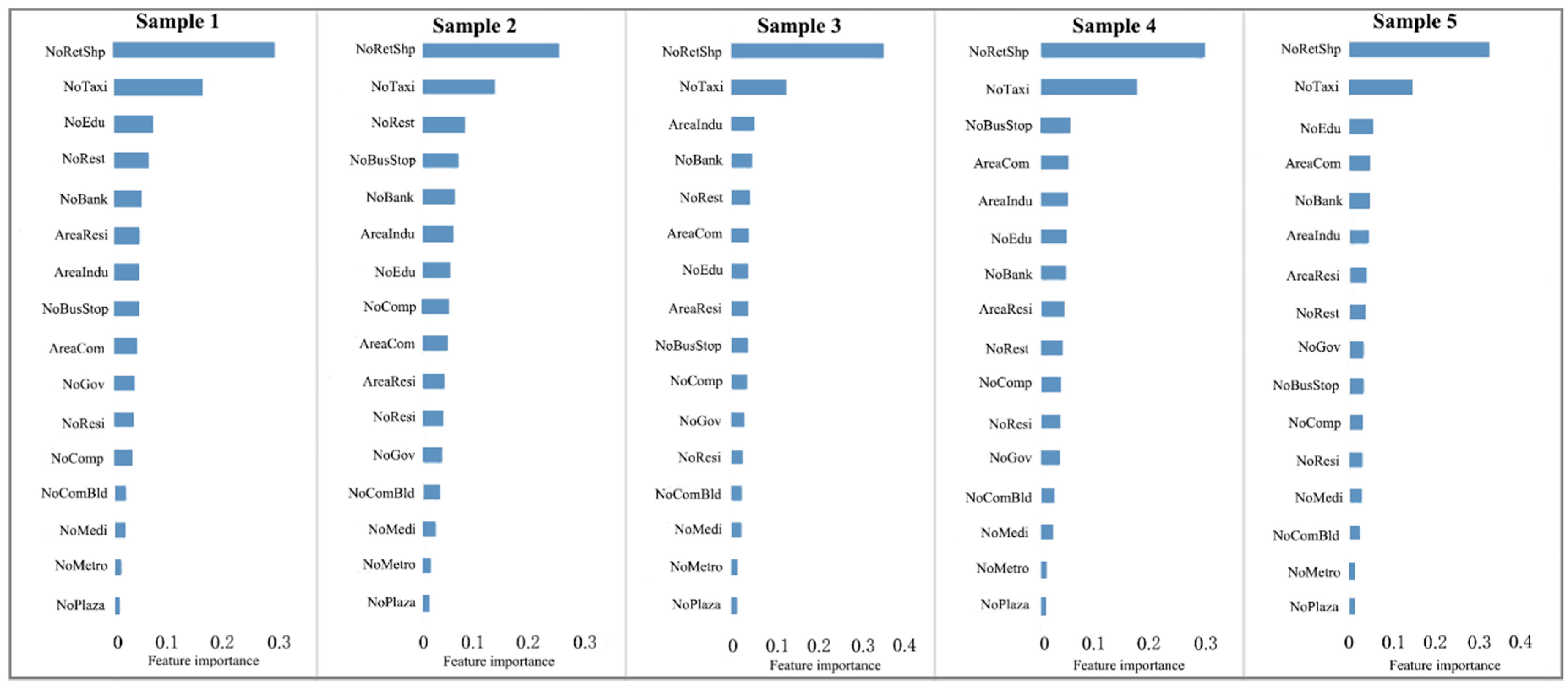
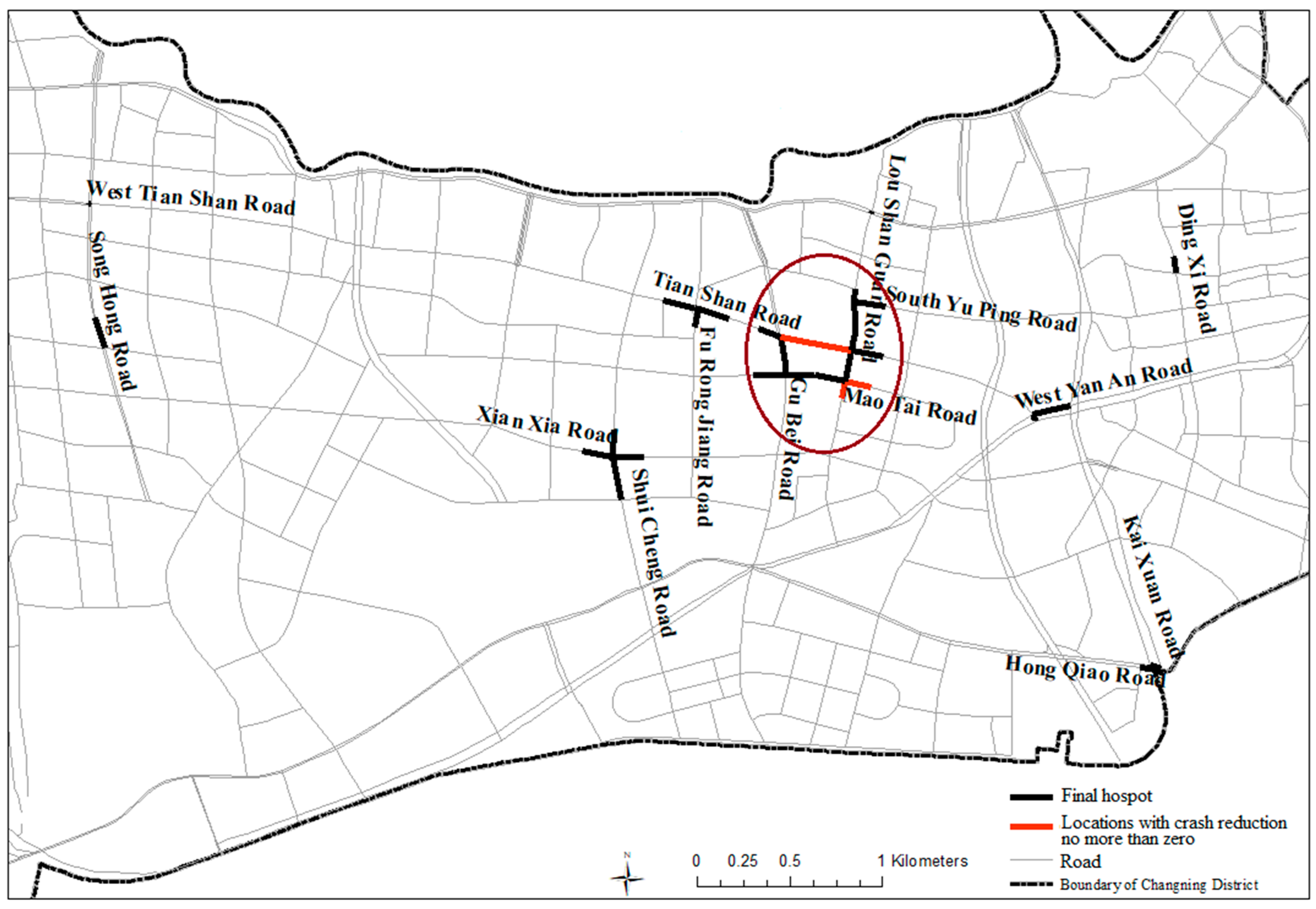
4. Result and Discussion

There were 1723 BSUs after the segmentation process. Following Equations (1) and (2), the vehicle-pedestrian density surface was produced, and the mean and standard deviation values were 0.008 and 0.01, respectively. The threshold value for identifying potential vehicle-pedestrian collision hot spots was computed as 0.038, which resulted in 35 possible hazardous road locations for pedestrians.

The RF models were established using GridsearchCV in SKlearn for parameter adjustment. In this study, n_estimator, max_depth, and min_samples_split were set from 100 to 200, 2 to 30, and 2 to 20, respectively. The values of the mean cross-validation score, mean squared error, median absolute error, and R² for each sample are presented in

Table 2. Results of Random Forest (RF) models.

	Mean Cross-Validation Score	Mean Squared Error	Median Absolute Error	R2
Sample 1	0.61 (±0.12)	0.0040	0.0247	0.6191
Sample 2	0.59 (±0.09)	0.0037	0.0260	0.6868
Sample 3	0.59 (±0.12)	0.0039	0.0260	0.6351
Sample 4	0.56 (±0.20)	0.0048	0.0278	0.6457
Sample 5	0.58 (±0.07)	0.0032	0.0292	0.6624

. Regardless of the sample, the value of R² was above 0.60. The mean cross validation scores were about 0.60 and slightly fluctuated, which suggests that the results were relatively stable. The values of the mean squared error and median absolute error were small. All these indicators reflect that the RF models could explain, to a large extent, the variation in vehicle-pedestrian collision density when vehicle and pedestrian exposure variables were considered. The result also indicates that the occurrence of vehicle-pedestrian collisions may result from exposures (vehicle and pedestrian flows in this study), as well as from some risk factors that require further investigation for treatment. This is the reason why it was essential to consider the potential for collision reduction.

As mentioned before, the RF technique has strength in dealing with the complicated nonlinearity relationship between the vehicle (or pedestrian) flow and occurrence of vehicle-pedestrian collisions. Although it may have some black-box problems, RF is capable of providing importance of variables (also called “features” in RF). Figure 2 shows the value of the importance for each variable with different samples. Although the importance of each variable varied in different samples, two variables—the number of retail shops and the taxi flow—ranked as the top two regardless of which sample was used. The mean feature importance of the two variables among the five samples was 0.3 and 0.15, respectively, indicating their ability to predict the occurrence of vehicle-pedestrian collisions. As mentioned before, previous studies have already investigated the relationship between land use characteristics and the occurrence of traffic crashes involving pedestrians [30,51], and it was found that vehicle-pedestrian collisions were more likely to happen in commercial areas. In this study, the commercial land was further segmented into different types of places such as retail shops and restaurants. The average importance value of the number of retail shops ranked in first place (see NoRetShp in Figure 2); the value of the restaurant count ranged from 0.04 to 0.08. This may have occurred because different kinds of activities may produce diverse types of pedestrian flow, thus significantly influencing the occurrence of vehicle-pedestrian collisions. The findings suggest that introducing POIs into the vehicle-pedestrian crash prediction models is desirable.

The final predicted vehicle-pedestrian collision density was produced by averaging the predictions of five samples, and the potential of collision reduction was then calculated by subtracting the prediction from the observation of vehicle-pedestrian collision density. Altogether, there were 634 BSUs with collision reduction potential. By comparing the resultant locations with those detected by merely setting the density threshold value, 4 of 35 potential hot spots were excluded. Figure 3 shows the spatial distribution of hot spots that were finally determined as hazards for pedestrians (see solid black lines in Figure 3), as well as locations with no crash reduction potential (see solid red lines in Figure 3). It can be observed from the figure that hot spots were also clustered, resulting in several hot zones for pedestrians. Some notable hot spots in this district (see the ellipse in Figure 3) were located in Tian Shan Road, Gu Bei Road, Mao Tai Road, Lou Shan Guan Road, and South Yu Ping Road. If the potential for vehicle-pedestrian collision reduction was not considered, the length of the roads that required further examination, including those colored in both black and red in the figure, was 2.7 km in total. When the proposed integrated method was applied, only 1.8 km of road segments were identified as hazardous. This allows engineers and policy-makers to focus their efforts on locations where there might be a higher likelihood of improving pedestrian safety.

Notably, in the absence of detailed vehicle and pedestrian exposure information at the micro level, we employed three variables—taxi flow, land use, and POI data—to reflect the variation in traffic and pedestrian characteristics across the study area by following previous studies on the relationship between the vehicle volume (or pedestrian flow) and taxi flow (or land use characteristics) [52,53,54]. Although the focus of this research was not the validation of the three variables as proxies of vehicle and pedestrian flow, the way in which vehicle and pedestrian exposure can be measured has always been an area of interest in road safety research [30]. With more experiments on the feasibility of proxy variables being performed in future, better tools can be developed to increase the precision of the estimation, and the proposed method in this research could be further improved.

5. Conclusions

The improvement in pedestrian safety plays a crucial role in developing a safe and friendly walking environment to help ensure urban sustainability. Given the importance of hot spot detection in safety management, we proposed a framework for the identification of hazardous road locations for pedestrians by integrating the likelihood of the occurrence of vehicle-pedestrian collisions and the potential for the reduction in traffic collisions involving vehicles and pedestrians. The research is of significance by not only theoretically enriching the methodology of hotspot identification but also practically providing useful information for policy-makers to propose countermeasures for pedestrian safety.

The method through which traffic and pedestrian exposures are measured by taxi trajectories, land use, and POI variables has not been fully explored. As a further step, research efforts may be dedicated to additional validation experiments. We used the proposed framework to identify the vehicle-pedestrian crash hot spots in only one period. If more vehicle-pedestrian collision data in other periods are available, the usefulness of the framework can be further examined. As the identification of hazardous road locations is the first step in safety improvement programs, future studies should investigate risk factors and the treatment of hot spots.

References

1. WHO. Global Status Report on Road Safety 2015; World Health Organization: Geneva, Switzerland, 2015. [Google Scholar]
2. Loo, B.P.Y.; Yao, S. The Identification of Traffic Crash Hot Zones under the Link-Attribute and Event-Based Approaches in a Network-Constrained Environment. Comput. Environ. Urban Syst. 2013, 41, 249–261. [Google Scholar] [CrossRef]
3. Yamada, I.; Thill, J.C. Local Indicators of Network-Constrained Clusters in Spatial Patterns Represented by a Link Attribute. Ann. Assoc. Am. Geogr. 2010, 100, 269–285. [Google Scholar] [CrossRef]
4. Harirforoush, H.; Bellalite, L. A New Integrated GIS-Based Analysis to Detect Hotspots: A Case Study of the City of Sherbrooke. Accid. Anal. Prev. 2016, in press. [Google Scholar] [CrossRef] [PubMed]
5. Xie, Z.; Yan, J. Kernel Density Estimation of Traffic Accidents in a Network Space. Comput. Environ. Urban Syst. 2008, 32, 396–406. [Google Scholar] [CrossRef]
6. Xie, Z.; Yan, J. Detecting Traffic Accident Clusters with Network Kernel Density Estimation and Local Spatial Statistics: An Integrated Approach. J. Transp. Geogr. 2013, 31, 64–71. [Google Scholar] [CrossRef]
7. Cheng, W.; Washington, S.P. Experimental Evaluation of Hotspot Identification Methods. Accid. Anal. Prev. 2005, 37, 870–881. [Google Scholar] [CrossRef] [PubMed]
8. Long, T.T.; Somenahalli, S.V.C. Using GIS to Identify Pedestrian-Vehicle Crash Hot Spots and Unsafe Bus Stops. J. Public Trans. 2011, 14, 99–114. [Google Scholar] [CrossRef] [Green Version]
9. Hao, Y.; Liu, P.; Chen, J.; Wang, H. Comparative Analysis of the Spatial Analysis Methods for Hotspot Identification. Accid. Anal. Prev. 2014, 66, 80–88. [Google Scholar] [CrossRef]
10. Nie, K.; Wang, Z.; Du, Q.; Ren, F.; Tian, Q. A Network-Constrained Integrated Method for Detecting Spatial Cluster and Risk Location of Traffic Crash: A Case Study from Wuhan, China. Sustainability 2015, 7, 2662–2677. [Google Scholar] [CrossRef] [Green Version]
11. Naji, H.A.H.; Xue, Q.; Lyu, N.; Wu, C.; Zheng, K. Evaluating the Driving Risk of near-Crash Events Using a Mixed-Ordered Logit Model. Sustainability 2018, 10, 2868. [Google Scholar] [CrossRef]
12. Loo, B.P.; Yao, S.; Wu, J. Spatial Point Analysis of Road Crashes in Shanghai: A GIS-Based Network Kernel Density Method. In Proceedings of the 19th International Conference on Geoinformatics, Shanghai, China, 24–26 June 2011. [Google Scholar]
13. Yamada, I.; Thill, J.C. Local Indicators of Network-Constrained Clusters in Spatial Point Patterns. Geogr. Anal. 2007, 39, 268–292. [Google Scholar] [CrossRef] [Green Version]
14. Yao, S.; Loo, B.P.; Yang, B.Z. Traffic Collisions in Space: Four Decades of Advancement in Applied GIS. Ann. GIS 2016, 22, 1–14. [Google Scholar] [CrossRef]
15. Silverman, B.W. Density Estimation for Statistics and Data Analysis; Chapman & Hall/CRC Press: Boca Raton, FL, USA, 1986. [Google Scholar]
16. Flahaut, B.; Mouchart, M.; Martin, E.S.; Thomas, I. The Local Spatial Autocorrelation and the Kernel Method for Identifying Black Zones: A Comparative Approach. Accid. Anal. Prev. 2003, 35, 991–1004. [Google Scholar] [CrossRef]
17. Erdogan, S.; Yilmaz, I.; Baybura, T.; Gullu, M. Geographical Information Systems Aided Traffic Accident Analysis System Case Study: City of Afyonkarahisar. Accid. Anal. Prev. 2008, 40, 174–181. [Google Scholar] [CrossRef] [PubMed]
18. Krisp, J.M.; Durot, S. Segmentation of Lines Based on Point Densities—An Optimisation of Wildlife Warning Sign Placement in Southern Finland. Accid. Anal. Prev. 2007, 39, 38–46. [Google Scholar] [CrossRef] [PubMed]
19. Deacon, J.A.; Charles, V.Z.; Deen, R.C. Identification of Hazardous Rural Highway Locations. Transp. Res. Rec. 1974, 410. [Google Scholar] [CrossRef]
20. Norden, M.; Orlansky, J.; Jacobs, H. Application of Statistical Quality-Control Techniques to Analysis of Highway-Accident Data. Highw. Res. Board Bull. 1956, 117, 17–31. [Google Scholar]
21. Morin, D.A. Application of Statistical Concepts to Accident Data. Highw. Res. Rec. 1967, 188, 72–79. [Google Scholar]
22. Stokes, R.; Mutabazi, M. Rate-Quality Control Method of Identifying Hazardous Road Locations. Transp. Res. Rec. 1996, 1542, 44–48. [Google Scholar] [CrossRef]
23. McGuigan, D.R.D. The Use of Relationships between Road Accidents and Traffic Flow in “Black-Spot” Identification. Traffic Eng. Control 1981, 22, 448–453. [Google Scholar]
24. McGuigan, D.R.D. Non-Junction Accident Rates and Their Use In ‘black-Spot’ Identification. Traffic Eng. Control 1982, 23, 60–65. [Google Scholar]
25. Mahalel, D.; Hakkert, A.S.; Prashker, J.N. A System for the Allocation of Safety Resources on a Road Network. Accid. Anal. Prev. 1982, 14, 45–56. [Google Scholar] [CrossRef]
26. Cheng, W.; Washington, S. New Criteria for Evaluating Methods of Identifying Hot Spots. Transp. Res. Rec. 2008, 2083, 76–85. [Google Scholar] [CrossRef] [Green Version]
27. Waller, L.A.; Gotway, C.A. Applied Spatial Statistics for Public Health Data; Wiley-Interscience: Hoboken, NJ, USA, 2004. [Google Scholar]
28. Huang, H.; Hong, C.C. Modeling Road Traffic Crashes with Zero-Inflation and Site-Specific Random Effects. Stat. Methods Appl. 2010, 19, 445–462. [Google Scholar] [CrossRef]
29. Anastasopoulos, P.C.; Mannering, F.L. A Note on Modeling Vehicle Accident Frequencies with Random-Parameters Count Models. Accid. Anal. Prev. 2009, 41, 153–159. [Google Scholar] [CrossRef] [PubMed]
30. Yao, S.; Loo, B.P.Y.; Lam, W.W.Y. Measures of Activity-Based Pedestrian Exposure to the Risk of Vehicle-Pedestrian Collisions: Space-Time Path Vs. Potential Path Tree Methods. Accid. Anal. Prev. 2015, 75, 320–332. [Google Scholar] [CrossRef] [PubMed]
31. Chang, L.Y. Analysis of Freeway Accident Frequencies: Negative Binomial Regression Versus Artificial Neural Network. Saf. Sci. 2005, 43, 541–557. [Google Scholar] [CrossRef]
32. Xie, Y.; Lord, D.; Zhang, Y. Predicting Motor Vehicle Collisions Using Bayesian Neural Network Models: An Empirical Analysis. Accid. Anal. Prev. 2007, 39, 922–933. [Google Scholar] [CrossRef]
33. Zeng, Q.; Huang, H.; Xin, P.; Wong, S.C.; Gao, M. Rule Extraction from an Optimized Neural Network for Traffic Crash Frequency Modeling. Accid. Anal. Prev. 2016, 97, 87–95. [Google Scholar] [CrossRef]
34. Liaw, A.; Wiener, M. Classification and Regression by Randomforest. R News 2002, 2, 18–22. [Google Scholar]
35. Breiman, L. Random Forests. Mach. Learn. 2001, 45, 5–32. [Google Scholar] [CrossRef] [Green Version]
36. Gromping, U. Variable Importance Assessment in Regression: Linear Regression Versus Random Forest. Am. Stat. 2009, 63, 308–319. [Google Scholar] [CrossRef]
37. Haas, J.; Ban, Y. Urban Growth and Environmental Impacts in Jing-Jin-Ji, the Yangtze, River Delta and the Pearl River Delta. Int. J. Appl. Earth Obs. Geoinf. 2014, 30, 42–55. [Google Scholar] [CrossRef]
38. Oliveira, S.; Oehler, F.; San-Miguel-Ayanz, J.; Camia, A.; Pereira, J.M.C. Modeling Spatial Patterns of Fire Occurrence in Mediterranean Europe Using Multiple Regression and Random Forest. For. Ecol. Manag. 2012, 275, 117–129. [Google Scholar] [CrossRef]
39. Topouzelis, K.; Psyllos, A. Oil Spill Feature Selection and Classification Using Decision Tree Forest on Sar Image Data. ISPRS J. Photogramm. Remote Sens. 2012, 68, 135–143. [Google Scholar] [CrossRef]
40. Rodriguez-Galiano, V.F.; Chica-Olmo, M.; Chica-Rivas, M. Predictive Modelling of Gold Potential with the Integration of Multisource Information Based on Random Forest: A Case Study on the Rodalquilar Area, Southern Spain. Int. J. Geogr. Inf. Sci. 2014, 28, 1336–1354. [Google Scholar] [CrossRef]
41. Wang, H.; Zhao, Y.; Pu, R.; Zhang, Z. Mapping Robinia Pseudoacacia Forest Health Conditions by Using Combined Spectral, Spatial, and Textural Information Extracted from Ikonos Imagery and Random Forest Classifier. Remote Sens. 2015, 7, 9020–9044. [Google Scholar] [CrossRef]
42. Breiman, L. Bagging Predictors. Mach. Learn. 1996, 24, 123–140. [Google Scholar] [CrossRef]
43. Genuer, R.; Poggi, J.M.; Tuleau-Malot, C. Variable Selection Using Random Forests. Pattern Recognit. Lett. 2010, 31, 2225–2236. [Google Scholar] [CrossRef]
44. Scikit-learn. Available online: https://scikit-learn.org/stable/ (accessed on 18 November 2018).
45. Cutler, D.R.; Edwards, T.C.; Beard, K.H.; Cutler, A.; Hess, K.T.; Gibson, J.; Lawler, J.J. Random Forests for Classification in Ecology. Ecology 2007, 88, 2783–2792. [Google Scholar] [CrossRef]
46. Li, Q.; Zhang, T.; Yu, Y. Using Cloud Computing to Process Intensive Floating Car Data for Urban Traffic Surveillance. Int. J. Geogr. Inf. Sci. 2011, 25, 1303–1322. [Google Scholar] [CrossRef]
47. Liu, X.; Gong, L.; Gong, Y.; Liu, Y. Revealing Travel Patterns and City Structure with Taxi Trip Data. J. Transp. Geogr. 2015, 43, 78–90. [Google Scholar] [CrossRef]
48. Gao, S.; Wang, Y.; Gao, Y.; Liu, Y. Understanding Urban Traffic-Flow Characteristics: A Rethinking of Betweenness Centrality. Environ. Plan. B Plan. Des. 2013, 40, 135–153. [Google Scholar] [CrossRef]
49. Wang, X.; Fan, T.; Chen, M.; Deng, B.; Wu, B.; Tremont, P. Safety Modeling of Urban Arterials in Shanghai, China. Accid. Anal. Prev. 2015, 83, 57–66. [Google Scholar] [CrossRef] [PubMed]
50. Chen, B.Y.; Yuan, H.; Li, Q.; Lam, W.H.K.; Shaw, S.L.; Yan, K. Map-Matching Algorithm for Large-Scale Low-Frequency Floating Car Data. Int. J. Geogr. Inf. Sci. 2014, 28, 22–38. [Google Scholar] [CrossRef]
51. Yang, B.Z.; Loo, B.P.Y. Land Use and Traffic Collisions: A Link-Attribute Analysis Using Empirical Bayes Method. Accid. Anal. Prev. 2016, 95, 236–249. [Google Scholar] [CrossRef]
52. Ozbil, A.; Peponis, J.; Stone, B. Understanding the Link between Street Connectivity, Land Use and Pedestrian Flows. Urban Des. Int. 2011, 16, 125–141. [Google Scholar] [CrossRef]
53. Lamíquiz, P.J.; López-Domínguez, J. Effects of Built Environment on Walking at the Neighbourhood Scale. A New Role for Street Networks by Modelling Their Configurational Accessibility? Transp. Res. A Policy Pract. 2015, 74, 148–163. [Google Scholar] [CrossRef]
54. Castro, P.S.; Zhang, D.; Li, S. Urban Traffic Modelling and Prediction Using Large Scale Taxi Gps Traces. In Proceedings of the 10th International Conference, Pervasive 2012, Newcastle, UK, 18–22 June 2012. [Google Scholar]
Figure 1. Spatial distribution of vehicle-pedestrian collisions in 2015 in the study area.
Sustainability 10 04762 g001
Figure 2. Feature importance of variables in each sample.
Sustainability 10 04762 g002
Figure 3. Spatial distribution of vehicle-pedestrian collision hot spots.
Sustainability 10 04762 g003