Is Big Good or Bad?: Testing the Performance of Urban Growth Cellular Automata Simulation at Different Spatial Extents

Abstract

The accurate prediction of urban growth is pivotal for managing urbanization, especially in fast-urbanizing countries. For this purpose, cellular automata-based (CA) simulation tools have been widely developed and applied. Previous studies have extensively discussed various model building and calibration techniques to improve simulation performance. However, it has been a common practice that the simulation is conducted at and only at the spatial extent where the results are needed, while as we know, urban development in one place can also be influenced by the situations in the broader contexts. To tackle this gap, in this paper, the impact of the simulation of spatial extent on simulation performance is tested and discussed. We used five villages at the rural–urban fringe in Chengdu, China as the case study. Urban growth CA models are built and trained at the spatial extent of the village and the whole city. Comparisons between the simulation results and the actual urban growth in the study area from 2005 to 2015 show that the accuracy of the city model was 7.33% higher than the village model and the latter had more errors in simulating the growth of small clusters. Our experiment suggests that, at least in some cases, urban growth modeling at a larger spatial extent can yield better results than merely modeling the area of interest, and the impacts of the spatial extent of simulation should be considered by modelers.

1. Introduction

It is important to study land use changes in the rural–urban fringe to understand the location of the transition area between urban and non-urban land use types [1,2]. This is also an area with prominent conflicts between farmland protection and urban expansion [3,4]. Among the many approaches and methods used to study this issue, the simulation method, especially the cellular automata (CA) model has attracted the attention of many scholars [5,6,7]. The CA model has gained widespread application in the simulation of land use dynamics for its ability to integrate the spatial and temporal dimensions [8]. In CA models, past land use changes are used to project future changes and provide guidance for land use management in urbanization [9]. To enhance the performance of CA, researchers have conducted vast research to calibrate and optimize the models [10,11,12].

Attempts have been made in the application of CA models to provide support for urban planning decision making. White and Engelen [13] developed a planning support system by integrating constrained CA (socio-economic constraints) and Geographic Information System. Wu [14] developed an MCE-CA (multi-criteria evaluation) model that is capable of simulating various development scenarios by adjusting multi-dimensional and multi-level influencing factors, and applied it to Guangzhou City. Clarke and Gaydos [15] added an “exclusive layer” to their SLEUTH model to simulate growth control in planning and applied the model to Washington–Baltimore. Yeh and Li [16] proposed a PCA-CA (principal component analysis) model and simulated the land use prospects of Dongguan City guided by five different planning goals. They also proposed an urban density CA model to examine the urban developments of Dongguan under various density control schemes. Zhao and Murayama [17] considered zoning factors in their Tokyo metropolitan urban growth model. However, as reflected by the names of these models, existing research has mainly focused on the design of transition rules and the calibration of model parameters, while the spatial extent of simulation is much ignored.

In fact, spatial extent is one of the essential factors in land use change simulation, and plays an important role in the management of land resources. The understanding of land use change could vary when examining a small piece of land and examining it as part of a much larger region. Attention has been paid to analyzing the land use changes at different spatial extents [18]. Many studies have focused on identifying the driving factors of urban growth at different scales. The appropriate spatial scale not only helps to assess the urban growth accurately but also contributes to reflecting the demands of the people and the directions of urban development [19]. Therefore, discussion of the impact of different spatial extents on the understanding and simulation of urban growth is quite necessary for the management of land resources [20].

To tackle this gap, in this paper, the impact of the spatial extent of a simulation on the modeling performance is tested and discussed. We used five villages in Chengdu, China, as the case study. The urban growth CA models were built and trained at the spatial extents of the villages themselves and Chengdu, where these villages are located. Chengdu is a major city in southwest China and is in a period of rapid urban expansion. Studies on land use changes in Chengdu at different scales are necessary for city planning and sustainable land use management [21]. In this study, the Markov–CA method was used. The accuracy of the two models at different spatial extents is compared and discussed.

2. Materials and Methods

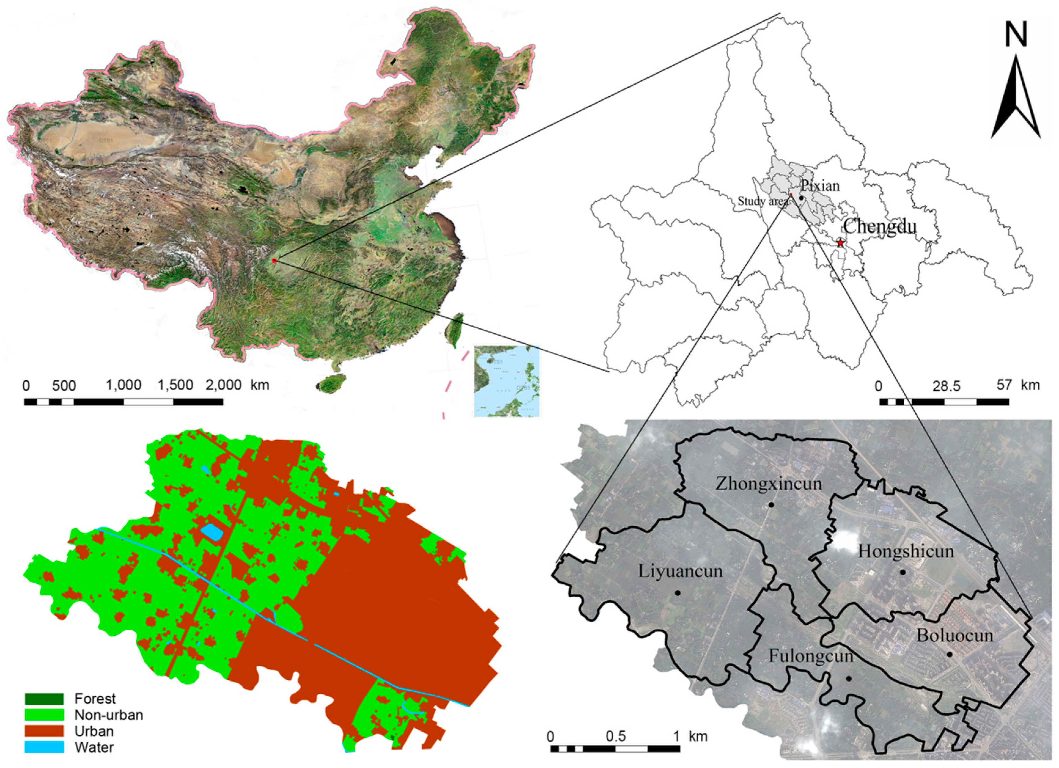
2.1. Study Area

The study was carried out on the rural–urban fringe of Chengdu, which is located in Sichuan province, southwestern China (Figure 1). The area of the city is 12,121 km², with a population of 14,657,500 inhabitants [22]. The study area is located in Pitong Town, a rural–urban fringe area in the city, and includes five villages named Zhongxing, Liyuan, Hongshi, Boluo, and Fulong. These five villages together have an area of approximately 6.35 km² and a population of 17,969 inhabitants. Chengdu Plain is the largest plain in southwest China, characterized by a dense river network, fertile soil, and a long farming history, which makes it one of the major agricultural areas of commodity grain and oil production in the country. The city is facing rapid urban expansion driven by the development strategy for western China. The urbanization rate increased from 33.3% in 2005 to 47.7% in 2015, and the rural population decreased by 13.4 million during this period [23]. In the context of rapid urbanization, farmlands, wastelands, and forest areas have been reducing at an alarming rate to meet the growing need for urban land. Therefore, Pitong Town exemplifies fast urbanization and the conflicts in rural–urban fringe zones. Moreover, it also represents the common issues faced by developing countries experiencing urban expansion. Considering all these conditions, we selected this area as the case study to examine the impacts of spatial extent when simulating urban growth.

2.2. Data and Methodology

2.2.1. Data

The land use data were obtained from the classification of the Thematic Mapper satellite images for December 2005, November 2010, December 2012, and December 2015. Based on the quality of the images and the IDRISI 17.0 precision test, the raster grid cell was set as 10 m × 10 m. A grid in the images was equal to a cell in the CA model, with the land use type as the state of the cell. The land use types include farmland, wasteland, natural water, forest, and built-up areas. Farmlands and wastelands were aggregated as a “non-urban” land use type, while natural waters and forests were classified as a restricted area, as no development is allowed according to regulations. The transition matrices of the land use types were calculated for three periods, i.e., 2005–2010, 2005–2012, and 2010–2012.

2.2.2. Model Framework

The Markov–CA model was used as the modeling method in this study. The land use data for 2005, 2010, and 2012 were used to calibrate the models of different spatial extents, while the data for 2015 were used to compare the simulation accuracy of the calibrated models. Two models were developed, at the city scale for Chengdu as a whole and at the village scale for the study area only. The simulation results for the two simulated spatial extents were then compared and discussed.

The driving factors of the land use changes considered in this study include: (1) variables representing the proximity to various types of centers, i.e., the distance to the city center $(d_{\mathrm{city}})$, the town center $(d_{\mathrm{town}})$, and the rail station $(d_{\mathrm{stations}})$; (2) variables representing the proximity to the transportation networks, including the distance to main roads $(d_{\mathrm{road}})$, railways $(d_{\mathrm{railways}})$, and highways $(d_{\mathrm{highways}})$; and (3) the distances to rivers $(d_{\mathrm{rivers}})$ and constructed land $(d_{\mathrm{constructions}})$. The slope is not considered because the advances in construction and farming techniques have reduced the impact of land slope on the efficiency of land use. The Markov transition matrices were evaluated at both the spatial extents of the city and the village. The simulation results for the urban growth until 2015 were compared between the two models.

2.2.3. Model Calibration

The amount of land use conversion in each period was calculated using the Markov transition matrix, which compares the previous and present land use patterns [24]. The transition matrix shows the conversion between each land use type in different time periods [25]. The amount of change was then distributed to individual land cells in the next step.

The allocation of land use changes was based on the calculation of the conversion potential scores of the cells, which were assessed by multi-criteria evaluation (MCE) [26]. In the MCE, the effects of all influencing factors are combined using the weighted linear method. The conversion potential score was calculated for each land cell (10 m × 10 m). The potential for cell i to be allocated with a particular land use type (${\mathrm{S}}_{\mathrm{o}}$) can be calculated as follows [27]:

$${\mathrm{S}}_{\mathrm{oi}}={{\displaystyle \sum }}_{\mathrm{t}=1}^{\mathrm{n}}{\mathrm{F}}_{\mathrm{ti}}{\mathrm{W}}_{\mathrm{t}}$$

(1)

where n is the number of cells in the defined neighborhood; ${\mathrm{F}}_{\mathrm{ti}}$ is the potential of factor t being normalized to 0 to 255 by the fuzzy clustering module; and ${\mathrm{W}}_{\mathrm{t}}$ denotes the weight of factor t. The weights were decided by the conversion from the cells in the existing data (

Table 1. The weight of the driving factor.

${\mathit{d}}_{\mathbf{city}}$	${\mathit{d}}_{\mathbf{town}}$	${\mathit{d}}_{\mathbf{stations}}$	${\mathit{d}}_{\mathbf{road}}$	${\mathit{d}}_{\mathbf{railways}}$	${\mathit{d}}_{\mathbf{highways}}$	${\mathit{d}}_{\mathbf{rivers}}$	${\mathit{d}}_{\mathbf{constructions}}$
0.229	0.168	0.194	0.285	−0.117	−0.094	0.186	0.151

) [28].

The simulation then increases or decreases the amount of each land use according to the potential score. In other words, if the cell has a score of 255 (the highest probability of becoming an integral unit) and a lower score for a non-established cell, then the cell will be converted to the established cell at the next stage. High-potential cells are sequentially converted until the total amount of land conversion decided in the previous step is reached. Besides the factor weight, the selection of a proper neighborhood configuration is also necessary for an accurate simulation. Five neighborhood configurations were tested in this study: 3 × 3, 4 × 4, 5 × 5, 6 × 6, 7 × 7, 8 × 8, 9 × 9, and 10 × 10.

The Kappa consistency coefficient was applied to quantify the similarity between the actual land use changes and the simulation results. In this study, the Cramer’s V correlation coefficient was used to measure the Kappa consistency. By overlapping the land use graphs and Cramer’s V correlation analysis, this method quantifies the degree of matching between the actual land use changes and the simulated results from two spatial extents [27]:

$$\mathrm{V}=\sqrt{\frac{{\mathrm{x}}^2}{\mathrm{N}\left(\min \left(\mathrm{m},\mathrm{n}\right)-1\right)}}$$

(2)

in which ${\mathrm{x}}^2$ is derived from chi-square analysis; N is the total number of cells in the map; m and n are the numbers of categories i and j, respectively.

3. Results

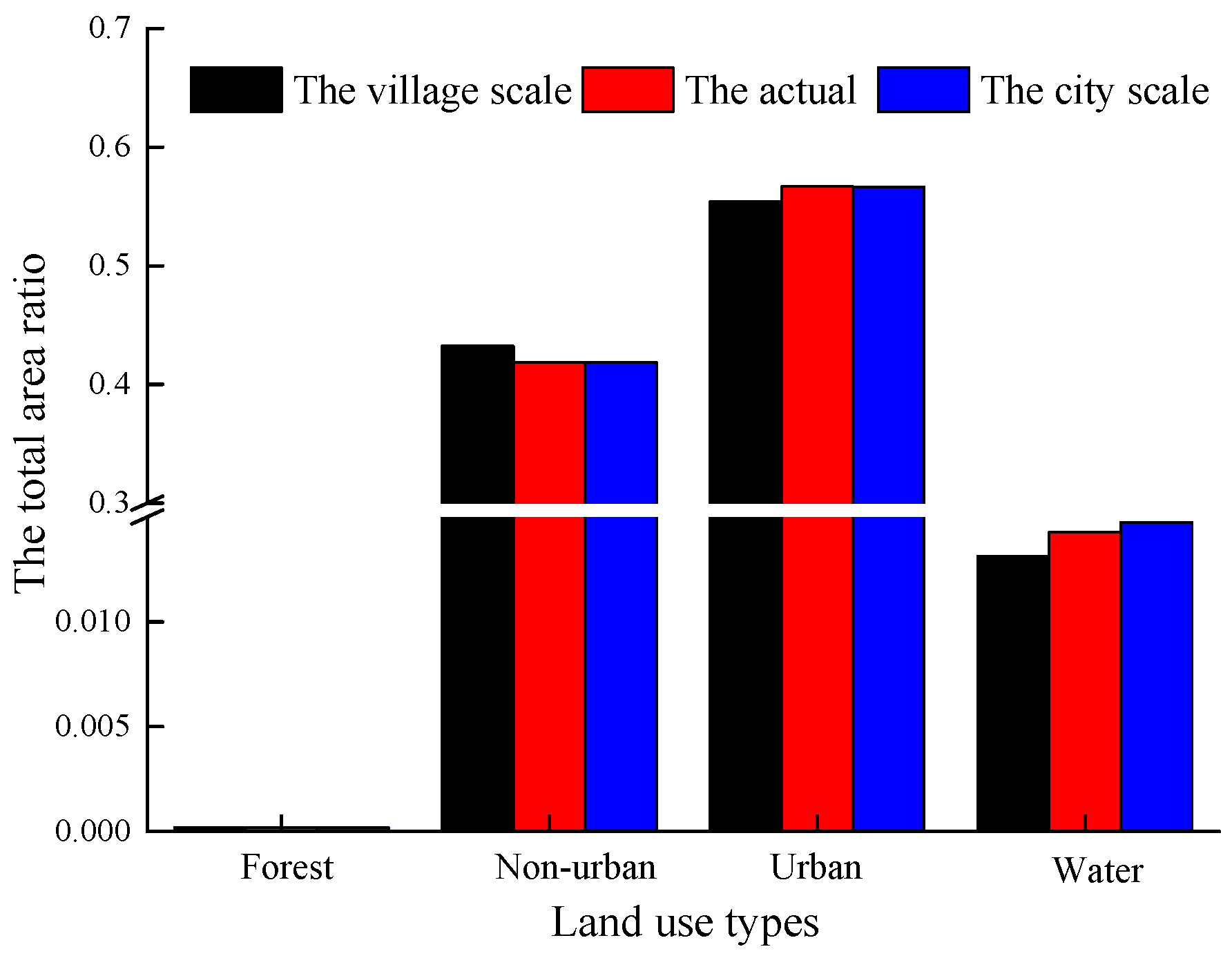
3.1. Amount of Land Use Change according to the Markov Model

Table 2. Markov transition matrices for the period of 2012–2015.

Land Use	Transition Matrix at the City Level				Transition Matrix at the Village Level
	Forest	Non-Urban	Urban	Water	Forest	Non-Urban	Urban	Water
Forest	0.747	0.209	0.037	0.007	1.000	0.000	0.000	0.000
Non-urban	0.148	0.461	0.351	0.040	0.000	0.901	0.099	0.000
Urban	0.036	0.364	0.580	0.020	0.000	0.005	0.995	0.000
Water	0.024	0.193	0.109	0.674	0.000	0.000	0.030	0.971

shows the Markov transition matrices derived from the spatial extents of the city and the villages for the period between 2012 and 2015, which was assumed to be the same as the transitions from 2005 to 2012.

Table 2 shows that the urban land increased prominently in the study period and the non-urban land was the main source of land conversion in both the city and the villages. Besides, the area of water bodies reduced in both the city and the villages. There were also several differences in land use changes at the two spatial extents. The non-urban land increased at the city level but decreased at the village level. The urban land was the main direction of change for non-urban land, accounting for 29.62% at the city level and 0.55% at the village scale. These changes can be attributed to the land consolidation of hollow villages, which aimed to promote the re-use of abandoned land in Chengdu. Another related trend was the reclamation of industrial and mining wastelands, promoted by Sichuan province since 2014. Since the land reclamation was balanced at the city level, 14.77% of the forest land was converted to non-urban areas, while no such change at the village scale was observed.

The actual extent of land use changes was obtained by multiplying the probabilities in the transition matrix with the number of cells of the corresponding land use type in 2012. The development probability of a cell in a certain direction was estimated using the Markov module (Figure 2). The probability of non-urban land being converted into urban land seemed higher when estimated at the village level than at the city level. The cells with relatively higher conversion probability were concentrated at the rural–urban fringe, where the development is rapid.

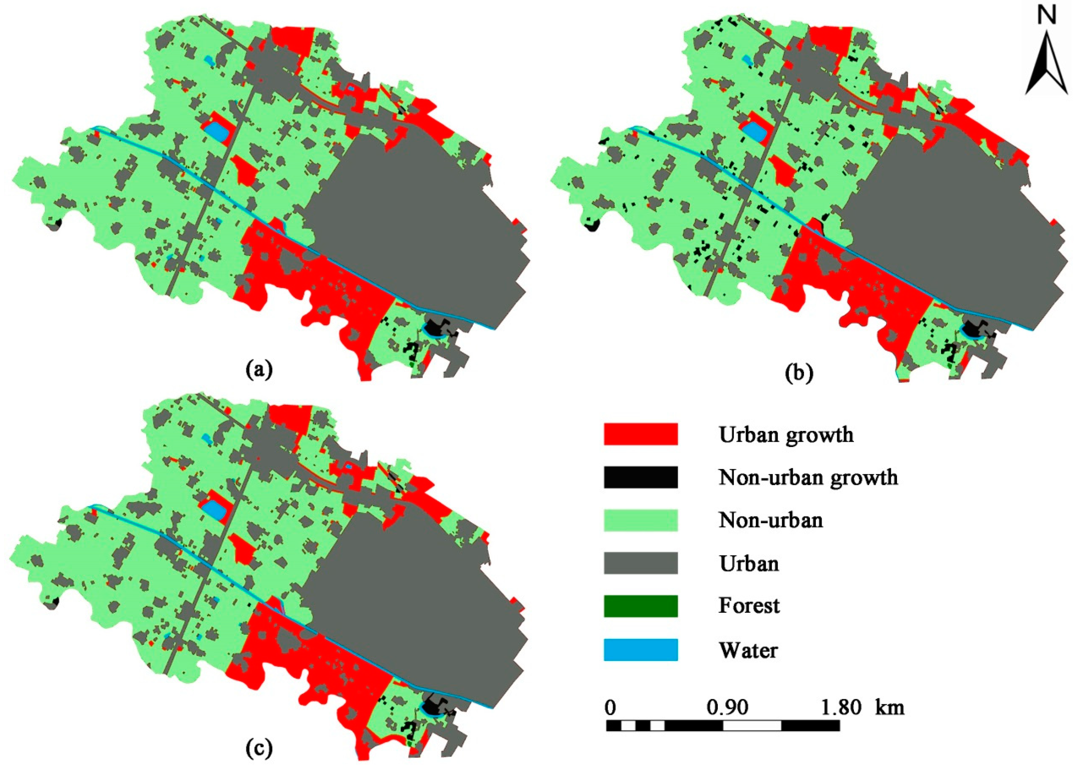
3.2. Simulated Spatial Distribution according to the CA Model

The driving factors were measured using a raster database. The values were standardized to 0–255 by the fuzzy module (Figure 3). These maps were then combined to generate weighted conversion potential estimates, which were utilized in the two CA models to allocate the land use conversion. At this stage, the different neighborhood configurations were compared. The models were run with one of the five neighborhood configurations each time, and the Kappa values of the simulation results were compared (

Table 3. The neighborhood configurations with Kappa indices.

The Kappa Value	The Neighborhood Configurations
	3 × 3	4 × 4	5 × 5	6 × 6	7 × 7	8 × 8	9 × 9	10 × 10
Village model	0.835	0.896	0.925	0.954	0.921	0.870	0.854	0.783
City model	0.603	0.685	0.700	0.741	0.753	0.733	0.710	0.752

). The neighborhood configuration of 6 × was selected, considering both the performance of the village and the city model.

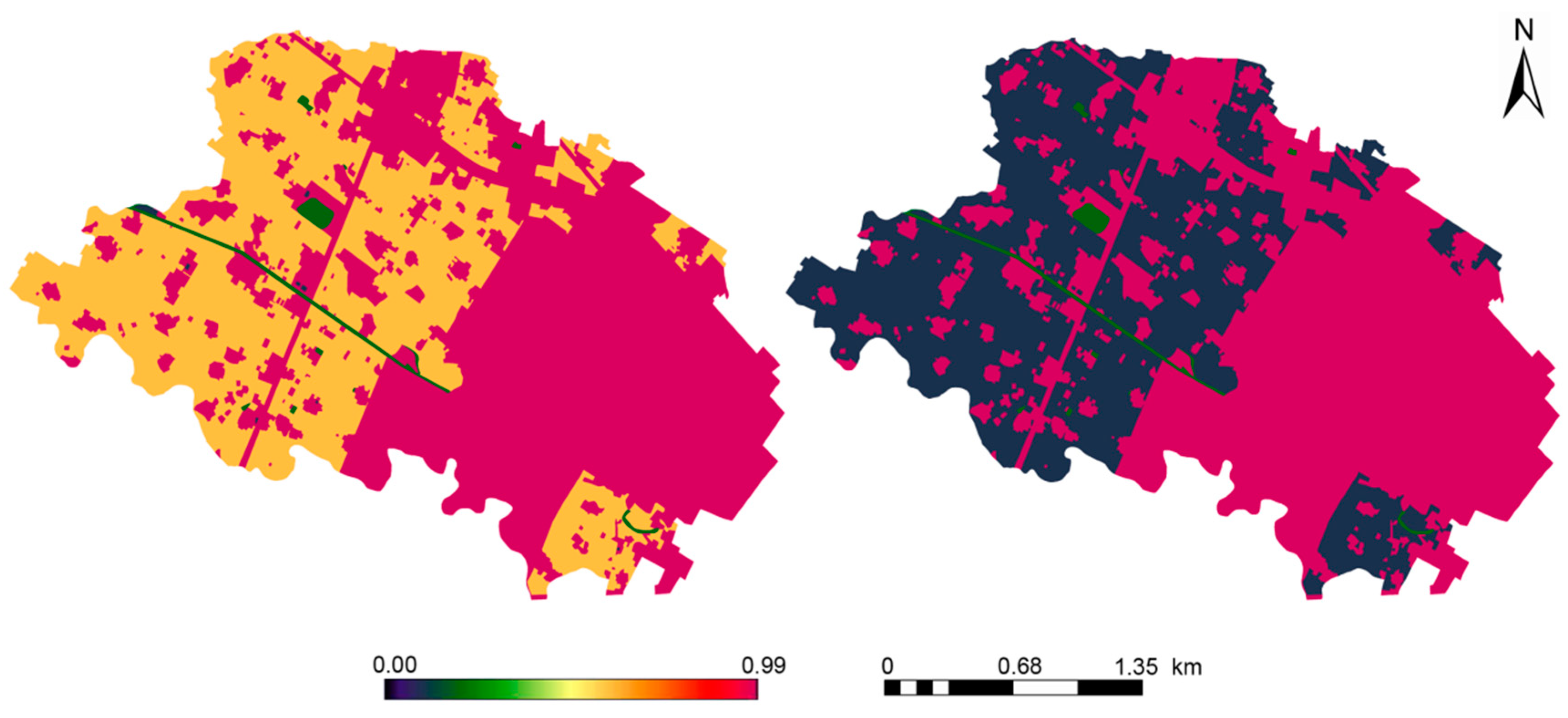
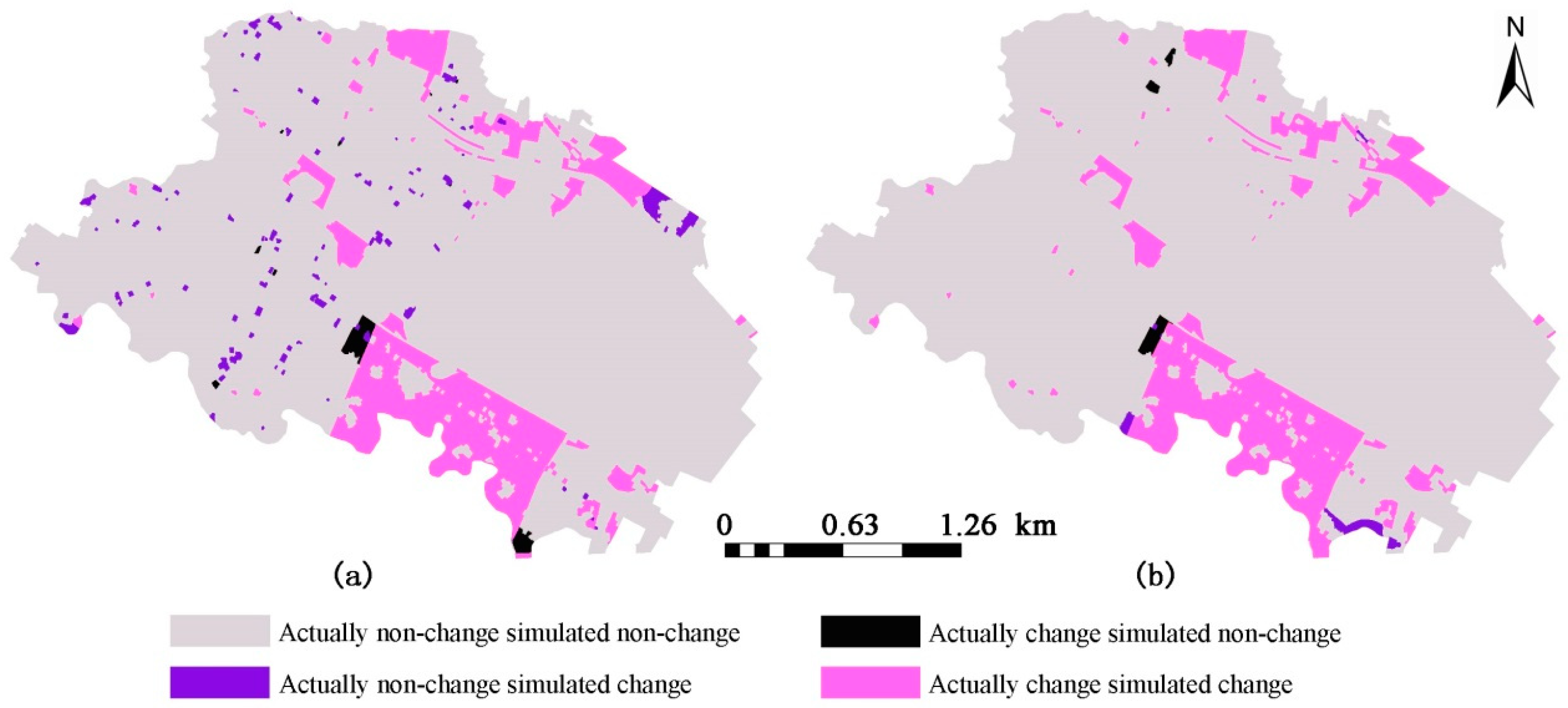
3.3. Comparing the Model Performance at the Two Spatial Extents

The calibrated Markov–CA models were then applied to simulate the land use changes until 2015 and compared (Figure 3). Significant differences were observed in the results of the two models. Both models predicted a continuous decrease in the non-urban land and forest area and an increase in urban land. The actual area of development in the study area was 0.72 km² between 2005 and 2015 based on the land use data for the two years (Figure 3a). The predicted area of development was 0.80 and 0.86 km² in the city model and the village model, respectively. Therefore, in terms of the total amount of urban expansion, the city model produced a better result.

The accuracy in the spatial distribution of the land use changes was verified by overlapping the actual changes with the simulated changes between 2005 and 2015 (Figure 4). The hotspot of urban growth in this rural–urban fringe area was in the south, close to the city center of Chengdu. It turns out that the accuracy of the results produced by the city model was 7.33% higher than that of the village model (Figure 5). Therefore, the simulation at the city extent produced more accurate predictions in terms of both the total area of urbanization and the location of changes.

4. Discussion

There are several reasons that may explain the differences between the simulation results at the different spatial extents. The first reason is related to the tight connection between life and the economy at the rural–urban fringe and the city center. Surveys have found that people living at the rural–urban fringe mainly rely on the city to make a living, as well as for the provision of supporting facilities [29]. Correspondingly, the function of the town centers is gradually weakened [30]. Therefore, taking the whole city area into consideration helps produce better predictions. Secondly, the changing trends in land demand at the rural–urban fringe may also affect the performance of the simulations. Most residents of the rural–urban fringe in Sichuan province are migrant workers, many of whom leave behind abandoned residential areas. This leads to a phenomenon commonly known as the ‘hollowing village’ [31,32,33]. The provincial government began to promote land reclamation in hollowing villages from 2008, and the Pi district was designated as a showcase area [34]. As a result, many small settlements were restored to arable land.

However, with the rapid economic development in Sichuan province, the number of migrant workers gradually increased after 2012 [35]. The demand for rural construction land gradually increased in the rural–urban fringe zone of Chengdu, and the decline of small settlements was not obvious after this time [36]. Due to the large base area of Chengdu, the urban land was not significantly restored to arable land. Therefore, the accuracy of the simulation using the smaller spatial scale was reduced.

The findings of this research are also limited in several ways. Firstly, as mentioned in the introduction, numerous approaches to developing transition rules have been put forward throughout the development of the CA models. This study adopted the Markov-CA approach, and was therefore subject to further examination regarding whether the findings could also apply to CA models with other transition rules such as MCE-CA and PCA-CA. Besides, only two spatial extents were tested and compared in our work. Building on our results, it would also be interesting to examine the simulation results at more spatial extents such as the county level, the province level, etc.

5. Conclusions

This study demonstrated that the simulation accuracy of land use changes was higher when conducted at a larger spatial extent, in this case, at the city level compared with the village level. Both the total amount of land use change and the spatial distribution of the changes better matched reality. The simulation at the larger extent took greater consideration of the consistency of the overall development.

Land use change in rural–urban fringe areas is a key aspect in the development of a city. This finding is useful for urban planners and policymakers developing urban models that evaluate the directions of development and make land management decisions. Nonetheless, the study was limited, since only the case of Chengdu was used, which may not represent the situation in other cities and regions around the world. Studies of more cities and regions with different socio-economic characteristics are needed in the future.

References

1. Crossman, N.D.; Bryan, B.A.; Ostendorf, B.; Collins, S. Systematic landscape restoration in the rural-urban fringe: Meeting conservation planning and policy goals. Biodivers. Conserv. 2007, 16, 3781–3802. [Google Scholar] [CrossRef]
2. Yang, Y.; Wang, Y.; Wu, K.; Yu, X. Classification of Complex Rural-urban fringe Land Cover Using Evidential Reasoning Based on Fuzzy Rough Set: A Case Study of Wuhan City. Remote Sens. 2016, 8, 304. [Google Scholar] [CrossRef]
3. Kong, C.; Lan, H.; Yang, G.; Xu, K. Geo-environmental suitability assessment for agricultural land in the rural-urban fringe using BPNN and GIS: A case study of Hangzhou. Environ. Earth Sci. 2016, 75. [Google Scholar] [CrossRef]
4. Liu, Z.; Robinson, G.M. Residential development in the peri-rural-urban fringe: The example of Adelaide, South Australia. Land Use Policy 2016, 57, 179–192. [Google Scholar] [CrossRef]
5. Dietzel, C.; Clarke, K. The effect of disaggregating land use categories in cellular automata during model calibration and forecasting. Comput. Environ. Urban Syst. 2006, 30, 78–101. [Google Scholar] [CrossRef]
6. He, C.; Okada, N.; Zhang, Q.; Shi, P.; Li, J. Modelling dynamic urban expansion processes incorporating a potential model with cellular automata. Landsc. Urban Plan. 2008, 86, 79–91. [Google Scholar] [CrossRef]
7. Syphard, A.D.; Clarke, K.C.; Franklin, J. Using a cellular automaton model to forecast the effects of urban growth on habitat pattern in southern California. Ecol. Complex. 2005, 2, 185–203. [Google Scholar] [CrossRef]
8. Li, X.; Yeh, A.G.O. Data mining of cellular automata’s transition rules. Int. J. Geogr. Inf. Sci. 2004, 18, 723–744. [Google Scholar] [CrossRef]
9. Gallent, N.; Shaw, D. Spatial planning, area action plans and the rural-urban fringe. J. Environ. Plan. Manag. 2008, 50, 617–638. [Google Scholar] [CrossRef]
10. Jafari, M.; Majedi, H.; Monavari, S.; Alesheikh, A.; Zarkesh, K.M. Dynamic Simulation of Urban Expansion Based on Cellular Automata and Logistic Regression Model: Case Study of the Hyrcanian Region of Iran. Sustainability 2016, 8, 810. [Google Scholar] [CrossRef]
11. Tian, G.; Ma, B.; Xu, X.; Liu, X.; Xu, L.; Liu, X.; Xiao, L.; Kong, L. Simulation of urban expansion and encroachment using cellular automata and multi-agent system model-A case study of Tianjin metropolitan region, China. Ecol. Indicators 2016, 70, 439–450. [Google Scholar] [CrossRef]
12. Yang, X.; Chen, R.; Zheng, X.Q. Simulating land use change by integrating ANN-CA model and landscape pattern indices. Geom. Natl. Hazards Risk 2016, 7, 915–918. [Google Scholar] [CrossRef]
13. White, R.W.; Engelen, G. Cellular automaton as the basis of integrated dynamic regional modeling. Environ. Plan. B Plan. Des. 1997, 24, 235–246. [Google Scholar] [CrossRef]
14. Wu, F.; Webster, C.J. Simulation of land development through the integration of cellular automata and multi-criteria evaluation. Environ. Plan. B Plan. Des. 1998, 25, 103–126. [Google Scholar] [CrossRef]
15. Clark, K.C.; Gaydos, L.J. Loose-coupling a cellular automation model and GIS: Long-term urban growth prediction for San Francisco and Washington/Baltimore. Int. J. Geogr. Inf. Sci. 1998, 12, 699–714. [Google Scholar] [CrossRef] [PubMed]
16. Yeh, A.G.O.; Li, X. A cellular automata model to simulate development density for urban planning. Environ. Plan. B Plan. Des. 2002, 29, 431–450. [Google Scholar] [CrossRef]
17. Zhao, Y.; Murayama, Y. A constrained CA model to simulate urban growth of the Tokyo Metropolitan Area. In Proceedings of the 9th International Conference on Geocomputation, National University of Ireland, Maynooth, Ireland, 3–5 September 2007. [Google Scholar]
18. Campagnaro, T.; Frate, L.; Carranza, M.L.; Sitzia, T. Multi-scale analysis of alpine landscapes with different intensities of abandonment reveals similar spatial pattern changes: Implications for habitat conservation. Ecol. Indicators 2017, 74, 147–159. [Google Scholar] [CrossRef]
19. Brown, D.G.; Page, S.; Riolo, R.; Zellner, M.; Rand, W. Path dependence and the validation of agent-based spatial models of land use. Int. J. Geogr. Inf. Sci. 2005, 19, 153–174. [Google Scholar] [CrossRef]
20. Sang, L.; Zhang, C.; Yang, J.; Zhu, D.; Yun, W. Simulation of land use spatial pattern of towns and villages based on CA-Markov model. Math. Comput. Model. 2011, 54, 938–943. [Google Scholar] [CrossRef]
21. Huang, Y.; Nian, P.; Zhang, W. The prediction of interregional land use differences in Beijing: A Markov model. Environ. Earth Sci. 2015, 73, 4077–4090. [Google Scholar] [CrossRef]
22. Chengdu Bureau of Statistics; Chengdu Statistical Society. Chengdu Statistical Yearbook; China Statistics Press: Beijing, China, 2016.
23. Gao, X.; Xu, A.; Liu, L.; Deng, O.; Zeng, M.; Ling, J.; Wei, Y. Understanding rural housing abandonment in China’s rapid urbanization. Habitat Int. 2017, 67, 13–21. [Google Scholar] [CrossRef]
24. Kamusoko, C.; Aniya, M.; Adi, B.; Manjoro, M. Rural sustainability under threat in Zimbabwe-Simulation of future land use/cover changes in the Bindura district based on the Markov-cellular automata model. Appl. Geogr. 2009, 29, 435–447. [Google Scholar] [CrossRef]
25. Guan, D.; Li, H.; Inohae, T.; Su, W.; Nagaie, T.; Hokao, K. Modeling urban land use change by the integration of cellular automaton and Markov model. Ecol. Model. 2011, 222, 3761–3772. [Google Scholar] [CrossRef]
26. Yagoub, M.M.; Al Bizreh, A.A. Prediction of Land Cover Change Using Markov and Cellular Automata Models: Case of Al-Ain, UAE, 1992–2030. J. Indian Soc. Remote Sens. 2014, 42, 665–671. [Google Scholar] [CrossRef]
27. Ku, C. Incorporating spatial regression model into cellular automata for simulating land use change. Appl. Geogr. 2016, 69, 1–9. [Google Scholar] [CrossRef]
28. Li, X.; Lin, J.; Chen, Y.; Liu, X.; Ai, B. Calibrating cellular automata based on landscape metrics by using genetic algorithms. Int. J. Geogr. Inf. Sci. 2013, 27, 594–613. [Google Scholar] [CrossRef]
29. Gant, R.L.; Robinson, G.M.; Fazal, S. Land-use change in the ‘edgelands’: Policies and pressures in London’s rural-urban fringe. Land Use Policy 2011, 28, 266–279. [Google Scholar] [CrossRef]
30. Porta, J.; Parapar, J.; Doallo, R.; Barbosa, V.; Santé, I.; Crecente, R.; Díaz, C. A population-based iterated greedy algorithm for the delimitation and zoning of rural settlements. Comput. Environ. Urban Syst. 2013, 39, 12–26. [Google Scholar] [CrossRef]
31. Liu, Y.; Liu, Y.; Chen, Y.; Long, H. The process and driving forces of rural hollowing in China under rapid urbanization. J. Geogr. Sci. 2010, 20, 876–888. [Google Scholar] [CrossRef]
32. Long, H.; Li, Y.; Liu, Y.; Woods, M.; Zou, J. Accelerated restructuring in rural China fueled by ‘increasing vs. decreasing balance’ land-use policy for dealing with hollowed villages. Land Use Policy 2012, 29, 11–22. [Google Scholar] [CrossRef] [Green Version]
33. Sun, H.; Liu, Y.; Xu, K. Hollow villages and rural restructuring in major rural regions of China: A case study of Yucheng City, Shandong Province. Chin. Geogr. Sci. 2011, 21, 354–363. [Google Scholar] [CrossRef] [Green Version]
34. Liu, Y.; Zhang, F.; Zhang, Y. Appraisal of typical rural development models during rapid urbanization in the eastern coastal region of China. J. Geogr. Sci. 2009, 19, 557–567. [Google Scholar] [CrossRef]
35. Xing, C.; Zhang, J. The preference for larger cities in China: Evidence from rural-urban migrants. China Econ. Rev. 2017, 43, 72–90. [Google Scholar] [CrossRef] [Green Version]
36. Chen, R.; Ye, C.; Cai, Y.; Xing, X.; Chen, Q. The impact of rural out-migration on land use transition in China: Past, present and trend. Land Use Policy 2014, 40, 101–110. [Google Scholar] [CrossRef]
Figure 1. Location of Chengdu and the study area.
Sustainability 10 04758 g001
Figure 2. Markov conditional probability of the urban type: left villages and right Chengdu.
Sustainability 10 04758 g002
Figure 3. Comparison between the actual (a) and the simulated growth (b,c) from 2005 to 2015, (b) Simulation results of the village model, (c) Simulation results of the city model.
Sustainability 10 04758 g003
Figure 4. Comparison of the actual land use changes 2005–2015 and the simulated changes in (a) the city model and (b) the village model.
Sustainability 10 04758 g004
Figure 5. Comparison of the ratios of the four types of land in reality and simulation.
Sustainability 10 04758 g005