Article

The Active Power Losses in the Road Lighting Installation with Dimmable LED Luminaires

Institute of Electrical Power Engineering, Lodz University of Technology, 90-924 Łódź, Poland
*
Author to whom correspondence should be addressed.
Sustainability 2018, 10(12), 4742; https://doi.org/10.3390/su10124742
Submission received: 9 November 2018 / Revised: 3 December 2018 / Accepted: 9 December 2018 / Published: 12 December 2018
(This article belongs to the Collection Power System and Sustainability)

Abstract

:
In accordance with the requirements of PN EN 13201-5 standard for road lighting installation, energy performance indicators should be descripted. In order to calculate energy performance indicators, it is necessary to know the active power of the road lighting system. The above standard does not specify whether active power losses should be taken into account in calculations. The main purpose of the article is to estimate the active power losses in the road lighting installation. The article presents methods for calculating active power losses, taking into account losses in all main elements of the installation. The obtained calculation results show the relationship between active power losses and the power of luminaires, their number and spacing between poles. Calculations of active power losses were made for single-phase and three-phase installations. The active power losses in a three-phase system do not exceed 1.5% and in a single-phase installation they may be greater than 7%. Therefore, in order to obtain exact values of energy performance indicators (and also predict electricity consumption), active power losses should be taken into account in calculations. In addition, a comparative analysis of the effect of luminaires dimming and active power losses on annual CO2 emissions was made. Not taking into account the active power losses in the calculation of the lighting installation’s power, for single-phase installations in particular, understates the calculated value of CO2 emissions by more than 6%.

1. Introduction

In each electrical installation, the losses of active power occur due to the current flowing through the components of the system with a certain resistance and reactance. The power losses are caused by the flow of active and reactive power in the wires and cables, in the protection devices, in the executing components (contacts), etc. [1,2,3,4]. They cause, among others, a reduction in network bandwidth and warming up of wiring. Consequently, the active power losses will worsen the actual energy efficiency of the installation, because they are not included in the calculations. The practice of determining electrical power losses concerns the sum of the losses in the individual network elements [5,6]. In order to obtain a more accurate determination of power losses, the physical phenomena occurring within a given network elements are taken into account. For some receivers, electricity power losses may significantly affect their efficiency, e.g., luminaires working in road lighting.
The losses of active power in a road lighting system depend on the complexity of the network, the number of circuits and the number of luminaires in the individual circuits, the power supply dimming used, the reactive power level in the network, etc. Reduction of active power losses in lighting networks can be achieved through the use of regulated devices [7,8] and by reducing the reactive power in these networks [9,10,11,12]. In this way, one takes into account the skin effect occurring in the conductor of the cable (wire) and its results [5]. The energy efficiency improvement of a lighting installation is the focus of many programs funded by the European Commission. Thanks to this, it will be possible to improve the efficiency of an electricity receiver, to reduce the costs of working [13,14,15,16,17,18]. Energy efficiency improvement is possible by using lighting dimming systems [7,8,17]. The degree of energy efficiency is characterized by the EEI coefficient (Energy Efficiency Index) [15]. An important aspect of the decision-making process is to provide investors with a potential tool for evaluating it. In the investment decision-making process, the labelling of the products plays an important role in facilitating the identification of the most effective solutions [16]. Another aspect of improving the energy efficiency of a lighting installation is that it is designed to maximize the efficiency of the light flux emitted in the surrounding space while minimizing its losses [16].
Road lighting installations are now being attributed the role of one of the road safety elements, which ensures the safe movement of all users in outdoor spaces in the evening. At the same time, energy consumption is required to be as low as possible. The dynamic development of lighting technologies has created a big potential of the so-called “intelligent lighting systems,” especially in LED technology. The widespread use of such solutions depends, to a large extent, on their price. One example of intelligent lighting systems is the use of luminaires equipped with individual systems of power reduction to a set schedule light. Lighting schedules may be the same for each day and season, or may be different for each period. Lighting schedule is referred to the degree of reduction of power and luminous flux of luminaries in specified periods of the evening. The degree of power reduction should not worsen the lighting conditions specified in [15]. Each way of reducing the power of the luminaire brings measurable benefits in terms of reducing the electricity consumption of the lighting system and, thus, improves the energy efficiency of the installation. Often, in the practice of road lighting modernization, care is not taken to ensure compliance with the requirements of [19], with reduced power and light levels. This standard allows the road/street lighting class to be reduced in order to improve the energy efficiency of the installation. The energy efficiency should also take into account the loss of active power when it becomes important. The standard [19] in Sheet 5 identified indicators for assessing the energy efficiency of road lighting, taking into account the energy consumption while maintaining the appropriate lighting parameters on the road.
So far, there has been no detailed investigation in the literature about the effect of LED lighting dimming level on the active power losses in lighting installations. The increase in power losses will result in an increase in active power and charges for consumed electricity. Until now, when calculating the power losses in lighting networks, it was assumed that the network would receive constant power from the rated light sources or luminaires throughout the lighting period. During lighting operation, the rated power of the lighting equipment may change during their lifetime. In addition, at night time, the supply voltage may be higher than the rated network voltage, which means greater active power consumption, higher power currents and higher power losses. For LED dimming led luminaires, power losses are dependent on the lighting time and the light power at each reduction stage.
This article has the following structure. Section 2 includes information on how to calculate the power density indicator in accordance with the [19] standard for the road lighting installations and contains the methodology for calculating power losses in individual elements of the lighting installation. Section 3 presents the characteristics of the tested luminaire and the results of calculations of power losses for three-phase and single-phase installations. Moreover, the results of calculations of the power losses dependence on the distance between the poles are presented. It also contains the results of calculations of CO2 emissions for lighting installations without dimming and for the assumed lighting schedule. Section 4 presents a proposal to estimate the level of active power losses for a given lighting circuit configuration.

2. Calculation Method of Power Density Indicator and Active Power Losses in Road Lighting Installation

2.1. Calculation Method of Power Density Indicator by PN-EN 13201-5

One of the coefficients for assessing the energy efficiency of a lighting installation, proposed by Sheet 5 of [19], is the power density indicator Dp. The Dp indicator determines the electrical power that is needed to provide an adequate level of road illumination. It is calculated as the quotient of the active power P of the lighting installation and the sum of the products of the average illumination on the i-th and the horizontal planes of Ei and the area of those planes Ai according to the relation [19]:
D p = P i = 1 n ( E i ¯ A i ) .
The active power of the lighting system is calculated as the sum of the power of the lighting points Pk and the power of other devices necessary to operate the lighting system Pad.
P = k = 1 n l u P k + P a d .
It seems that the active power losses in the power supply can be taken as a component of the Pad, as the power supply of the luminaires together with the safety devices and connectors is essential for the operation of the lighting system. It has therefore been found that the losses of active power in the light source installation may be relevant in determining the total active power P of the illumination using in Equations (1) and (2).
This article presents a detailed analysis of the active power losses occurring in lighting installations with LED luminaires and individual power reduction systems. Two cases of power supply circuits were considered in actual installations: Three-phase and single-phase power supply. Most manufacturers of road lighting luminaires provide luminaire rated parameters for 100% dimming. Often, there is no information on the dimming characteristics of the luminous intensity dependence of the luminaire’s power for different levels of reduction. Data concerning the change of important electrical parameters of the installation as a dimming function, such as the power factor (PFD and PFDD) and the total harmonic distortion factor THDI [20], active power losses, etc., are also not known. These characteristics are important in assessing energy efficiency and to ensure proper performance of the lighting system, which guarantees the assumed durability and functionality. In the article, the extent to which active power losses in the installation with road lighting luminaires with dimmable LED luminaires may affect the active power consumed for lighting.

2.2. Calculation Method of Active Power Losses in Road Lighting Installation

The lighting circuit consists of the following components: The power cable protection in the lighting panelboard, relay dimming by astronomical clock (or other dimming device), three-phase feeder wiring, the pole protection (placed in the pole post), the wire connecting the pole plate with luminaire, and the luminaire. Figure 1 shows, schematically, an example of a road lighting installation with the main components. Total power losses are included in the calculation of total power losses occurring in all the aforementioned components of the lighting circuit. The power losses in the neutral conductor of the cable (wire) for the three-phase power supply network was also taken into account. Losses in the neutral conductor are caused by the flow of higher zero sequence harmonic and their order is a multiple of three. The LED luminaire with a power supply device is a nonlinear element that generates disturbances to the supplying network (higher harmonics). Depending on the constructive solution, the THDI determining the value of these disorders is in the range from several to several dozen percent, which is confirmed by test results presented in [21].
The total power loss of the lighting installation ΔPTOTAL can be determined from the following relationship:
Δ P T O T A L = Δ P C A B L E + Δ P N E U T R A L + Δ P W I R E + Δ P P P B + Δ P P P O L E + Δ P R E L A Y .
For three-phase lighting, installation power losses in the feeder wiring can be determined from the relationship [4]:
Δ P C A B L E = 3 l γ C S C [ n 2 ( l 01 + l l ) + n ( n 1 ) ( 2 n 1 ) 2 ] I L u m 2 .
In the case of single-phase installation, the power losses can be determined by the following formula [4].
Δ P C A B L E = 2 l γ C S C [ n 2 ( l 01 l ) + n ( n 1 ) ( 2 n 1 ) 6 ] I L u m 2 .
Power losses in the neutral conductor of feeder wiring can be determined from the dependence [4]:
Δ P N E U T R A L = l γ C S C [ 9 n 2 + l 01 l + n ( 3 n 1 ) ( 6 n 1 ) 2 ] h = 3 I h L u m 2 ,
or
Δ P N E U T R A L = l γ C S C [ 9 n 2 + l 01 l + n ( 3 n 1 ) ( 6 n 1 ) 2 ] I N L u m 2 .
Power losses in the wire connecting the pole switchboard and luminaire are determined by the Equation (8).
Δ P W I R E = 2 I L u m 2 R P W = 2 l P W γ P W S P W I L u m 2 .
Power losses in protection in the lighting panelboard are determined by the following dependence:
Δ P P P B = 3 I L I 2 R P P B .
In case when the protection is realized by miniature circuit breaker (MCB):
R P P B = R M C B .
Knowing the rated active power losses of the minimal circuit breaker ΔPMCB given for its rated current IMCB can be determined by the following formula:
R M C B = Δ P M C B 3 I M C B 2 .
If the fuse is used to protect the feeder wiring of the lighting system:
R P P B = R P B F B + R P B F .
Resistance of fuse carrier can be determined from Equation (13) and resistance of fuse is calculated as (14).
R P B F B = Δ P P B F B I P B F B 2 .
R P B F = Δ P P B F I P B F 2 .
For protection in the pole the power losses are determined by below Equation (15).
Δ P P P B = 3 I L u m 2 R P P o l e .
In the case when the protection is realized by miniature circuit breaker (MCB):
R P P o l e = R M C B .
Knowing the rated active power losses of the miniature circuit breaker ΔPMCB given for its rated current IMCB can be determined by the following:
R M C B = Δ P M C B I M C B 2 .
If the fuse is used to protect the wire of the luminaire, the resistance of protection device is calculated as sum of fuse carrier and fuse resistance by Equation (18).
R P P B = R P B F B + R P B F
Resistance of fuse carrier is determined as:
R P B F B = Δ P P B F B I P B F B 2 .
Resistance of fuse is calculated by using of Equation (20).
R P B F = Δ P P B F I P B F 2 .
Power losses in relay are calculated by the below dependence.
Δ P R E L A Y = 3 I L I 2 R R .
Based on knowledge of the rated active power losses of the relay ΔPRR given for its rated current IR the relay resistance is calculated by the Equation (22).
R R = Δ P R R 3 I R 2 .
The number of light points is equivalent to the number of columns, since it is assumed that the luminaires are mounted on columns individually. For the above Equations (3) to (22), dependencies were used to calculate the active power losses in a three-phase system and single-phase road lighting.

3. Calculation Results of Active Power Losses in Road Lighting Installation

3.1. Characteristics of the Research Objects

In order to present the methods of calculation of power losses in the road lighting installation described in Section 3, calculations for three luminaires with adjustable luminous flux were made. Two dimming luminaires marked as LUM1 of rated power 32 W and LUM2 with a rated power of 85 W, an analogous dimming input in the scope of 1–10 V standard was used. The laboratory power supply was used as the source of the DC dimming voltage. The luminaire was powered using the Agilent 6834B power supply. Measurements of electrical and photometric parameters were made using the TOPAS 1000 electricity quality analyzer from LEM NORMA, the L-100 Luxmeter by SONOPAN and the Ulbricht sphere with a diameter of 2 m. The Agilent 6834B stabilized power supply enabled the luminaire to be supplied with uninterrupted sinusoidal voltage. The third luminaire marked LUM3 with a rated power of 140 W was equipped with a wireless power and luminous flux dimming system. The dimming was carried out using a program implemented on the server. The program enabled the dimming of the luminaire in the range from 10% to 100%, however, the power and luminous flux of the luminaire for particular dimming were not specified by the manufacturer. The measurements were taken for the entire dimming range, every 10%. The determination of dimming by means of percentages, as reported by the manufacturer, was adopted. This is also the most common way to describe dimming. The electrical and photometric parameters of the luminaires tested are presented in Table 1, Table 2 and Table 3 respectively.
The active power P of the luminaire marked LUM1 in the range of UC dimming voltages from 1 to 8 V is linear. In the range of UC from 8 to 10 V, the luminaire takes maximum power. The dependence of the current supplying of the luminaire from the dimming voltage is analogous to that for the active power (dependence is linear). Reactive power Q changes, within small limits, with the change of the dimming voltage UC. The next analyzed electric parameter was the total current harmonic distortion factor THDI. For UC dimming voltages with a value greater than 5 V, the THDI value of the current drawn from the network changes within small limits. In the range of the dimming voltage from 5 to 1 V, the value of THDI increases significantly from 13.907% for UC = 10 V to 38.007% for UC = 1 V. The reduction of the dimming causes a large change in the values of displacement power factor PFD and distorted power factor PFDD, as illustrated in Table 1. In the range of dimming voltages from 1 to 8 V, the value of the luminous flux increases linearly until the value reaches 2736 lm. Increasing the UC voltage above 8 V does not change the luminous flux. As one can see, UC = 1 V corresponds to 19% of rated power and 14% of luminous flux. This is the lower limit of dimming. The luminaire efficiency ηLum calculated as the quotient of luminous flux and active power ranges from 84.238 lm/W to 62.510 lm/W.
Table 2 presents the measured electrical and photometric parameters of the LUM2 luminaire with the rated active power equal to 85 W. For this luminaire, the parameters for the dimming voltage ranging from 2 to 10 V were measured. For the UC = 1 V voltage, the luminaire did not work stably, which was manifested by the unstabilized value of the luminous flux and the pulsation of the active power. Therefore, this point was omitted in the considerations. In the case of this luminaire, a linear dependence of active power, current and luminous flux on the dimming voltage was also found. The power supply used in this luminaire is equipped with a PFC (Power Factor Correction) system, which reduces the reactive power value along with the reduction of the dimming. This allows, practically, the constant value of displacement power factor PFD to be maintained. Decreasing the level of dimming causes the increase of the THDI value from the value of 13.319% to the value of 202.060%. This, in turn, reduces the value of distorted power factor value PFDD from 0.966 to 0.411. The luminous efficiency ηLum is in the range of 143.432 lm/W for UC = 10 V to 164.349 lm/W for UC = 2 V.
For luminaire marked LUM3, the active power of the luminaire varies linearly from 144.470 W (at 100% of dimming) to 27% of the starting power (at 10% of dimming). The reactive power of the luminaire varies much more slowly than the active power, reaching a minimum of about 79% of the initial value with a minimum of 10% dimming. Displacement power factor PFD of the luminaire decreases to 0.802, while the tgϕ to the level of 40% retains the value of ≤0.4, then rapidly grows almost three times beyond the initial value. The distorted power factor value PFDD varies in the range of 0.759–0.955. The value of this coefficient depends on the THDI current and decreases with its increase. The luminous flux of the luminaire is almost two times lower than the dimming of the luminaire, reaching about 70% of the initial flux at 50% of its value. For the considered luminaire, the luminous efficiency ηLum decreases with the increase of dimming from the value of 117.885 lm/W to the value of 97.467 lm/W. Finally, the luminous efficiency decreases by over 17%.

3.2. Active Power Losses Calculation Results of Three-Phase Lighting System

The calculations of active power losses were made for an exemplary three-phase road lighting system with different numbers of lighting points (luminaires) np consisting of 3 to 30 pieces. The number of light points was equivalent to the number of poles, since it is assumed that the luminaires are mounted on poles individually. The adopted length of feeder wiring between the luminaires was equal to 30 m. The distance of the first luminaire of the switchgear lighting adopted was also equal to 30 m. The installation was made of an aluminum cable with a cross section of 4 × 25 mm2 and a conductivity of 34 (m/Ω·mm2). It was assumed that the wire in the pole from the pole panelboard to the luminaire was a copper conductor with a cross-section of 1.5 mm2, 10 m in length and a conductivity of 56 (m/Ω·mm2). For the assumed parameters of the lighting system, the active power losses were determined in feeder wiring, wires in the poles, in protection of lighting switchboard, protection in the poles, relay, in neutral conductor of feeder wiring and were caused by the flow of higher zero sequence harmonic and their orer is a multiple of three.
As a protection for the entire lighting circuit, a 25 A rated gG (gL) fuse with a three-phase fuse carrier with a rated current of 160 A was used. Readings from the manufacturer’s catalogue of active power losses for the rated current were 12 and 2.4 W, respectively. It was assumed that the lighting circuit is switched on by a 25 A rating relay, whose power losses for the rated current were 7.9 W. Fuse type gG (gL) with rated current of 6 A with fuse carrier with rated current of 16 A was used as protection in the pole. Power losses for the rated current read from the manufacturer’s catalogue were 1.7 W for the fuse and 3 W for the fuse carrier. The calculations were made for three luminaires without changing the parameters of the supply network. Calculations were made using the dependencies shown in Section 3 for the assumed dimming. Power losses of individual circuitry components were determined relative to the power of the Pkc circuit at a given dimming and to the total active power loss ΔPTOTAL. The power of the Pkc lighting circuit is taken as the product of the number of light points np and the power of the luminaire Plum at certain dimming. The tables containing the results of the calculations are given in Appendix A.
In Table A1, there are results of calculations of active power losses for a road lighting installation composed of three LUM1 luminaires. Based on the analysis of the obtained calculation results, it can be concluded that the percentage of total active power losses ΔPTOTAL related to the installed power Pkc decreases as the level of the dimming decreases from 0.013% to 0.009% for UC = 4 V. Then, these losses are increased to 0.016% for UC = 1 V. The increase in the value of ΔPTOTAL is related to the increase in the level of disturbances in the form of higher harmonics generated to the power supply network. This is illustrated in Table 1, which lists the changes in the THDI coefficient. In turn, this results in an increase in power losses, especially in the neutral wire ΔPNEUTRAL. The maximum share of losses in the neutral conductor in ΔPTOTAL is 7.872% for UC = 2 V. It should also be noted that for a three-luminaire circuit, the losses in the cable connecting the pole panelboard and the ΔPWIRE luminaire are larger than the power losses in the power cable. Power losses in the ΔPPPOLE label range from 10.543% to 11.115%. Power losses in other elements of the installation do not exceed 2.5% in relation to ΔPTOTAL. It can therefore be assumed that the active power losses at the point of light (ΔPWIRE + ΔPPPOLE) are in the range from 56.015% for UC = 10 V to 53.131% for UC = 1 V. The sum of total losses ΔPCABLE + ΔPNEUTRAL + ΔPPPB + ΔPRELAY in the power cable, the protection from the panelboard, the relay and the neutral conductor are respectively 43.985% for UC = 10 V and 46.870% for UC = 1 V.
Based on the results of calculations obtained for a circuit composed of 30 LUM1 luminaires (Table A2), it is concluded that the percentage of total active power losses ΔPTOTAL decreases from 0.293% for UC = 10 V to 0.204% for UC = 4 V. Then, they increase to 0.386% for UC = 1 V. Based on the analysis of the percentage share of power losses in individual elements of the road lighting installation, it is stated that the biggest share is in cable losses. They are respectively 91.294% for UC = 10 V and 78.193% for UC = 1 V. There is also a significant increase in active power losses in the neutral conductor for dimming voltages UC ≤3 V. As mentioned earlier, this is due to the increase in the content of higher harmonics of the luminaire currents, along with a reduction in the level of dimming. The maximum percentage value of ΔPNEUTRAL is over 21% with respect to ΔPTOTAL. Power losses in the other elements of road lighting installations are in the order of 1%. The dependence of the percentage of total active power losses ΔPTOTAL as a function of the dimming and the number of lighting points is shown in Figure 2.
LUM2 is a frame with a different performance than LUM1, as illustrated in Figure 3 and the results of calculations are placed in Table A3 and Table A4 (Appendix A). Due to higher rated power (equal to 85 W) compared to the LUM1 luminaire, higher values of active power losses can be expected. The total percentage of active power losses ΔPTOTAL for the circuit with three luminaires ranges from 0.030% to 0.043% for UC = 10 V and UC = 2 V, respectively. Additionally, in the case of this luminaire, an increase in the percentage values of ΔPTOTAL related to Pkc is observed, along with the reduction of dimming. The reason is also the increase in the higher harmonics of the current generated to the supply network by the luminaires, which is illustrated by the value of the THDI coefficient (Table 2). Therefore, losses in the neutral conductor increase from 0.916% for UC = 10 V to the value of 22.102% for UC = 2 V. For a three-luminaire installation, power losses at the point of light (ΔPWIRE + ΔPPPOLE) are greater than the power losses in the cable, neutral conductor, protection in the lighting panelboard and contactor for dimming voltages from 10 to 3 V. The only exception is when the voltage UC = 2 V is given for the dimming input. Power losses at the point of light for UC = 10 V are equal to 56.221% and for UC = 2 V amounts to 44.20%. Total losses ΔPCABLE + ΔPNEUTRAL + ΔPPPB + ΔPRELAY are equal to 43.779% (for UC = 10 V) and 55.800% (for UC = 2 V), respectively. For a lighting installation composed of 30 LUM2 luminaires, the power losses in the power cable ΔPCABLE have a decisive influence on the value of active power losses. They are respectively for UC = 10 V ΔPCABLE = 92.336% and for UC = 2 V ΔPCABLE = 50.032%. Power losses in the neutral conductor for these dimming levels are 2.848% and 47.359% in relation to ΔPTOTAL. The total percentage power losses ΔPTOTAL are equal to 0.649% for UC = 10 V and 1.341% for UC = 2 V. Due to the large increase in the THDI coefficient for UC = 2 V, it can be assumed that the lower limit of dimming for this luminaire should be UC = 3 V. The power (luminous flux) adjustment of this luminaire can be made up to 100% to 30%.
The LUM3 luminaire is equipped with a digital dimming system in which the dimming levels were specified by the manufacturer. As indicated by the percentage measurements, the dimming values defined by the manufacturer do not correspond to the percentage changes in active power or luminous flux (Table 2). It was assumed in our considerations that the drive levels implemented by the manufacturer will be used, not actual values. The actual dimming range is from 100% to 27% of active power or 100% to 33% of luminous flux. The level of dimming will be marked with the symbol D. The percentage of total active power losses ΔPTOTAL in the installation consisting of three LUM3 luminaires are within the range from 0.052% to 0.023% and they do not increase significantly with decreasing dimming level. The dependence of the percentage of total active power losses on the number of lighting points (luminaires) and LUM3 dimming for the luminaire is shown in Figure 4. Losses at the point of light are greater in the entire dimming range than the total losses in other parts of the installation. The results of the calculations for the considered case are given in Table A5 (Appendix A). Losses at the point of light are 55.197% for D = 100% and 53.492% for D = 10%. The total percentage of active power losses in the cable, neutral conductor, protection in the lighting panelboard and relay are equal to 44.803% (D = 100%) and 46.508% (D = 10%). Additionally, in the case of this luminaire, the THDI of the current increases. This causes an increase in losses in the neutral conductor ΔPNEUTRAL from 0.701% to 3.769% for D = 100% and D = 10% respectively. For a circuit composed of 30 LUM3 luminaires there are similar relationships as for the previously discussed LUM1 and LUM2 luminaires. The results of calculations are presented in Table A6 in Appendix A. The predominant loss component ΔPTOTAL is losses ΔPCABLE in the power cable. They are equal to 93.258% for D = 100% and 85.034% for D = 10%. Losses in the neutral conductor are in the range from 2.128% to 10.759% and increase with decreasing dimming. Percentage power losses in other elements of the installation do not exceed 2%. The total percentage of active power loss ΔPTOTAL in an installation consisting of 30 LUM3 luminaires ranges from 0.546% for D = 10% to 1.168% for D = 100%.

3.3. Active Power Losses Calculation Results of a Single-Phase Lighting System

Similar to the three-phase circuit, calculations for a single-phase lighting circuit were made. Similar assumptions were taken under consideration: Number of luminaires in the circuit from three to 30 pcs; length of aluminum cable 2 × 25 mm2 between luminaires of 30 m; the distance of the first luminaire from the lighting switchboard 30 m; copper wire with a cross-section of 1.5 mm2 and length of 10 m in the lighting pole. The gG (gL) fuse with a rated current of 25 A with a single-phase fuse carrier with rated current of 160 A was used as protection for the entire lighting circuit. Readings from the manufacturer’s catalogue of active power losses for the rated current were 12 and 2.4 W, respectively. The lighting circuit is switched on by a 25 A rating relay, whose power dissipation ratings for the rated current were 7.9 W. Fuse type gG (gL) with rated current of 6 A with fuse carrier with rated current of 16 A were used as protection in the pole. Power losses for the rated current provided by the manufacturer were 1.7 W for the fuse and 3 W for the fuse carrier. Power losses were determined in the lighting circuit elements, analogous to the three-phase circuit: In the feeder wiring, in the wire in the poles, in the protection of the lighting switchboard, in the protection of the poles and in the relay on the lighting circuit. The active power losses in the individual circuit components were determined as relative to the Pkc circuit power at a given drive level and to the total power losses ΔPTOTAL. The power of the Pkc lighting circuit was taken as the product of the number of light points np and the power of the luminaire Plum at certain levels of dimming. The number of light points was the same as the number of lighting poles.
The results of calculations of active power losses for the three road lighting luminaires considered for the single-phase installation are given in Appendix B. By analyzing a single-phase road lighting system with three LUM1 luminaires, it can be observed that the percentages of power losses in individual devices do not depend on the dimming. Such dependence occurs for all variants of a single-phase installation under consideration. For installations with three LUM1 luminaires, the losses at points of light (ΔPWIRE + ΔPPPOLE) are equal to 46.153% and are smaller than the sum of the percentage losses of active power losses in other elements of the installation (ΔPCABLE + ΔPPPB + ΔPRELAY). They are equal to 53.846%. For this variant of the installation, the total power losses ΔPTOTAL related to the installed power of Pkc decrease from 0.049% for UC = 10 V to 0.034% for UC = 4 V and then increase to 0.055% for UC = 1 V. As one can see, the smallest losses do not occur for the smallest value of the dimming voltage. The total percentage power loss ΔPTOTAL for the installation consisting of 30 LUM1 luminaires decreases from the value of 1.644% for UC = 10 V to 1.161% for UC = 4 V. Then, they grow to 1.856% for UC = 1 V. The main losses in this case are losses in the power cable ΔPCABLE = 97.068%. Total losses in other devices do not exceed 3%. The results are shown in Table A7 and Table A8. Figure 5 shows the dependence of losses ΔPTOTAL in the function of the number of luminaires and the dimming voltage (dimming). The dependence for the LUM2 luminaire is illustrated in Figure 6. The total percentage of active power losses ΔPTOTAL related to the installed power for the circuit with three LUM2 luminaires is within 0.109% for UC = 10 V to 0.122% for UC = 1 V. The smallest value of these losses was obtained for UC = 3 V and they are equal to 0.041%. For an installation consisting of 30 LUM2 luminaires, the percentage losses ΔPTOTAL are equal to 3.689% for UC = 10 V and 4.130% for UC = 1 V. The smallest value of losses occurred for UC = 3 V, where ΔPTOTAL = 1.378%. For this luminaire, there is a similar dependence between losses at points of light, and losses in other devices of the lighting installation, as for the LUM1 luminaire. The power losses in the ΔPCABLE power cable are respectively 48.556% for installations with three luminaires and 97.068% for installations with 30 luminaires. The power losses ΔPWIRE in the wires connecting the pole switchboard and the luminaire are 36.995% and the losses in these wires are equal to ΔPPPOLE = 9.158%. In an installation with 30 LUM2 luminaires, these losses are equal to ΔPWIRE = 1.095% and ΔPPPOLE = 0.221% respectively. The results of calculations are presented in Table A9 and Table A10 in Appendix B.
The LUM3 luminaire is the most powerful and has different dimming characteristics. Additionally, in the case of installations with three LUM3 luminaires, the power losses in the wires connecting the pole plate and the luminaire and the protection of these wires are ΔPWIRE = 36.112% and ΔPPPOLE = 8.940% respectively (Table A11). Losses in the power cable equal ΔPCABLE = 49.962%. Thus, total losses at points of light are smaller than losses in the power cable. Total percentage of active power loss relative to the installed capacity of the dew increases from the value of 0.082% for D = 10% to 0.193% for D = 100%, for installations with three luminaires. In the case of an installation consisting of 30 LUM3 luminaires, these losses range from 2.850% for D = 10% to 6.689% for D = 100% (Table A12). The main losses are also losses in the power cable ΔPCABLE = 97.264%. Total power losses in other devices do not exceed 3%. The dependence of ΔPTOTAL as a function of the number of luminaires and dimming is shown in Figure 7.

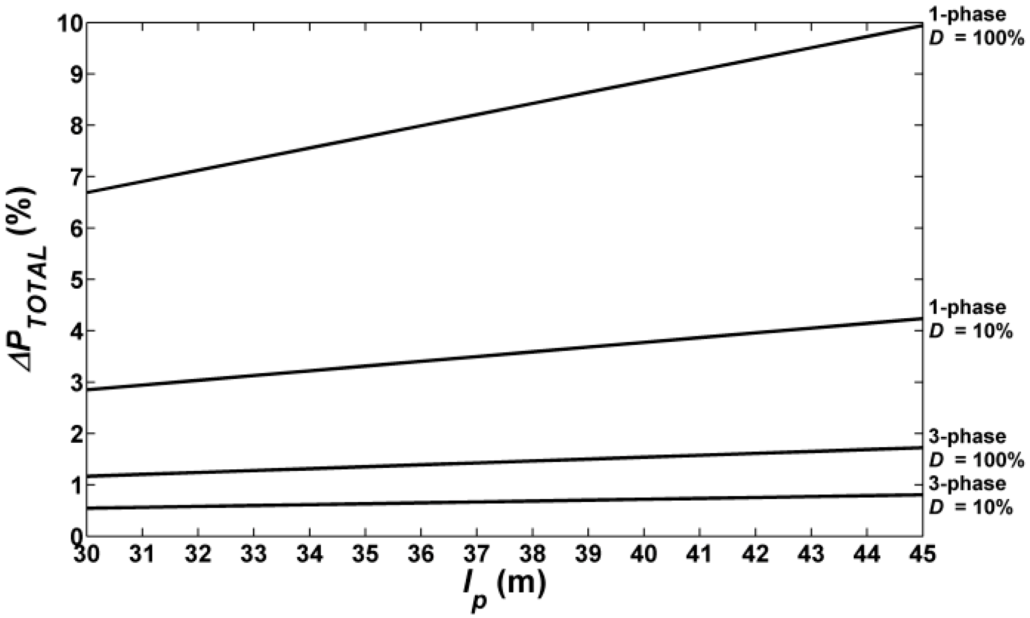
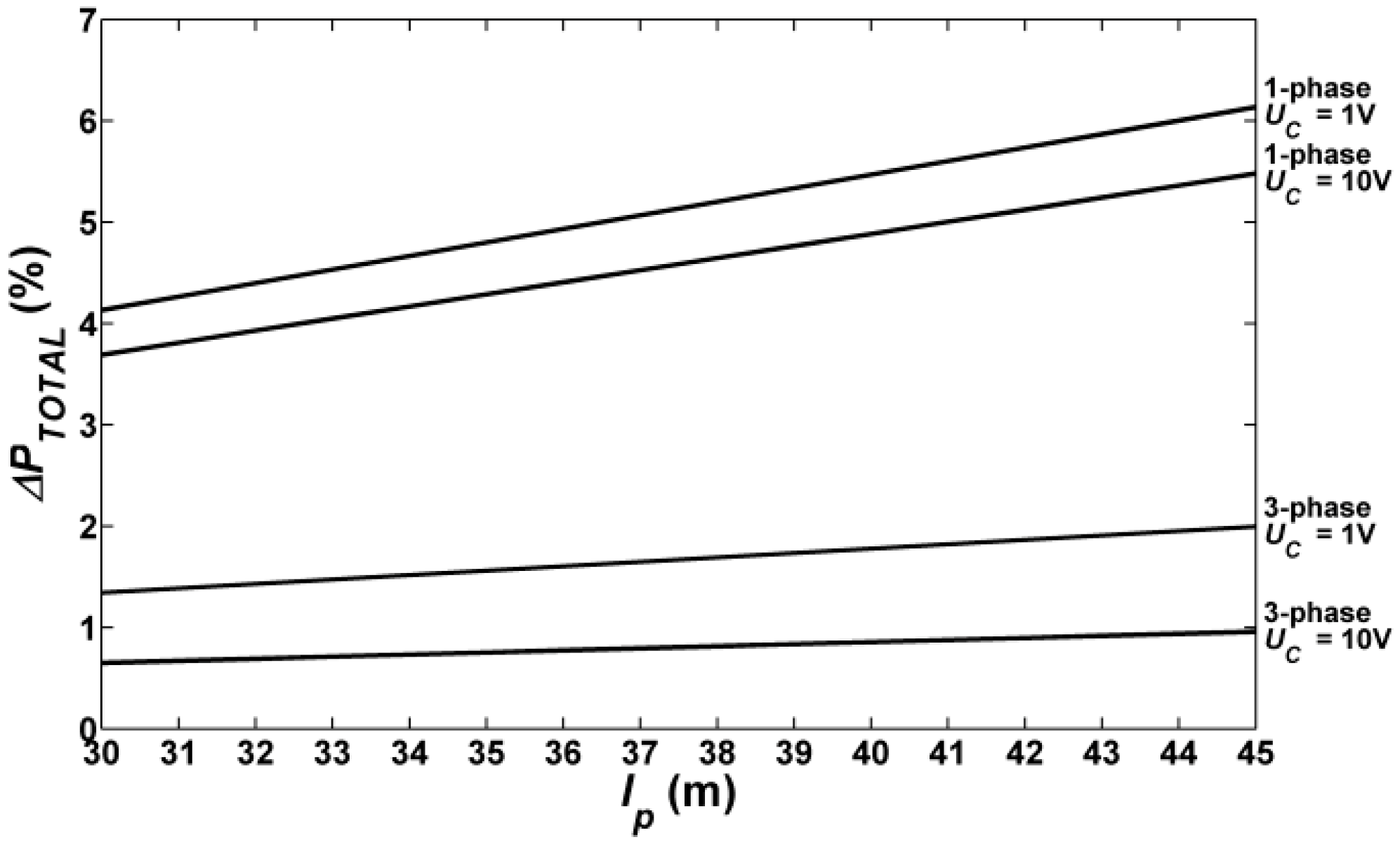
3.4. Estimation of Active Power Losses for Different Distances between Poles

The calculations presented in previous sections are made for a given distance between the poles reaching to 30 m. In practice, these distances may be different. It was considered interesting to estimate the effect of the distance between poles on the total losses of active power in the lighting installation. The range of the distance between poles from lp = 30 m to lp = 45 m was examined. Based on the calculations it can be stated that the dependence of the total power losses in the road lighting system depends linearly on the spacing of the poles.
Figure 8 and Figure 9 show the dependence of the percentage of total active power losses ΔPTOTAL in the road lighting system as a function of the distance between the poles, respectively for installations with three and 30 LUM1 luminaires. For a three-phase circuit, UC = 10 V and a circuit with three luminaires, these losses increase from 0.013% for lp = 30 m to 0.016% for lp = 45 m. When the dimming voltage is reduced to 1 V, the losses are greater and range from 0.016% for lp = 30 m to 0.019% for lp = 45 m. In a circuit composed of 30 luminaires, the percentages of power losses ΔPTOTAL at UC = 10 V increase from 0.386% (lp = 30 m) to 0.571% (lp = 45 m). With full dimming of these luminaires, ΔPTOTAL = 0.296% for the distance between the poles equal to 30 m. Increasing the distance between poles up to 45 m results in an increase in losses to 0.432%. In a single-phase system with LUM1 luminaires, the power losses are greater than in a three-phase system. When operating with a minimum dimming (UC = 1 V) and for a circuit with three luminaires, they are equal to 0.055% (lp = 30 m) and increase with increasing distance lp = 45 m to 0.068%. With full dimming (UC = 10 V), ΔPTOTAL ranges from 0.049% at lp = 30 m to 0.060% at lp = 45 m. For installations with 30 LUM1 luminaires operating with UC = 1 V, the calculated power losses for lp = 30 m and lp = 45 m are equal to 1.856% and 2.757% respectively. In the case of work with a full luminous flux, these losses are equal to 1.644% for lp = 30 m and 2.442% for lp = 45 m.
Considering the influence of changing the distance between columns for a lighting installation with LUM2 luminaires, similar dependencies are observed as for installations with LUM1 luminaires. With a dimming voltage equal to 2 V, the percentage of power losses ΔPTOTAL are higher than for the full-power luminaires (UC = 10 V). For a three-phase circuit with three luminaires, the power losses for this actuation range from 0.043% to 0.054% with the analyzed range of changes in the distance between the poles lp. After increasing the power of the luminaire to the maximum value (UC = 10 V), these losses are equal to 0.030% and 0.036% respectively. In a lighting installation with 30 LUM2 luminaires, the power losses ΔPTOTAL at UC = 2 V range from 1.341% to 1.994% for lp = 30 m and lp = 45 m. After increasing the power of luminaires (UC = 10 V), these losses for the analyzed range of changes lp are equal to 0.649% and 0.958%. In the case of a single-phase installation with three luminaires, the percentage losses ΔPTOTAL range from 0.122% to 0.152% for lp = 30 m and lp = 45 m and UC = 2 V. Increasing the power of luminaires to the maximum value caused that the percentage values of ΔPTOTAL are smaller and amount to 0.109% (lp = 30 m) and 0.152% (lp = 45 m). In an installation consisting of 30 LUM2 luminaires, the calculated power losses range from 4.130% to 6.135% for lp = 30 m and lp = 45 m and UC = 2 V, respectively. For UC = 10 V (with full dimming), these losses are equal to 3.689% and 5.480%. The dependencies of percentage power losses for installations with LUM2 luminaires are shown in Figure 10 and Figure 11.
The results of calculations of power losses for road lighting installations with three LUM3 luminaires as a function of distance between the poles are shown in Figure 12. The smallest percentage of power losses ΔPTOTAL occur for the three-phase installations and dimming D = 10%. They amount to 0.023% for lp = 30 m and increase to 0.028% for lp = 45 m. After changing the dimming, when D = 100%, these losses are between 0.052% and 0.063%. Increasing the number of luminaires results, of course, in the increase of power losses. For installations with 30 luminaires and D = 10%, they are equal to 0.546% (lp = 30 m) and 0.807% (lp = 45 m). Increasing the power of luminaires (D = 100%) results in an increase in power loss to 1.168% and 1.724% respectively. The calculated values of power losses ΔPTOTAL in the single-phase installation are much higher than in the three-phase system. They are for D = 10% and installations with three LUM3 luminaires, respectively, for lp = 30 m ΔPTOTAL = 0.082% and for lp = 45 m ΔPTOTAL = 0.103%. After increasing the power of luminaires to 100% of power, power losses increase to 0.193% and 0.241%. In an installation with 30 LUM3 luminaires (Figure 13), the percentages of ΔPTOTAL for the D = 10% dimming range from 2.850% to 4.236% for lp = 30 m and 45 m respectively. As can be expected, the increase in the power of luminaires (D = 100%) caused the losses increase up to 6.689% and 9.942%.
Summarizing the results of the calculations, it can be concluded that the dependence of active power losses on the distance between the poles, i.e., the length of the lighting circuit, is linear. For LUM1 and LUM2 luminaires, due to the increase in the value of generated higher harmonics current to the power network, the percentages of power losses are greater at the lowest possible dimming.

3.5. Analysis of the Effect of Luminaire Dimming and Active Power Losses on CO2 Emissions

In the Polish reality, electricity is generated mainly in thermal power plants fired with hard coal or lignite. The production of electricity is inherently associated with the emission of greenhouse gases, primarily CO2. The amount of CO2 emissions to the atmosphere depends on the amount of consumed electricity. In Poland, the guidelines contained in [22] are used to calculate CO2 emissions. The generation of 1 kWh of energy is accompanied by the emission of 0.781 kg of CO2. The analysis of the effect of dimming and active power losses on the level of CO2 emitted was made for road lighting installations with 30 luminaires, respectively LED1, LED2 and LED2. The results of the calculations are presented in Table 4. The calculations were made without taking into account active power losses in energy bill ( E Z CO 2 ), for the case of three-phase ( E 3 P CO 2 ) and single-phase ( E 1 P CO 2 ) installation, taking into account the power losses. The CO2 emission was determined for luminaires with full luminous flux and for the installation working in accordance with the assumed schedule. A graphical presentation of this schedule is shown in Figure 14. The times of switching on (ton) and off (toff) the luminaires were determined using astronomical tables of sunrises and sunsets for Poland. For simplicity, the mean values of these times were assumed for months. Based on these calculations, the annual lighting time of luminaires equals 3950 h. It was assumed that between hours 23 and 4, the luminaires may glow with a reduced value of luminous flux. D1 means the first level of dimming equals 100% and D2 is the second level. Calculations were made for whole available range of dimming for all considered luminaires.
For installations with luminaires with the lowest power of 32 W (LUM3), the value of CO2 emissions changes from 3.006 tons for variant—without dimming to 1.889 tons for dimming variant 1. For this case, the impact of active power losses on the CO2 emissions can be neglected. For installations with LUM2 luminaires, the value of CO2 emissions changes from 7.750 tons for without dimming variant to 4.895 tons for dimming variant 1. Analyzing the obtained results, it can be concluded that not taking into account active power losses causes underestimated emissions by several percent. For a three-phase system and without dimming variant, this underestimate is 0.05 tons and for a single-phase installation is 0.27 tons, respectively. The amount of CO2 emissions for road lighting installations with LUM3 luminaires varies from 13.370 tons for without dimming variant to 8.854 tons for dimming variant 1. The underestimation of CO2 emissions due to the omission of power losses for the considered installation may exceed 1% for a three-phase and 7% for a single-phase installation.

4. Discussion

In the preceding Sections the dependences which describe the losses of active power in the elements of the lighting network were depicted. For the specific configuration of the lighting circuit, power losses calculations were performed, and the losses dependence of the system parameters was analyzed. The analysis included the individual sources of losses irrespective of their share of the overall balance. Assumptions for this type of calculation in engineering practice can be ascribed initially to the accuracy (underestimation of up to 10%) and then selected for further analysis based merely on the components of the losses that are dominant. In this way, the calculation is simplified while preserving their accuracy. It has been assumed that the following factors have a decisive influence on the network losses: Level of luminaries dimming, network configuration (single or three phases) and number of light points.
With this assumption, total losses in the lighting system, as defined by the Equation (3), can be expressed as:
Δ P T O T A L = f ( k c o n f , k n , D ) .
Based on the calculations, it is assumed (Section 3 and Section 4) that the total losses from the single-phase and three-phase systems are virtually linear. The concept of a reduction coefficient kred, as the ratio of the power losses at the drive level to losses at full power was introduced as:
k r e d = Δ P T O T A L r e d Δ P T O T A L .
When the dimming characteristics of the luminaries are known (the relation of the active power of the luminaire to the degree of dimming), the reduction factor kred is the coefficient of slope of the dimming characteristic. The dependence of active power losses on the number of light points can be referred to two cases: One if the number of light points is ≤ 3 and second if the number of light points is >3. Total power losses for the three-phase network can be estimated from Equations (25) and (26).
Δ P T O T A L k r e d [ 3 l γ C S C [ n 2 ( l 01 + l l ) + n ( n 1 ) ( 2 n 1 ) 2 ] I L u m 2 + 2 l P W γ P W S P W I L u m 2 ] for n p 3 .
Δ P T O T A L k r e d 3 l γ C S C [ n 2 ( l 01 + l l ) + n ( n 1 ) ( 2 n 1 ) 2 ] I L u m 2 for n p > 3 .
In the case of single-phase networks, respectively:
Δ P T O T A L k r e d [ 2 l γ C S C [ n 2 ( l 01 l ) + n ( n 1 ) ( 2 n 1 ) 6 ] I L u m 2 + 2 l P W γ P W S P W I L u m 2 ] for n p 3 .
Δ P T O T A L k r e d 2 l γ C S C [ n 2 ( l 01 l ) + n ( n 1 ) ( 2 n 1 ) 6 ] I L u m 2 for n p > 3 .
The main components of active power losses are losses in the feeder wiring and in the wires in the pole. Power losses in the rest of the circuit are of lesser importance, but with low levels of dimming, and fewer luminaires, can have a significant impact. In the single-phase installations, the losses of active power are several times higher than in a three-phase installation, which can achieve values that, in the general balance of losses, are not to be ignored. On this basis, you can look for potential ways to reduce losses and thus improve the energy efficiency of the installation. The first stage of the design of a lighting installation is always a well-designed lighting project. Errors can be caused by the form of incorrect selection of lighting installation elements, for example - improper selection of luminaires are source of losses in the form of unjustified oversizing of installation elements or illumination of irrelevant areas. In this situation, even the best design and installation will not ensure the expected energy efficiency.
When calculating the electricity consumption of road lighting installations, power losses are usually neglected. As shown in this paper, this may cause a decrease in the value of CO2 emitted to the atmosphere by up to 7%. The same will also be the underestimation of electricity consumption, which in turn affects the economic efficiency (investment return time). If a single installation is considered, the effect of omitting active power losses seems to be inconsiderable. By overseeing such an analysis, for example for the entire city, the omission of power losses will underestimate the CO2 emissions calculated, even in tens of tons. In the opinion of the authors, power losses should be included in the calculations of energy efficiency and greenhouse gas emission levels. In particular, this applies to single-phase installations.

5. Conclusions

Active power losses occur at every electrical installation. The paper presents a detailed analysis of active power losses for the three-phase and single-phase road lighting systems. It describes a general dependence whereby total losses of active power can be determined, taking into account a certain number of luminaires and the level of dimming. These dependencies can be helpful in the design of road lighting installations and in calculating the energy efficiency of lighting installations. Typically, such projects are executed as multivariate, and the presented methods allow the right choice. The investment costs for the three-phase installation will always be higher than for the single-phase. Therefore, the selection of the installation (single- or three-phase) should be based on technical assumptions and economic analysis.

Author Contributions

Conceptualization, R.S., P.M. and W.P.; Data curation, R.S. and P.M.; Formal analysis, R.S. and P.M.; Methodology, R.S. and P.M.; Writing—original draft, R.S. and P.M.; Writing—review & editing, W.P.

Funding

This research received no external funding.

Conflicts of Interest

The authors declare no conflict of interest.

List of Variables

DPpower density indicator, (W/lx·m2)
PLSpower of the lighting system used to illuminate a specific area, (W)
Ēiaverage illumination density on the i-th surface of the specific area, (lx)
Aithe i-th area of the specific area that is illuminated by the lighting system, (m2)
nthe number of surfaces to be illuminated in particular area
Pkactive power of the k-th luminous point (light source, lamp device, and any other device such as a spot light dimming unit, switch or photocell, and the component associated with the luminous point and necessary for its operation), (W)
Padtotal active power of all devices not included in Pk but necessary to operate a road installation, such as a remote switch or photocell, centralized light dimming or centralized management system, etc. Total Pad power should be determined for the total number of luminaires in a lighting installation and determined in proportion to the number of luminaires in the specified area to be analyzed, (W)
nlunumber of lighting points (luminaires) in a lighting system in a specific area taken for analysis
PLumluminaire active power, (W)
QLumluminaire reactive power, (var)
PFDdisplacement power factor
PFDDdistorted power factor
THDIcurrent total harmonic distortion factor, (%)
tgϕtangens ϕ
ΦLumluminaire luminous flux, (lm)
ηLumluminaire luminous efficiency
ΔPTOTALtotal losses of active power, (W);
ΔPCABLElosses of active power in three (one) phase feeder wiring, (W);
ΔPNEUTRALlosses of active power in neutral conductor, (W);
ΔPWIRElosses of active power in wire in the pole, (W);
ΔPPPBlosses of active power in protection in the lighting panelboard, (W);
ΔPPPOLElosses of active power in protection in the pole, (W);
ΔPRELAYlosses of active power in relay, (W).
nnumber of luminaires per phase
l01distance of the first luminaire from the lighting switchboard, (m);
ldistance between poles, (m);
γCelectrical conductivity of feeder wiring, (m/Ωmm2);
SCcross-section of feeder wiring, (mm2);
ILumRMS value of luminaire current, (A);
IhLumzero sequence harmonic current for h = 3,9,15…, (A);
INLumRMS value of current flowing in the neutral conductor, (A).
lPWthe length of the wire that connects the pole switchboard to the luminaire, (m);
γPWelectrical conductivity of the wire connects the pole switchboard to the luminaire (m/Ωmm2);
SPWcross-section of the wire connecting the pole switchboard to the luminaire, (mm2);
RPWresistance of the wire connecting the pole switchboard to the luminaire, (Ω);
ILItotal current taken by the lighting installation, (A);
RPPBresistance of one phase of the safety device, (Ω).
RMCBresistance of miniature circuit breaker, (Ω).
RPBFBresistance of fuse carrier; (Ω);
RPBFresistance of fuse, (Ω).
ΔPPBFBactive power losses in fuse carrier for rated current; (W);
IPBFBrated current of fuse carrier, (A).
ΔPPBFactive power losses in fuse for rated current, (W);
IPBFrated current of fuse, (A).
RPPoleresistance of protection device, (Ω).
ΔPMCBrated active power losses of the miniature circuit breaker, (W)
IMCBrated current of the miniature circuit breaker, (A)
ΔPRELAYrated active power losses of the relay, (W)
RRresistance of the single phase of relay, (Ω).
IRrated current of relay, (A)
npnumber of lighting points (luminaires)
Pkccircuit power, (W)
Ddimming
kconffactor for network configuration (single-phase or three-phase);
knfactor taking into account the number of light points.
ΔPTOTALredtotal losses of active power during luminaire power reduction, (W)
kredthe reduction factor
E Z CO 2 CO2 emission without active power losses, (t)
E 3 P CO 2 CO2 emission with active power losses for three-phase installation, (t)
E 1 P CO 2 CO2 emission with active power losses for single-phase installation, (t)

Appendix A

Calculation results of three-phase road lighting installation.
Table A1. Relative percent of losses of active power in the lighting circuit elements referred to total losses ΔPTOTAL and the share of total losses ΔPTOTAL in active power per circuit for three luminaires of LUM1.
Dimming
UC (V)
ΔPCABLE
(%)
ΔPNEUTRAL
(%)
ΔPPBB
(%)
ΔPRELAY
(%)
ΔPWIRE
(%)
ΔPPPOLE
(%)
ΔPTOTAL
(W)
ΔPTOTAL/Pkc
(%)
1037.8851.2782.4382.38444.90011.1150.0030.013
937.8841.2792.4382.38444.90011.1150.0040.013
837.8951.2512.4382.38444.91311.1180.0040.013
737.8641.3332.4362.38244.87611.1090.0050.012
637.8501.3682.4352.38244.86011.1050.0060.011
537.8981.2442.4382.38444.91611.1190.0080.010
438.0240.9152.4472.39245.06611.1560.0100.009
337.1683.1452.3922.33944.05110.9050.0130.010
235.3547.8722.2752.22441.90110.3730.0130.014
135.9336.3642.3122.26142.58810.5430.0130.016
Table A2. Relative percent of losses of active power in the lighting circuit elements referred to total losses ΔPTOTAL and the share of total losses ΔPTOTAL in active power per circuit for 30 luminaires of LUM1.
Dimming
UC (V)
ΔPCABLE
(%)
ΔPNEUTRAL
(%)
ΔPPBB
(%)
ΔPRELAY
(%)
ΔPWIRE
(%)
ΔPPPOLE
(%)
ΔPTOTAL
(W)
ΔPTOTAL/Pkc
(%)
1091.2943.9441.1141.0892.0510.5082.8510.293
991.2923.9461.1141.0892.0510.5082.8510.293
891.3713.8631.1151.0902.0530.5082.8510.292
791.1394.1081.1121.0872.0480.5072.2760.268
691.0394.2131.1101.0862.0450.5061.7970.245
591.3923.8421.1151.0902.0530.5081.3850.223
492.3392.8451.1261.1012.0750.5141.0180.204
386.1709.3361.0511.0281.9360.4790.8590.223
274.78121.3190.9120.8921.6800.4160.9400.346
178.19317.7290.9540.9331.7570.4350.7260.386
Table A3. Relative percent of losses of active power in the lighting circuit elements referred to total losses ΔPTOTAL and the share of total losses ΔPTOTAL in active power per circuit for three luminaires of LUM2.
Dimming
UC (V)
ΔPCABLEΔPNEUTRALΔPPBBΔPRELAYΔPWIREΔPPPOLEΔPTOTALΔPTOTAL/Pkc
(%)(%)(%)(%)(%)(%)(W)(%)
1038.0240.9162.4472.39245.06511.1560.0750.030
938.0010.9772.4452.39145.03811.1490.0610.027
837.9511.1052.4422.38844.97911.1350.0480.024
737.9281.1652.4402.38644.95211.1280.0370.021
637.8641.3332.4362.38244.87611.1090.0280.019
537.7651.5912.4302.37644.75811.0800.0210.016
437.5692.1002.4172.36444.52711.0230.0140.014
337.4672.3662.4112.35744.40610.9930.0090.011
229.89422.1021.9231.88135.4308.7710.0220.043
Table A4. Relative percent of losses of active power in the lighting circuit elements referred to total losses ΔPTOTAL and the share of total losses ΔPTOTAL in active power per circuit for 30 luminaires of LUM2.
Dimming
UC (V)
ΔPCABLE
(%)
ΔPNEUTRAL
(%)
ΔPPBB
(%)
ΔPRELAY
(%)
ΔPWIRE
(%)
ΔPPPOLE
(%)
ΔPTOTAL
(W)
ΔPTOTAL/Pkc
(%)
1092.3362.8481.1261.1012.0750.51416.3080.649
992.1613.0321.1241.0992.0710.51313.2900.589
891.7913.4221.1201.0952.0620.51110.4770.526
791.6183.6041.1181.0932.0580.5108.1490.467
691.1404.1071.1121.0872.0480.5076.1520.410
590.4074.8781.1031.0782.0310.5034.5280.355
488.9896.3691.0851.0611.9990.4953.1040.302
388.2617.1361.0771.0531.9830.4912.0360.254
250.03247.3590.6100.5971.1240.2786.8281.341
Table A5. Relative percent of losses of active power in the lighting circuit elements referred to total losses ΔPTOTAL and the share of total losses ΔPTOTAL in active power per circuit for three luminaires of LUM3.
Dimming
(%)
ΔPCABLEΔPNEUTRALΔPPBBΔPRELAYΔPWIREΔPPPOLEΔPTOTALΔPTOTAL/Pkc
(%)(%)(%)(%)(%)(%)(W)(%)
10039.3510.7012.4022.34944.24410.9530.2270.052
9039.3500.7052.4022.34944.24310.9520.2000.049
8039.3290.7572.4012.34844.21910.9470.1750.046
7039.2990.8322.3992.34644.18610.9380.1510.043
6039.2630.9242.3972.34444.14510.9280.1240.039
5039.2171.0392.3942.34144.09410.9150.1000.035
4039.0511.4582.3842.33143.90710.8690.0780.032
3038.8991.8432.3742.32243.73510.8270.0590.029
2038.6222.5402.3582.30543.42510.7500.0370.024
1038.1363.7692.3282.27642.87710.6140.0270.023
Table A6. Relative percent of losses of active power in the lighting circuit elements referred to total losses ΔPTOTAL and the share of total losses ΔPTOTAL in active power per circuit for 30 luminaires of LUM3.
Dimming
(%)
ΔPCABLEΔPNEUTRALΔPPBBΔPRELAYΔPWIREΔPPPOLEΔPTOTALΔPTOTAL/Pkc
(%)(%)(%)(%)(%)(%)(W)(%)
10093.2582.1281.0791.0551.9880.49250.6081.168
9093.2482.1381.0791.0551.9880.49244.5751.092
8093.0992.2951.0771.0531.9840.49138.9841.024
7092.8852.5191.0751.0511.9800.49033.7820.964
6092.6252.7921.0721.0481.9740.48927.7860.874
5092.3033.1301.0681.0441.9670.48722.3770.792
4091.1344.3571.0551.0311.9420.48117.7000.727
3090.0785.4651.0421.0191.9200.47513.5050.670
2088.2077.4281.0210.9981.8800.4658.5610.559
1085.03410.7590.9840.9621.8120.4496.3580.546

Appendix B

Calculation results of single-phase road lighting installation.
Table A7. Relative percent of losses of active power in the lighting circuit elements referred to total losses ΔPTOTAL and the share of total losses ΔPTOTAL in active power per circuit for three luminaires of LUM1.
Dimming
UC (V)
ΔPCABLE
(%)
ΔPPBB
(%)
ΔPRELAY
(%)
ΔPWIRE
(%)
ΔPPPOLE
(%)
ΔPTOTAL
(W)
ΔPTOTAL/Pkc
(%)
1048.5562.0083.28236.9959.1580.0470.049
90.0470.049
80.0470.049
70.0380.044
60.0300.041
50.0230.037
40.0170.034
30.0130.035
20.0130.047
10.0100.055
Table A8. Relative percent of losses of active power in the lighting circuit elements referred to total losses ΔPTOTAL and the share of total losses ΔPTOTAL in active power per circuit for 30 luminaires of LUM1.
Dimming
UC (V)
ΔPCABLE
(%)
ΔPPBB
(%)
ΔPRELAY
(%)
ΔPWIRE
(%)
ΔPPPOLE
(%)
ΔPTOTAL
(W)
ΔPTOTAL/Pkc
(%)
1097.0680.5950.9711.0950.27116.0231.644
916.0231.644
816.0351.644
712.7701.501
610.0701.371
57.7941.256
45.7891.161
34.5551.182
24.3251.594
13.4961.856
Table A9. Relative percent of losses of active power in the lighting circuit elements referred to total losses ΔPTOTAL and the share of total losses ΔPTOTAL in active power per circuit for three luminaires of LUM2.
Dimming
UC (V)
ΔPCABLE
(%)
ΔPPBB
(%)
ΔPRELAY
(%)
ΔPWIRE
(%)
ΔPPPOLE
(%)
ΔPTOTAL
(W)
ΔPTOTAL/Pkc
(%)
1048.5562.0083.28236.9959.1580.2740.109
90.2230.099
80.1750.088
70.1360.078
60.1020.068
50.0750.059
40.0500.049
30.0330.041
20.0620.122
Table A10. Relative percent of losses of active power in the lighting circuit elements referred to total losses ΔPTOTAL and the share of total losses ΔPTOTAL in active power per circuit for 30 luminaires of LUM2.
Dimming
UC (V)
ΔPCABLE
(%)
ΔPPBB
(%)
ΔPRELAY
(%)
ΔPWIRE
(%)
ΔPPPOLE
(%)
ΔPTOTAL
(W)
ΔPTOTAL/Pkc
(%)
1097.0680.5950.9711.0950.27192.6873.689
975.3893.342
859.1952.971
745.9552.635
634.5142.299
525.1991.978
417.0001.651
311.0591.378
221.0264.130
Table A11. Relative percent of losses of active power in the lighting circuit elements referred to total losses ΔPTOTAL and the share of total losses ΔPTOTAL in active power per circuit for three luminaires of LUM3.
Dimming
(%)
ΔPCABLE
(%)
ΔPPBB
(%)
ΔPRELAY
(%)
ΔPWIRE
(%)
ΔPPPOLE
(%)
ΔPTOTAL
(W)
ΔPTOTAL/Pkc
(%)
10049.9621.7843.20336.1128.9400.8360.193
900.7360.180
800.6430.169
700.5560.159
600.4560.143
500.3660.129
400.2860.117
300.2150.107
200.1340.087
100.0960.082
Table A12. Relative percent of losses of active power in the lighting circuit elements referred to total losses ΔPTOTAL and the share of total losses ΔPTOTAL in active power per circuit for three luminaires of LUM3.
Dimming
(%)
ΔPCABLEΔPPBBΔPRELAYΔPWIREΔPPPOLEΔPTOTALΔPTOTAL/Pkc
(%)(%)(%)(%)(%)(W)(%)
10097.2640.5140.9231.0410.258289.9146.689
90255.3306.256
80222.9425.857
70192.7505.501
60158.0984.974
50126.8764.492
4099.0854.071
3074.7263.705
2046.3863.029
1033.2112.850

References

  1. Queiroz, L.M.O.; Roselli, M.A.; Cavellucci, C.; Lyra, C. Energy Losses Estimation in Power Distribution Systems. IEEE Trans. Power Syst. 2012, 27, 1879–1887. [Google Scholar] [CrossRef]
  2. Sun, D.I.H.; Abe, S.; Shoults, R.R.; Chen, M.S.; Eichenberger, P.; Farris, D. Calculation of energy losses in a distribution system. IEEE Trans. Power Appar. Syst. 1980, PAS-99, 1347–1356. [Google Scholar] [CrossRef]
  3. Stojkov, M.; Nikolovski, S. Technical losses in power distribution network. In Proceedings of the IEEE MELECON, Benalmádena (Málaga), Spain, 16–19 May 2006. [Google Scholar]
  4. Gabryjelski, Z.; Kowalski, Z. Sieci i Urządzenia Oświetleniowe. Zagadnienie Wybrane; Wydawnictwo Politechniki Łódzkiej: Łódź, Poland, 1997; ISBN 83-86453-95-8. [Google Scholar]
  5. Lobão, J.A.; Devezas, T.; Catalão, J.P.S. Influence of cable losses on the economic analysis of efficient and sustainable electrical equipment. Energy 2014, 65, 145–151. [Google Scholar] [CrossRef]
  6. Vysotsky, V.S.; Nosov, A.A.; Fetisov, S.S.; Shutov, K.A. AC Loss and Other Researches with 5 m HTS Model Cables. IEEE Trans. Appl. Superconduct. 2011, 21, 1001–1004. [Google Scholar] [CrossRef]
  7. Pinto, M.F.; Soares, G.M.; Mendonça, T.R.F.; Almeida, P.S.; Braga, H.A.C. Smart Modules for Lighting. In Proceedings of the 2014 11th IEEE/IAS International Conference on Industry Applications, Juiz de For a, Brazil, 7–10 December 2014. [Google Scholar]
  8. Todorović, B.M.; Samardžija, D. Road lighting energy-saving system based on wireless sensor network. Energy Effic. 2017, 10, 239–247. [Google Scholar] [CrossRef]
  9. Bielecki, S.; Skoczkowski, T. An enhanced concept of Q-power management. Energy 2018, 162, 335–353. [Google Scholar] [CrossRef]
  10. Mekhamer, S.F.; El-Hawary, M.E.; Soliman, S.A.; Moustafa, M.A.; Mansour, M.M. New Heuristic Strategies for Reactive Power Compensation of Radial Distribution Feeders. IEEE Trans. Power Deliv. 2002, 17, 1128–1135. [Google Scholar] [CrossRef]
  11. Yan, W.; Hui, S.Y.R.; Shu-Hung Chung, H. Energy Saving of Large-Scale High-Intensity-Discharge Lamp Lighting Networks Using a Central Reactive Power Dimming System. IEEE Trans. Ind. Electron. 2009, 56, 3069–3078. [Google Scholar] [CrossRef]
  12. Ożadowicz, A.; Grela, J. Energy saving in the street lighting dimming system—A new approach based on the EN-15232 standard. Energy Effic. 2017, 10, 563–576. [Google Scholar] [CrossRef]
  13. Radulovic, D.; Skok, S.; Kirincic, V. Energy efficiency public lighting management in the cities. Energy 2011, 36, 1908–1915. [Google Scholar] [CrossRef]
  14. Gutierrez-Escolar, A.; Castillo-Martinez, A.; Gomez-Pulido, J.M.; Gutierrez-Martinez, J.M.; Dominguez González-Seco, E.P.; Stapic, Z. A review of energy efficiency label of street lighting systems. Energy Effic. 2017, 10, 265–282. [Google Scholar] [CrossRef]
  15. Pracki, P. A proposal to classify road lighting energy efficiency. Light. Res. Technol. 2011, 43, 271–280. [Google Scholar] [CrossRef]
  16. Kostic, M.; Djokic, L. Recommendations for energy efficient and visually acceptable street lighting. Energy 2009, 34, 1565–1572. [Google Scholar] [CrossRef]
  17. Kovacs, A.; Batai, R.; Csanad Csaji, B.; Dudas, P.; Hay, B.; Pedone, G.; Revesz, T.; Vancza, J. Intelligent dimming for energy-positive street lighting. Energy 2016, 114, 40–51. [Google Scholar] [CrossRef]
  18. Lv, F.; Wang, Z.; Ding, Y.; Li, Y.; Zhu, N. A systematic method for evaluating the effects of efficient lighting project in China. Energy Effic. 2016, 9, 1037–1052. [Google Scholar] [CrossRef]
  19. PN-EN 13201:2016. Oświetlenie dróg. PEPiREE. 2017. Available online: http://oswietlenie.ptpiree.pl/konferencje/oswietlenie-15/2017/32_www_m_gorczewska.pdf (accessed on 11 December 2018).
  20. IEEE Std. 1459-2010. Definitions for the Measurement of Electric Power Quantities Under Sinusoidal, Nonsunusoidal, Balanced, or Unbalanced Conditions; IEEE: New Jersey, NJ, USA, 2010. [Google Scholar]
  21. Jettanasen, C.; Pothisarn, C. Analytical Study of Harmonics Issued from LED Lamp Driver. In Proceedings of the International MultiConference of Engineers and Computer Scientists, IMECS 2014, Hong Kong, China, 12–14 March 2014; Volume II. [Google Scholar]
  22. Krajowy Ośrodek Bilansowania i Zarządzania Emisjami. Wskaźniki Emisyjności CO2, SO2, NOx, CO i pyłu Całkowitego DLA Energii Elektrycznej. Available online: http://www.kobize.pl/ (accessed on 12 December 2018).
Figure 1. Example of a road lighting installation.
Sustainability 10 04742 g001
Figure 2. Dependence of total active power losses ΔPTOTAL in relation to the dimming and the number of poles np for LUM1.
Sustainability 10 04742 g002
Figure 3. Dependence of total active power losses ΔPTOTAL in relation to the dimming and the number of poles np for LUM2.
Sustainability 10 04742 g003
Figure 4. Dependence of total active power losses ΔPTOTAL in relation to the dimming and the number of poles np for LUM3.
Sustainability 10 04742 g004
Figure 5. Dependence of total active power losses ΔPTOTAL in relation to the dimming and the number of poles np for LUM1.
Sustainability 10 04742 g005
Figure 6. Dependence of total active power losses ΔPTOTAL in relation to the dimming and the number of poles np for LUM2.
Sustainability 10 04742 g006
Figure 7. Dependence of total active power losses ΔPTOTAL in relation to the dimming and the number of poles np for LUM3.
Sustainability 10 04742 g007
Figure 8. Relative total power losses in relation to the distance between poles for circuit consisting of three luminaires for LUM1.
Sustainability 10 04742 g008
Figure 9. Relative total power losses in relation to the distance between poles for circuit consisting of 30 luminaires for LUM1.
Sustainability 10 04742 g009
Figure 10. Relative total power losses in relation to the distance between poles for circuit consisting of three luminaires for LUM2.
Sustainability 10 04742 g010
Figure 11. Relative total power losses in relation to the distance between poles for circuit consisting of 30 luminaires for LUM2.
Sustainability 10 04742 g011
Figure 12. Relative total power losses in relation to the distance between poles for circuit consisting of three luminaires for LUM3.
Sustainability 10 04742 g012
Figure 13. Relative total power losses in relation to the distance between poles for circuit consisting of 30 luminaires for LUM3.
Sustainability 10 04742 g013
Figure 14. Work schedule accepted for calculation.
Sustainability 10 04742 g014
Table 1. Values of electrical and photometric parameters for various levels of dimming of LUM1 luminaires.
Dimming
UC (V)
Plum
(W)
Qlum
(var)
PFD
(-)
tgϕ
(-)
PFDD
(-)
THDI
(%)
Φ
(lm)
ηLum
(lm/W)
1032.48314.7910.9100.4550.90113.917273684.238
932.48314.7930.9100.4550.90113.893273684.238
832.50914.7760.9100.4550.90213.854273684.161
728.35614.4780.8910.5110.88114.427240984.941
624.48014.1100.8660.5760.85714.903207284.635
520.67713.7880.8320.6670.82215.013174784.643
416.624134960.7760.8120.76715.130138883.505
312.84513.6420.6861.0620.66822.199100177.918
29.04515.0010.5161.6580.48336.87362168.571
16.27714.0310.4082.2350.37338.00739362.510
Table 2. Values of electrical and photometric parameters for various levels of dimming of LUM2 luminaires.
Dimming
UC (V)
Plum
(W)
Qlum
(var)
PFD
(-)
tgϕ
(-)
PFDD
(-)
THDI
(%)
Φ
(lm)
ηLum
(lm/W)
1083.74417.8700.9780.2130.96613.31912,011143.432
975.19417.1970.9750.2290.96213.71610,941145.511
866.41915.4500.9740.2330.95914.7159831148.013
758.13814.5180.9700.2500.95315.5578705149.725
650.04613.1130.9670.2620.94616.6117553150.909
542.46211.5390.9650.2720.94017.7486361149.812
434.31310.2550.9580.2990.92419.5925139149.781
326.7529.5840.9410.3580.89322.8143956,147.888
216.9695.9580.9440.3510.411202.0602789164.349
Table 3. Values of electrical and photometric parameters for various levels of dimming of LUM3 luminaires.
DimmingPlum
(W)
Qlum
(var)
PFD
(-)
tgϕ
(-)
PFDD
(-)
THDI
(%)
Φ
(lm)
ηLum
(lm/W)
100%144.47036.6560.9690.2590.9558.00314,08197.467
90%136.04036.3220.9660.2740.9518.45313,39098.427
80%126.89036.2350.9620.2940.9459.14612,66499.803
70%116.79036.0030.9560.3180.9379.82311,870101.635
60%105.94035.3920.9480.3470.92910.41710,980103.644
50%94.15233.9460.9410.3770.91911.0059971105.903
40%81.12932.5370.9280.4240.90412.3368804108.519
30%67.23332.4300.9010.5240.87114.3387437110.615
20%51.05030.4950.8580.6800.82316.8385859114.770
10%38.84328.9130.8020.9210.75921.0524579117.885
Table 4. Calculated CO2 emission.
LuminaireDimming VariantCO2 Emission
(t)
E Z CO 2 E 3 P CO 2 E 1 P CO 2
LUM1Without dimmingD1 = 10 V3.0063.0123.040
Diming variant 7D1 = 10 V, D2 = 7 V2.8302.8352.860
Diming variant 6D1 = 10 V, D2 = 6 V2.6642.6692.692
Diming variant 5D1 = 10 V, D2 = 5 V2.5012.5062.537
Diming variant 4D1 = 10 V, D2 = 4 V2.3282.3322.352
Diming variant 3D1 = 10 V, D2 = 3 V2.1672.1712.189
Diming variant 2D1 = 10 V, D2 = 2 V2.0042.0082.026
Diming variant 1D1 = 10 V, D2 = 1 V1.8861.8901.907
LUM2Without dimmingD1 = 10 V7.7507.7988.018
Diming variant 8D1 = 10 V, D2 = 9 V7.3857.4287.630
Diming variant 7D1 = 10 V, D2 = 8 V7.0107.0497.233
Diming variant 6D1 = 10 V, D2 = 7 V6.6566.6926.861
Diming variant 5D1 = 10 V, D2 = 6 V6.3106.3436.500
Diming variant 4D1 = 10 V, D2 = 5 V5.9856.0176.163
Diming variant 3D1 = 10 V, D2 = 4 V5.6375.6665.804
Diming variant 2D1 = 10 V, D2 = 3 V5.3135.3425.472
Diming variant 1D1 = 10 V, D2 = 2 V4.8954.9305.067
LUM3Without dimmingD1 = 100%13.37013.54314.358
Diming variant 9D1 = 100%, D2 = 90%13.01013.17313.943
Diming variant 8D1 = 100%, D2 = 80%12.61912.77313.501
Diming variant 7D1 = 100%, D2 = 70%12.18712.33213.021
Diming variant 6D1 = 100%, D2 = 60%11.72311.85912.503
Diming variant 5D1 = 100%, D2 = 50%11.21911.34711.950
Diming variant 4D1 = 100%, D2 = 40%10.66210.78211.349
Diming variant 3D1 = 100%, D2 = 30%10.06810.18210.716
Diming variant 2D1 = 100%, D2 = 20%9.3769.4829.980
Diming variant 1D1 = 100%, D2 = 10%8.8548.9569.437

