Improving Environmental Sustainability by Characterizing Spatial and Temporal Concentrations of Ozone

Abstract
1. Introduction
2. Materials and Methods
2.1. Data
2.2. Methodology
2.2.1. k-Means Clustering Algorithm
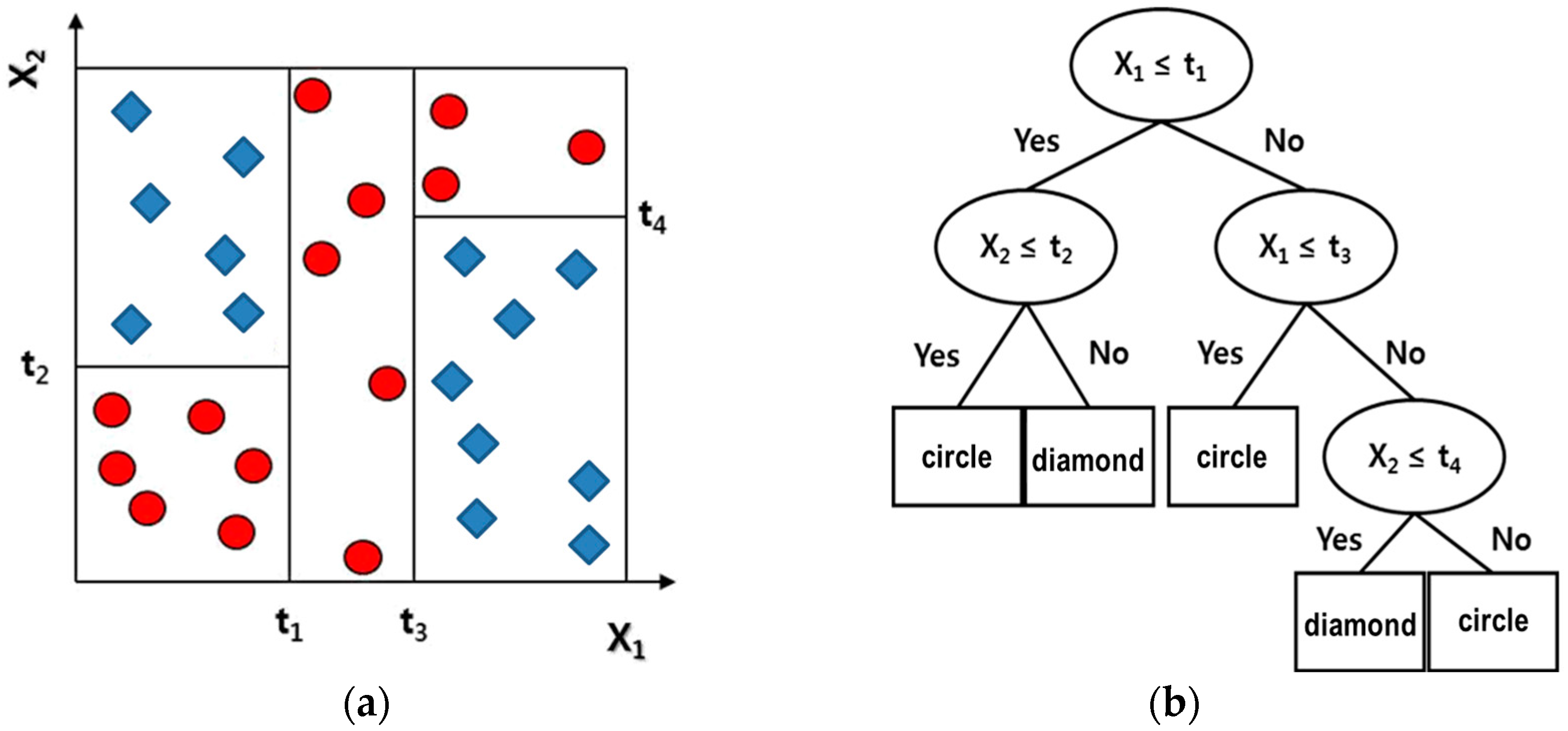
2.2.2. Decision Tree Algorithm
3. Results and Discussion
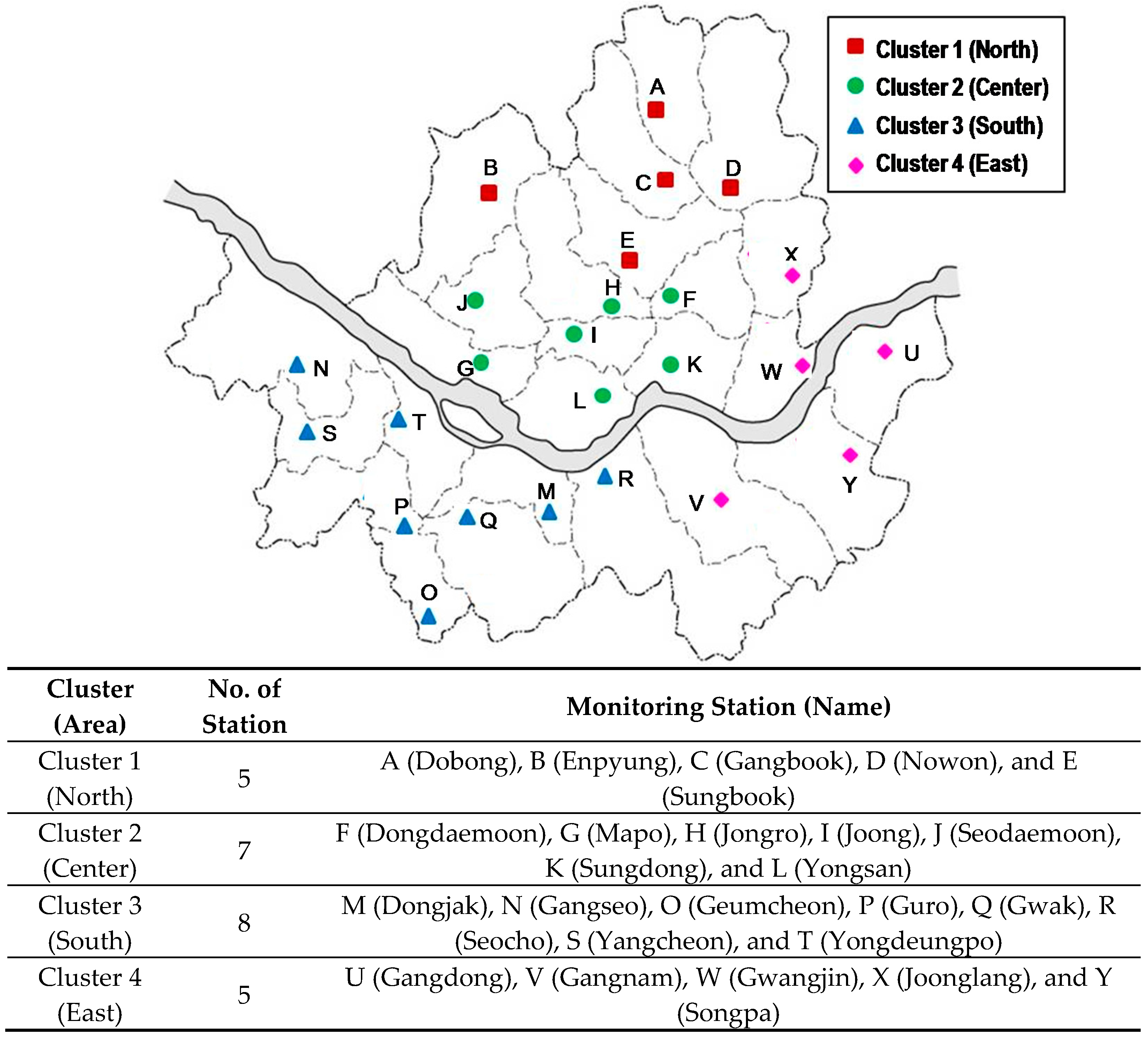
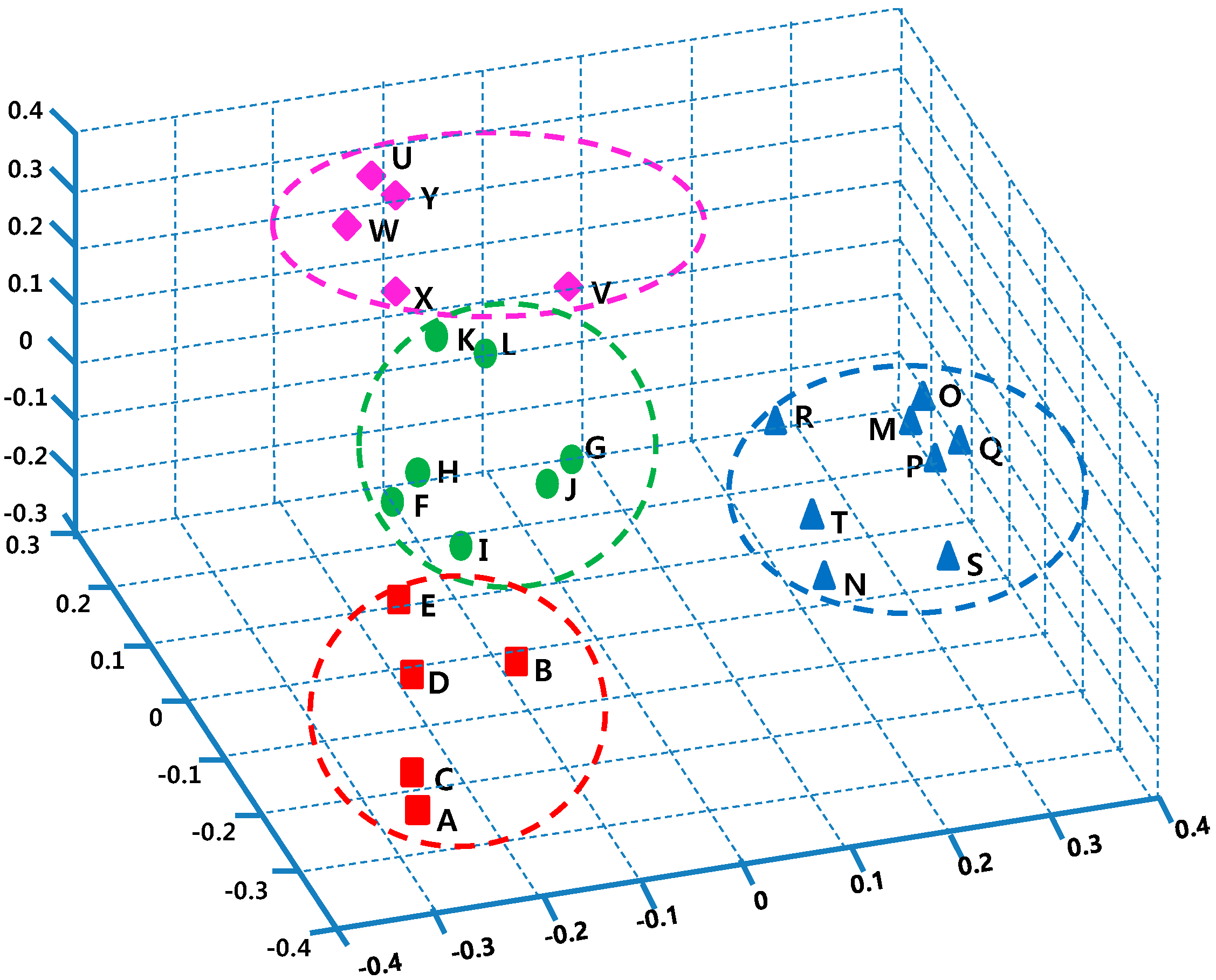
3.1. Spatial Characteristics of Ozone Concentrations
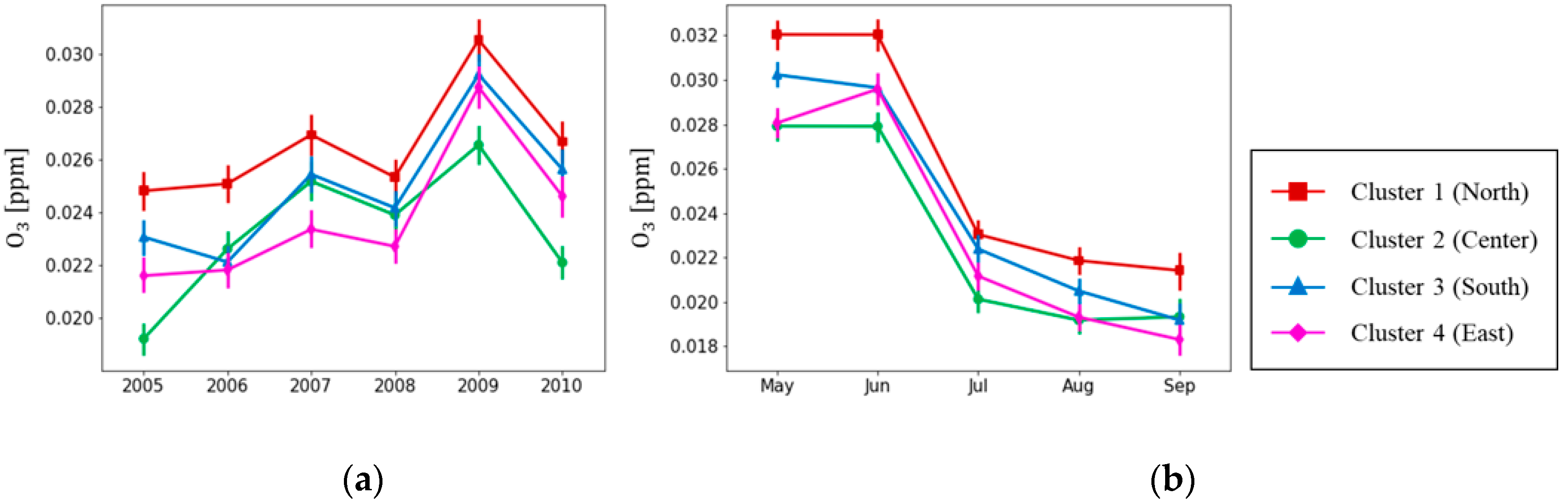
3.2. Temporal Patterns of Ozone Concentrations
3.3. Factors Determining High Ozone Concentrations
4. Conclusions
Author Contributions
Funding
Conflicts of Interest
References
- Oh, I.B.; Kim, Y.K.; Hwang, M.K. Ozone Pollution Patterns and the Relation to Meteorological Conditions in the Greater Seoul Area. J. Korean Soc. Atmos. Environ. 2005, 21, 357–365. [Google Scholar]
- Carrol, R.J.; Chen, R.; George, E.I.; Li, T.H.; Newton, J.; Schmiediche, H.; Wang, N. Ozone Exposure and Population Density in Harris County, Texas. J. Am. Statist. Assoc. 1997, 92, 392–404. [Google Scholar] [CrossRef]
- Felzer, B.S.; Cronin, T.; Reily, J.M.; Melillo, J.M.; Wang, X. Impacts of Ozone on Trees and Crops. C. R. Geosci. 2016, 339, 784–798. [Google Scholar] [CrossRef]
- Fuhrer, J.; Martin, M.; Mills, G.; Heald, C.; Harmens, H.; Hayes, F.; Sharps, K.; Bender, J.; Ashmore, M. Current and future ozone risks to global terrestrial biodiversity and ecosystem processes. Ecol. Evol. 2016, 6, 8785–8799. [Google Scholar] [CrossRef] [PubMed]
- Huerta, G.; Sansó, B.; Stroud, J.R. A Spatiotemporal Model for Mexico City Ozone Levels. J. R. Stat. Soc. Ser. C Appl. Stat. 2004, 53, 231–248. [Google Scholar] [CrossRef]
- Lee, H.J. Analysis of Time Series Models for Ozone at the Southern Part of Gyeonggi-do in Korea. J. Korean Soc. Atmos. Environ. 2007, 23, 364–372. [Google Scholar] [CrossRef]
- Bauer, G.; Deistler, M.; Scherrer, W. Time Series Models for Short Term Forecasting of Ozone in the Eastern Part of Austria. Environmetrics 2001, 12, 117–130. [Google Scholar] [CrossRef]
- El-Tahan, M. Temporal and Spatial Ozone Distribution over Eqypt. Climate 2018, 6, 1–15. [Google Scholar]
- Abdul-Wahab, S.A.; Bakheit, C.S.; Al-Alawi, S.M. Principal Component and Multiple Regression Analysis in Modelling of Ground-Level Ozone and Factors Affecting its Concentrations. Environ. Modell. Softw. 2005, 20, 1263–1271. [Google Scholar] [CrossRef]
- Cannistraro, G.; Cannistraro, M.; Cannistraro, A.; Galvagno, A. Analysis of Air Pollution in the Urban Center of Four Cities Sicilian. Int. J. Heat Technol. 2016, 34, S219–S225. [Google Scholar] [CrossRef]
- Sousa, S.I.V.; Martins, F.G.; Alvim-Ferraz, M.C.M.; Pereira, M.C. Multiple Linear Regression and Artificial Neural Networks Based on Principal Components to Predict Ozone Concentrations. Environ. Modell. Softw. 2007, 22, 97–103. [Google Scholar] [CrossRef]
- Kim, Y.G.; Lee, C.B. Development of Neural Network Model for Prediction of Daily Maximum Ozone Concentrations in Summer. J. Korean Soc. Atmos. Environ. 1984, 10, 224–232. [Google Scholar]
- Jorquera, H.; Pérez, R.; Cipriano, A.; Espejo, A.; Letelier, M.V.; Acuna, G. Forecasting Ozone Daily Maximum Levels at Santiago, Chile. Atmos. Environ. 1998, 32, 3415–3424. [Google Scholar] [CrossRef]
- Cannistraro, M.; Lorenzini, E. The Application of the New Technologies “E-Sensing” in Hospitals. IJM T 2016, 34, 551–557. [Google Scholar] [CrossRef]
- Kim, Y.J. A Study on the Development of Operable Models Predicting Tomorrow’s Maximum Hourly Concentrations of Air Pollutants in Seoul. J. Korean Soc. Atmos. Environ. 1997, 13, 79–89. [Google Scholar]
- Kim, Y.K.; Sohn, K.T.; Moon, Y.S.; Oh, I.B. Development of Transfer Function Model to Frecased Ground-level Concentration in Seoul. J. Korean Soc. Atmos. Environ. 1999, 15, 779–789. [Google Scholar]
- Kim, S.B.; Temiyasathit, C.; Chen, V.C.P.; Park, S.K.; Sattler, M.; Russell, A.G. Characterization of Spatially Homogeneous Regions Based on Temporal Patterns of Fine Particulate Matter in the Continental United States. J. Air Waste Manag. Assoc. 2008, 58, 965–975. [Google Scholar] [CrossRef]
- Yoo, E.C.; Park, O.H. The Assessment of Air Quality Monitoring Network Considering the Change of various Environmental Factors in Busan. J. Korean Soc. Atmos. Environ. 2006, 22, 405–420. [Google Scholar]
- Korea Environment Corporation. Air Quality and Environment Management. Available online: https://www.keco.or.kr/en/core/climate_air1/contentsid/1946/index.do (assessed on 11 January 2018).
- Ministry of Environment. Operational Guideline of Air Pollution Monitoring System; Ministry of Environment: Sejong City, Korea, 2016; NIER-GP2016-086.
- Le, N.D.; Zidek, J.V. Statistical Analysis of Environmental Space-Time Processes; Springer Science and Business Media: Berlin, Germany, 2006. [Google Scholar]
- The R Project for Statistical Computing. Available online: https://www.r-project.org/ (accessed on 12 February 2018).
- Gordon, A.D. Classification; Chapman and Hall/CRC: Boca Raton, FL, USA, 1999. [Google Scholar]
- Lee, K.J.; Kim, S.B.; Park, S. Daily, Seasonal, and Spatial Patterns of PM10 in Seoul, Korea. In Proceedings of the International Symposium on System Informatics and Engineering, Qingdao, China, 11–13 July 2011. [Google Scholar]
- Tan, P.; Steinbach, M.; Kumar, V. Introduction to Data Mining, 2nd ed.; Pearson Addison-Wesley: Boston, MA, USA, 2016. [Google Scholar]
- Roweis, S.T.; Saul, L.K. Nonlinear Dimensionality Reduction by Locally Linear Embedding. Science 2000, 290, 2323–2326. [Google Scholar] [CrossRef]
- Moon, S.S.; Kang, S.; Jitpitaklert, W.; Kim, S.B. Decision Tree Models for Characterizing Smoking Patterns of Older Adults. Expert Syst. Appl. 2012, 39, 445–451. [Google Scholar] [CrossRef]
- Breiman, L. Classification and Regression Trees, 1st ed.; Routledge: Abingdon, UK, 2017. [Google Scholar]
- CADDIS Volume 4: Data Analysis. Classification and Regression Tree (CART) Analysis. Available online: https://www.epa.gov/caddis-vol4/ (accessed on 10 February 2018).
- What’s CAI. Available online: https://www.airkorea.or.kr/eng/cai/cai1 (accessed on 7 February 2018).
- Wang, Y.; Xin, Q.; Coenen, F. A Novel Rule Ordering Approach in Classification Association Rule Mining. In Machine Learning and Data Mining in Pattern Recognition; Lecture Notes in Computer Science; Perner, P., Ed.; Springer: Berling/Heidelberg, Germany, 2007; Volume 4571, pp. 339–348. [Google Scholar]
- Kim, S.; Yoon, S.; Won, J.; Choi, S. Ground-based Remote Sensing Measurements of Aerosol and Ozone in an Urban Area: A Case Study of Mixing Height Evolution and its Effect on Ground-level Ozone Concentrations. Atmos. Environ. 2007, 41, 7069–7081. [Google Scholar] [CrossRef]
- Chu, H.; Lin, C.; Liau, C.; Kuo, Y. Identifying Controlling Factors of Ground-level Ozone Levels over Southwestern Taiwan using a Decision Tree. Atmos. Environ. 2012, 60, 142–152. [Google Scholar] [CrossRef]
- Park, S. Assessing Factors Linked with Ozone Exceedances in Seoul, Korea through a Decision Tree Algorithm. J. Environ. Sci. Int. 2016, 25, 191–216. [Google Scholar] [CrossRef]


| Source | DF | SS | MS | F | p-value |
|---|---|---|---|---|---|
| Factor | 3 | 0.7064 | 0.2355 | 538.69 | 0 |
| Error | 496,796 | 217.1545 | 0.0004 | ||
| Total | 496,799 | 217.8609 |
| Month | No. of Exceeding 1 h Standard | No. of Issuing Ozone Warning |
|---|---|---|
| May | 315 | 27 |
| June | 1077 | 280 |
| July | 549 | 125 |
| August | 487 | 148 |
| September | 69 | 7 |
| Region | Rule |
|---|---|
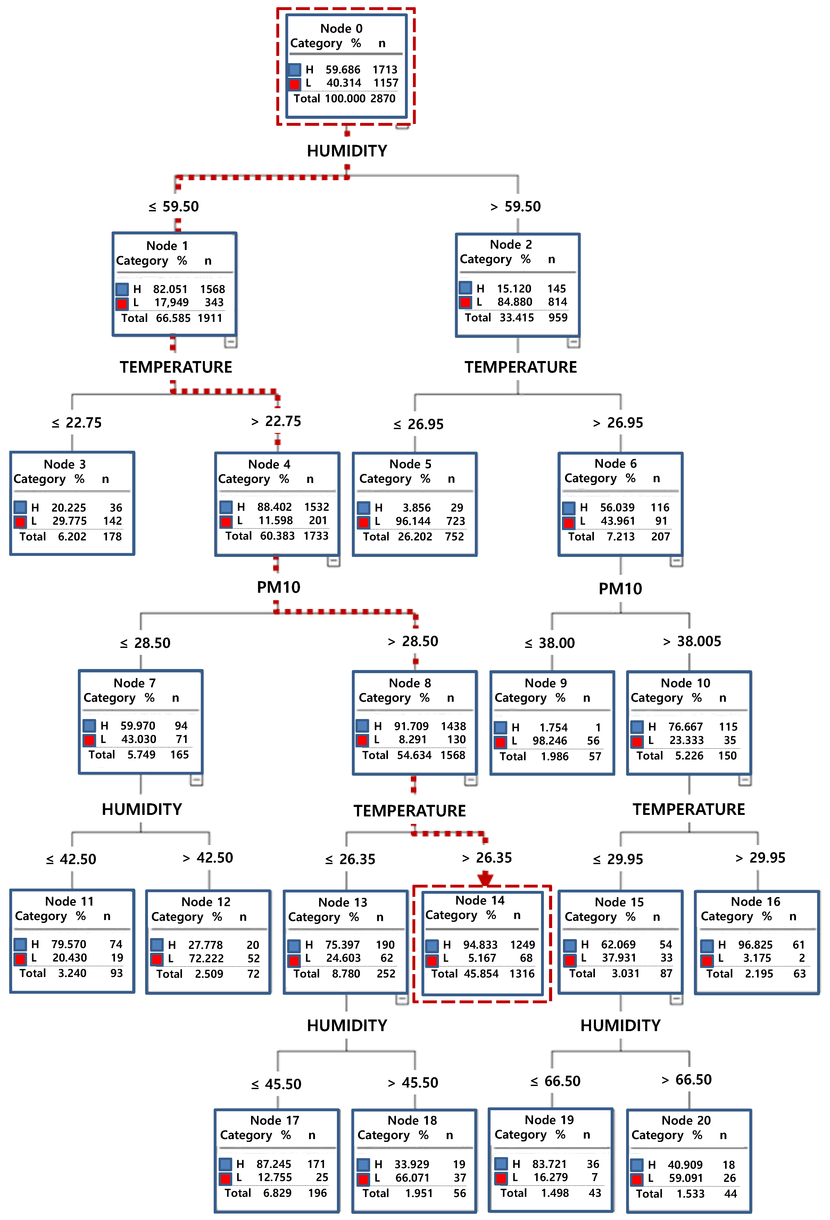
| Overall Seoul | PM10 ≥ 29.5 μg·m–3, Temperature ≥ 25.05 °C, Relative Humidity ≤ 60.5% |
| North | PM10 ≥ 28.5 μg·m–3, Temperature ≥ 26.35 °C, Relative Humidity ≤ 59.5% |
| Center | PM10 ≥ 41.5 μg·m–3, Temperature ≥ 26.05 °C, Relative Humidity ≤ 65.5% |
| South | PM10 ≥ 45.5 μg·m–3, Temperature ≥ 26.75 °C, Relative Humidity ≤ 60.5% |
| East | PM10 ≥ 36.5 μg·m–3, Temperature ≥ 26.35 °C, Relative Humidity ≤ 58.5% |
© 2018 by the authors. Licensee MDPI, Basel, Switzerland. This article is an open access article distributed under the terms and conditions of the Creative Commons Attribution (CC BY) license (http://creativecommons.org/licenses/by/4.0/).
Share and Cite
Lee, K.J.; Kahng, H.; Kim, S.B.; Park, S.K. Improving Environmental Sustainability by Characterizing Spatial and Temporal Concentrations of Ozone. Sustainability 2018, 10, 4551. https://doi.org/10.3390/su10124551
Lee KJ, Kahng H, Kim SB, Park SK. Improving Environmental Sustainability by Characterizing Spatial and Temporal Concentrations of Ozone. Sustainability. 2018; 10(12):4551. https://doi.org/10.3390/su10124551
Chicago/Turabian StyleLee, Kyu Jong, Hyungu Kahng, Seoung Bum Kim, and Sun Kyoung Park. 2018. "Improving Environmental Sustainability by Characterizing Spatial and Temporal Concentrations of Ozone" Sustainability 10, no. 12: 4551. https://doi.org/10.3390/su10124551
APA StyleLee, K. J., Kahng, H., Kim, S. B., & Park, S. K. (2018). Improving Environmental Sustainability by Characterizing Spatial and Temporal Concentrations of Ozone. Sustainability, 10(12), 4551. https://doi.org/10.3390/su10124551