Spatial Effects of Public Service Facilities Accessibility on Housing Prices: A Case Study of Xi’an, China

Abstract

The premium effect of public service facilities on the housing market is a critical determinant of housing prices, leading to the competition of different social groups in the housing market and fueling spatial inequality. Taking Xi’an, China as a case in point, this study uses Geographic Information System (GIS) to describe the spatial distribution pattern of housing prices and urban public service facilities. Using the mixed geographically weighted regression model (MGWR) and the geographical detector model (GD), this study reveals the spatial effects of these facilities’ accessibility on housing prices. The results show that commercial and leisure facilities are spatially stationary, whereas a non-stationary effect is observed among those providing educational, medical, cultural, sport, and financial services. From the urban spatial resource allocation perspective, facilities meeting people’s basic needs, such as medical care and education, constitute the basic elements of housing price differentiation. When any two of these interact, a bivariate-enhanced effect emerges. The decisive interactive elements of housing price differentiation involve the facilities meeting people’s higher-level needs, such as leisure, culture, sports, and finance. When these interactive elements interact with other facilities, a non-linear enhancement effect is induced. This research is of practical value for improving people’s living quality, optimizing the spatial distribution of public service facilities, and eliminating urban spatial inequality.

1. Introduction

The housing market is characterized by residents increasingly emphasizing the accessibility of public service facilities, such as educational and medical facilities and parks [1,2]. This trend in valuing livability when choosing residential locations has shaped a close spatial relationship between housing and public facilities. A structured development of the two plays an important role in optimizing urban spatial structure and improving living quality. However, due to an imbalanced spatial distribution of public service facilities, the mismatch of housing supply and demand has led to soaring housing prices in favorable urban areas. This is not an uncommon phenomenon in worldwide megacities such as Boston, Los Angeles, Paris, Seoul, and Shanghai [3,4,5,6,7,8]. The screening mechanism imposed by housing prices keeps high-income families living in prime areas with high-quality public services, since they are sufficiently privileged when making residential choice, whereas the groups with lower socio-economic status are forced to crowd in areas that are poorly facilitated. In the competition for residences with accessibility to first-class education or water resources, the rich undoubtedly win.

Urban public service facilities, as the basic factor determining the living quality of residents, have become key resident attractors of different locations residents. The spatial distribution pattern of these resources dominates the formation and evolution of the urban housing price space by influencing homebuyers when choosing their residential locations. From a broader perspective, the differentiation is not only a market response to imbalanced allocated urban spatial resources, but also an important mechanism driving segregation of social space [9,10]. The premium effect of public service resources in the housing market, an important factor stimulating different social groups to compete, increases spatial inequality in the housing market.

A substantial number of studies have been published on the external effects of urban public service resources on housing prices. Their focus has been schools, parks, subways, and other public service facilities that are closely related to the lives of residents [3,11,12,13,14,15]. In terms of educational resources, quality education resources often show a significant premium effect. Based on monthly panel data of 52 residential districts in Shanghai, Feng et al. [16] revealed that the average house price in the region increased by 17.1% when there was one additional key secondary school in each square kilometer. Simultaneously, with data from Paris, Fack et al. [5] found housing prices in public school areas climbed by 1.4% to 2.4% when schools’ performance improved by a standard deviation. In terms of parks, Wen et al. [11] found that housing prices fell by 0.016% if the distance from a residence to the Grand Chanel in Hangzhou increased by 1%. Based on the data of 1471 high-rise residential prices in Hong Kong, Jim et al. [17] noted that parks pushed up housing prices by 16.88%, of which 14.93% was related to parks availability, and 1.95% to view. Some researchers explored the impact of consumer facilities’ accessibility, such as convenience stores and restaurants, on housing prices [18,19]. Previous documents, however, are based on the traditional models: the hedonic price model, spatial error model, and geographical weighted regression model, which are confined to analysis of significance and its direction regarding the effect of a certain type of facility on housing prices. Few studies have explored the influence of public service facilities on housing prices from the perspective of the whole spatial allocation of urban resources. Notably, how different types of public service facilities affect housing prices has been neglected, as well as the multiple spatial interaction effects when in complex spatial relationships.

Based on previous studies, we chose facilities providing six types of services: education, medical care, commerce, leisure, culture and sports, and financial support. After analyzing the public service facilities’ accessibility and housing price differentiation in Xi’an, China, we used a mixed geographical weighted regression model to explore the direction of influence of public service facilities on housing price changes in different locations. A geographical detector model was applied to explore the influence intensity of the facilities’ accessibility on housing price differentiation and the multiple spatial interaction of various facilities. Compared with the existing literature, we attempted to provide the following insights: (i) housing price differentiation based on urban resource spatial allocation, revealing the influence of the facilities’ accessibility on housing prices. (ii) Compared with stereotypical regression and geographical weighted regression models, the mixed geographical weighted regression model generates better fitting results, since the stationarity and non-stationarity of spatial relationships are ensured when exploring the direction of the effect arising from public facilities on housing prices. (iii) Compared with the traditional econometric regression model, the geographical detector model recognizes the level of non-linear spatial correlation of two variables, as the linear hypothesis on variables is absent in this model. In addition, the model detects the spatial interaction effect not evident when using variables multiplication. With this advantage, we used the geographical detector model to explore the dominant facilities driving house price differentiation. We further reveal the multiple spatial interaction effect of various public service facilities on house price differentiation.

Xi’an, a world-renowned ancient cultural capital, is one of the most promising cities in Northwest China due to its economic growth, as well as being an economic and cultural center along the Silk Road Economic Belt. In the Development Plan for City Clusters in Guanzhong Plain approved by the Chinese government in January 2018, Xi’an is expected to fulfill its mission as one of the components supporting the Belt and Road Initiative and the Western Development Strategy. The initiative also serves as a driving force in the overall development of the city clusters across Guanzhong Plain.

With advancing urbanization, urban house price differentiation and spatial inequality have emerged. To enrich and improve relevant research, we regard this city as a case in point and explore residential choice behavior. We relate public service facilities’ accessibility and analyze the effect of urban public facilities’ spatial allocation on housing prices in China. Housing data from 1253 communities in September 2017 and location data of public service facilities in its six main urban districts are used in this study. This effort is realistically significant in mitigating the unbalanced development of Xi’an and optimizing its urban spatial structure. The results of this study could help transform this city into a National Central City and promote city clusters across Guanzhong Plain. Our findings thus facilitate the implementation of national development strategies and the overall development of Northwest China.

The reminder of this paper is organized as follows. Section 2 reviews the literature on the effects of public facilities on housing price. Section 3 describes the study area, data source, and models. Section 4 presents the results. Section 5 provides the discussion. The conclusions are drawn in Section 6.

2. Literature Review

Urban public service facilities, as an indispensable fraction of urban spatial resources, have become key elements influencing people’s residential choice. Therefore, capitalization of public service resources has become a heated research topic in studying housing prices with a focus on schools, parks, and other facilities associated with the lives of residents.

For measuring public service facilities, many scholars explored the effects of public service facilities on housing prices based on their quality or accessibility. For example, some researchers found that school education quality positively impacted housing prices. Housing prices rose dynamically with better school performance [5,20]. Some studies explored the impact of accessibility on housing prices by using the distance from the nearest facilities or the number of facilities within a given area. Based on monthly panel data of 52 residential districts in Shanghai, Feng et al. [16] noted that the average regional house price increased by 17.1% if the number of key secondary schools in each square kilometer increased by one. Gibbons et al. [21] concluded that housing prices dropped as a result of longer distances from facilities such as rivers and international parks.

When exploring the capitalization effect, a series of modeling systems are based on hedonic price theory. In hedonic price theory, factors affecting housing prices are manifested in three respects: structure, neighborhood, and location. Public service facilities are often introduced into the model as neighborhood characteristics among the factors affecting housing prices [22,23]. Taking educational facilities as an example, many scholars confirmed the premium effect of quality educational resources through empirical studies in Hong Kong, Atlanta, and other cities [24,25]. Notably, in systems of school districts, given clear geographical boundaries of educational facilities, many scholars have improved upon the traditional model using the regression discontinuity technique in order to avoid estimation errors caused by unobservable variables. For example, Hu et al. [26] stated that the premium on housing in key primary school districts in Beijing was as high as 8.1%. Based on the unique walk zone policy in Boston, La [3] measured a 4% premium effect of schools’ academic performance on housing. Like educational resources, many studies have discovered that parks, large-scale vegetation, water, and other amenities that improve the living environment of residents have a significantly positive impact on housing prices. This impact is reflected by the decrease in housing prices as the distance from the amenity increases [21,27]. Such influence varies with the scale and type of the amenity, such as parks, vegetation, and water [28,29]. Conversely, based on the example of Seoul, Jun et al. [30] noted that urban green belts negatively affect housing prices because the residential location pattern in which people prefer to live in the central city weakens the positive effect. In addition to the extensive attention given to the above amenities, scholars have explored the external effects of sports facilities and consumer facilities, such as convenience stores and restaurants, on the real estate market. For example, Feng et al. [31] suggested that average housing prices increase by USD $793 for each mile closer to the professional sports facilities of the National Basketball Association and National Hockey League. Based on consumer rating data from Yelp.com, Kuang [19] concluded that the quantity and quality of restaurants positively affect housing prices. Chiang et al. [18] verified a non-linear effect of grocery store accessibility on different housing price ranges by using quantile regression technology.

The above research mostly used old-fashioned regression models to measure the external effects of public service facilities, ignoring spatial effects, such as spatial autocorrelation and spatial heterogeneity of houses, due to their fixed location. Therefore, the models are fraught with the endogenous problem of omitted variables, which may overestimate the coefficients of variables. Many studies introduced spatial factors into traditional models, as the empirical research shows that such models, including spatial error models and spatial lag models that are efficient tools for eliminating autocorrelation, can improve the goodness of fit in the traditional regression model [32]. Notably, most scholars often use the global model to explore the average effect of influencing factors on housing prices, yet ignore the spatial relationship of heterogeneity.

Many scholars are aware that the geographical weighted regression model is superior to traditional models, as it can reveal the local influence of samples in various locations [33,34]. Therefore, the geographical weighted regression model has been widely used. For example, it was adopted by Li et al. [35], who found that the marginal value of forest coverage in the eastern area of Salt Lake County, USA is higher. Based on housing transaction data of Belfast, Ireland, McCord et al. [36] found that property type has the greatest influence on house prices in the city center of Belfast. Not all the influencing factors are spatially heterogeneous. The mixed geographical weighted regression model, which fully integrates the spatial stationarity and spatial non-stationarity of variable relationships, is an excellent extension of the geographical weighted regression model [37]. Some scholars analyzed the complex spatial relationship between housing prices and influential factors under the guidance of this model. Helbich et al. [38] confirmed that stationarity and non-stationarity spatial relationships coexist in the same housing market based on data from Austria. Wen et al. [39] found that, in the Hangzhou housing market, the marginal price of property costs, sports facilities, internal environment, and surrounding universities are stable, whereas the influence of coefficients of other factors vary within the spatial locations.

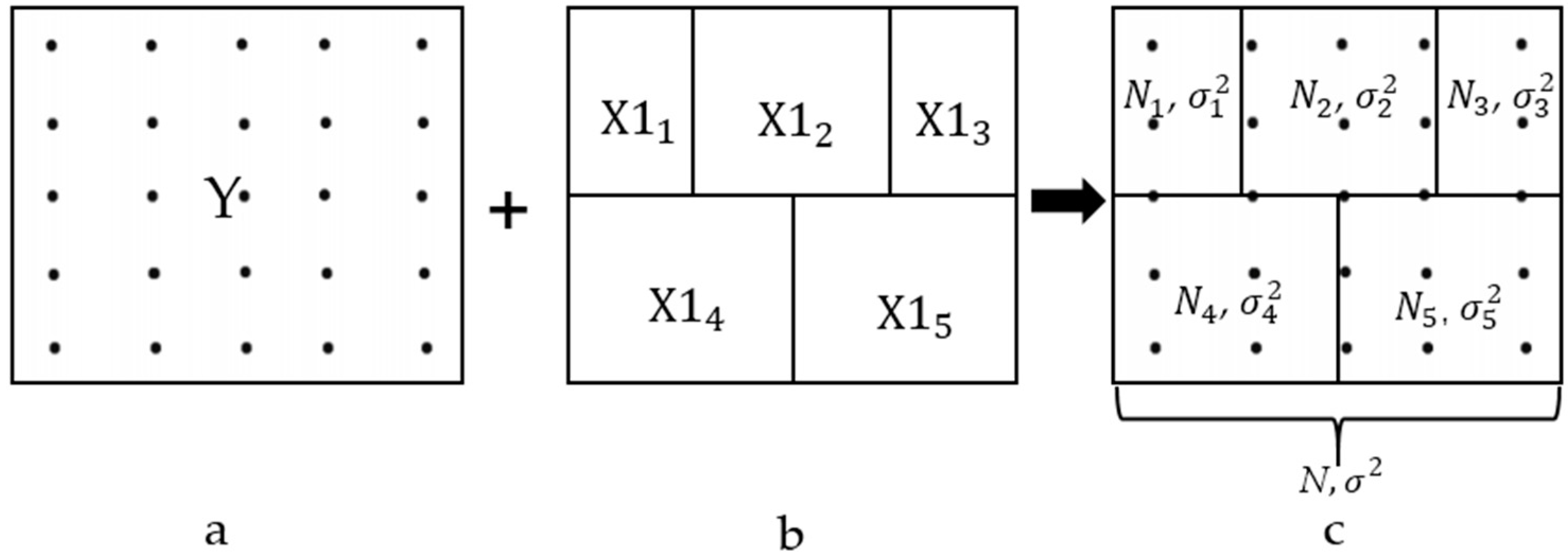
Econometric models are widely used in the study of housing prices to measure the marginal prices of influencing factors. However, with their weakness due to the linear hypothesis, they fail to measure the difference in the magnitude of related factors and their spatial interaction in the complicated spatial relationship of the housing market. As a spatial analysis method, the geographical detector model is constructed based on the simple hypothesis of the linear relationship compared with econometric models. It is used to explore the magnitude of the spatial correlation between the dependent variable and the independent variable by measuring the consistency of variables in spatial distribution. It was first used to detect disease risks [40], and since then has gained increased attention in different fields. For example, using this model, Zhan et al. [41] found that the six dimensions of urban livability more strongly influence urban life satisfaction than the socio-economic attributes of housing type and education level. Liu et al. [42] used geographical detectors to evaluate the spatial inequality of utility-cost value of subway stations between different areas in Chongqing. By probing into county-level housing prices in the Chinese market, Wang et al. [43] found that land cost has a greater impact on housing prices than wages, floating population, and urban service quality.

Notably, the externality of public service resources does not only refer to its capitalization effect on the housing market, but also to its further influence on urban social space through the screening mechanism of housing prices. Research based on Shanghai, China, shows the value of housing and the accessibility to public service facilities are highly spatially consistent. The wealthy live in high-priced communities with higher public service accessibility in the central city, while the poor have to move away from the centre to the outer suburban areas [44]. An investigation into Nanjing, China, also revealed that middle classes agglomerate in school areas due to an unbalanced supply of excellent education resources, which means in the high-priced districts with key middle and higher schools, well-educated white-collar workers comprise 80% of the residents [45]. In other words, the interaction between the supply of local public resources and the housing market produces some exclusive communities, which reinforces the spatial inequality dominated by income gap [46,47].

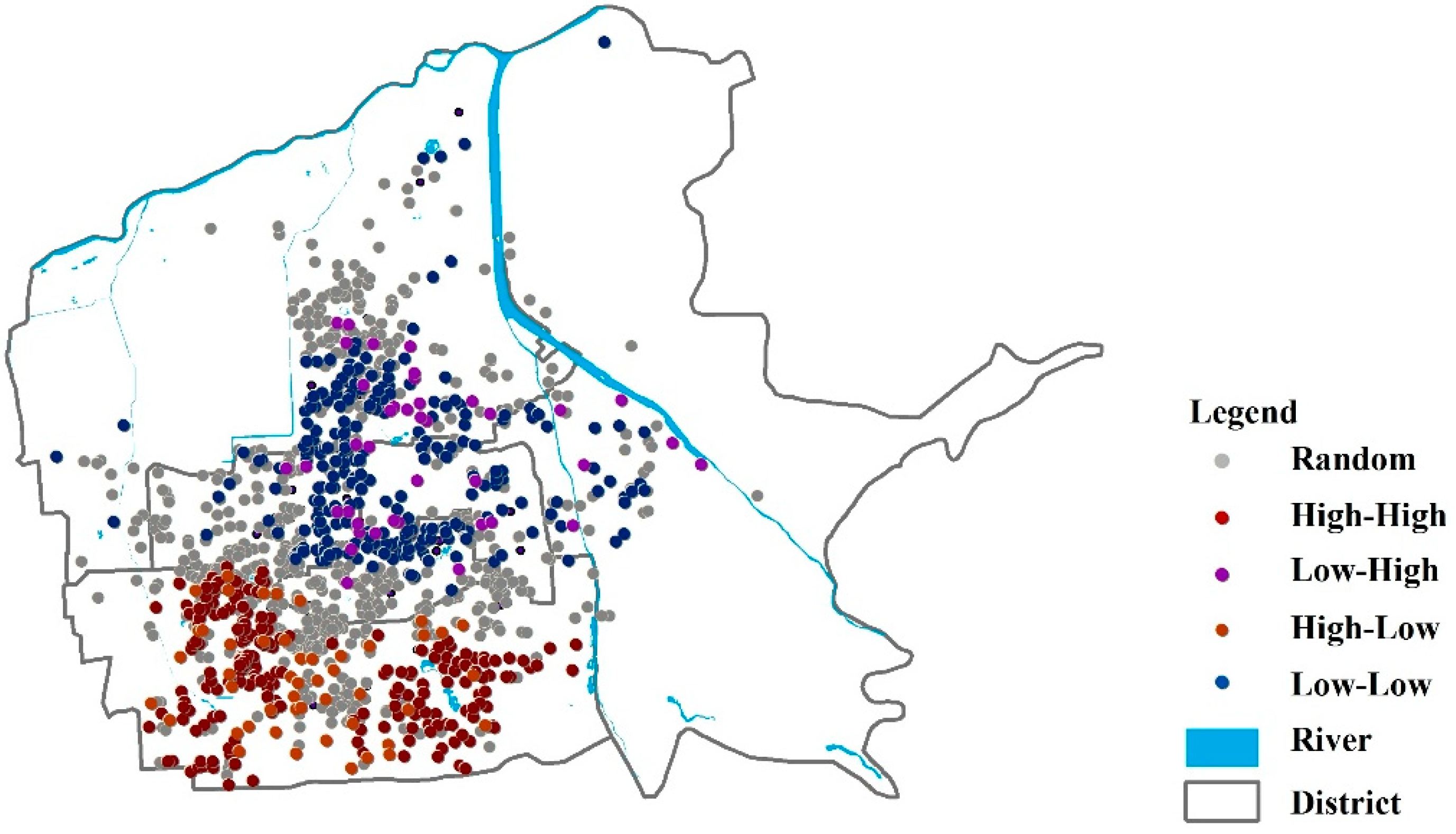
Much of the existing research analysis focuses on the significance and direction of the influence of a certain kind of facility on housing prices by using traditional hedonic price models, spatial error models, geographical weighted regression models, and other econometric models all based on linear hypothesis. Little attention, however, has been paid to the motivation for house price differentiation in terms of urban public service resource allocation. Seldom are the differences in the influence and the multiple spatial interaction effects of different types of public service facilities on housing prices with complex spatial relationships explored. From this perspective, taking Xi’an as an example, we analyzed housing price differentiation using spatial autocorrelation and the access to different public service facilities using a buffer tool of Geographic Information System (GIS). We also explored the direction of the influence of public service facilities on housing prices in different locations with a mixed geographical regression (MGWR) model. We adopted a geographical detector (GD) model to investigate the influence of the accessibility of different urban public service facilities on the distribution of housing prices and the multiple spatial interactions of various facilities.

3. Data and Model

3.1. Study Area and Data Sources

Xi’an, located in Northwest China, is the provincial capital of Shaanxi province. It covers an area of about 3866 km², with a permanent population of about 7.14 million people. Its urban area, covering an area of around 832.17 km², consists of six districts: Xincheng District, Beilin District, Lianhu District, Baqiao District, Weiyang District, and Yanta District. These districts have experienced rapid development as a result of urbanization, thus showcasing the development status and resource allocation of residential space in Xi’an. Accordingly, housing data for the districts were used to explore the impact of public service facilities’ accessibility on housing prices. With housing marketization ongoing, the stock of housing continues to rise and the second-hand housing market has experienced a rising number of transactions. Second-hand housing prices have become an important indicator of the housing market. Compared with the prices of newly-built commercial houses, second-hand housing prices are less controlled by the pricing strategy of developers. Such prices also provide a wider coverage, and can fully reflect the spatial distribution of the housing prices [48]. Notably, residential communities account for 90% of China’s housing market, which are designed and built by single developers [49]. Apartments in the same community share the same location and accessibility. Residents in the same community are alike in their social and economic status. Therefore, to explore house price differentiation associated with public service facilities’ accessibility, the communities in the six main urban districts were defined as the research object and the community-level second-hand housing prices as the dependent variable in this study.

We collected data of second-hand houses across 1253 communities in September 2017 in Xi’an’s six urban districts from Soufun [50] and Anjukelnc [51], both major real estate information source networks with highly credible data. Such enormous sample sizes pose challenges to manual collection of the corresponding online information, but we utilized automatic web crawler technology to facilitate online data collection. The data collected covered the second-hand housing prices of 1253 communities (the average price of all the sold second-hand apartments in the communities in September 2017), floor space ratio (gross floor area to the size of the piece of land for buildings), ratio of green space (the green space to the planned area for construction), management fee, and construction age. The location attributes and neighborhood attributes of the house are related to its location. The position coordinates data, including the latitude and longitude of the house, traditional central business district (CBD) (Bell Tower district), newly emerged CBD (Xiaozhai), and various public service facilities, were obtained from Gaode map [52] using web crawler technology. Based on residents’ demands for public service facilities for work and life, we classified public service facilities into: educational, medical, commercial, leisure, cultural and sports, and financial. Among these, educational facilities refer to top education resources, such as first-class primary schools, best secondary schools, and quality high schools at the provincial level. Medical facilities include general hospitals, specialized hospitals, and community health service stations. Commercial facilities include supermarkets, shopping malls, and local-style commercial streets. Leisure facilities involve city parks, city squares and scenic parks, such as the North Square of the Wild Goose Pagoda and the Tang Paradise. Cultural and sports facilities cover libraries, art galleries, museums, cultural venues, theaters, exhibition centers, and various physical fitness facilities. Financial facilities refer to bank outlets. A detailed description of the data sources is shown in

Table 1. Descriptions of data sources.

Data Source	Description	Information
Soufun Anjukelnc	Soufun and Anjukelnc are databases integrating information on real estate, housing, and price, with the former being China’s largest home networking platform, and the latter being the leading real estate platform for rental and sales service, and related information.	Housing price, floor space ratio (FSR), ratio of green space, management fee, and construction age of second-hand house across 1253 communities in the six main districts of Xi’an in September 2017
Gaode map	Gaode map, developed by Gaode software company, China’s leading provider of digital map, navigation, and location services solutions, offers POI (point of interest) information including name, category, and coordinates.	Location coordinate of facilities regarding education, commerce, leisure, cultural and sports, finance, traditional central business district (CBD) (Bell Tower), and newly emerged CBD (Xiaozhai) in the six main districts of Xi’an in September 2017

Note: The community-level housing price in the above databases refers to the average price of all the sold second-hand apartments in the communities in September 2017.

.

The Standard for Planning and Design on Urban Residential Areas (2018), approved by the Chinese government, specifies the reasonable service radius for public service facilities as a 15-min walking accessibility. Simply put, public service should be provided within the residents’ 15-min walking area. Therefore, we measured the public service facilities’ accessibility based on the number of facilities within a 15-min walking distance. Supposing a walking speed of 4 km/h, a resident will travel 1 km in 15 min [49]. Therefore, the number of facilities within 1 km around a community was used to measure the walking accessibility of public service facilities. The buffer analysis tool in GIS software (ESRI, Redlands, CA, USA) was used for measurement. The distance from communities to the Bell Tower district, the traditional CBD, and the Xiaozhai district—the new CBD (NCBD)—was measured using the near analysis tool in GIS.

Guided by the hedonic price theory, 12 variables covering structural attributes, neighborhood attributes, and location attributes of the housing were regarded as influential factors. The accessibility of the six types of public service facilities was defined as 6 neighborhood characteristic variables to support the focus of this study. The other 6 variables included 4 structural attributes and 2 location attributes, which were selected as control variables. Structural attributes included floor space ratio (FSR), the ratio of green space (GREEN), management fee (FEE), and age of the building (AGE). Neighborhood attributes were the six types of public service facilities within the 1 km buffer radius (EDUCATION, MEDICAL, COMMERCE, LEISURE, C&S, and BANK). The location attributes refer to the distance to the Bell Tower district, the traditional CBD (CBD), and the distance to the NCBD. In order to obtain a clearer distribution of public services’ regression coefficients, which reflect the spatial difference in the relationship between public services and housing price, variables were adopted in linear form. The variable definitions are shown in

Table 2. Variables affecting housing prices and their descriptions.

Attributes Type	Variable	Variable Definition
Structural attributes	FSR	Gross floor area to the size of the piece of land for buildings
	GREEN	Green space to the planned area for construction
	FEE	Property management fees
	AGE	From the year of housing build to 2017
Neighborhood attributes	EDUCATION	Number of schools within 1 km of the community
	MEDICAL	Number of medical facilities within 1 km of the community
	COMMERCE	Number of commercial facilities within 1 km of the community
	LEISURE	Number of leisure facilities within 1 km of the community
	C&S	Number of cultural and sports facilities within 1 km of the community
	BANK	Number of financial facilities within 1 km of the community
Location attributes	CBD	Distance to the CBD (Bell Tower)
	NCBD	Distance to the new CBD (Xiaozhai)

Note: FSR is floor space ratio, GREEN is the ratio of green space, FEE is management fee, AGE is the age of the building, EDUCATION is educational facilities, MEDICAL is medical facilities, COMMERCE is commercial facilities, LEISURE is leisure facilities, C&S is cultural and sports facilities, BANK is financial facilities, CBD is traditional central business district, NCBD is newly central business district.

, and the descriptive statistics of the data are shown in

Table 3. Descriptive statistics.

Variable	Sample Size	Unit	Minimum	Maximum	Mean	SD
PRICE	1253	CNY/m2	3025	26,853	8770	3056.511
FSR	1253	/	0.08	14.1	3.71	1.722
GREEN	1253	/	0.2	0.63	0.36	0.075
FEE	1253	CNY/m2/month	0.2	6	1.21	0.507
AGE	1253	year	0	22	7.65	5.015
EDUCATION	1253	a	0	9	1.59	1.865
MEDICAL	1253	a	0	26	6.21	5.341
COMMERCE	1253	a	0	93	18.71	13.903
LEISURE	1253	a	0	19	2.42	2.821
C&S	1253	a	0	123	29	23.429
BANK	1253	a	0	58	21.81	13.772
CBD	1253	km	0.17	22.31	6.16	2.820
NCBD	1253	km	0.14	26.15	6.95	3.696

Note: SD is standard error. PRICE is housing price.

.

3.2. Model Specification

3.2.1. Mixed Geographically Weighted Regression Model

According to the hedonic price theory, the factors affecting housing prices were divided into structure, neighborhood, and location. Traditional regression models measure the marginal impact of different characteristic factors on housing prices, yet ignore the spatial heterogeneity of housing prices, leading to an estimation bias. The geographical weighted regression model proposed by Fotheringham et al. [53] is an effective local regression model to manage spatial heterogeneity. The regression coefficients of each sample in different locations were computed by the weighted least squares method, which are denoted as follows:

$$Y_i{=\beta }_0\left(u_i{, v}_i\right)+{{\displaystyle \sum }}_{j=1}^q{\beta }_j\left(u_i{, v}_i\right)x_{ij}{+\epsilon }_i, i=1,2,\dots ,n,$$

(1)

where $\left(u_i{, v}_i\right)$ represents the location coordinates of the housing at location i; ${\beta }_0\left(u_i{, v}_i\right)$ and ${\beta }_j\left(u_i{,v}_i\right)$ (j = k + 1, …, q) are the intercept term and the coefficient of local variable j at location i, respectively; $Y_i$ is the house price at location i; $x_{ij}$ is the value of the jth variable at location i; and ${\epsilon }_i$ is the error term at location i.

However, spatial stationarity and spatial non-stationarity may appear simultaneously in the real housing market [38], which limits the application of the model. The model is an integrated result of the traditional linear regression model and the geographical weighted regression model, in which some independent variables are the global variables of the fixed parameters, and the rest are the local variables varying with location. The model avoids the poorly grounded assumption that the spatial relationship between variables is either completely homogeneous or completely heterogeneous. Instead, it more accurately describes the spatial relationship of variables, and is implemented by GWR4.0 software (GWR4.0 development team, Kyoto, Japan). The model is denoted as:

$$Y_i={{\displaystyle \sum }}_{j=1}^k{\alpha }_j{x}_{ij}{+\beta }_0\left(u_i{,v}_i\right)+{{\displaystyle \sum }}_{j=k+1}^q{\beta }_j\left(u_i{,v}_i\right)x_{ij}{+\epsilon }_i, i=1,2,\dots ,n,$$

(2)

where ${\alpha }_j$(j = 1, 2, …, k) are the fixed coefficients of global variables; $\left(u_i{, v}_i\right)$ is the location coordinates of the housing at location i; ${\beta }_0\left(u_i{, v}_i\right)$ and ${\beta }_j\left(u_i{, v}_i\right)$/(j = k + 1, …, q) are the intercept term and the coefficient of local variable j at location i, respectively; $Y_i$ is the house price at location i; $x_{ij}$ is the value of the jth variable at location i; and ${\epsilon }_i$ is the error term at location i. We mainly determined whether the independent variable was global or local through the results of the geographical variability test.

3.2.2. Geographical Detector

Geographical detector is a statistical method for detecting spatial stratified heterogeneity and revealing the driving forces behind a certain phenomenon [54]. It was first applied for the detection of disease risks and has been widely used in the research fields of sociology, public health, and the environment. The factor detector and interaction detector in the geographical detector were used in our study. The factor detector can detect the effect of magnitude of influencing factors (Xn) on housing prices (Y). The interaction detector can reveal whether the influencing factors X1 and X2 have an interactive influence on housing price (Y). Such analyses are performed by the geo-detector software (Chinese Academy of Sciences, Beijing, China). Compared with stereotypical regression models, the model can recognize the magnitude of spatial correlation of two variables without a linear hypothesis; in addition, it can detect the spatial interaction effect not in the form of variable multiplication. In this study, the influencing factors Xn (n = 1, …, 6) are six types of public facilities, and the dependent variable is housing prices. Notably, geo-detector requires that each independent variable comprises categorical data, so we divided the facility accessibility into five levels according to the number of facilities in 1 km buffers in the communities.

The core idea of the factor detector was to test the effect magnitude of accessibility of public services (Xn) on house price (Y) by identifying the degree of consistency of spatial distribution between them. Specifically, the procedure compares the sum of variances of subareas divided by levels of independent variables and the variance of the entire study area. The explanatory power P is defined by Equation (3) and its value varies within [0, 1], so the larger the value of P, the greater the impact of Xn:

$$P=1-\frac{1}{N{\sigma }^2}{{\displaystyle \sum }}_{i=1}^m{N}_i{\sigma }_i^2$$

(3)

where $P$ is the explanatory power of public service facilities (Xn) on house price (Y); m is the classification number of an independent variable, that is, the five levels of accessibility; N and $N_i$ are the numbers of the samples in the whole study area and in sub-region i, which refers to the area with ith level accessibility, respectively; and ${\sigma }^2$ and ${\sigma }_i^2$ are the variances of housing prices of the whole study area and that of sub-region i, which refers to the area with ith level accessibility, respectively.

The principle of the factor detector is shown in Figure 1. Figure 1a,b shows the distribution of house price Y and the variance of facility X1’s five subareas according to accessibility, respectively. As is shown in Figure 1c, to explore the impact of accessibility to facility X1 on house price Y, housing prices should be divided according to the partition shown in Figure 1b. Then, we compared the sum of the variances of the five subareas with the variance of the entire study area, which enabled us to calculate the explanatory power $P_{X1}$.

The above-mentioned factor detector can only explore the influence of a single factor. Yet, different factors may affect each other. The interaction detector can analyze the joint effect of two influencing factors. The interaction principle is shown in Figure 2. It is assumed that X1 and X2 are two types of facilities. Figure 2a is the housing prices pattern. Figure 2b,c are five areas divided by the accessibility of facility X1 and X2, respectively. When they were overlaid, a new partition X1∩X2 (Figure 2d) formed, where ∩ means that the two facilities work together. Based on Equation (3), the influence of X1∩X2 on house price Y is calculated as $P_{X1\cap X2}$.

If P_X1∩PX2 < min(P_X1, P_X2), the interaction shows a nonlinear-weakened effect; if, min(P_X1, P_X2) < P_X1∩PX2 < max(P_X1, P_X2), it shows a uni-weakened effect. If max(P_X1, P_X2) < P_X1∩PX2 < P_X1 + P_X2, it shows a bivariate-enhanced effect; if P_X1∩PX2 > P_X1 + P_X2, it shows a nonlinear-enhanced effect; and, if P_X1∩PX2 = P_X1 + P_X2, factors X1 and X2 are independent.

4. Results

4.1. Spatial Auto-Correlation

Spatial autocorrelation means variables in geographically close locations have similar values. In this paper, the Moran’s I and local indicators of spatial association (LISA) are used to examine the global spatial autocorrelation and local spatial autocorrelation of housing prices, respectively. The Moran’s I index was 0.262, and the statistic value Z was 5.549, indicating a spatial autocorrelation in housing prices in Xi’an, meaning nearby communities have similar housing prices.

The LISA index can identify the local agglomeration of housing prices. The LISA agglomeration was visualized to show the local spatial agglomeration of housing prices (Figure 3). “High-High” refers to a high-priced cluster, indicating that high-priced communities are surrounded by similar communities. Similarly, “Low-Low” refers to a low-priced cluster. “High-Low” and “Low-High” refer to communities surrounded by those with significantly different prices. There were distinct high-priced clusters and low-priced clusters of housing prices in Xi’an. The high-value clusters were in the newly-developed Qujiang District and high-tech zone in the south urban area of Xi’an. The low-value clusters existed in the inner city and the nearby northeastern area, and there were several low-value points located in the urban fringe areas such as Sanqiao Street in the west of the city and Xujiawan Street in the north of the city.

4.2. Pattern of Accessibility of Public Services

Based on the buffer analysis of GIS software, the accessibility of the six types of public service facilities was depicted using the fishing net tools in GIS (Figure 4). In general, the accessibility of the public service resources in Xi’an showed a center–periphery pattern. It was significantly clustered in the core urban areas (Lianhu District, Xincheng District, and Beilin District), especially in the area within the city wall. The high-quality education resources—for example, the Middle School attached to Northwestern Polytechnical, the famous commercial streets (such as East and West Streets, and North and South Streets), and the Forest of Stelae Museum—are all within the area, promoting the comprehensive development of the old urban areas. In contrast, there was a larger gap between the accessibility of public service facilities in urban fringe areas and that in core urban areas.

We observed different cluster distributions of these facilities due to the functional differences in each area of the city. High-quality schools, like Xi’an Gaoxin No. 1 Primary School, are located in a high-tech zone. Cultural and sports facilities, such as the Provincial History Museum, are concentrated in the south of the city. A cluster of high-end shopping malls was found in Xiaozhai, a new CBD of Xi’an. Another high-accessibility cluster of cultural and leisure facilities, such as the North Square of Great Wild Goose Pagoda and the Tang Paradise, are located in the newly developed Qujiang District in the southeast of the city. The Economic Development Zone, as an emerging development zone, has attracted many financial resources.

4.3. Results of the Mixed Geographically Weighted Regression (MGWR) Model

With GWR4.0 software, the geographical variability tests were conducted using 12 characteristic variables in the geographically weighted regression model, and the results are shown in

Table 4. The results of the geographical variability test of the geographically weighted regression (GWR) model.

Variable	Difference in Criterion
PLOT	−48.99
GREEN	18.94
FEE	−41.78
AGE	−19.94
EDUCATION	−3.50
MEDICAL	−3.50
COMMERCE	11.37
LEISURE	9.06
C&S	−0.58
BANK	−2.51
CBD	4.74
NCBD	−18.78

Note: Variables with negative values of Difference in criterion indicate spatial non-stationarity.

. These four factors (GREEN, COMMERCE, LEISURE, and CBD), failing to pass the spatial instability test, were considered as global variables in the MGWR model. The remainder were local variables. The kernel type was adaptive bi-square, and the optimal bandwidth of the MGWR model was calculated according to the Akaike information criterion (AIC).

Table 5. Comparison of fitting results between global ordinary least squares (OLS) regression, geographically weighted regression (GWR), and mixed geographically weighted regression (MGWR) models.

Model Parameter	OLS	GWR	MGWR
Akaike information criterion (AICC)	22,963.370	22,661.247	22,611.501
R2	0.443	0.669	0.673
Adjusted R2	0.437	0.601	0.613

exhibits the results of the comparison between the global ordinary least squares (OLS), GWR, and MGWR models. Considering the spatial non-stability, the GWR and MGWR models were superior to the OLS model. The MGWR model, which contained global variables and exactly analyzed the influence of factors on housing prices, outperformed the GWR model.

Table 6. The results of global coefficients of MGWR model.

Variable	Coefficient	SD	t-Value
GREEN	333.88 ***	63.325	5.27
COMMERCE	73.42	149.846	0.49
LEISURE	−121.35	98.493	−1.23
CBD	−605.24	451.019	−1.34

Note: *** represents the 1% significance level.

exhibits the regression result of the global variables of the MGWR model. The ratio of green space, commercial facilities, leisure facilities, and the distance from the CBD was spatially stationary. The ratio of green space had a significant positive influence on housing prices.

Table 7. The results of local coefficients of the MGWR model.

Variable	Minimum	Lower Quartile	Median	Upper Quartile	Maximum	Mean	Difference of Criterion
PLOT	−3015.97	−668.40	−191.17	65.16	525.04	−385.86	−121.72
FEE	−376.96	487.12	830.93	1354.21	2603.39	870.63	−107.50
AGE	−2331.53	−1053.20	−637.14	−357.20	61.94	−744.32	−68.32
EDUCATION	−2242.74	−251.86	−26.52	242.28	1477.37	11.74	−0.66
MEDICAL	−3886.86	−774.87	−322.25	74.78	802.22	−500.47	−274.43
C&S	−3090.53	−42.54	309.60	757.59	3732.06	357.78	−63.08
BANK	−2049.31	−382.80	122.09	694.08	3688.59	272.69	−7.83
NCBD	−5064.43	−1501.39	−86.19	1198.13	8712.97	14.22	−10.17

shows a statistical description of the regression coefficients of the local variables. First, according to the results of the geographical variability test, each variable in the “Difference of criterion” column is negative. This finding means that they all showed significant spatial instability; that is, the impact on housing prices varies with locations. Secondly, by comparing the regression coefficients of different variables, all showed a distinct difference in direction. Notably, the signs of the median and the average of the coefficients were much alike in most variables, which demonstrates that these factors had a consistent effect on most housing samples in the region.

This paper focuses on the impact of the accessibility of six types of public service facilities on housing prices, and explores the spatial rule of the groups of public service facilities on housing prices. According to the results of the spatial stationarity test, commercial and leisure facilities were spatially stable, and the global regression results based on linear hypothesis (Table 5) show that the linear relationship between commercial facilities and cultural and sports facilities and housing prices is not remarkable. In comparison, educational, medical, cultural and sports, and financial facilities were spatially non-stationary. Figure 5, Figure 6, Figure 7 and Figure 8 depict local regression coefficients and t values for these four types of facilities. Critical t values of 1.645, 1.960, and 2.576, the upper limit corresponding to 90%, 95%, and 99% confidence levels in the t-test, respectively, were used as the breakpoints to show the distribution of t values. We found that the significance of the public service facilities impacting housing prices is non-stationary when their locations change.

4.3.1. Influence of Educational Facilities

As shown in Figure 5, the accessibility to key schools significantly positively impacted housing prices in most districts. The maximum impact was found in the high-tech zone and newly-developed Qujiang District in the south. With the development of the city, these two districts have become superior areas for residents to live. For example, the high-tech zone, where high-quality schools, such as Xi’an Gaoxin No. 1 High School and Xi’an Gaoxin No. 1 Primary School, are located, is highly regarded by residents for its educational environment, resulting in a dramatic increase in housing prices. In addition, in emerging residential areas, such as the Chan-ba area in the east, the mismatch between the growing demand for housing and an insufficient supply of educational resources makes housing prices more susceptible to the location of key schools.

4.3.2. Influence of Medical Facilities

As shown in Figure 6b, hospital accessibility was significantly correlated in all regions except some in the downtown area. The largest negative impact was found in the well-built residential areas in the south, such as the newly developed Qujiang District and the high-tech zone (Figure 6a). This mainly occurred because problems, such as traffic congestion and environmental pollution, become increasingly severe due to the presence of hospitals, further worsening the living quality of residents. However, a positive impact was found in the urban fringe areas where such facilities are highly sought after due to their shortage.

4.3.3. Influence of Cultural and Sports Facilities

As shown in Figure 7, the influence of cultural and sports facilities on housing prices appears to change gradually from negative to positive from the interior to the exterior, but a less significant correlation was found in the three core urban regions of Beilin, Xincheng, and Lianhu. This is because the facilities are clustered in the three core urban areas and there is a substitution effect between such facilities, so that the housing in this area is less dependent on the facilities. As the city sprawls outward, fewer cultural and sports facilities are found in clusters. Their positive impact on housing prices tends to be pronounced in mature residential areas, such as the newly developed Qujiang District and high-tech zone, and other urban fringe areas, such as Chan-ba.

4.3.4. Influence of Financial Facilities

As shown in Figure 8b, the impact of financial facilities was not significant in most regions, because people are less dependent on financial facilities due to the popularity of electronic-payments. In contrast, a significant impact was found in the west side of the city (Figure 8a). These areas include the high-tech zone in the southwest of the city, where high-end industries are gathered, leading to considerable demand for financial facilities and an acute premium effect.

4.4. Results of the Geographical Detector (GD) Model

4.4.1. Factor Detector

Table 8. The results of factor detector.

Variable	MEDICAL	EDUCATION	COMMERCE	LEISURE	C&S	FINANCIAL
q-statistic	0.0811 ***	0.0457 ***	0.0315 ***	0.0254 **	0.0148 **	0.0088 **

Note: *** and ** represent the 1% and 5% significance levels, respectively.

shows the impacts of different facilities on housing prices based on the factor detector. The results show that the six types of facilities all affected housing price differentiation. Their influence is ranked as follows: medical facilities (8.11%) > educational facilities (4.57%) > commercial facilities (3.15%) > leisure facilities (2.54%) > cultural and sports facilities (1.48%) > financial facilities (0.88%). Among them, commercial facilities and leisure facilities, which were not significant in the MGWR model, were significant in the geographical detector model. This evidences the non-linear spatial associations between commercial and leisure facilities and housing prices.

4.4.2. Interaction Detector

The interaction detector was used to detect the influence of two different factors on housing prices when taken together.

Table 9. The results of interaction detector.

Variable	MEDICAL	EDUCATION	COMMERCE	LEISURE	C&S	FINANCIAL
MEDICAL
EDUCATION	0.0937↑
COMMERCE	0.0979↑	0.0653↑
LEISURE	0.1787↗	0.1690↗	0.1208↗
C&S	0.2050↗	0.1081↗	0.1211↗	0.0585↗
FINANCIAL	0.1531↗	0.0801↗	0.0793↗	0.1053↗	0.0568↗

Note: ↑ represents the bivariate-enhanced effect when max(P_X1, P_X2) < P_X1∩X2 < P_X1 + P_X2, ↗ represents the nonlinear-enhanced effect when P_X1∩X2 > P_X1 + P_X2.

shows the explanatory power of facilities on housing prices due to the interaction between any two of six facilities. By comparing the interaction detection results in Table 9 with those of separate influence in Table 8, we further analyzed the type of interactions (bivariate-enhanced or nonlinear-enhanced). The results showed that medical, educational, and commercial facilities intensify their influence on housing differentiation when interacting with each other. A bivariate-enhanced effect was presented: the interactive influences between educational and medical facilities, educational and commercial facilities, and medical and commercial facilities were greater than the maximum of their separate influences. Notably, although the separate influence of leisure, cultural and sports, and financial facilities on housing prices was relatively weak, an effect of nonlinear enhancement emerged when they interacted with other facilities, indicating the effect of their interaction with others was greater than the sum of their separate influences.

5. Discussion

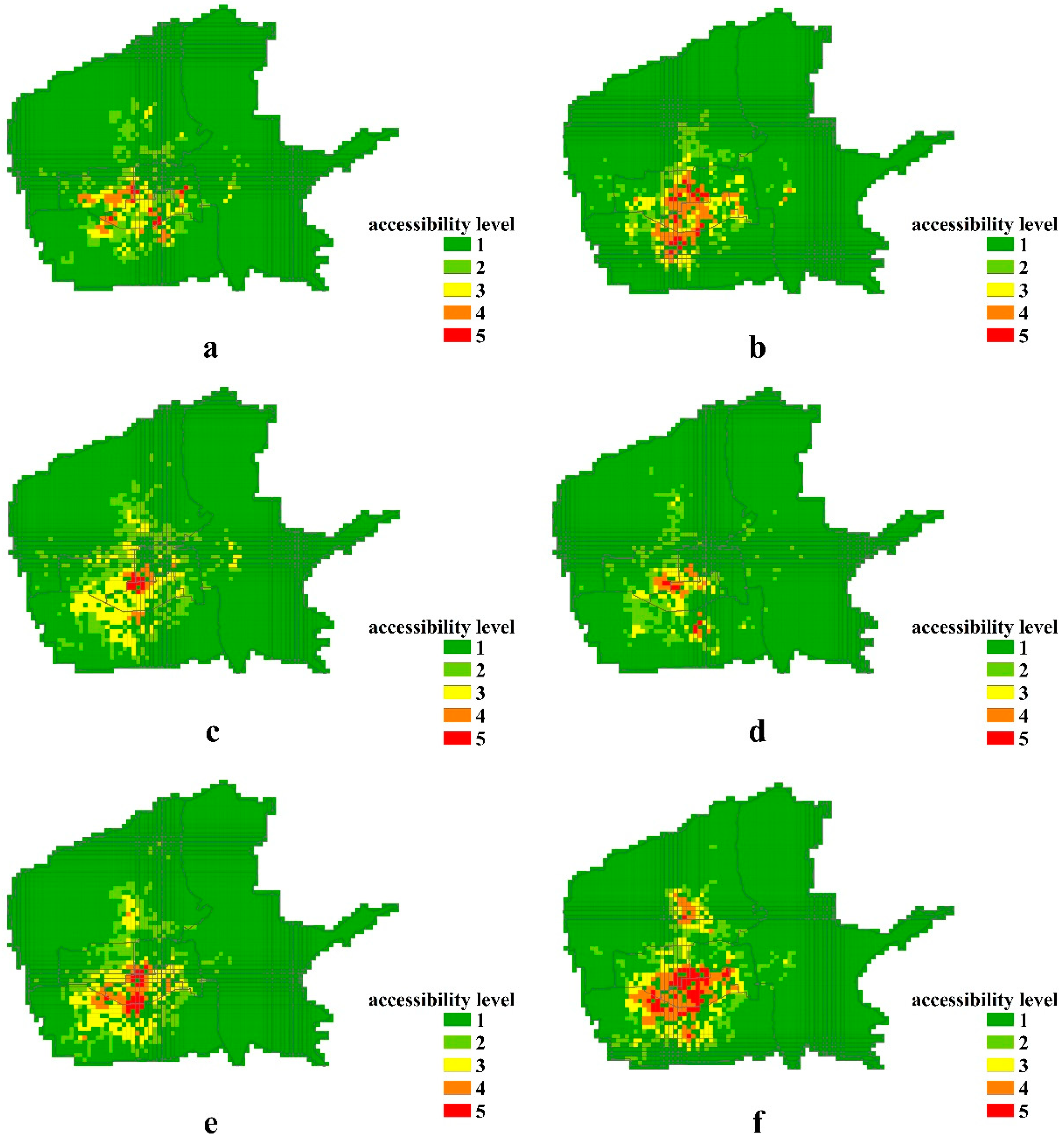
Based on the analysis of housing prices and public service facilities’ accessibility, we found differentiation in both the housing prices and the public service facilities’ accessibility across the city. All types of public service facilities maintained the same pattern of the planned economy period, showing a center–periphery distribution. This pattern also exists in other Chinese cities such as Shanghai and Beijing. Unlike the high-priced cluster in the central areas of these two cities, the downtown area of Xi’an is a surprisingly low-priced cluster. This is explained by the city’s urban master plan, which highlights urban conservation. Protecting heritage sites and the overall spatial pattern of the area around the Ming city wall largely hamper the renewal of Xi’an’s inner city, where decayed communities with poor property management are concentrated. As the city sprawls, clusters of housing prices and disparity of public service have appeared. For example, the high-tech zone has evolved into a new cluster of educational and medical resources. The newly developed Qujiang District, well-known for its rich tourism and cultural resources from the North Square of Wild Goose Pagoda to the Tang Paradise, has been an ideal place for well-to-do families to live. Residents in high-priced communities located in these areas can enjoy quality public service here. In contrast, low-priced communities cluster along urban fringes with low accessibility to public service facilities, where low-income groups are forced to settle. Such marginalization of low-income groups has been a common phenomenon in many cities.

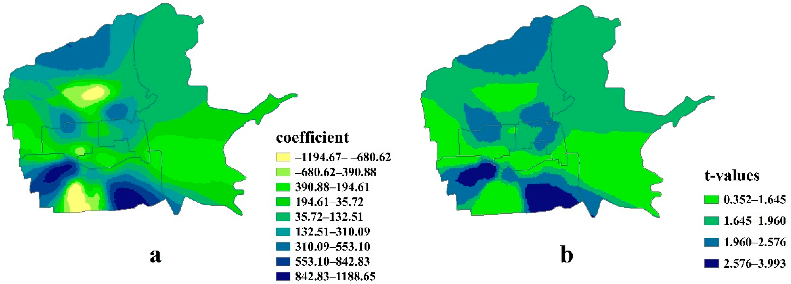
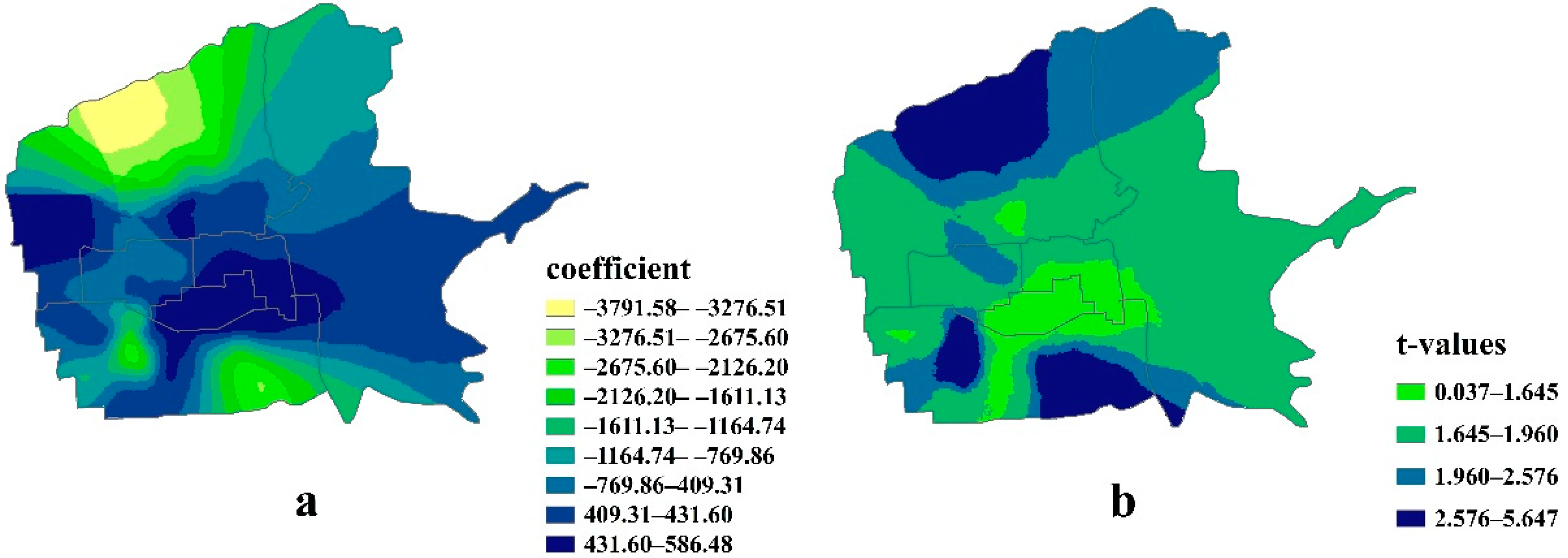
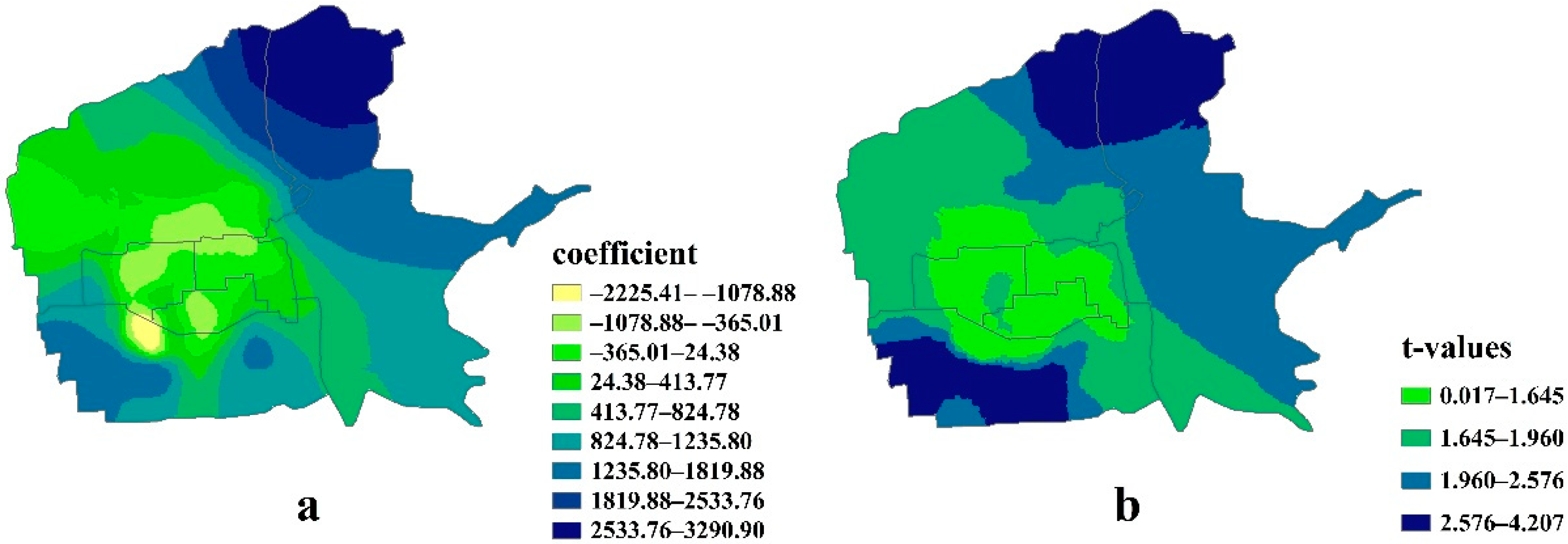
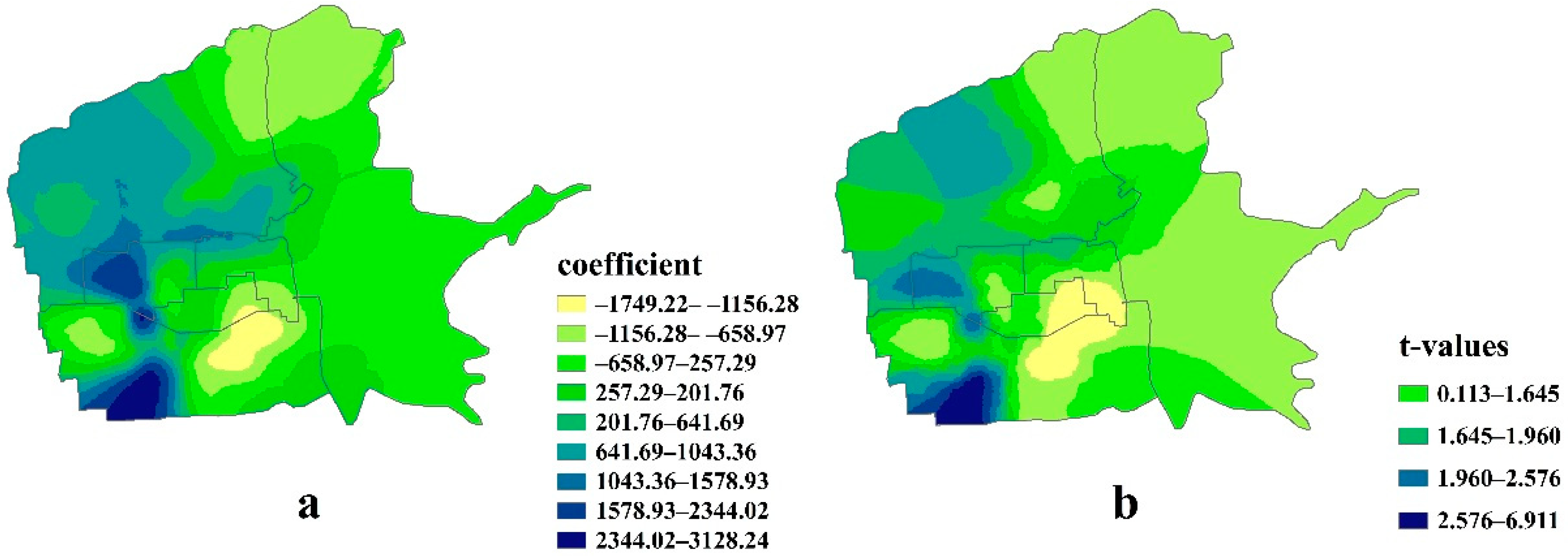
The MGWR model was employed to further explore the spatial impact of accessibility of public service facilities on housing prices. We found that education, medical care, and cultural and sports facilities significantly impacted housing prices, which corresponds to previous studies. For example, Feng et al. [16] noted that a positive relationship exists between housing prices and the number of key secondary schools in each square kilometer. Wu et al. [28] found that urban parks have a 32.23% premium effect on surrounding housing prices in Shenzhen, China. However, these studies assumed that the regression coefficients are fixed in the study area, ignoring the heterogeneity of spatial relationships. We used the MGWR model to explore in-depth associations between housing prices and public service resources. Implicit prices of educational, medical, cultural and sports, and financial facilities varied significantly over space, whereas the impacts of the two remaining facilities on housing prices were fixed throughout the entire study area, which indicates that the MGWR model, handling both spatial stationary and non-stationary effects, produced results that are closer to reality.

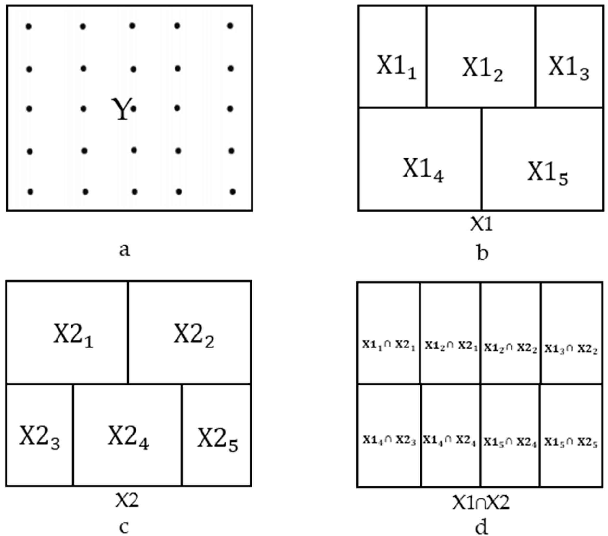
In addition, we used the GD model to explore the magnitude of the influence of accessibility of different urban public service facilities on the distribution of housing prices and the multiple spatial interactions of various facilities. This attempt has rarely been applied in previous studies. An intriguing finding is that the influence of different facilities on housing price differentiation is hierarchical, a result of the demands from residents being hierarchical. Facilities that meet the basic needs of residents, such as medical and educational facilities, play a basic role in house price differentiation. Since ancient times, Chinese families have attached great importance to their children’s education [45], so the quality of educational facilities, a major factor in residential location selection, has a significant effect on increasing surrounding housing prices. The leisure, cultural and sports, and other facilities improve the living quality of residents and meet their higher-level needs when their basic needs have been satisfied. These factors are not necessities for the majority of residents; therefore, the impact of these facilities on house price differentiation is relatively weak.

According to the interaction detector results, the interaction between the facilities meeting the basic needs of people produced a bivariate-enhanced effect. Notably, the interaction between resources for high-level demands and others exerted nonlinear-enhanced effects, revealing that such resources for high-level demands are the interactive elements of the spatial differentiation of housing prices and considerably enhance other resources. The result proves the importance of the interaction between resources for higher-level demands and those for lower demands on house price differentiation. Access to facilities, such as schools and shopping malls, fails to meet the growing needs of residents for a better life. Thus, residents not only focus on these facilities, but also pursue facilities providing higher-level needs, such as parks, theaters, and gyms.

Previous studies have shown that affordability and residents’ social status determine where they live. Housing prices filter different people and drive them to affordable places [55]. The trend not only affects the fair supply of urban resources, but also deepens the residential divide between high-income and low-income people, which is also detrimental to the sustainable development of social space. Accordingly, our study, relating to the capitalization effect of public service facilities on housing prices, provides a reference for the government to formulate housing policies to ensure the housing needs of low-income people are met, and to promote the sustainable development of urban social space.

Although this study draws fruitful conclusions, there is still room for improvement in future research. First, geo-detectors were employed to explore the multiple interaction effects of different facilities, but they were applied to the interaction of two types of factors, and failed in more than two factors. Second, in addition to the impact of the surrounding public service facilities, housing prices are also affected by socio-economic factors such as household income and educational attainment [2,7]. This study concentrated on the spatial differentiation of housing prices from the perspective of spatial allocation of urban public service facilities, without considering the impact of other socio-economic factors, heterogeneous residential demands, or preferences among individuals. Therefore, our future research will focus on different families’ willingness to pay for specific public service facilities based on household survey data, including family structure and household income.

6. Conclusions

Taking Xi’an, China as a case study, we used GIS to describe the spatial distribution of housing prices and urban public service facilities. We also employed a MGWR and a GD to reveal the effects of accessibility of urban public service facilities on house price differentiation. The main conclusions are as follows:

(1)

Distinctive spatial differentiation was found both in housing prices and public service facilities’ accessibility. High-priced clusters were found in the well-built residential areas with higher public service accessibility, whereas low-priced clusters were found in the urban fringes with lower accessibility.

(2)

The commercial and leisure facilities are spatially stationary. The influence of educational, medical, culture and sports, and financial facilities on housing prices varied distinctly with location. The maximum effect of these facilities was identified in urban fringe areas and some well-built residential areas, such as the newly developed Qujiang District and the high-tech zone.

(3)

Housing prices are affected by medical facilities, educational facilities, commercial facilities, leisure facilities, culture and sports facilities, and financial facilities, which are shown in order according to the strength of their impacts. The top three public service facilities are the basic elements influencing house price differentiation. The impact of different facilities on housing prices demonstrated a barrel effect. The synergy from the interaction of different facilities affect house price distribution. Moreover, facilities for high-level needs, such as parks, gyms, and theaters, are key interactive elements of price differentiation.

Housing prices have a potential screening effect on buyers. It is of significant practical value to ensure better spatial patterns of public service facilities, less urban spatial inequality, and more sustainable development of social space by exploring the differentiation in urban housing prices in relation to spatial allocation of public service facilities. The study provides insights for policy-making. First, considering the different effects of various public service resources, which are related to residents’ demands, governments can take a first step by optimizing the allocation of facilities for basic needs, such as schools and hospitals. We also suggest increasing the supply of educational and medical facilities in urban fringe areas, which are characterized by increasing demand and scarce supply. Developers are encouraged to introduce quality schools and medical resources through cooperative partnerships with schools or hospitals, laying a solid foundation for the continuous spatial expansion of the population. Second, in order to protect the basic needs of low-income people, promote residents’ integration, and maintain the sustainable development of social space, governments should implement different indicators of affordable housing construction for developers in different locations. For example, developers should be required to build houses with a higher proportion of affordable housing in urban prime areas with high-quality public service facilities rather than in areas that are poorly facilitated.

This study not only contributes to the research on human living spaces, such as that on the satisfaction of living space, but also extends the application of the GD model from physical geography to urban social development. New insights are thus proposed in exploring the mechanisms driving economic growth imbalances, in particular, the aging population and the spatial interaction effects of decisive factors.

References

1. Ardeshiri, A.; Willis, K.; Ardeshiri, M. Exploring preference homogeneity and heterogeneity for proximity to urban public services. Cities 2018, 81, 190–202. [Google Scholar] [CrossRef]
2. Wu, W.; Zhang, W.; Dong, G. Determinant of residential location choice in a transitional housing market: Evidence based on micro survey from Beijing. Habitat Int. 2013, 39, 16–24. [Google Scholar] [CrossRef]
3. La, V. Capitalization of school quality into the housing prices: Evidence from Boston public school district walk zones. Econ. Lett. 2015, 134, 102–106. [Google Scholar] [CrossRef]
4. Saphores, J.D.; Li, W. Estimating the value of urban green areas: A hedonic pricing analysis of the single-family housing market in Los Angeles, CA. Landsc. Urban Plan. 2012, 104, 373–387. [Google Scholar] [CrossRef]
5. Fack, G.; Grenet, J. When do better schools raise the housing prices? Evidence from Paris public and private schools. J. Public Econ. 2011, 94, 59–77. [Google Scholar] [CrossRef]
6. Jin, P.; Dong, L.; Chan, P.; Kim, H.; Jung, T.; Kim, S. Park accessibility impacts the housing prices in Seoul. Sustainbility 2017, 9, 185. [Google Scholar] [CrossRef]
7. Huang, Z.; Chen, R.; Xu, D.; Zhou, W. Spatial and hedonic analysis of the housing prices in Shanghai. Habitat Int. 2017, 67, 69–78. [Google Scholar] [CrossRef]
8. Song, W.; Liu, C. Spatial differentiation of gated communities in Nanjing. Int. J. Urban Sci. 2017, 21, 312–325. [Google Scholar] [CrossRef]
9. Song, W.; Mao, N.; Chen, P.; Yuan, Y.; Wang, Y. Coupling mechanism and spatial-temporal pattern of residential differentiation from the perspective of the housing prices: A case study of Nanjing. Acta Geogr. Sin. 2017, 72, 589–602. (In Chinese) [Google Scholar]
10. Xu, Y.; Song, W.; Liu, C. Social-Spatial accessibility to urban educational resources under the school district system: A Case Study of Public Primary Schools in Nanjing, China. Sustainability 2018, 10, 2305. [Google Scholar] [CrossRef]
11. Wen, H.; Xiao, Y.; Zhang, L. Spatial effect of river landscape on housing price: An empirical study on the Grand Canal in Hangzhou, China. Habitat Int. 2017, 63, 34–44. [Google Scholar] [CrossRef]
12. Wen, H.; Gui, Z.; Tian, C.; Xiao, Y.; Fang, L. Subway Opening, Traffic Accessibility, and the housing prices: A Quantile Hedonic Analysis in Hangzhou, China. Sustainability 2018, 10, 2254. [Google Scholar] [CrossRef]
13. Dai, X.; Bai, X.; Xu, M. The influence of Beijing rail transfer stations on surrounding the housing price. Habitat Int. 2016, 55, 79–88. [Google Scholar] [CrossRef]
14. Wen, H.; Xiao, Y.; Zhang, L. School district, education quality, and housing price: Evidence from a natural experiment in Hangzhou, China. Cities 2017, 66, 72–80. [Google Scholar] [CrossRef]
15. Hui, E.C.; Liang, C. Spatial spillover effect of urban landscape views on property price. Appl. Geogr. 2016, 72, 26–35. [Google Scholar] [CrossRef]
16. Feng, H.; Lu, M. School quality and the housing prices: Empirical evidence from a natural experiment in Shanghai, China. J. Hous. Econ. 2013, 22, 291–307. [Google Scholar] [CrossRef]
17. Jim, C.Y.; Chen, W.Y. External effects of neighborhood parks and landscape elements on high-rise residential value. Land Use Policy 2010, 27, 662–670. [Google Scholar] [CrossRef]
18. Chiang, Y.H.; Peng, T.C.; Chang, C.O. The nonlinear effect of convenience stores on residential property prices: A case study of Taipei, Taiwan. Habitat Int. 2015, 46, 82–90. [Google Scholar] [CrossRef]
19. Kuang, C. Does quality matter in local consumption amenities? An empirical investigation with yelp. J. Urban Econ. 2018, 100, 1–18. [Google Scholar] [CrossRef]
20. Bae, H.; Chung, I.H. Impact of school quality on house prices and estimation of parental demand for good schools in Korea. Kedi J. Educ. Policy 2013, 10, 43–61. [Google Scholar]
21. Gibbons, S.; Mourato, S.; Resende, G.M. The amenity value of English nature: A hedonic price approach. Environ. Resour. Econ. 2014, 57, 175–196. [Google Scholar] [CrossRef] [Green Version]
22. Lin, I.H.; Wu, C.; Sousa, C.D. Examining the economic impact of park facilities on neigh-boring residential property values. Appl. Geogr. 2013, 45, 322–331. [Google Scholar] [CrossRef]
23. Melichar, J. Revealing preferences of Prague’s homebuyers toward greenery amenities: The empirical evidence of distance–size effect. Landsc. Urban Plan. 2013, 109, 56–66. [Google Scholar] [CrossRef]
24. Jayantha, W.M.; Lam, S.O. Capitalization of secondary school education into property values: A case study in Hong Kong. Habitat Int. 2015, 50, 12–22. [Google Scholar] [CrossRef]
25. Andreyeva, E.; Patrick, C. Paying for priority in school choice: Capitalization effects of charter school admission zones. J. Urban Econ. 2017, 100, 19–32. [Google Scholar] [CrossRef]
26. Hu, W.; Zheng, S.; Wang, R. The capitalization of school quality in home value: A matching regression approach with housing price-rent comparison. China Econ. Q. 2014, 13, 1195–1214. (In Chinese) [Google Scholar]
27. Jung, E.; Choi, Y.; Yoon, H. The impact of the Gyeongui Line Park project on residential property values in Seoul, Korea. Habitat Int. 2016, 58, 108–117. [Google Scholar] [CrossRef]
28. Wu, C.; Ye, X.; Du, Q.; Luo, P. Spatial effects of accessibility to parks on the housing price in Shenzhen, China. Habitat Int. 2017, 63, 45–54. [Google Scholar] [CrossRef]
29. Panduro, T.E.; Veie, K.L. Classification and valuation of urban green spaces—A hedonic house price valuation. Landsc. Urban Plan. 2013, 120, 119–128. [Google Scholar] [CrossRef]
30. Jun, M.J.; Kim, H.J. Measuring the effect of greenbelt proximity on apartment rents in Seoul. Cities 2017, 62, 10–22. [Google Scholar] [CrossRef]
31. Feng, X.; Humphreys, B.R. The impact of professional sports facilities on housing values: Evidence from census block group data. City Cult. Soc. 2012, 3, 189–200. [Google Scholar] [CrossRef]
32. Small, K.A.; Steimetz, S.S. Spatial hedonics and the willingness to pay for residential amenities. J. Reg. Sci. 2012, 52, 635–647. [Google Scholar] [CrossRef]
33. Hanink, D.M.; Cromley, R.G.; Ebenstein, A.Y. Spatial variation in the determinants of house prices and apartment rents in China. J. Real Estate Finance Econ. 2012, 45, 347–363. [Google Scholar] [CrossRef]
34. Nilsson, P. Natural amenities in urban space—A geographically weighted regression approach. Landsc. Urban Plan. 2014, 121, 45–54. [Google Scholar] [CrossRef]
35. Li, H.; Wei, Y.D.; Yu, Z.; Tian, G. Amenity, accessibility and housing values in metropolitan USA: A study of Salt Lake County, Utah. Cities 2016, 59, 113–125. [Google Scholar] [CrossRef]
36. McCord, M.; Davis, P.T.; Haran, M.; McGreal, S.; McIlhatton, D. Spatial variation as a determinant of house price: Incorporating a geographically weighted regression approach within the Belfast housing market. J. Financ. Manag. Prop. Constr. 2012, 17, 49–72. [Google Scholar] [CrossRef]
37. Crespo, R.; Grêt-Regamey, A. Local hedonic house-price modelling for urban planners: Advantages of using local regression techniques. Environ. Plan. B Plan. Des. 2013, 40, 664–682. [Google Scholar] [CrossRef]
38. Helbich, M.; Brunauer, W.; Vaz, E.; Nijkamp, P. Spatial heterogeneity in hedonic house price models: The case of Austria. Urban Stud. 2014, 51, 390–411. [Google Scholar] [CrossRef]
39. Wen, H.; Jin, Y.; Zhang, L. Spatial heterogeneity in implicit the housing price: Evidence from Hangzhou, China. Int. J. Strat. Prop. Manag. 2017, 21, 15–28. [Google Scholar] [CrossRef]
40. Wang, J.; Li, X.; Christakos, G.; Liao, Y.; Zhang, T.; Gu, X.; Zheng, X. Geographical detectors-based health risk assessment and its application in the neural tube defects study of the Heshun Region, China. Int. J. Geogr. Inf. Sci. 2010, 24, 107–127. [Google Scholar] [CrossRef]
41. Zhan, D.; Kwan, M.P.; Zhang, W.; Fan, J.; Yu, J.; Dang, Y. Assessment and determinants of satisfaction with urban livability in China. Cities 2018, 79, 92–101. [Google Scholar] [CrossRef]
42. Liu, X.; Macedo, J.; Zhou, T.; Shen, L.; Liao, Y.; Zhou, Y. Evaluation of the utility efficiency of subway stations based on spatial information from public social media. Habitat Int. 2018, 79, 10–17. [Google Scholar] [CrossRef]
43. Wang, Y.; Wang, S.; Li, G.; Zhang, H.; Jin, L.; Su, Y.; Wu, K. Identifying the determinants of the housing price in China using spatial regression and the geographical detector technique. Appl. Geogr. 2017, 79, 26–36. [Google Scholar] [CrossRef]
44. Li, H.; Wang, Q.; Shi, W.; Deng, Z.; Wang, H. Residential clustering and spatial access to public services in Shanghai. Habitat Int. 2015, 46, 119–129. [Google Scholar] [CrossRef]
45. Wu, Q.; Zhang, X.; Waley, P. Jiaoyufication: When gentrification goes to school in the Chinese inner city. Urban Stud. 2016, 53, 3510–3526. [Google Scholar] [CrossRef] [Green Version]
46. Sun, W.; Fu, Y.; Zheng, S. Local Public Service Provision and Spatial Inequality in Chinese Cities: The Role of Residential Income Sorting and Land-Use Conditions. J. Reg. Sci. 2017, 57, 547–567. [Google Scholar] [CrossRef]
47. Owens, A. Inequality in children’s contexts: Income segregation of households with and without children. Am. Sociol. Rev. 2016, 81, 549–574. [Google Scholar] [CrossRef]
48. Wang, F.; Gao, Q.; Yan, B. Research on urban spatial structure in Beijing based on the housing price. Prog. Geogr. 2014, 33, 1322–1331. (In Chinese) [Google Scholar]
49. Wen, H.; Xiao, Y.; Hui, E.C.; Zhang, L. Education quality, accessibility, and housing price: Does spatial heterogeneity exist in education capitalization? Habitat Int. 2018, 78, 68–82. [Google Scholar] [CrossRef]
50. Soufun Real Estate Trading Platform. Housing Price, Floor Space Ratio (FSR), Ratio of Green Space, Management Fee, and Construction Age of Communities. Available online: http://xian.fang.com/ (accessed on 28 September 2017).
51. Anjukelnc Real Estate Trading Platform. Housing Price, Floor Space Ratio (FSR), Ratio of Green Space, Management Fee, and Construction Age of Communities. Available online: https://xa.anjuke.com/ (accessed on 28 September 2017).
52. Gaode Map. Location Coordinates of Facilities Regarding Education, Commerce, Leisure, Cultural and Sports, Finance, Traditional Central Business District (CBD), and Newly Emerged CBD. Available online: https://ditu.amap.com/ (accessed on 15 September 2017).
53. Fotheringham, A.S.; Charlton, M.; Brunsdon, C. Geographically weighted regression: A method for exploring spatial non-stationarity. Geogr. Anal. 1996, 28, 281–298. [Google Scholar] [CrossRef]
54. Wang, J.; Xu, Ch. Geodetector: Principle and prospective. Acta Geogr. Sin. 2017, 72, 116–134. (In Chinese) [Google Scholar]
55. Yang, S.; Wang, M.Y.; Wang, C. Socio-spatial restructuring in Shanghai: Sorting out where you live by affordability and social status. Cities 2015, 47, 23–34. [Google Scholar] [CrossRef]
Figure 1. Example of factor detection principle: (a) pattern of housing price, (b) subareas divided by the facility X1 accessibility, and (c) house price subareas divided by the facility X1 accessibility.
Sustainability 10 04503 g001
Figure 2. Example of interaction detection principle: (a) pattern of house price, (b) subareas divided by facility X1 accessibility, (c) subareas divided by the facility X2 accessibility, and (d) subareas divided by the accessibility of X1∩X2.
Sustainability 10 04503 g002
Figure 3. Local indicators of spatial association (LISA) map of housing prices in Xi’an, China.
Sustainability 10 04503 g003
Figure 4. Accessibility pattern of public service facilities: (a) educational facilities, (b) medical facilities, (c) commercial facilities, (d) leisure facilities, (e) cultural and sports facilities, and (f) financial facilities.
Sustainability 10 04503 g004
Figure 5. Distribution of regression coefficients and t-values of educational facilities: (a) regression coefficients and (b) t-values.
Sustainability 10 04503 g005
Figure 6. Distribution of regression coefficients and t-values of medical facilities: (a) regression coefficients and (b) t-values.
Sustainability 10 04503 g006
Figure 7. Distribution of regression coefficients and t-values of cultural and sports facilities: (a) regression coefficients and (b) t-values.
Sustainability 10 04503 g007
Figure 8. Distribution of regression coefficients and t-values of financial facilities: (a) regression coefficients and (b) t-values.
Sustainability 10 04503 g008