Article

An Investigation of Wind Direction and Speed in a Featured Wind Farm Using Joint Probability Distribution Methods

1
School of Energy and Power Engineering, Northeast Electric Power University, Jilin 132012, China
2
Shenzhen Institute of Advanced Technology, Chinese Academy of Sciences, Shenzhen 518055, China
3
China Datang Corporation Renewable Science and Technology Research Institute, Beijing 10052, China
*
Author to whom correspondence should be addressed.
Sustainability 2018, 10(12), 4338; https://doi.org/10.3390/su10124338
Submission received: 20 August 2018 / Revised: 14 October 2018 / Accepted: 15 October 2018 / Published: 22 November 2018
(This article belongs to the Special Issue Wind Energy, Load and Price Forecasting towards Sustainability 2019)

Abstract

:
Wind direction and speed are both crucial factors for wind farm layout; however, the relationship between the two factors has not been well addressed. To optimize wind farm layout, this study aims to statistically explore wind speed characteristics under different wind directions and wind direction characteristics. For this purpose, the angular–linear model for approximating wind direction and speed characteristics were adopted and constructed with specified marginal distributions. Specifically, Weibull–Weibull distribution, lognormal–lognormal distribution and Weibull–lognormal distribution were applied to represent the marginal distribution of wind speed. Moreover, the finite mixture of von Mises function (FVMF) model was used to investigate the marginal distribution of wind direction. The parameters of those models were estimated by the expectation–maximum method. The optimal model was obtained by comparing the coefficient of determination value (R2) and Akaike’s information criteria (AIC). In the numerical study, wind data measured at a featured wind farm in north China was adopted. Results showed that the proposed joint distribution function could accurately represent the actual wind data at different heights, with the coefficient of determination value (R2) of 0.99.

1. Introduction

With the gradually increasing consumption of nonrenewable energy, such as oil, coal, and natural gas, renewable energy has become the hope of humankind to solve the current energy shortage and future energy crisis [1,2]. Wind energy is a well-known renewable energy source and has been used worldwide due to its advantages of clean, renewable, and large reserves [3,4,5]. People capture wind energy through wind turbines, and wind speed and wind direction characteristics are therefore crucial for calculating wind power and the design and arrangement of wind turbines [6]. The wind speed probability density distribution can be used to estimate wind power density [7,8] and can also be applied to determine the most dominant wind direction [9,10,11]. In order to optimize wind farm layout in complex terrain, the joint probability distribution of wind direction and wind speed have gained great attention [12,13,14] as it can be used to obtain wind speed characteristics under different wind directions in complex terrain. Wind speed characteristics under different wind directions play a significant role in arrangement of wind turbines. It should be noted that wind speed with the highest frequency and wind speed that can capture the maximum wind energy are different. To obtain maximum energy output, the two wind speeds should be as close as possible [9]. In addition, the joint probability distribution is important in the construction of the measure–correlate–predict method and the calculation of structural wind load [15,16,17].
Up to now, a large number of probability models have been used to fit wind velocity distribution [18,19,20,21]. However, there is no fixed optimal model for different regions. Masseran et al. [22] investigated eight probability models to describe the wind speed probability distribution: Weibull, Rayleigh, lognormal, exponential, inverse Gaussian, gamma, Burr, and inverse gamma. Jaramillo et al. [23] found that the Weibull–Weibull distribution was more appropriate than the two-parameter Weibull distribution for regions where wind speed presented a bimodal probability distribution. Kollu et al. [24] used a mixture of three probability distributions—Weibull–lognormal distribution, Weibull–extreme value, and lognormal–extreme value distribution—to model wind speed distribution. The result showed that the mixed model had good fitting on both multipeak and single-peak wind speed distribution. Moreover, it is known that wind direction distribution plays a crucial role in determining the most dominant wind direction [11]. However, compared to wind speed, there are few models that are suitable for fitting wind direction distribution [25]. This can be attributed to two main difficulties. Firstly, the wind direction is generally divided into 16 intercardinal directions: north (N), north-northeast (NNE), northeast (NE), east-northeast (ENE), east (E), east-southeast (ESE), southeast (SE), south-southeast (SSE), south (S), south-southwest (SSW), southwest (SW), west-southwest (WSW), west (W), west-northwest (WNW), northwest (NW), and north-northwest (NNW). Second, the wind direction is a circular variable. Masseran et al. [11] manifested that a finite mixture of von Mises function (FVMF) could be applied to describe the actual data of wind direction in Malaysia. As a result, it was found that more than 90% of wind directions could be explained by FVMF models. So far, FVMF models have been widely applied to model the angular variable, which plays an important role in many fields, such as wind energy [26,27,28,29], environment [30], economics [31], and video analysis [32].
In modeling the joint probability function of wind direction and speed, Johnson and Wehrly [12] constructed four kinds of models, and the fourth model was a combination of wind direction and speed distribution. Carta et al. [6] derived joint distribution with isotropic Gaussian model, angular–linear model, and anisotropic Gaussian model. The conclusion was that the angular–linear model had a better degree of fit in the case of the Canary Islands. Erdem and Shi [13] constructed bivariate joint distribution based on angular–linear model, Farlie–Gumbel–Morgenstern model, and anisotropic lognormal approaches model. The results indicated that angular–linear model had a good fit to the measured wind data in North Dakota, USA. Han et al. [17] proposed two nonparametric models to fit joint speed and direction distributions and claimed that the novel methods performed better than parametric distributions. Up to now, very few publications have utilized joint probability distributions to simultaneously approximate wind speed and direction.
For a more accurate description of complex wind characteristics, the wind speed distribution is described by a mixture of three probability distributions: Weibull–Weibull (W–W), lognormal–lognormal (L–L), and Weibull–lognormal (W–L); the FVMF models are used to investigate the wind direction characteristics, and the joint probability distribution of wind direction and speed is obtained with angular–linear model. The suitability of the distribution is judged from the coefficient of determination R2.

2. Wind Data Measurement

The wind data were collected for a wind farm in Taonan, China (45°24′18.16″ N, 122°20′22.24″ E) from April 2013 to March 2017. The actual wind direction and speed data were taken at a height of 70 m and 50 m above ground level and stored with a time interval of 10 min.

3. Models

3.1. Joint Distribution

In this paper, we used the angular–linear model proposed by Johnson and Wehrly [12] to construct the joint probability distribution of wind direction and speed. The joint probability distribution of wind direction and speed is as follows (Equations (1) and (2)):
f V , Θ = 2 π g ( ζ ) f V ( v ) f Θ ( θ ) ;   0 θ < 2 π ;   v <
where f V ( v ) is the probability distribution of the wind speed; f Θ ( θ ) is the probability distribution of the wind direction; g ( ) is the probability distribution of the angular variable ζ. The angular variable ζ is as follows:
ζ = { 2 π [ F V ( v ) F Θ ( θ ) ] ,   F V ( v ) F Θ ( θ ) 2 π [ F V ( v ) F Θ ( θ ) ] + 2 π ,   F V ( v ) < F Θ ( θ )
where F V ( v ) is the cumulative probability distribution of the wind speed; F Θ ( θ ) is the cumulative probability distribution of the wind direction.

3.2. Wind Speed Distribution

For the probability distribution of wind speed, we used W–W, given by Equation (3), L–L, given by Equation (4), and W–L, given by Equation (5):
f V ( v ) = m = 1 M = 2 w m β m α m ( v α m ) β m 1 e x p [ ( v α m ) β m ] ,   v > 0 ;   α m , β m > 0
where w m are weight coefficients that add to one; the parameter α m is a shape parameter; β m is a scale parameter with the same units as the wind speed.
f V ( v ) = m = 1 M = 2 w m v σ m 2 π e x p [ ( l n ( v ) μ m ) 2 2 σ m 2 ] ,   v > 0 ;   σ m > 0
where w m are weight coefficients that add to one; the parameter μ m is the mean of the associated normal distribution; σ m is standard deviation of the associated normal distribution.
f V ( v ) = w 1 β α ( v α ) β 1 e x p [ ( v α ) β ] + w 2 1 v σ 2 π e x p [ ( l n ( v ) μ ) 2 2 σ 2 ] ,   v > 0
where w 1 and w 2 are weight coefficients that add to one.

3.3. Circular Variable Distribution

For the probability distribution of wind direction, we used a finite mixture of von Mises function. The FVMF is a mixture distribution that consists of Mth single von Mises distribution. The finite mixture von Mises function is as follows (Equations (6) and (7)):
f Θ ( θ ) = m = 1 M w m 2 π I 0 ( k m ) e x p [ k m cos ( θ μ m ) ] ,   0 θ < 2 π ;   k m 0 ; 0 μ m < 2 π
where w m are weight coefficients that add to one; the parameter μ m is the mean wind direction; and the parameter k m is the concentration parameter. Here, I 0 ( k m ) is the modified Bessel function of the first kind and order zero [33]. I 0 ( k m ) is as follows:
I 0 ( k m ) = 1 2 π 0 2 π exp [ k m cos x ] d x = k = 0 1 ( k ! ) 2 ( k m 2 ) 2 k
For the probability distribution of the angular variable ζ, the two component mixtures von Mises function was used [6].

3.4. Cumulative Distribution Function

The cumulative probability distribution of the wind speed can be derived through Equation (8). The cumulative probability distribution of the wind direction can be derived through Equation (9).
F V ( v ) = 0 v f V ( v ) d v
F Θ ( θ ) = 0 θ f Θ ( θ ) d θ

4. Parameter Estimation

In this paper, we chose the expectation–maximization method to estimate the parameters of W–W, L–L, W–L, and FVMF [34].

4.1. Parameter Estimation of W–W Distribution

If we let b m = β m and c m = α m β m , the W–W in Equation (3) can also be written as follows (Equation (10)):
f V ( v ) = m = 1 M = 2 w m b m c m v b m 1 e x p [ v b m c m ]
The W–W parameters ( w m , b m , and c m ) can be estimated through the actual wind speed data. The W–W parameters can be derived by Equations (11)–(14):
p n = p ( m | v n ; w m , b m , c m ) = w m b m c m v n b m 1 e x p [ v n b m c m ] m = 1 M = 2 w m b m c m v n b m 1 e x p [ v n b m c m ]
w ^ m = 1 N n = 1 N p n
n = 1 N p n b ^ m + n = 1 N [ l n ( v n ) p n ] n = 1 N [ l n ( v n ) v n b ^ m p n ] c ^ m = 0
n = 1 N ( v n b ^ m p n ) c ^ m n = 1 N p n = 0
where N is the number of measured wind speed data; p n = p ( m | v n ; w m , μ m , σ m ) and p n is the distribution of hidden variables in the expectation–maximization method [11].

4.2. Parameter Estimation of L–L Distribution

The L–L parameters ( w m , μ m , and σ m ) can be determined through the actual wind speed data. The L–L parameters can be derived by Equations (15)–(18):
p n = p ( m | v n ; w m , μ m , σ m ) = w m v n σ m 2 π e x p [ ( l n ( v n ) μ m ) 2 2 σ m 2 ] m = 1 M w m v n σ m 2 π e x p [ ( l n ( v n ) μ m ) 2 2 σ m 2 ]
w ^ m = 1 N n = 1 N p n
μ ^ m = n = 1 N [ l n ( v n ) p n ] n = 1 N p n
σ ^ m = { n = 1 N [ ( l n v n μ ^ m ) 2 p n ] n = 1 N p n } 1 2
where N is the number of measured wind speed data; p n = p ( m | v n ; w m , μ m , σ m ) and p n is the distribution of hidden variables in the expectation–maximization method [11].

4.3. Parameter Estimation of W–L Distribution

If we let b = β 1 and c = α 1 β 1 , the W–W in Equation (5) can also be written as follows (Equation (19)):
f V ( v ) = w 1 b c v b 1 e x p [ v b c ] + w 2 1 v σ 2 π e x p [ ( l n ( v ) μ ) 2 2 σ 2 ]
The W–L parameters ( w 1 , w 2 , b , c , μ , and σ ) can be determined through the actual wind speed data. The W–L parameters can be derived by Equations (20)–(26):
p ( m | v n ; Θ ) = p ( m | v n ; w 1 , w 2 , b , c , μ , σ ) = { w 1 b c v n b 1 e x p [ v n b c ] f V ( v n )   , m = 1 w 2 1 v n σ 2 π e x p [ ( l n ( v n ) μ ) 2 2 σ 2 ] f V ( v n ) , m = 2
w ^ 1 = 1 N n = 1 N p ( m = 1 | v n ; Θ )
w ^ 2 = 1 N n = 1 N p ( m = 2 | v n ; Θ )
n = 1 N p ( m = 1 | v n ; Θ ) b ^   + n = 1 N [ l n ( v n ) p ( m = 1 | v n ; Θ ) ] n = 1 N [ l n ( v n ) v n b ^ p ( m = 1 | v n ; Θ ) ] c ^ = 0
n = 1 N ( v n b ^ p ( m = 1 | v n ; Θ ) ) c ^ n = 1 N p ( m = 1 | v n ; Θ ) = 0
μ ^ = n = 1 N [ l n ( v n ) p ( m = 2 | v n ; Θ ) ] n = 1 N p ( m = 2 | v n ; Θ )
σ ^ = { n = 1 N [ ( l n v n μ ^ ) 2 p ( m = 2 | v n ; Θ ) ] n = 1 N p ( m = 2 | v n ; Θ ) } 1 2
where N is the number of measured wind speed data; Θ = { w 1 , w 2 , b , c , μ , σ } and p ( m | v n ; Θ ) is the distribution of hidden variables in the expectation–maximization method [11].

4.4. Parameter Estimation of FVMF

The FVMF in Equation (6) can also be written as follows (Equation (27)):
f Θ ( θ ) = m = 1 M w m 2 π I 0 ( k m ) e x p { k m [ cos ( θ ) cos ( μ m ) + sin ( θ ) sin ( μ m ) }
where sin ( μ m ) and cos ( μ m ) are considered two parameters, and sin 2 ( μ m ) + cos 2 ( μ m ) = 1 .
The FVMF parameters { w m , sin ( μ m ) , cos ( μ m ) , k m } can be determined through the actual wind direction data [25]. The FVMF parameters can be derived by Equations (28)–(32):
p n = p ( m | θ n ; w m , sin ( μ m ) , cos ( μ m ) , k m ) = w m 2 π I 0 ( k m ) e x p { k m [ cos ( θ n ) cos ( μ m ) + sin ( θ n ) sin ( μ m ) } m = 1 M w m 2 π I 0 ( k m ) e x p { k m [ cos ( θ n ) cos ( μ m ) + sin ( θ n ) sin ( μ m ) }
w ^ m = 1 N   n = 1 N p n
sin 2 ( μ ^ m ) = { n = 1 N [ p n sin ( θ n ) ] } 2 { n = 1 N [ p n sin ( θ n ) ] } 2 + { n = 1 N [ p n cos ( θ n ) ] } 2
cos 2 ( μ ^ m ) = { n = 1 N [ p n cos ( θ n ) ] } 2 { n = 1 N [ p n cos ( θ n ) ] } 2 + { n = 1 N [ p n sin ( θ n ) ] } 2
I 1 ( k ^ m ) I 0 ( k ^ m ) = cos ( μ ^ m ) { n = 1 N [ p n cos ( x n ) ] } + sin ( μ ^ m ) { n = 1 N [ p n sin ( x n ) ] } n = 1 N p n
where N is the number of measured wind direction data; p n is the distribution of hidden variables in the expectation–maximization method [11]; I 1 ( k ^ m ) is the modified Bessel function of the first kind and order one. Here, the derivative of I 0 ( k m ) with respect to k m is I 1 ( k m ) . Besides, to evaluate the goodness of fit for the theoretical distribution [33], the coefficient of determination (R2) and Akaike’s information criteria (AIC) are given by Equations (33) and (34):
R 2 = n = 1 N ( F ^ n F ¯ ) 2 n = 1 N ( F ^ n F ¯ ) 2 + n = 1 N ( F n F ^ n ) 2
where F ^ n are estimated cumulative probabilities; F ¯ = n = 1 N F ^ n / N ; F n are empirical cumulative probabilities.
A I C = 2 l o g ( L ) + 2 k
where L is the likelihood; k is the number of parameter in the fitted model.

5. Wind Power Density

Wind power density can be used to evaluate the potential of wind energy in a region. The mean wind power density [35,36,37] can be expressed as follows (Equation (35)):
E ¯ = 1 2 N n = 1 N ρ v n 3
where E ¯ represent the mean wind power density (W/m2); N is the number of records in the set period; v i is the wind speed of the ith record (m/s); ρ is the density of air (kg/m3). In this paper, the value of ρ was 1.225 kg/m3. The probability distribution of wind power density at different wind speed can be determined using Equation (36):
P ( v ) = 1 2 ρ f V ( v ) v 3
In addition, the wind power density can be estimated by Equation (37):
E e = 0 1 2 ρ f V ( v ) v 3 d v
The joint probability distribution of wind direction and speed can be used to evaluate the wind speed distribution at different wind directions, given by Equation (38):
f ( θ 1 θ 2 ) ( v ) = θ 1 θ 2 f V , Θ d θ
Moreover, two useful wind speeds parameters, namely the most probable wind speed and the wind speed carrying maximum energy, can be derived by the wind speed distribution and wind power density distribution [38,39]. The most probable wind speed is the wind speed of maximum point in the wind speed distribution. The wind speed carrying maximum energy is the wind speed of maximum point in the wind power density distribution [40].

6. Results and Discussion

Figure 1 was drawn by analyzing the data at a height of 70 m, and it demonstrates the wind speed distributions (Figure 1a) and the probability distribution of wind power density (Figure 1b). The parameters in the wind speed distributions, the corresponding R2 coefficient, and AIC are shown in Table 1. It can be seen from Figure 1a that W–L distribution was better than W–W and L–L distribution for the histogram of wind speed data, which is also clear from in Table 1. Therefore, we chose W–L distribution as the marginal distribution of wind speed to construct the joint distribution. Figure 1b illustrates the probability density distribution of wind power density. The estimated wind power density was 270.79 W/m2, 307.34 W/m2, and 271.97 W/m2 corresponding to W–W, L–L, and W–L, respectively. The mean wind power density was 270.53 W/m2.
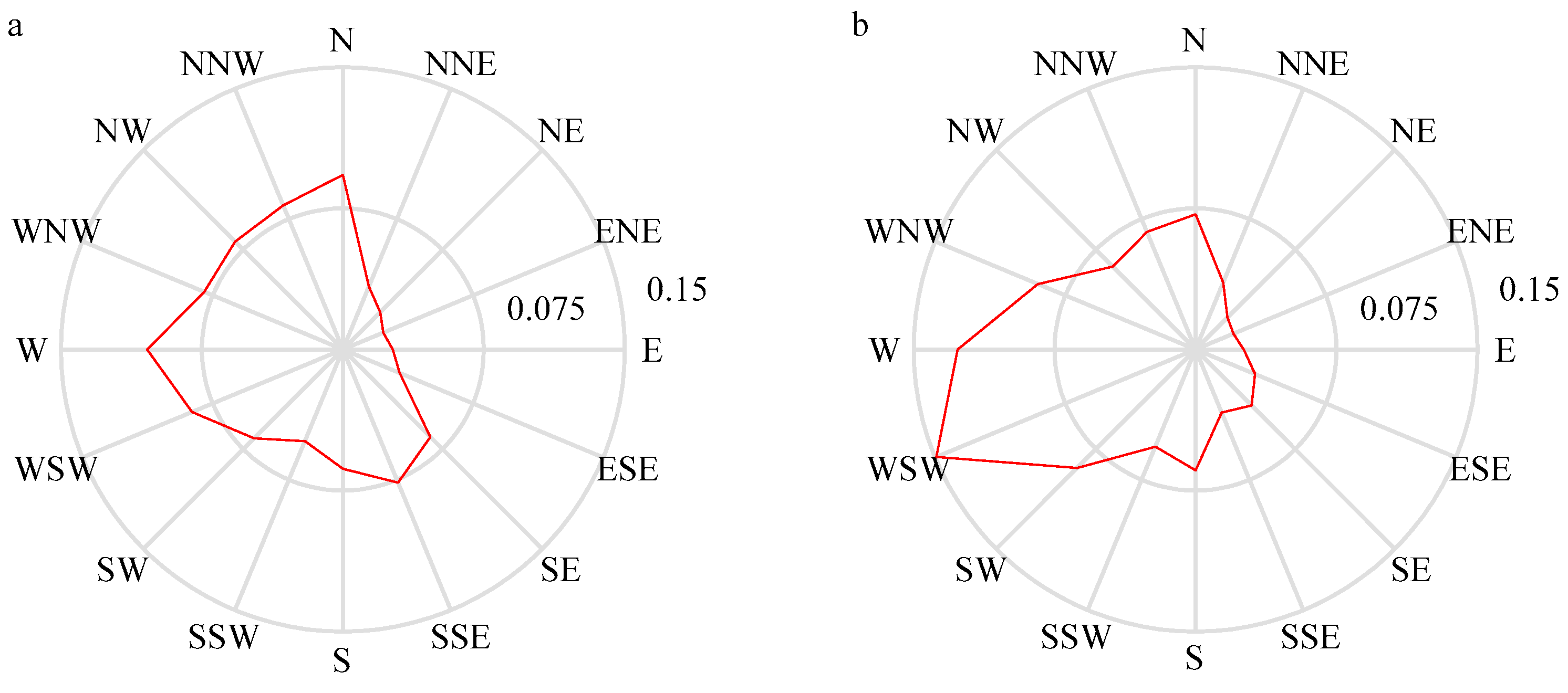
Figure 2 shows that the wind direction rose at a height of 70 m (Figure 2a) and the wind energy rose at a height of 70 m (Figure 2b). As shown in Figure 2, wind direction 1, 8, and 13 (N, SSE, and W) had a large wind direction frequency of 9.28%, 7.66%, and 10.41%, respectively, while wind direction 12 (WSW) had a large wind power density frequency (Figure 2b) of 14.92%. Therefore, in order to investigate their internal correspondence, we needed to study the wind speed characteristics under different wind directions and investigate their characteristics.
Figure 3 was obtained by numerical calculation of the circular variable, which was measured at a height 70 m. Figure 3a shows the wind direction distributions, and Figure 3b depicts the probability distribution of the angular variable ζ. It can be seen from the histogram of the measured wind direction data in Figure 3a that there were up to four main wind directions; therefore, the FVMF with M = 2, M = 3, and M = 4 was chosen to fit the wind direction distribution. Figure 3b illustrates that there were two distinct peaks in the histogram of the angular variable ζ; Therefore, the FVMF with M = 2 was selected to construct the probability distribution of the angular variable ζ. The parameters in the wind direction distributions, the corresponding R2 coefficient, and AIC are shown in Table 2. The parameters in the angular variable ζ distribution function and the corresponding R2 coefficient are shown in Table 3. From Figure 3a and Table 2, it can be seen that the FVMF with M = 4 was the best fitted model for the wind direction data. In addition, in order to estimate the parameters of the FVMF model, we redefined sin ( μ m ) and cos ( μ m ) instead of μ m . Here, the μ m should be calculated by sin ( μ m ) and cos ( μ m ) to describe the mean wind direction. The FVMF with M = 4 reflected that the most dominant wind direction was 4.69 rad (268.6°). As displayed in Figure 3b and Table 3, the FVMF with M = 2 was suitable to describe the angular variable ζ distribution.
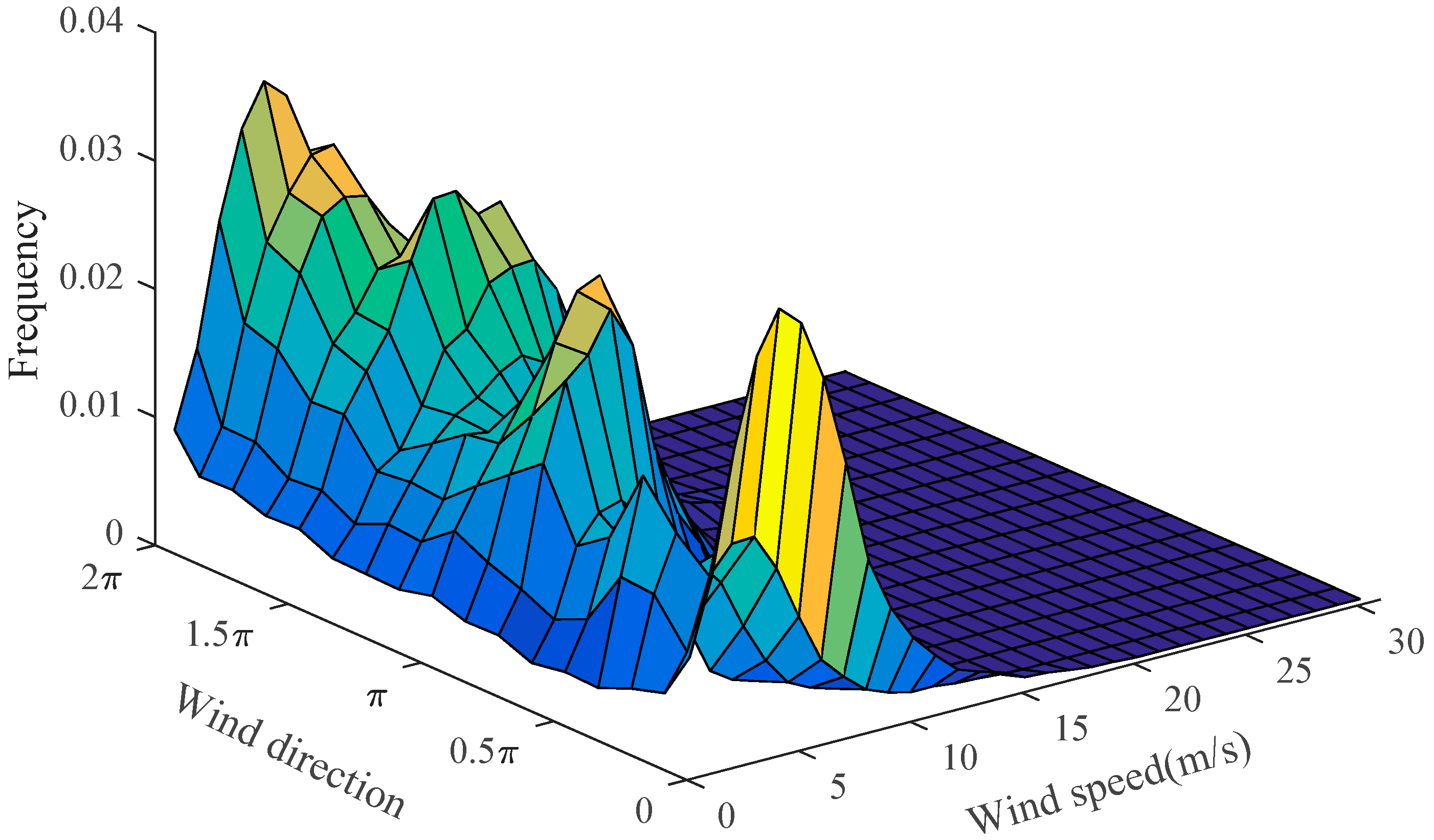
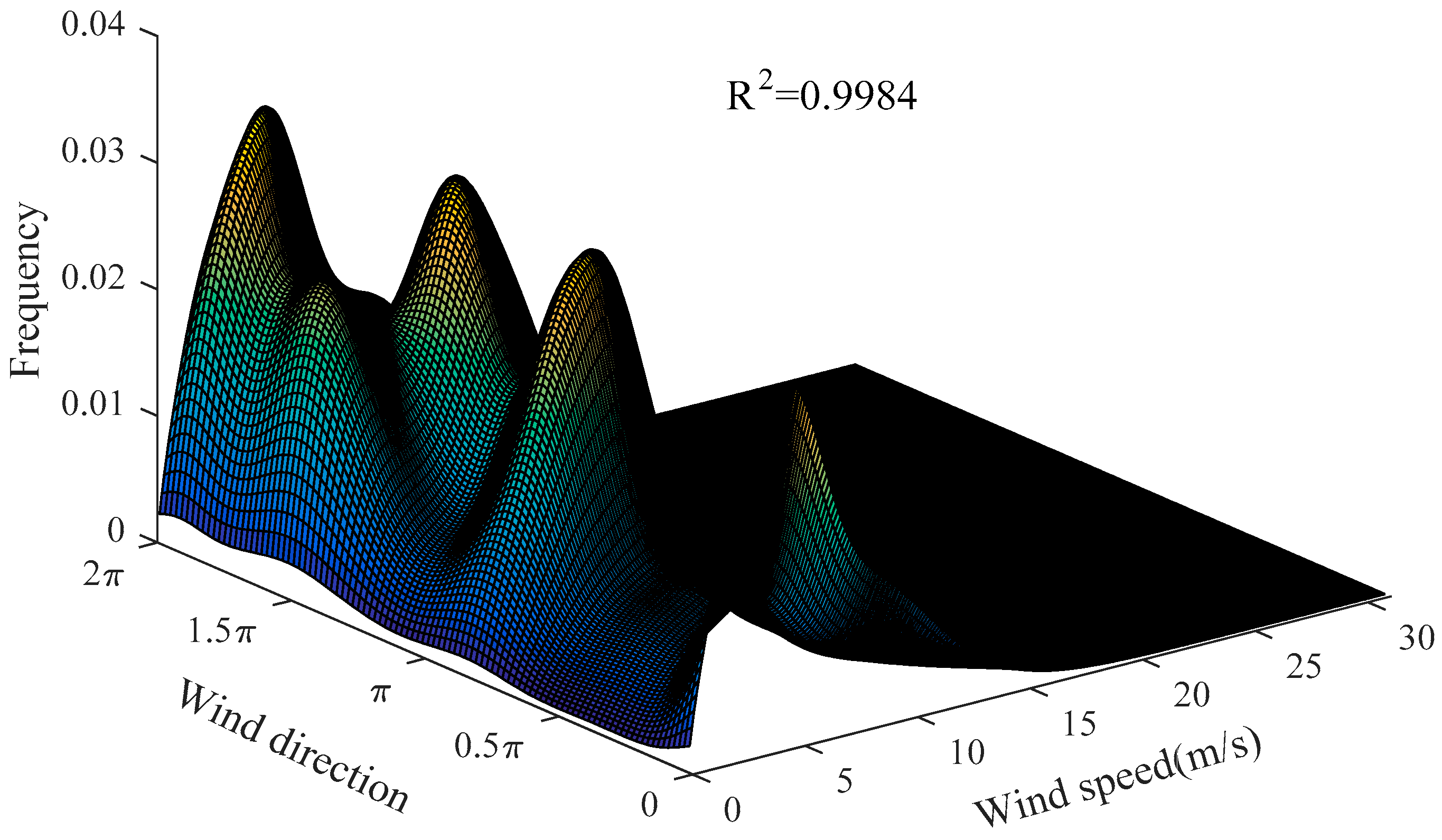
Figure 4 shows the joint probability distribution of actual wind direction and speed at a height of 70 m. Figure 5 shows the joint probability distribution at a height of 70 m, which was obtained with the angular–linear distribution model. According to the proposed joint probability distribution at a height 70 m, the wind speed distribution under 16 wind directions could be determined. The corresponding R2 value can be seen in Table 4. As can be seen from Figure 4 and Figure 5 and Table 4, the proposed model had a great degree of fit to the sample data at a height 70 m. Moreover, in order to verify the validity of the selected model, the proposed model was used to construct the joint probability distribution at a height of 50 m. It should be borne in mind that the wind direction varied slightly from 70 m to 50 m.
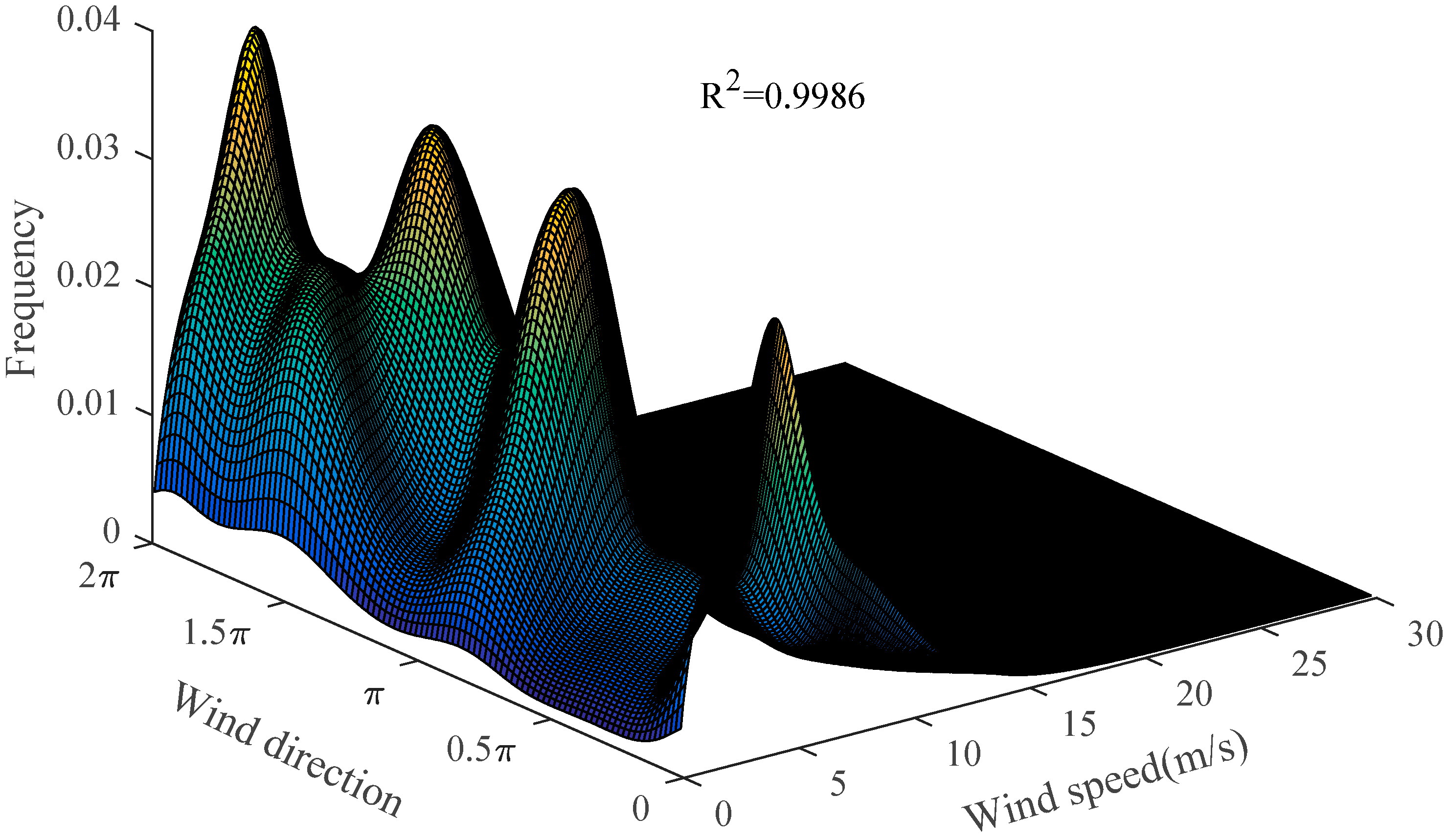
Figure 6 shows the joint probability distribution at a height of 50 m. In the proposed joint distribution model, W–L distribution was selected to process the wind speed data, and the FVMF with M = 4 was the fitted model for the wind direction data. Moreover, the FVMF with M = 2 was chosen to describe the angular variable ζ distribution. The parameters in the joint probability distribution at a height of 50 m and the corresponding R2 coefficient are shown in Table 5. According to the proposed joint probability distribution at a height of 50 m, the wind speed distribution under 16 wind directions could be determined. The corresponding R2 value can be seen in Table 6. It can be seen from the above analysis that the proposed model could well present wind characteristics at different heights.
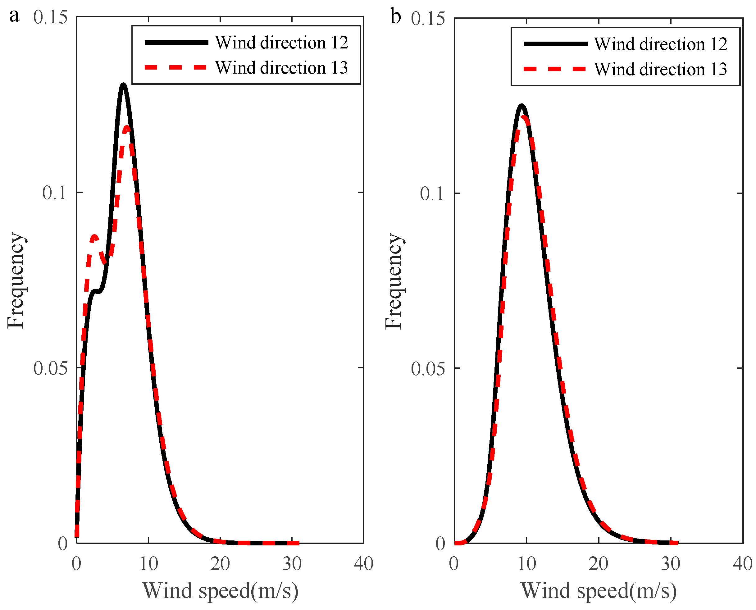
The wind direction was recorded in 16 intercardinal directions. Each wind direction of the 16 intercardinal directions had a corresponding wind speed and a wind power density distribution. Due to the limitation of space, we have only given the results of two wind directions—wind direction 12 (E) and wind direction 13 (W)—in Figure 7. The figure was drawn by applying the joint probability density distribution at a height of 70 m. As can be seen from Figure 7, the most probable wind speeds for wind direction 12 and 13 were 6.5 m/s and 6.95 m/s, respectively; the wind speeds carrying maximum energy were 9.34 m/s and 9.63 m/s, respectively.
The FVMF with M = 4 was a good fitted model for the wind direction data and could be used to investigate the wind direction characteristics for four seasons. The four seasons were defined as follows: (a) spring: March, April, and May; (b) summer: June, July, and August; (c) Autumn: September, October, and November; (d) winter: December, January, and February. Figure 8 depicts the wind direction distributions over four seasons. It was drawn using the wind direction data of 70 m for three years. The parameters in the wind direction model over four seasons and the corresponding R2 coefficient are shown in Table 7. As can be seen from Figure 8, the most dominant wind direction was 5 rad (286.6°) in the spring season, 6 rad (348.8°) in the summer season, 4.5 rad (260.2°) in the autumn season, and 4.7 rad (267.1°) in the winter season. There were more than two prevailing directions in the four seasons. It was concluded from Figure 8 that the wind direction had seasonal features.

7. Conclusions

This paper presents the analysis of wind speed and wind direction using joint probability distribution methods. The joint distribution was obtained with wind direction and speed distributions. By fitting the wind data at different heights, the proposed model could well present wind characteristics. Thus, the proposed model was used to investigate the wind direction and wind speed. The main findings of this paper are as follows:
(1) W–W, L–L, and W–L distribution with higher R2 coefficient provide a good fitting for wind speed data at a height of 70 m. In this paper, the best fitting model for wind speed was W–L distribution, which could accurately represent wind speed characteristics.
(2) The FVMF with M = 4 was a good fitted model for the wind direction data at a height of 70 m and could accurately describe the wind direction distribution with multiple peaks. Moreover, the dominant wind direction was 4.69 rad (268.6°) in the three years.
(3) The joint probability distribution provided a good fit to the measured wind data at different heights, and the R2 of the joint probability distribution was greater than 0.99, indicating that this model was able to explain more than 99% of wind data. With the joint probability distribution, the most probable wind speeds for wind direction 12 and 13 were 6.5 m/s and 6.95 m/s at a height of 70 m, respectively; the wind speed carrying maximum energy were 9.34 m/s and 9.63 m/s at a height of 70 m, respectively.
(4) The wind direction had seasonal features. The most dominant wind direction was 5 rad (286.6°) in the spring season, 6 rad (348.8°) in the summer season, 4.5 rad (260.2°) in the autumn season, and 4.7 rad (267.1°) in the winter season. Moreover, there were more than two prevailing directions in the four seasons.

Author Contributions

Data curation, Q.L.; Formal analysis, Q.L.; Investigation, Y.G.; Methodology, Y.G. and Z.Y.; Project administration, L.Z. (Lidong Zhang); Resources, L.Z. (Lei Zhang); Software, Q.L. and L.Z. (Lei Zhang); Supervision, L.Z. (Lidong Zhang) and L.Z. (Lei Zhang); Validation, Y.G. and Z.Y.; Writing—original draft, L.Z. (Lidong Zhang) and Q.L.; Writing—review & editing, all the authors.

Funding

This work was funded by the National Natural Science Foundation of China [51607177, 61433012, U1435215]; the Science and Technology Development Projects of Jilin city, China [No. 201750203]; the Development of Education of Jilin Province, China [No. JJKH20180435KJ]; and the China Postdoctoral Science Foundation (2018M631005).

Acknowledgments

We would like to thank Jilin Tongli Wind Power Co. LTD for helping us to collect the data.

Conflicts of Interest

The authors declare no conflict of interest.

References

  1. Masseran, N.; Razali, A.M.; Ibrahim, K.; Zin, W.W. Evaluating the wind speed persistence for several wind stations in Peninsular Malaysia. Energy 2012, 37, 649–656. [Google Scholar] [CrossRef]
  2. Amjady, N.; Abedinia, O. Short term wind power prediction based on improved Kriging interpolation, empirical mode decomposition, and closed-loop forecasting engine. Sustainability 2017, 9, 2104. [Google Scholar] [CrossRef]
  3. Dai, K.; Bergot, A.; Liang, C.; Xiang, W.N.; Huang, Z. Environmental issues associated with wind energy—A review. Renew. Energy 2015, 75, 911–921. [Google Scholar] [CrossRef]
  4. Shifeng, W.; Sicong, W. Impacts of wind energy on environment: A review. Renew. Sustain. Energy Rev. 2015, 49, 437–443. [Google Scholar]
  5. Zhao, H.; Zhao, H.; Guo, S. Short-Term Wind Electric Power Forecasting Using a Novel Multi-Stage Intelligent Algorithm. Sustainability 2018, 10, 881. [Google Scholar] [CrossRef]
  6. Carta, J.A.; Ramírez, P.; Bueno, C. A joint probability density function of wind speed and direction for wind energy analysis. Energy Convers. Manag. 2008, 49, 1309–1320. [Google Scholar] [CrossRef]
  7. Wang, J.; Hu, J.; Ma, K. Wind speed probability distribution estimation and wind energy assessment. Renew. Sustain. Energy Rev. 2016, 60, 881–899. [Google Scholar] [CrossRef]
  8. Zhang, J.; Wei, Y.; Tan, Z.; Wang, K.; Tian, W. A hybrid method for short-term wind speed forecasting. Sustainability 2017, 9, 596. [Google Scholar] [CrossRef]
  9. Shu, Z.R.; Li, Q.S.; Chan, P.W. Investigation of offshore wind energy potential in Hong Kong based on weibull distribution function. Appl. Energy 2015, 156, 362–373. [Google Scholar] [CrossRef]
  10. Pishgar-Komleh, S.H.; Keyhani, A.; Sefeedpari, P. Wind speed and power density analysis based on weibull and rayleigh distributions (a case study: Firouzkooh county of Iran). Renew. Sustain. Energy Rev. 2015, 42, 313–322. [Google Scholar] [CrossRef]
  11. Masseran, N.; Razali, A.M. Modeling the wind direction behaviors during the monsoon seasons in peninsular Malaysia. Renew. Sustain. Energy Rev. 2016, 56, 1419–1430. [Google Scholar] [CrossRef]
  12. Johnson, R.A.; Wehrly, T.E. Some angular-linear distributions and related regression models. J. Am. Stat. Assoc. 1978, 73, 602–606. [Google Scholar] [CrossRef]
  13. Erdem, E.; Shi, J. Comparison of bivariate distribution construction approaches for analysing wind speed and direction data. Wind Energy 2011, 14, 27–41. [Google Scholar] [CrossRef]
  14. Ye, X.W.; Xia, P.S.; Su, Y.H.; Chen, B. Analysis and probabilistic modeling of wind characteristics of an arch bridge using structural health monitoring data during typhoons. Struct. Eng. Mech. 2017, 63, 809–824. [Google Scholar]
  15. Manwell, J.F.; Mccowan, J.G.; Rogers, A.L. Wind Energy Explained: Theory, Design and Application, Second Edition; John Wiley & Sons: New York, NY, USA, 2010. [Google Scholar]
  16. Goyal, P.K.; Datta, T.K. Effect of wind directionality on the vulnerability of rural houses due to cyclonic wind. Nat. Hazards Rev. 2013, 14, 258–267. [Google Scholar] [CrossRef]
  17. Han, Q.; Hao, Z.; Hu, T.; Chu, F. Non-parametric models for joint probabilistic distributions of wind speed and direction data. Renew. Energy 2018, 126, 1032–1042. [Google Scholar] [CrossRef]
  18. Islam, M.R.; Saidur, R.; Rahim, N.A. Assessment of wind energy potentiality at kudat and labuan, malaysia using weibull distribution function. Energy 2011, 36, 985–992. [Google Scholar] [CrossRef]
  19. Sedaghat, A.; Hassanzadeh, A.; Jamali, J.; Mostafaeipour, A.; Chen, W.H. Determination of rated wind speed for maximum annual energy production of variable speed wind turbines. Appl. Energy 2017, 205, 781–789. [Google Scholar] [CrossRef]
  20. Tian, P.C. Estimation of wind energy potential using different probability density functions. Appl. Energy 2011, 88, 1848–1856. [Google Scholar]
  21. Carta, J.A.; Ramírez, P.; Velázquez, S. A review of wind speed probability distributions used in wind energy analysis: Case studies in the Canary Islands. Renew. Sustain. Energy Rev. 2009, 13, 933–955. [Google Scholar] [CrossRef]
  22. Masseran, N.; Razali, A.M.; Ibrahim, K.; Zaharim, A.; Sopian, K. The probability distribution model of wind speed over east malaysia. Res. J. Appl. Sci. Eng. Technol. 2013, 6, 1774–1779. [Google Scholar] [CrossRef]
  23. Jaramillo, O.A.; Borja, M.A. Bimodal versus weibull wind speed distributions: An analysis of wind energy potential in La Venta, Mexico. Wind Eng. 2009, 28, 225–234. [Google Scholar] [CrossRef]
  24. Kollu, R.; Rayapudi, S.R.; Narasimham, S.; Pakkurthi, K.M. Mixture probability distribution functions to model wind speed distributions. Int. J. Energy Environ. Eng. 2012, 3, 27. [Google Scholar] [CrossRef] [Green Version]
  25. Jones, R.H.; Daniels, A.; Bach, W. Fitting a circular distribution to a histogram. J. Appl. Meteorol. 2010, 15, 94–97. [Google Scholar] [CrossRef]
  26. Carta, J.A.; Bueno, C.; Ramírez, P. Statistical modelling of directional wind speeds using mixtures of von mises distributions: Case study. Energy Convers. Manag. 2008, 49, 897–907. [Google Scholar] [CrossRef]
  27. Masseran, N.; Razali, A.M.; Ibrahim, K.; Latif, M.T. Fitting a mixture of von mises distributions in order to model data on wind direction in peninsular Malaysia. Energy Convers. Manag. 2013, 72, 94–102. [Google Scholar] [CrossRef]
  28. Erdem, E.; Shi, J. ARMA based approaches for forecasting the tuple of wind speed and direction. Appl. Energy 2011, 88, 1405–1414. [Google Scholar] [CrossRef]
  29. Heckenbergerova, J.; Musilek, P.; Krömer, P. Optimization of Wind Direction Distribution Parameters Using Particle Swarm Optimization. Adv. Intell. Syst. Comput. 2015, 334, 15–26. [Google Scholar]
  30. Williams, B.; Christensen, W.F.; Rees, C.S. Pollution source direction identification: Embedding dispersion models to solve an inverse problem. Environmetrics 2015, 22, 962–974. [Google Scholar] [CrossRef]
  31. Gatto, R. Some computational aspects of the generalized von mises distribution. Stat. Comput. 2008, 18, 321–331. [Google Scholar] [CrossRef]
  32. Calderara, S.; Prati, A.; Cucchiara, R. Mixtures of von mises distributions for people trajectory shape analysis. IEEE Trans. Circuits Syst. Video Technol. 2011, 21, 451–471. [Google Scholar] [CrossRef]
  33. Zhang, S.; Jin, J. Computation of special functions. Am. J. Phys. 1997, 65, 355. [Google Scholar] [CrossRef]
  34. Mcgraw, T.; Vemuri, B.C.; Yezierski, B.; Mareci, T. Von mises-fisher mixture model of the diffusion odf. In Proceedings of the IEEE International Symposium on Biomedical Imaging: From Nano to Macro, Arlington, VA, USA, 6–9 April 2006; pp. 65–68. [Google Scholar]
  35. Koeppl, G.W. Putnam’s Power from the Wind; Van Nostrand Reinhold: New York, NY, USA, 1982. [Google Scholar]
  36. Spera, D.A. Wind turbine technology. Am. Soc. Mech. Eng. 1994, 31, 1561–1572. [Google Scholar]
  37. Carta, J.A.; Mentado, D. A continuous bivariate model for wind power density and wind turbine energy output estimations. Energy Convers. Manag. 2007, 48, 420–432. [Google Scholar] [CrossRef]
  38. Jamil, M.; Parsa, S.; Majidi, M. Wind power statistics and an evaluation of wind energy density. Renew. Energy 1995, 6, 623–628. [Google Scholar] [CrossRef]
  39. Adaramola, M.S.; Agelin-Chaab, M.; Paul, S.S. Assessment of wind power generation along the coast of Ghana. Energy Convers. Manag. 2014, 77, 61–69. [Google Scholar] [CrossRef]
  40. Mathew, S.; Pandey, K.P.; Anil, K.V. Analysis of wind regimes for energy estimation. Renew. Energy 2002, 25, 381–399. [Google Scholar] [CrossRef]
Figure 1. The distribution of wind speed characteristics at a height of 70 m: (a) wind speed distributions, (b) probability distribution of wind power density.
Sustainability 10 04338 g001
Figure 2. The rose diagrams at a height of 70 m: (a) wind direction rose; (b) wind energy rose.
Sustainability 10 04338 g002
Figure 3. The fitting of the finite mixture of von Mises function for the circular variable: (a) wind direction distributions; (b) probability distribution of the angular variable ζ.
Sustainability 10 04338 g003
Figure 4. The joint probability distribution of actual wind direction and speed at a height of 70 m.
Sustainability 10 04338 g004
Figure 5. The joint probability distribution at a height of 70 m.
Sustainability 10 04338 g005
Figure 6. The joint probability distribution at a height of 50 m.
Sustainability 10 04338 g006
Figure 7. The distribution of wind speed characteristics at a height 70 m: (a) wind speed distributions under different wind directions; (b) probability distributions of wind power density under different wind directions.
Sustainability 10 04338 g007
Figure 8. The wind direction distributions over four seasons.
Sustainability 10 04338 g008
Table 1. Fitted parameters in wind speed distributions.
Distributionm w m α m / μ m β m ( m / s ) / σ m R2AIC
Weibull–Weibull10.53827.48952.46390.99421073705
20.46176.03981.5558
Lognormal–Lognormal10.77941.84370.43420.99451079551
20.22060.81390.8520
Weibull–Lognormal10.75946.10161.77900.99431073344
20.24052.04130.3324
Table 2. Fitted parameters in wind direction models.
Distributionm w m k m sin ( μ m ) cos ( μ m ) R2AIC
FVMF with M = 210.86040.7638−0.93150.36390.9890740279
20.13966.77580.4512−0.8924
FVMF with M = 310.24145.2855−0.9904−0.13790.9883737192
20.35872.7048−0.32280.9465
30.39991.65290.3105−0.9506
FVMF with M = 410.19995.20580.4319−0.90190.9864735538
20.15678.3011−0.14140.9900
30.56101.5859−0.9997−0.0263
40.08252.78120.94080.3388
Table 3. Fitted parameters in angular variable ζ.
Distributionm w m k m sin ( μ m ) cos ( μ m ) R2
FVMF with M = 210.25440.9229−0.08560.99630.9906
20.74560.42960.9019−0.4318
Table 4. The R2 value of the 70-m high wind speed distribution under 16 wind directions.
Wind DirectionNNNENEENEEESESESSES
R20.98310.91220.9090.93410.91370.93540.97990.99970.9886
Wind DirectionSSWSWWSWWWNWNWNNW
R20.98530.99580.9710.98480.9970.9850.9869
Table 5. Fitted parameters in the joint probability distribution at a height of 50 m.
Distributionm w m α m / μ m β m ( m / s )   /   σ m k m sin ( μ m ) cos ( μ m ) R2
W–L10.6108 5.3568 1.6104 0.9933
20.3892 1.8266 0.3853
FVMF with M = 410.1999 0.1999 5.2058 0.4319 0.9864
20.1567 0.1567 8.3011 −0.1414
30.5610 0.5610 1.5859 −0.9997
40.0825 0.0825 2.7812 0.9408
FVMF with M = 210.4410 0.6048 −0.1081 0.9941 0.9903
20.5590 0.6030 0.8675 −0.4974
Table 6. The R2 value of the 50-m high wind speed distribution under 16 wind directions.
Wind DirectionNNNENEENEEESESESSES
R20.98680.92880.90330.91390.93370.94680.97290.98350.9835
Wind DirectionSSWSWWSWWWNWNWNNW
R20.98080.99550.97370.98570.99810.98820.9896
Table 7. Fitted parameters in wind direction models over four seasons.
SeasonDistributionm w m k m sin ( μ m ) cos ( μ m ) R2
SpringFVMF with M = 410.16406.86740.3582−0.93360.9871
20.03097.40650.98510.1721
30.74881.0602−0.95800.2869
40.056323.9653−0.05760.9983
SummerFVMF with M = 410.37521.0583−0.9999−0.01000.9873
20.31263.42640.5993−0.8005
30.24924.6498−0.13680.9906
40.06306.43720.86260.5058
AutumnFVMF with M = 410.41613.1634−0.9855−0.16960.9859
20.05993.43600.94560.3254
30.29504.51230.3778−0.9259
40.22906.5931−0.21470.9767
WinterFVMF with M = 410.08038.51410.4261−0.90470.984
20.03104.00850.95290.3031
30.79661.5032−0.9989−0.0477
40.092222.7153−0.07080.9975

