Simulation-Optimization Approach for the Logistics Network Design of Biomass Co-Firing with Coal at Power Plants

Abstract

This work proposes a hybrid scheme that combines a simulation model and a mathematical programming model for designing logistic networks for co-firing biomass, specifically switchgrass, in conventional coal-fired power plants. The advantages of co-firing biomass include: (1) the creation of green jobs; (2) the efficient use of current power plant infrastructure; (3) fostering the penetration of renewable energy into power networks; and, (4) the reduction of greenhouse gas (GHG) emissions. The novelty of this work lies in the inclusion of (1) the inherent variability of biomass supply at the parcel level, and (2) the effects of climate change on future biomass supply when designing a feedstock logistic network. The design optimization is conducted at the farm/parcel level (most, if not all, previous works have used county level average data) and integrates the crop growth predictions employing United States Department of Agriculture’s (USDA’s) Agricultural Land Management with Numerical Assessment Criteria (ALMANAC) simulation model; the output of the simulations is input into the mixed integer linear programming (MILP) hub-and-spoke model to minimize the overall cost of the logistic network. Specifically, the MILP-based model selects the parcels and depot locations as well as biomass transportation flows by taking into consideration different types of soil, land cover characteristics, and predicted yields, which account for both historical and forecasted weather data. The hybrid methodology was tested by solving realistic situations, which considered varying weather conditions. The gross results indicate that the optimized logistic network enabled meeting a 20% biomass co-firing rate demand, which reduced 1,158,867 Mg per year in GHG emissions by co-firing with biomass.

1. Introduction

Coal-fired power plants generate one-third of the electricity in the United States [1]. The greenhouse gas (GHG) emissions that were produced from these power plants can be reduced by co-firing with biomass. Biomass co-firing entails replacing a portion of the coal used in the power plant with biomass to reduce the net GHG emissions. Noteworthy, biomass provides substantial environmental benefits, such as net zero emissions when burned for energy production [2]. Thus, co-firing biomass with coal can reduce GHG emissions without incurring major plant infrastructure changes/investments, while benefiting the local economy by creating agricultural and transportation jobs. The co-firing rate, defined as the ratio of the biomass to the coal mass used in the power plant operations, must be between 10% and 25% to avoid degrading the thermal efficiency of the power plant and to keep plant infrastructure unaltered [3].

For biomass to be a viable solution for reducing GHG emissions, and for it to compete against fossil fuels, its feedstock supply chain (SC) must be efficient and all of its relevant associated costs should be minimized. To attain such objectives, this paper presents a hybrid computational method that combines crop growth simulations to predict biomass yields at the parcel level and a Mixed-Integer Linear Programming (MILP) hub-and-spoke network model to address the problem of designing logistic biomass SCs for biomass co-firing in coal-fired power plants. The proposed hybrid method combines simulation, to determine the biomass yield at a farm/parcel level, and a MILP model to optimize the logistics network. Firstly, the biomass yield simulations are executed utilizing the United States Department of Agriculture’s (USDA’s) Agricultural Land Management with Numerical Assessment Criteria (ALMANAC) [4] software. ALMANAC is a comprehensive simulation model that predicts plant yield in multiple locations when considering heterogeneous climatic conditions (refer to Section 4: Case Study). Secondly, the biomass yield is fed to a tailored hub-and-spoke model to design an optimal supply chain network.

The contributions of this research are multifaceted, including: modeling, methodology, and application. Regarding modeling, a MILP hub-and-spoke model for biomass co-firing in coal fired-power plants is proposed. This model considers the biomass yield variability under climate change scenarios and refines the analysis of biomass yield/availability for future scenarios. A methodology is presented to estimate the biomass yield in future instances under climate change conditions. With respect to application, a realistic case study in a coal power plant in South Texas with a 20% co-firing rate demand is presented.

This paper is structured as follows. Section 2 reviews previous works and highlights gaps in the literature. Section 3 presents the proposed MILP hub-and-spoke model formulation. Section 4 presents the data used to construct the realistic case study and instances. The results of our case study are presented in Section 5. Lastly, concluding remarks are provided along with recommendations for future work in Section 6.

2. Literature Review

This section reviews previous analytical models for optimizing biomass supply chains for co-firing in coal power plants. Ba et al. [5] provides an in-depth literature review, explaining common concepts in supply chain networks, as well as their designs, strengths, and weaknesses. Ba et al. [5] highlighted unaddressed challenges in biomass models, such as: (1) the large-scale nature of the problem; (2) the use of different commercial solvers, which lead to difficult reproduction of results; (3) the fact that most modeling approaches show limited temporal and spatial granularity; and, (4) the limitation that comes from many fixed network supply chains, where the model is unable to choose the harvesting location. Noteworthy, Ba et al. [5] pointed out that there is a lack of industrial and operations research perspective in the bioenergy SC network design problem.

Roni et al. [6] proposed a hub-and-spoke model to optimize the SC of biomass for co-firing. A Long-haul delivery of biomass in large volumes was considered, as the SC covered most of the United States. Their model is an extension of the hub-and-spoke design problem, which included a step-wide cost function that better represented transportation costs. They were able to determine that biomass that was located within a 75-mile radius of the power plant had a transportation cost of $8.53/dry ton. As explained by Roni et al. if the biomass was located outside the 75-mile radius, co-firing no longer becomes a viable solution. Therefore, Roni et al. indicate that the closer the biomass supply is to the power plant, the more economically competitive co-firing biomass becomes. Additionally, similar findings can be seen in woody biomass procurement studies done by Kizha et al. [7], where results from their case study in northern California point to how proximity to the feedstock supply to the power plant create competitive advantages when compared to farther sources. Noteworthy, Kizha et al. discuss how competition may be further intensified by the entry of an additional biomass consumer. Therefore, adding more detail to the biomass SC, such as parcel selection in a local agricultural setting, allows for a more comprehensive analysis and it potentially lowers the costs of the biomass SC.

Poudel et al. [8] used a two-stage stochastic model to manage a biomass SC network. The model considers the design and management of a biomass co-firing SC that is subject to feedstock supply uncertainty. The output of their model provided season-wide utilization of multi-model facilities, the optimal number of containers transported between the multi-model facilities, and the amount of biomass processed, stored, and transported from multiple supply sites to coal power plants when considering biomass supply uncertainty. A case study with data from Mississippi and Alabama counties was analyzed. Results show that high feedstock variability increases the unit delivery cost by $1.87/ton. Poudel et. al address the uncertainty of biomass supply in order to deliver the biomass to the power plants, but the optimization of the SC is limited the depot-to-plant arcs, and farm locations were not considered.

Regarding time-dependent variables that produce impacts on the energy generation cost, Akgul et al. [9] formulated a mixed-integer nonlinear programming model of carbon negative energy generation in the UK to examine the potential for existing power generation assets to act as a carbon sink as opposed to a carbon source. Using a Pareto front-based approach, Akgul et al. [9] analyzed the technical and economic compromises of transitioning from a dedicated fossil-fuel-only power network to a carbon negative electricity generation network. The relative fuel cost was a key determinant of the required carbon price in the model. They also found that increasing the biomass availability reduced the cost of generating carbon negative electricity. The authors investigated three different scenarios (low, central, and high prices for CO₂ and coal) for three years: 2012, 2020, and 2050. Their results indicate that CO₂ prices must be within the range of £120–£175/ton to incentivize the generation of carbon negative electricity. Thus, increasing the availability of biomass was found to be critical for reducing this cost. This conclusion incentivizes the need to develop models to increase the cost effectiveness of bioenergy SCs.

Roni et al. [10] focused on studying a long-haul rail transportation network, since, in practice, many power plants receive coal through trains and tend to be close to railway stations. They considered a supply of 100 million tons of biomass within 50 miles of the power plants. In their model, trucks were considered for transporting biomass in shorter distances. Roni et al.’s network begins at depot’s (or storage) locations and end in the co-firing power plant. Roni et al.’s model aims to optimize the SC by reducing transportation costs, increasing production rates, and decreasing moisture in harvested switchgrass. Their work evaluates the following strategies: blending feedstock and integrated landscape management as means to further improve the SC performance of lignocellulosic crops. Roni et al.’s analysis is shown as a high-level overview and it encourages for further investigation in the design of biomass SCs.

De Laporte et al. [11] analyzed three different supply chain scenarios for growing, transporting, and exporting switchgrass in Canada. In their study, two local power plant locations were considered along with international exports, using pellets and bales. The model focused on the price increase relative to the demand increase and did not account for storage costs during off-seasons. The authors concluded that the local transportation model was the most efficient due to policy implementations, demands, and lower costs.

A case study that was conducted by Hart [12], in the Texas area, unveiled that the average switchgrass yield from the 45 soil locations studied is 8.05 metric tons per hectare, with a standard deviation of 3.03; showing switchgrass as the highest yielding biomass when compared to other common sources. Hart found that the optimal solution to the problem studied considers harvesting locations with a biomass yield ranging from 9.74 to 10.70 metric tons per hectare and requires investment in two depot locations (i.e., one in Atascosa and the other in Wilson County). The total cost of the optimal SC network turned out to be $30,828,329, with an emissions reduction of 4.09 × 10⁹ kg of CO₂ per year. Hart’s analysis fails to consider environmental challenges, such as land cover and future climate, as well as a limited set of potential parcels. Taking Hart’s thesis [12] as a reference point for further improvement and analysis, our work attempts to further build upon his research in efforts to create a more comprehensive study. Therefore, his analysis considering cost figures and biomass selection were evaluated as substantial references for our SC network design.

On the basis of the identified gaps and the conclusions that are generated within the aforementioned research works, this paper aims to provide a novel hybrid methodology that integrates a MILP hub-and-spoke model, which considers more granularity in the biomass yield estimation, utilizes mostly open-source software to facilitate the replication and dissemination of results, and optimizes the topology design of the SC networks for biomass co-firing in coal-fired power plants. This work differentiates from previous approaches by adding more granularity to the analysis of biomass availability at the farm/parcel level. This allows for decision makers to determine the layout of the supply chain in detail, determining which parcels will be used and which roads will be used (obtained through the arcs selected and the fastest routes associated with these arcs). The proposed methodology includes the feedstock availability in detail using the ALMANAC simulation, considers climate inputs (historical and future scenarios), and the changing GHG emissions in the atmosphere.

3. Methodology

A hybrid methodology is proposed to address both tactical and strategic decisions in the feedstock logistics network design problem for co-firing biomass. Hybrid models have been employed for different application domains [13,14]. In this paper, the simulation component involves predicting the switchgrass growth, while accounting for soil, location, and weather/climate inputs. The optimization aims to find the optimal supply chain design (i.e., parcel selection, depot location, and biomass transportation) that minimizes the net cost of the feedstock logistics network.

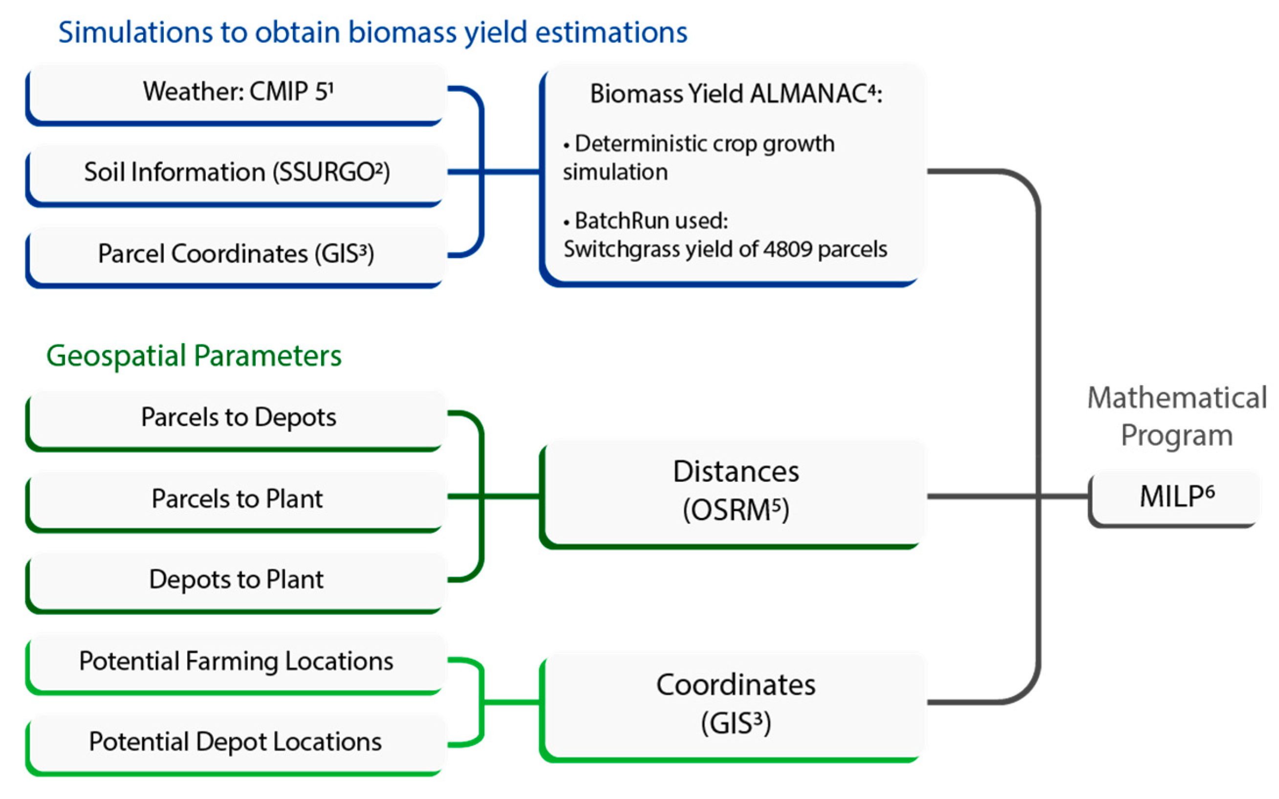
A schematic representation of the hybrid simulation-MILP methodology is shown in Figure 1. The MILP requires two main types of inputs: (1) high-resolution biomass yield and (2) geospatial parameters. The biomass yield is predicted using ALMANAC simulations that consider weather, soil, and location data. The weather and soil inputs (Soil Survey Geographic Database, SSURGO [15]) are outlined in Section 4.3 and Section 4.1.1, respectively. Using the “BatchRun” capabilities of ALMANAC, crop growth in 4908 potential parcels is simulated within the Texas case study presented in Section 4. The geospatial parameters include the potential locations as well as the distances among nodes of the network. The potential locations are obtained by means of Geographical Information System (GIS) data (Section 4). The distances between parcels, depots, and power plant(s) are obtained through shortest route algorithms from the Open Source Routing Machine (OSRM) platform [16]. With all these inputs, the MILP hub-and-spoke model determines the optimal planting and depot locations that take advantage of economies of scale and minimize the net cost of the logistics network while meeting a 20% co-firing rate demand.

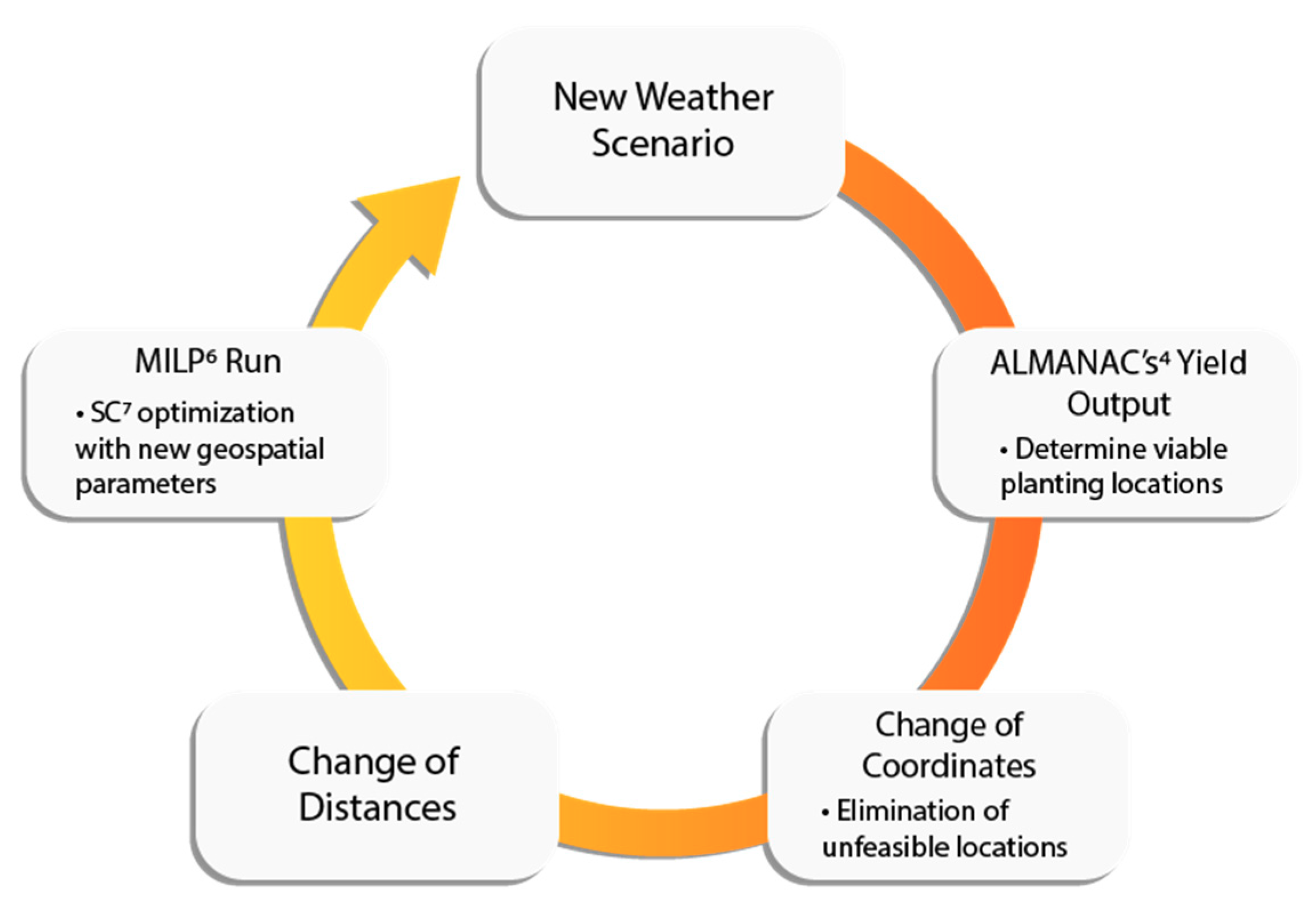
In this paper, we analyze the impact of future weather instances (refer to Figure 2) by running multiple ALMANAC simulations that generate biomass yield estimations and determine viable parcels (planting locations) under future climate conditions. Once the parcels are updated, the coordinates and feasible arcs are updated as well. Subsequently, the MILP model is executed to find the optimal logistics network (Section 4 shows detailed information on inputs and the generation of weather scenarios).

In the next paragraphs, we elaborate on the MILP model and its mathematical formulation. A hub-and-spoke model [19] is proposed for the design and optimization of this biomass cofiring logistics network. Hub-and-spoke networks are present in various industries and they have been a fertile area for interdisciplinary research with applications in terrestrial transportation, airlines, network design, telecommunications, among others [19]. The proposed biomass network consists of three sets of nodes. The first set of nodes represents the parcels. The second set corresponds to the depots (i.e., a facility to wrap, storage, and consolidate biomass bales). The third is the power plant(s). Figure 3 shows a visual representation of a simplified hub-and-spoke model with four parcels, three depot facilities, and one power plant. Figure 3 exemplifies the possible connections between parcels and depots (arcs T1), depots and the power plant (arcs T2), and directly from parcels and the power plant (arcs T3). This optimization model aims to find the parcels to be utilized to grow switchgrass, the necessary depots to serve as storage, and the distribution network that minimizes the overall SC cost.

The definitions of all the parameters used in the MILP formulation follow:

Set Definitions:

$N$ Set of nodes in supply chain network $G\left(N,A\right)$.

$A$ Set of arcs in $G\left(N,A\right)$.

$P$ Set of parcels.

$D$ Set of potential locations for depots.

$C$ Set of coal plants.

$T_1$ Set of arcs that connect parcels to potential depot location.

$T_2$ Set of arcs that connect potential depot to coal plants location.

$T_3$ Set of arcs that connect parcels to coal plants location.

Design Variables:

$X_{ij}$ flow along arc $\left(i,j\right)\in T_1$ from a parcel location to a depot facility.

$Y_{jk}$ flow along arc $\left(j,k\right)\in T_2$ from a depot facility to a coal plant.

$Z_{ik}$ flow along arc $\left(i,k\right)\in T_3$ from a parcel location to a coal plant.

$W_j$ a binary variable which takes the value 1 if j $\in D$ is used as depot, and 0 otherwise.

Problem Parameters:

$c_{ij}^{T_1}$ unit cost charged per metric ton shipped along $\left(i,j\right)\in T_1$.

$c_{jk}^{T_2}$ unit cost charged per metric ton shipped along $\left(j,k\right)\in T_2$.

$c_{ik}^{T_3}$ unit cost charged per metric ton shipped along $\left(i,k\right)\in T_3$.

${\xi }_j$ fixed investment cost to install a depot at node $j\in D$.

$u_j$ represents the storage capacity of depot facility $j\in D$.

$s_i$ represents the supply of biomass at parcel location $i\in P$.

$d_k$ total demand of biomass for electricity production at each coal plant location $k\in C$.

$$Min{\displaystyle \sum }_{i\in P}{\displaystyle \sum }_{j\in D}{c}_{ij}^{T_1}{X}_{ij}+{\displaystyle \sum }_{j\in D}{\displaystyle \sum }_{k\in C}{c}_{jk}^{T_2}{Y}_{jk}+{\displaystyle \sum }_{i\in P}{\displaystyle \sum }_{k\in C}{c}_{ik}^{T_3}{Z}_{ij}+{\displaystyle \sum }_{j\in D}{\xi }_j{W}_j$$

(1)

$$s.t.{\displaystyle \sum }_{\mathrm{j}\in \mathrm{D}}{\mathrm{X}}_{\mathrm{ij}}+{\displaystyle \sum }_{\mathrm{k}\in \mathrm{C}}{\mathrm{Z}}_{\mathrm{ik}}\le {\mathrm{s}}_{\mathrm{i}}\forall \mathrm{i}\in$$

(2)

$${\displaystyle \sum }_{\mathrm{i}\in \mathrm{P}}{\mathrm{X}}_{\mathrm{ij}}-{\displaystyle \sum }_{\mathrm{k}\in \mathrm{C}}{\mathrm{Y}}_{\mathrm{jk}}=0\forall \mathrm{j}\in \mathrm{D}$$

(3)

$${\displaystyle \sum }_{\mathrm{j}\in \mathrm{D}}{\mathrm{Y}}_{\mathrm{jk}}+{\displaystyle \sum }_{\mathrm{i}\in \mathrm{P}}{\mathrm{Z}}_{\mathrm{ik}}={\mathrm{d}}_{\mathrm{k}}\forall \mathrm{k}\in \mathrm{C}$$

(4)

$${\displaystyle \sum }_{\mathrm{j}\in \mathrm{P}}{\mathrm{X}}_{\mathrm{ij}}-{\mathrm{u}}_{\mathrm{j}}{\mathrm{W}}_{\mathrm{j}}\le 0\forall \mathrm{j}\in \mathrm{D}$$

(5)

$${\mathrm{X}}_{\mathrm{ij}}\in {\mathrm{R}}^{+},\forall \left(\mathrm{i},\mathrm{j}\right)\in {\mathrm{T}}_1$$

(6)

$${\mathrm{Y}}_{\mathrm{jk}}\in {\mathrm{R}}^{+},\forall \left(\mathrm{j},\mathrm{k}\right)\in {\mathrm{T}}_2$$

(7)

$${\mathrm{Z}}_{\mathrm{ik}}\in {\mathrm{R}}^{+},\forall \left(\mathrm{i},\mathrm{k}\right)\in {\mathrm{T}}_3$$

(8)

$${\mathrm{W}}_{\mathrm{j}}\in \left\{0,1\right\}\forall \mathrm{j}\in \mathrm{D}$$

(9)

The design variables correspond to flows from parcels to depots, depots to power plants and from parcels to power plants (in metric tons). Moreover, binary variables ($W_j$) are related to depot location selection.

The objective function (1) consists of four terms, which encompass the costs for harvesting, processing, and transporting switchgrass, as well as the cost for opening depots. A breakdown of the costs used in the case study are outlined in Section 4.6. Constraints (2) restrict the supply of biomass for every parcel to the maximum yield. Constraints (3) assure a mass balance in every depot. Constraints (4) assure the biomass demand satisfaction. Constraints (5) set up ensures that the biomass stored is less than the capacity at depots. Constraints (6)–(8) assure a non-negative flow, and (9) are binary constraints for depot location. In the next section, a case of study for the state of Texas is presented.

4. Case Study

To evaluate the applicability of the proposed methodology, a realistic case study is used. This case study corresponds to a local power company located in South-Central Texas, which operates several power plants, including a 1350 MW coal power plant. The power plant consumed approximately 4,563,501 short tons of coal in 2016 [20]. By taking into consideration the energy content of switchgrass and coal, which is 15 and 17.35 MMBtu per short ton, respectively [20,21], it is determined that the energy produced by the coal is 79,176,742 MMBtu. The required switchgrass to produce this same amount of energy is 4,788,535 Mg (metric tons). Finally, taking 20% of the total switchgrass required to match the coal output, the total switchgrass demand ($d_k$) results in 957,707 Mg for a 20% co-firing rate. The next subsections describe the data generation/collection process.

4.1. Biomass Yield

In this section, we describe the procedure that was used to determine the predicted switchgrass yield at the potential parcels through comprehensive simulations. Software and databases used are outlined in detail, including the use of SSURGO [15], ALMANAC [4], and ArcMap [18].

4.1.1. Soil Analysis

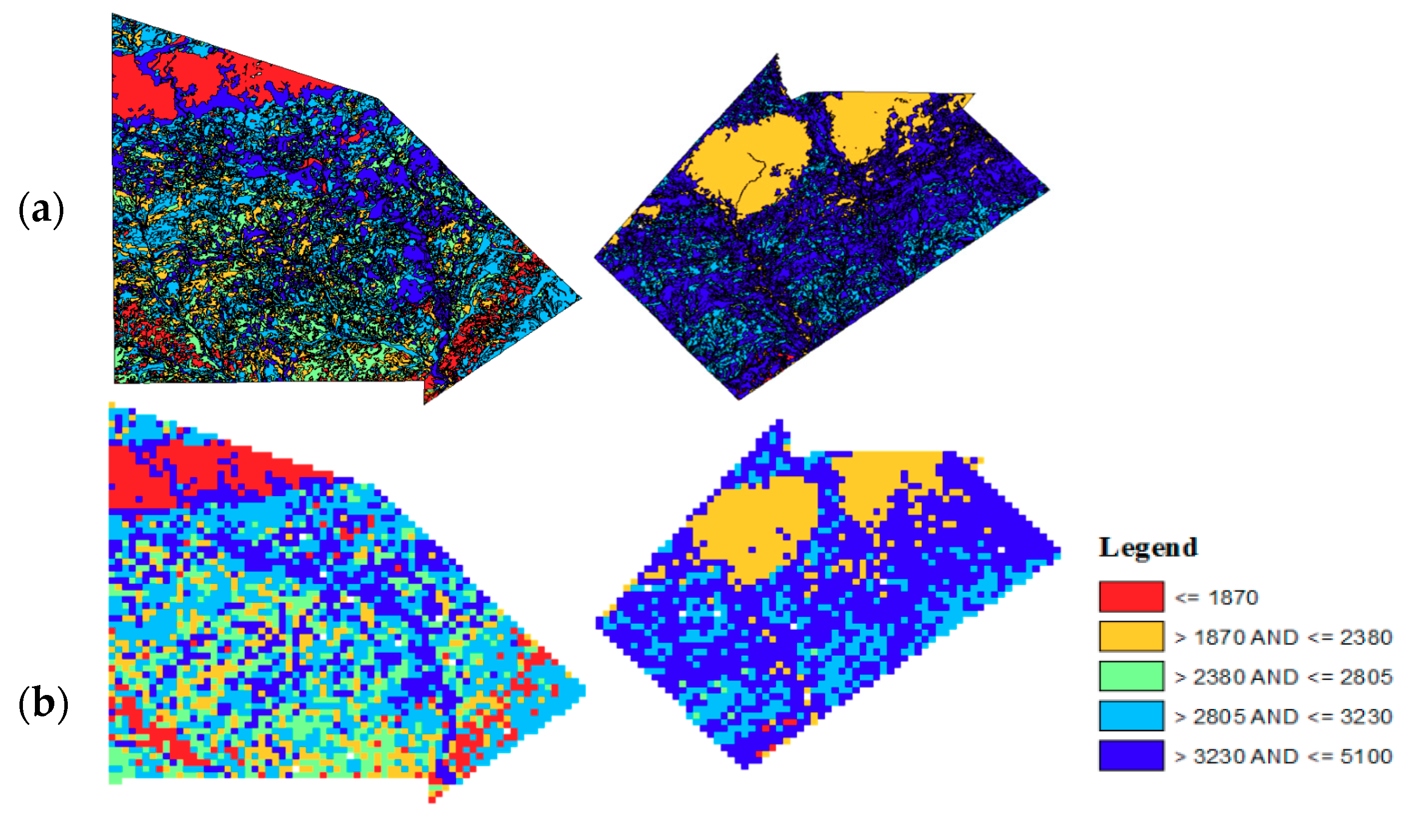
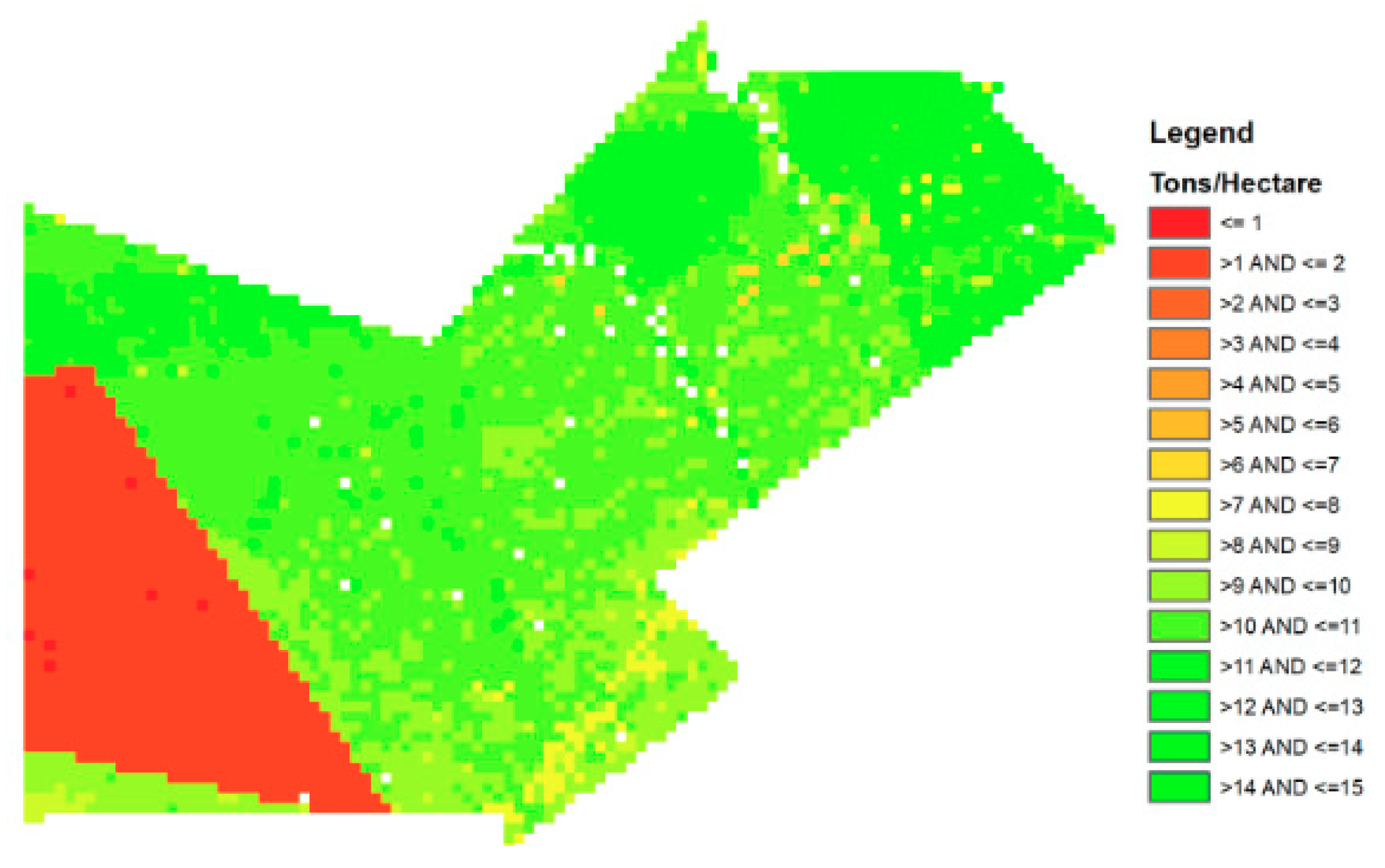
Initially, the counties were divided into parcels. The main challenge faced while defining these parcels was determining if their yield would be comparable to the expected yield for the area. In order to visualize the similarity of the parcel simplification to the original soil data, the USDA’s Soil Survey Geographic Database (SSURGO) [15] maps were used. SSURGO ranks soil types due to its production potential. Due to the large varieties of soil types in the counties, SSURGO’s ranking allows for simpler representation of the soil behavior. The ranking shown in the legend of Figure 4 is for range production potential during a normal precipitation year, which is comparable to switchgrass, for a normal year for the two counties in question.

The soil rank maps were obtained using information from SSURGO and ArcMap mapping capabilities along with the Soil Data Viewer ArcMap extension. The Soil Data Viewer helped to visualize the variety of soil productivity throughout the counties. The soil rank maps were used to create a raster with parcels of 100 hectares each (the size of the parcel was determined to emulate the average size of a farm in the United States, which is approximately 170 hectares and to enhance visualization). The selected size will aid in determining biomass feedstock quantities since the ALMANAC [4] produces an output in metric tons per hectare. The locations used in the crop yield simulation and optimization procedure of the SC are the coordinates from the centroid of each of the 100 hectare parcels.

4.1.2. ALMANAC Analysis

The coordinates determined from the parcel simplification were used to calculate the potential yield of the parcels using ALMANAC ($s_i$). The coordinates from each county were used in separate batch files for various states, such as historical (baseline) and future climate scenarios. The crop used in this ALMANAC-based analysis is Alamo Switchgrass and its corresponding management details. The selection of Alamo Switchgrass was due to its high yield in this area of Texas [12]. The management for Alamo Switchgrass entails initial planting along with fertilizing, and annual collection of the biomass, without hurting the root, allowing for the plant to re-grow the following year without the need to re-plant or fertilize. Additionally, the management did not include irrigation. USDA’s ALMANAC has extensive data for agricultural simulation in the United States. If similar studies were to be done in other areas in the U.S., the yield of the chosen type of biomass can be estimated following this procedure. Moreover, the crops can be ranked to identify the one that provides higher yield in a designated area and this analysis can be done in marginal lands as well. Noteworthy, the proposed approach can be straightforwardly transferable to biofuel and biochemical supply chains.

4.2. Land Cover

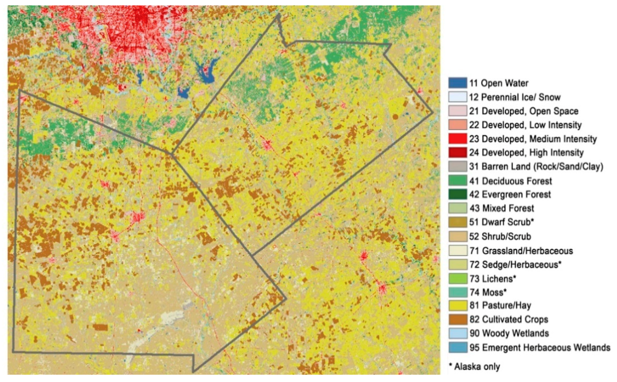
Next, the determination of suitable parcels is described. A feasible parcel allows for the use of land without negatively affecting the environment. In order to account for these environmental obstacles, land cover information was obtained through the National Land Cover Database [22]. The land cover information map is presented in Figure 5.

ALMANAC does not provide yield predictions in uninhabitable parcels (e.g., water bodies or sandy loams) and these areas are not chosen by the model as feasible parcels. The parcels that were discarded are developed areas (21, 22, 23, and 24) and forest areas (41, 42, and 43). The reason to discard forest areas is due to the negative impact that deforestation has in the environment and the communities around it.

4.3. Scenarios

The baseline scenario considers data from 1950 to 2000. The 50 years range allows for a more realistic baseline yield, since it accounts for extreme weather events, such as droughts and floods, among others. Data was collected from the NCDC NOAA database [23] for both counties and encompassed precipitation, minimum daily temperature, and maximum daily temperature. The stations that were used for the baseline scenario are shown in Figure 6. The compiled data did not have enough information to cover the entire period of time. To amend this issue, the ALMANAC’s weather generator was used to fill in any weather data gaps during this period.

Four scenarios of climate change were created. Rainfall and temperature projections from the World Climate Research Programme’s Coupled Model Intercomparison Project Phase 5 (CMIP5) [17] were analyzed. These time series are bias-corrected and statistically downscaled from outputs of general circulation models. A total of 132 daily model outputs of four Representative Concentration Pathways (RCP2.6, RCP4.5, RCP6.0, and RCP8.5) [24] were obtained. Each RCP characterizes a greenhouse gas concentration trajectory adopted in the 5th Assessment Report of the Intergovernmental Panel on Climate Change [25]. The RCP describes a potential future climate with different anthropogenic greenhouse gas emissions, air pollutants, and land use, and it results in radiative forcing values in the year 2100 (2.6 to 8.5 W/m² ~ 490 to 1370 ppm CO₂ equivalent). RCP 8.5 is a baseline scenario and it assumes that emissions will continue to rise throughout the 21st century. RCP6.0 and RCP4.5 assume the greenhouse gas emissions peak around 2080 and 2040, respectively, followed by the reduction of atmospheric discharges. RCP2.6 is the more optimistic scenario, and it assumes very low greenhouse gas emissions, reduced though a series of mitigation strategies.

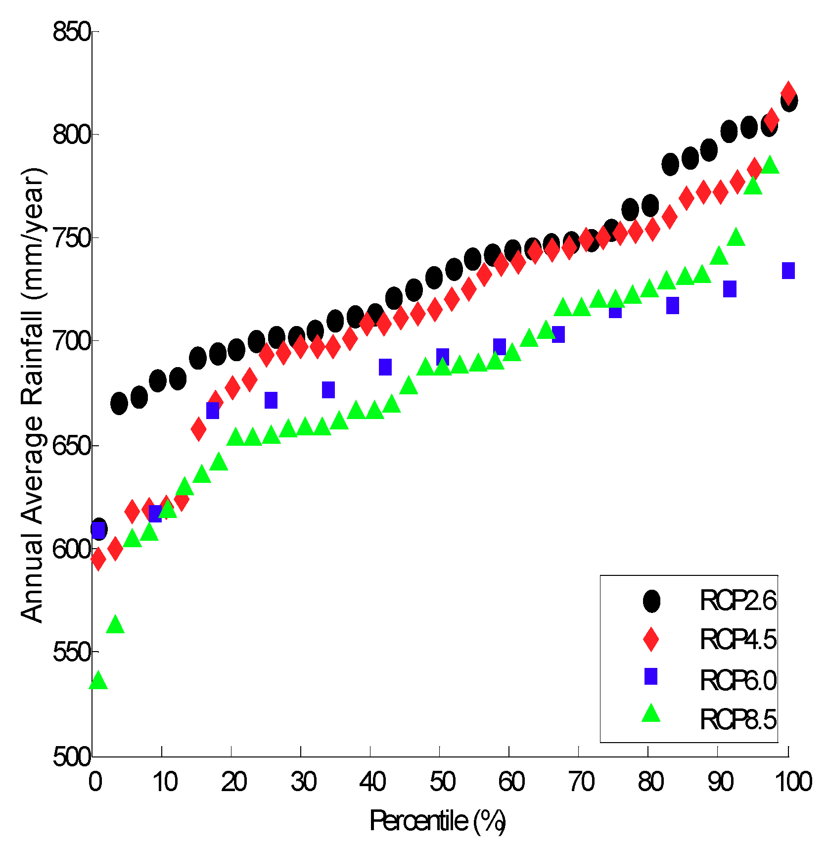
Since rainfall amounts are one of the most important inputs for crop growth, the annual average rainfall depth (mm/year) for each of the four RCPs and model outputs were calculated for the year 2050 to 2100 for a boarder location between Wilson and Atascosa counties (Figure 7). For this location (latitude 29.0625° longitude −98.3125°), the results show that, on average, precipitation regimes tend to decline from the Baseline scenario (RCP8.5) to high mitigation scenarios (RCP2.6), suggesting that climatic change can severely impact crops. For each RCP, the models at 25th, 50th, and 75th percentiles were selected to represent projected dry, median, and wet scenarios (

Table 1. Representative Concentration Pathways, models, institution, and modeling center.

RCP	Percentile	Model	Institution	Modeling Center
2.6	25	ipsl-cm5a-lr.1	Institut Pierre-Simon Laplace	IPSL
	50	canesm2.5	Canadian Centre for Climate Modelling and Analysis	CCCMA
	75	csiro-mk3-6-0.3	Commonwealth Scientific and Industrial Research Organization in collaboration with Queensland Climate Change Centre of Excellence	CSIRO-QCCCE
4.5	25	mpi-esm-lr.1	Max-Planck-Institut für Meteorologie (Max Planck Institute for Meteorology)	MPI-M
	50	gfdl-esm2m.1	NOAA Geophysical Fluid Dynamics Laboratory	NOAA-GFDL
	75	mri-cgcm3.1	Meteorological Research Institute	MRI
6.0	25	gfdl-esm2m.1	NOAA Geophysical Fluid Dynamics Laboratory	NOAA-GFDL
	50	ccsm4.1	National Center for Atmospheric Research	NCAR
	75	noresm1-m.1	Norwegian Climate Centre	NCC
8.5	25	miroc5.1	Atmosphere and Ocean Research Institute (The University of Tokyo), National Institute for Environmental Studies, and Japan Agency for Marine-Earth Science and Technology	MIROC
	50	miroc5.2	Atmosphere and Ocean Research Institute (The University of Tokyo), National Institute for Environmental Studies, and Japan Agency for Marine-Earth Science and Technology	MIROC
	75	ccsm4.1	National Center for Atmospheric Research	NCAR

).

4.4. ALMANAC Yield Maps

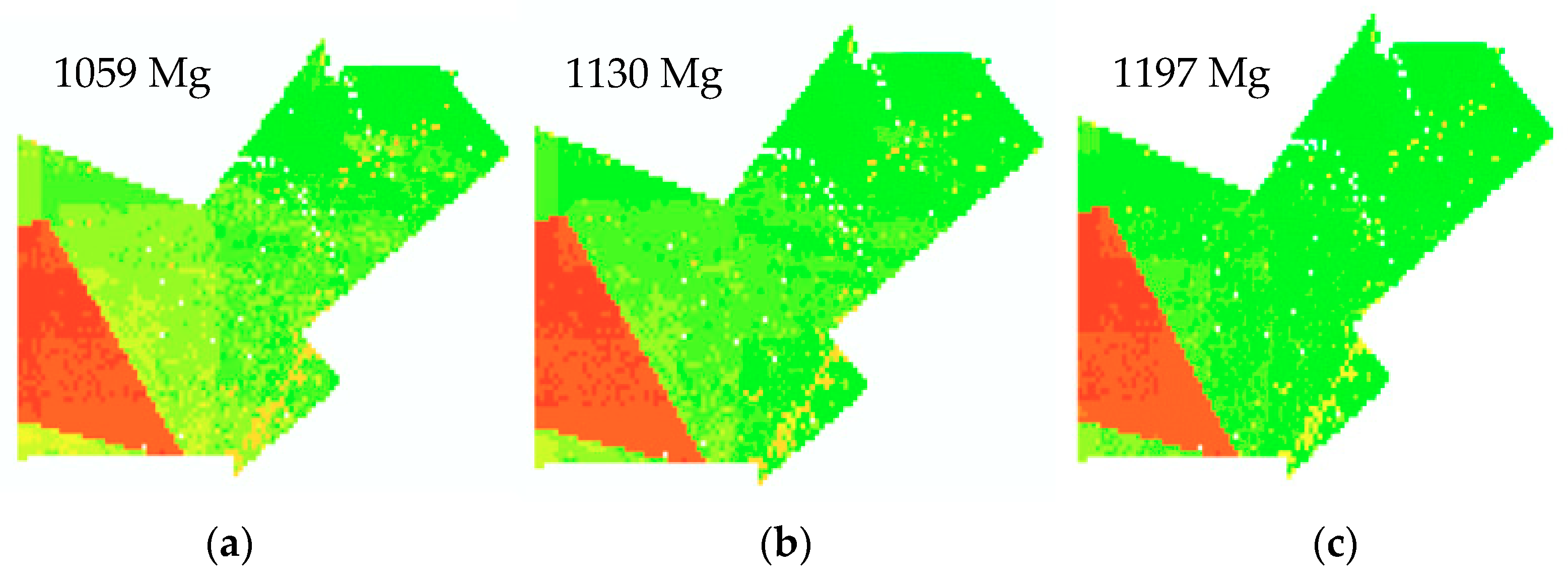
The climate data obtained from the scenarios presented in Table 1 were converted into ALMANAC compatible weather files and were used as precipitation and temperature (minimum and maximum daily temperature) inputs to obtain yield maps (Figure 8 and Figure 9 illustrate these maps for selected scenarios). Batch files were used in ALMANAC where each coordinate within the spatial domain of interest was executed, all while ensuring that each weather station was feeding data to its respective coordinate. This was accomplished with the help of ArcMap GIS, so that each coordinate would draw data from the closest weather station. In order to better determine the effect of percentile on the yield, the three percentiles of scenario 2.6 were mapped, as shown in Figure 9.

The RCP 2.6 maps with the three different percentiles show an expected trend: the 25th percentile considers less rainfall, the 75th percentile considers more rainfall, and with the 50th falling directly in the middle of the two. Higher biomass yield is observed with more rainfall. In order to ensure that the yield obtained from each future weather scenario is significantly different from the historical, a paired t-test is executed with a confidence level of 90% percent. The results of the paired t-test conclude that, except for RCP 2.6 25th, all future weather scenarios significantly differ from the historical scenario (1950–2000).

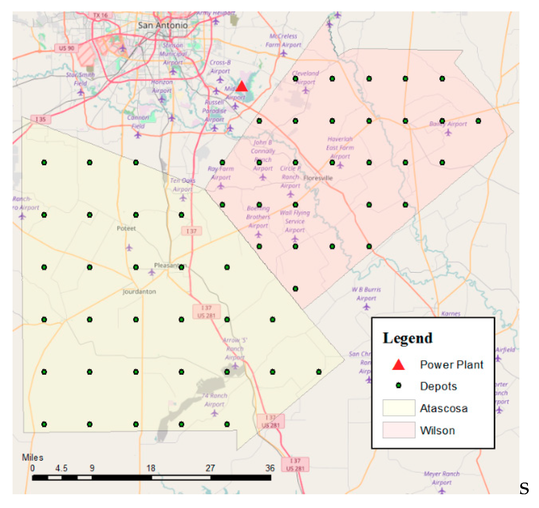
4.5. Depot Selection

In order to create a realistic supply chain design, a heuristic is introduced to define the set of potential depot locations. The proposed heuristic rounds the number of depots that are required by dividing the total demand between the depot capacities. Furthermore, the ratio of 1:10 is utilized to calculate the number of potential locations for the counties. The locations are distributed evenly to define a uniform arrangement that covers the whole county area. Thirty potential depot locations are considered over each county (Figure 10), with each depot having a total capacity of 300,000 Mg of switchgrass ($u_j$).

The cost of one depot is $333,000 (${\xi }_j$) [26]; this cost is annualized for the historical scenario using expression (10).

$$\mathrm{EAC}=\frac{\mathrm{r}\left(\mathrm{NPV}\right)}{1-\frac{1}{{\left(1+\mathrm{r}\right)}^{\mathrm{t}}}}$$

(10)

where, NPV [$] stand for net present value (depot investment cost), $r$ [–] is the interest rate, and $t$ [year] is the expected lifetime of the project, and $EAC$ is the equivalent annual cost [$]. A 15-year investment at a 5% interest rate is assumed.

4.6. Costs

Calculating the cost of switchgrass for co-firing biomass may be broken into two parts: harvesting and transportation costs.

Harvesting costs are inclusive of rent, baling, fertilizing, and swathing [27]. The cost of rent per hectare varies by county. It is assumed that the land will not be irrigated when selecting rent prices. The cost figures shown in

Table 2. Switchgrass Production Costs.

Item	Unit	Cost
Rent Atascosa County (${\mathit{R}}_{\mathbf{1}}$)	hectare	$38.30
Rent Wilson County (${\mathit{R}}_{\mathbf{2}}$)	hectare	$53.13
Swathing ($\mathbf{\alpha }$)	hectare	$32.49
Baling ($\mathbf{\beta }$)	ton	$12.42
Fertilizing ($\mathbf{\gamma }$)	hectare	$10.23

and

Table 3. Transportation Costs.

Item	Unit	Value Used
Average Truck Speed ($\mathit{v}$)	Km/hr.	60
Round Trip Factor ($\mathbf{\theta }$)		2
Truck Operational Cost ($\mathbf{\omega }$)	Per hour	$48.40
Small Truck Load Capacity (${\mathbf{\rho }}^{{\mathit{T}}_{\mathbf{1}}}\mathbf{,}{\mathbf{\rho }}^{{\mathit{T}}_{\mathbf{3}}}$)	Metric ton	3.63
Large Truck Load Capacity (${\mathbf{\rho }}^{{\mathit{T}}_{\mathbf{2}}}$)	Metric ton	21.76
Loading Cost ($\mathit{L}$)	Per metric ton	$3.59
Unloading Cost ($\mathit{U}$)	Per metric ton	$3.58
Stacking Cost ($\mathbf{\mu }$)	Per metric ton	$0.44

are based on the Integrated Biomass Supply Analysis and Logistics (IBSAL) models [26,27].

The values from Table 2 are then used in Equation (11). The harvesting cost (${\phi }_i$) changes by county as the cost of rent differs depending on the parcel selected ($i$); the other farming parameters (i.e., swathing, bailing, and fertilizing) remain constant.

$${\phi }_i=\left[\beta +\frac{\gamma +\alpha +R_i}{s_i}\right]$$

(11)

Transportation costs are calculated using distances ($x_{ij},x_{jk},or{x}_{ik}$ depending on the arc selected). Two transportation modes were used, one using a small truck to transport biomass from the parcel to the depot and a larger truck to move the biomass from depot to the power plant.

$${\mathsf{\tau }}_{\mathrm{ij}}^{{\mathrm{T}}_1}=\left(\mathrm{L}+\mathrm{U}+\mathsf{\mu }\right)+\frac{\frac{{\mathrm{x}}_{\mathrm{ij}}}{\mathrm{v}}\left(\mathsf{\theta }\right)\left(\mathsf{\omega }\right)}{{\mathsf{\rho }}^{{\mathrm{T}}_1}}$$

(12)

$${\mathsf{\tau }}_{\mathrm{jk}}^{{\mathrm{T}}_2}=\left(\mathrm{L}+\mathrm{U}+\mathsf{\mu }\right)+\frac{\frac{{\mathrm{x}}_{\mathrm{jk}}}{\mathrm{v}}\left(\mathsf{\theta }\right)\left(\mathsf{\omega }\right)}{{\mathsf{\rho }}^{{\mathrm{T}}_2}}$$

(13)

$${\mathsf{\tau }}_{\mathrm{ik}}^{{\mathrm{T}}_3}=\left(\mathrm{L}+\mathrm{U}+\mathsf{\mu }\right)+\frac{\frac{{\mathrm{x}}_{\mathrm{ik}}}{\mathrm{v}}\left(\mathsf{\theta }\right)\left(\mathsf{\omega }\right)}{{\mathsf{\rho }}^{{\mathrm{T}}_3}}$$

(14)

where, ${\tau }_{ij}^{T_1}$ refers to the transportation cost of the arc in question. The total costs of purchasing one ton from a parcel and delivering it to the depot/coal power plant are:

$$c_{ij}^{T_1}={\phi }_i+{\tau }_{ij}^{T_1}$$

(15)

$$c_{ik}^{T_2}={\phi }_i+{\tau }_{ik}^{T_2}$$

(16)

$$c_{jk}^{T_3}={\tau }_{jk}^{T_3}$$

(17)

5. Numerical Analysis

This section presents the results of our numerical analysis. The algorithms that were used in this study were written in Julia [28] JuMP and GUROBI 7.5.1 was used to solve the mathematical model. ArcMap GIS is used to visualize the solutions. The experiments were executed using a personal computer with an Intel (R) Core (TH) i5-6300U central processor unit operating at a frequency of 2.40 GHz and 8 GB of random-access memory.

5.1. Numerical Results

As part of the numerical experimentation, thirteen scenarios were analyzed. Specifically, the historical (baseline) scenario (from 1950–1999) and twelve climate change scenarios (from 2050–2099) were solved and analyzed. The solution maps and statistics of the climate change scenarios are outlined in Section 5.2.

The optimal solution of the baseline scenario is depicted in

Table 4. Baseline Optimal Solution.

RCP	Parcels Used	Depots	Avg. Supply	Variable Cost ($)	Fixed Cost ($)	Total Cost ($)
Baseline	913	4	1049 Mg	35.67 M	0.12 M	35.80 M

and in Figure 11. The total costs were divided into variable and fixed costs. The annual variable cost is determined by the production cost of the switchgrass (i.e., land management, bailing, transportations, and loading costs). The fixed cost involves the annualized depot investment cost.

According to the U.S. Energy Information Administration, the average cost for purchasing and shipping coal from Wisconsin to Texas is 30.55 dollars per short ton [1]. The cost of purchasing 20% of coal that was replaced is $35.41 M [20]. Thus, the total cost of co-firing is competitive, with a percentage difference of a little over 1%. For instance, 1,214,483 Mg of CO₂ are reduced solely by replacing 20% of coal with switchgrass. It is estimated that the emissions from harvesting and transporting the switchgrass are 55,626 Mg of CO₂, thus, the effective decrease in emissions results in 1,158,867 Mg of CO₂. The emissions from the biomass cofiring supply chain are calculated using the arcs in the optimal solution and while considering the number of trips and distance traveled for each trip. The emission values that are assumed in this analysis are presented in

Table 5. Emission Values from Historical Supply Chain Design.

Activity	Emissions Produced	Unit	Reference
Bailing	2.6450	kg	IBSAL [29]
Loading	12.05	kg
Unloading	15.585	kg
Stacking	0.5850	kg
Total Harvest (Xij, Zik)	30.865	kg
Transport from Depot (Yjk)	28.22	kg
Small Truck Transport	0.3014	kg/km	EPA Climate Dealership [30]
Large Truck Transport	0.8886	kg/km

. The competitiveness of the biomass SC is stressed even more if the environmental and social cost of carbon (SCC) from the lowered GHG emissions is considered. For the baseline scenario, considering a SCC of $36/Mg per emissions reduced, resulting in savings of $41.72 M [17].

5.2. Sensitivity Analysis using Climate Change Scenarios

Climate change scenarios were created to determine climate effects on the supply chain design, as well as the average biomass supply. The analysis is focused on the network topology and the availability of biomass supply to assess the robustness of the baseline solution under climate change conditions. The parameters that were determined for each scenario are summarized in

Table 6. Climate Change Sensitivity Output.

RCP	%	Parcels Used	Depots	Avg. Supply
2.6	25	904	4	1059 Mg
	50	847	4	1130 Mg
	75	800	4	1197 Mg
4.5	25	801	3	1196 Mg
	50	855	4	1120 Mg
	75	758	4	1264 Mg
6.0	25	719	4	1124 Mg
	50	777	3	1233 Mg
	75	772	4	1241 Mg
8.5	25	824	5	1162 Mg
	50	830	3	1154 Mg
	75	725	4	1320 Mg

, along with the mapping of the illustrative solutions in Figure 12 and Figure 13.

Based on the results, the yield will be sufficient to meet the demand with a co-firing rate of 20% when considering climate variability in the region. Noteworthy, with higher average supply, less parcels are required to meet the demand, which leads to lower investment cost. Depot location changes based on the selected parcels; therefore, depending on climate variations depot might need to be relocated.

Over all the scenarios, the highest parcel count reached is 904. Regardless of the changing weather conditions in these scenarios, the demand for the 20% co-firing rate is always met. Moreover, there are still approximately 3200 parcels available in every scenario. Hence, if the demand (e.g., cofiring rate) increases, then there is still available area to meet the biomass demand.

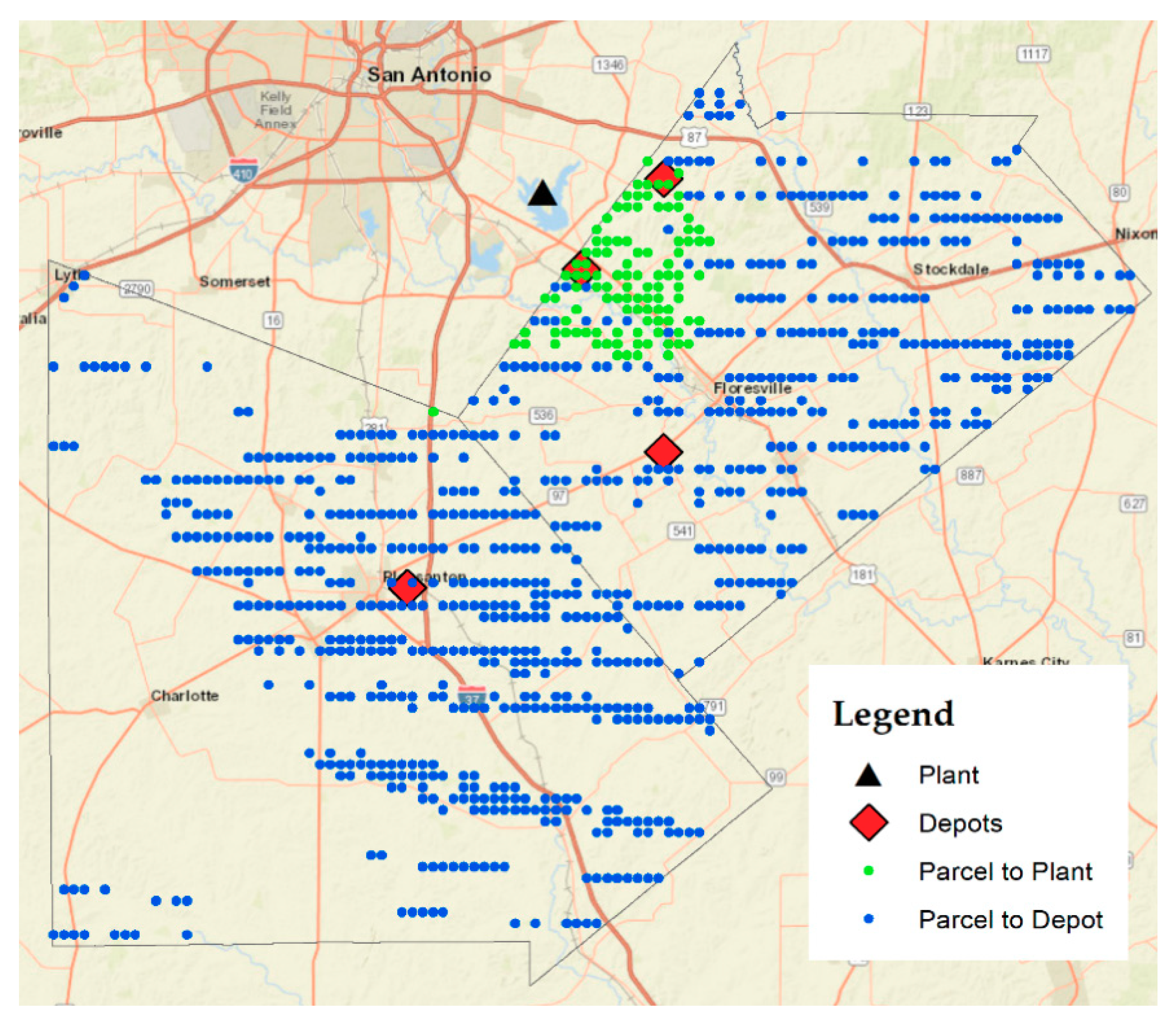
6. Conclusions and Future Work

In this paper, we presented a hybrid simulation-MILP optimization methodology for the design of a supply chain network for biomass cofiring in coal-fired power plants. Our model accounts for biomass supply (switchgrass yield) uncertainty through detailed ALMANAC simulations at the parcel level. Our model involves design and planning decisions of the supply chain to minimize the net cost, including investment in depots, harvesting, and transportation costs. This research fills a gap in the literature by developing a methodology that incorporated the analysis of the biomass supply at the parcel level and the impact of changing weather in the biomass availability. The proposed hybrid simulation-MILP optimization methodology is easily transferable to biofuel and biochemical supply chains. Moreover, the model can be adapted to incorporate various types of lignocellulosic biomass depending on the geographical region and the decision maker’s needs.

The resulting biomass logistics network for the baseline scenario (from 1950–2000) shows that the demand for a 20% co-firing rate target can be met by using 22% of the available parcels in the region. The overall annual investment cost of the supply chain shows to be competitive to coal. Even though, the overall cost resulted in being approximately 1% higher when compared to a coal supply scenario, when accounting for the decrease of the GHG emissions and the benefits to the communities in surrounding areas by the creation of new jobs, the slight difference in investment becomes justified. Future lines of research include: extending the model to a multi-criteria optimization model that minimizes costs, as well as land usage and emissions. Moreover, the model can be extended to a stochastic model that considers biomass supply variability and demand as random variables.