Smallholders’ Preferences for Improved Quinoa Varieties in the Peruvian Andes

Abstract
1. Introduction
2. Background
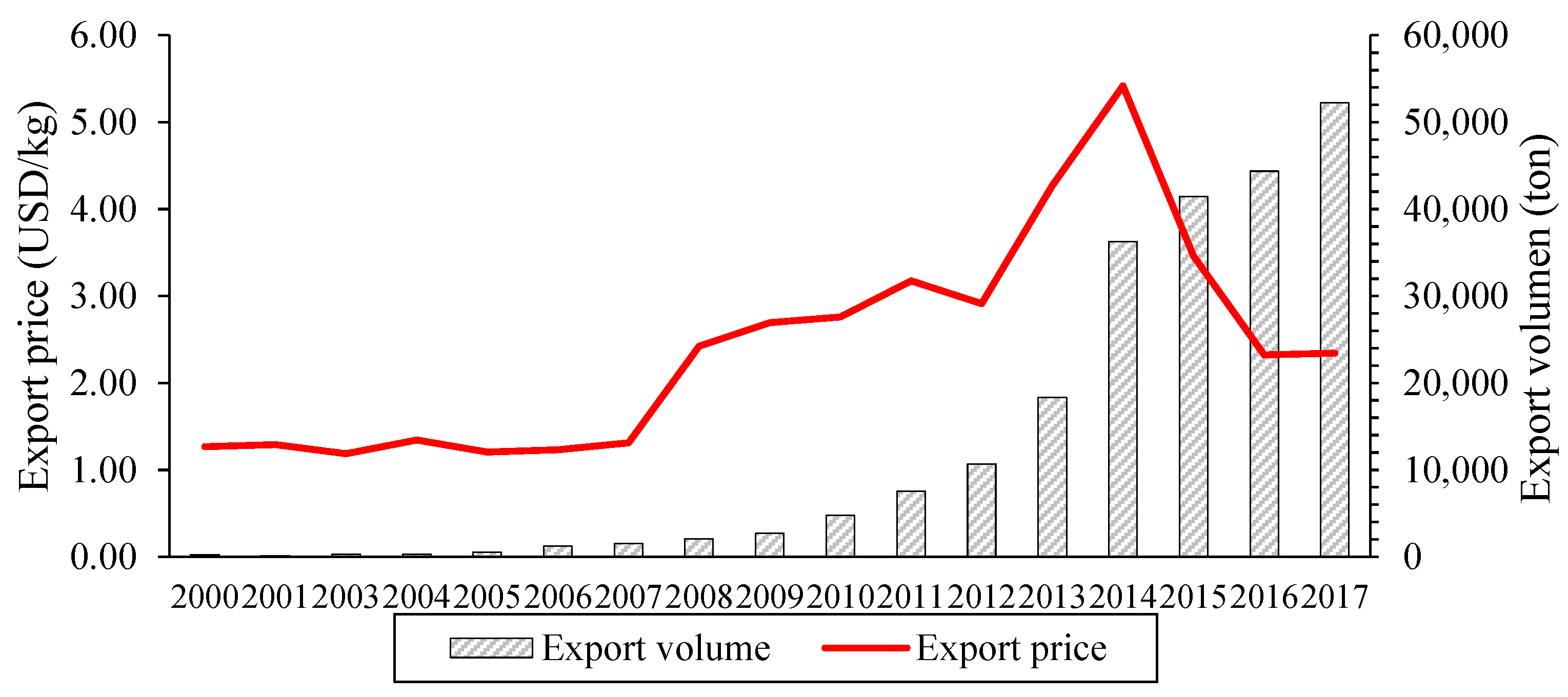
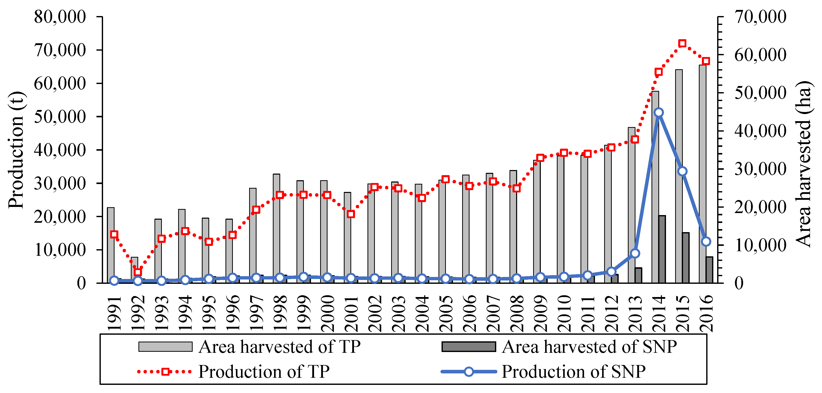
2.1. Export and Production of Quinoa
2.2. Development of Improved Quinoa Varieties
2.3. Quinoa and Food Security
3. Data and Methodology
3.1. Research Area
3.2. Choice Experiment
3.2.1. Concept
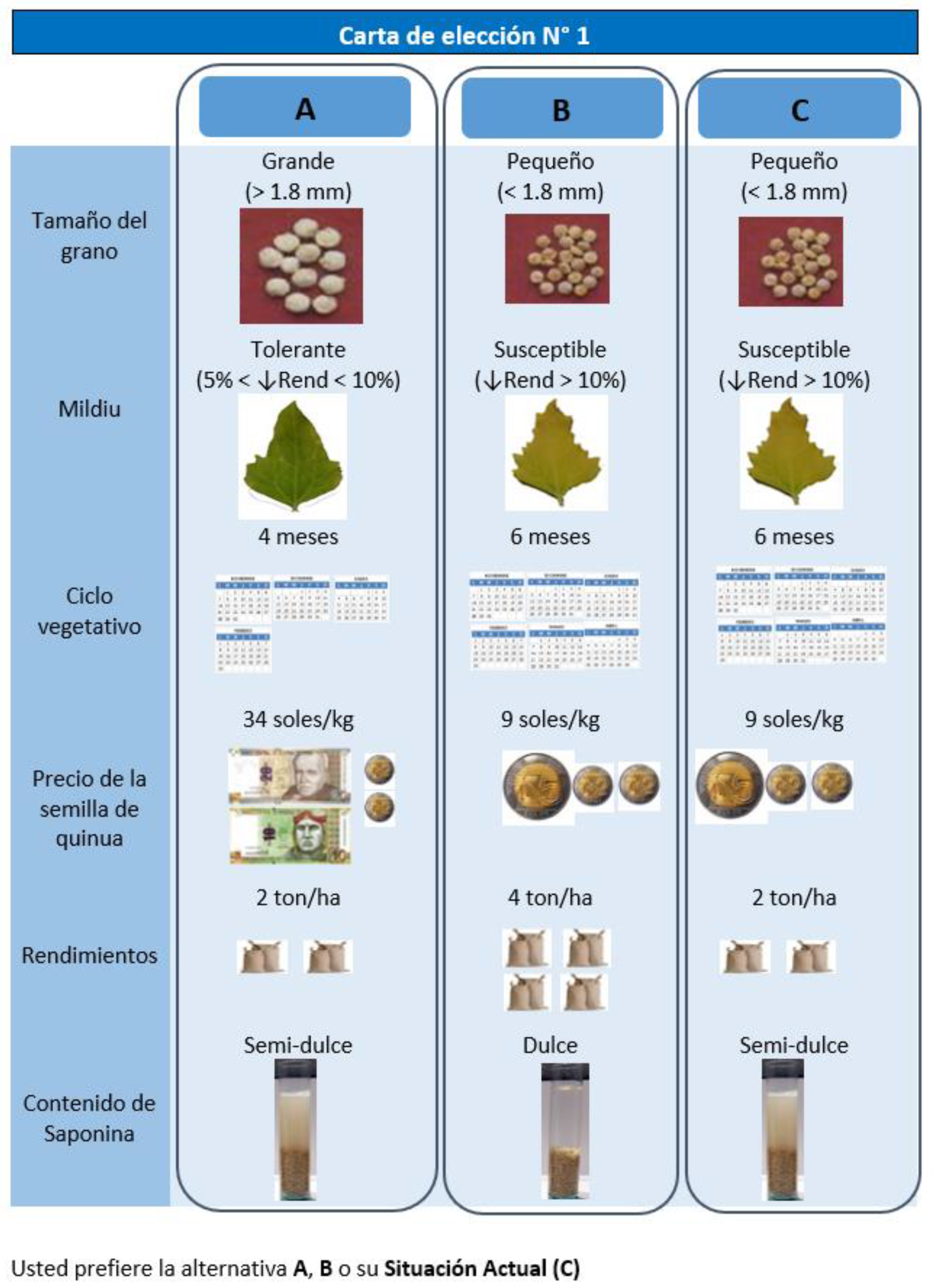
3.2.2. Design
3.2.3. Data Collection
3.2.4. Econometric Analysis
3.3. Measurement of Food Security
4. Results
4.1. Descriptive Statistics
4.2. GMNL Model Results
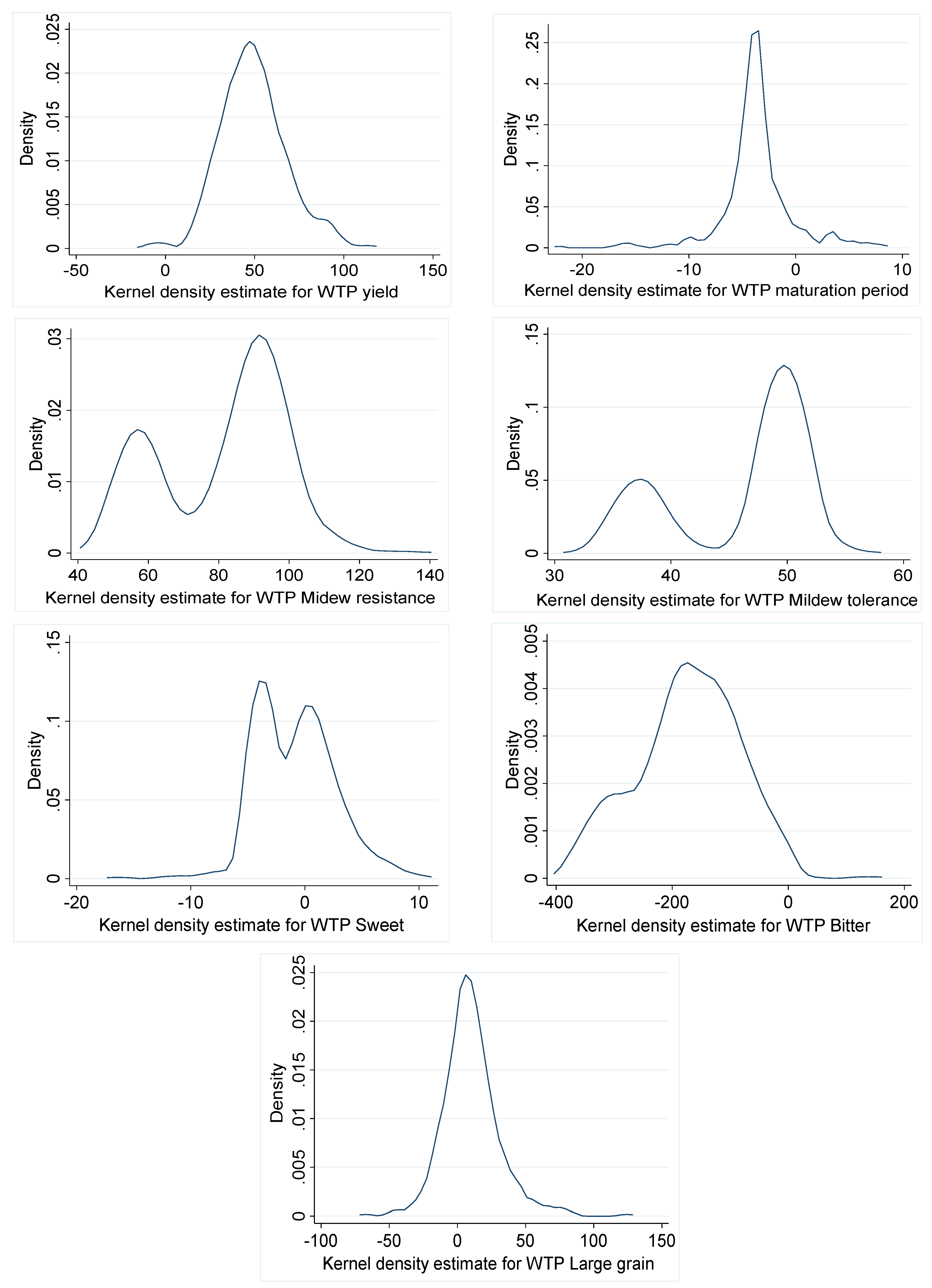
4.3. Willingness to Pay for Quinoa Traits
5. Discussion
6. Conclusions
Author Contributions
Funding
Acknowledgments
Conflicts of Interest
Appendix A

| Quinoa Varieties | Diameter (mm) | Color of Grain | Vegetative Cycle (days) | Saponin Content | Reaction to Mildew | Yield (ton/ha) | Experimental Stations in |
|---|---|---|---|---|---|---|---|
| Quillahuaman INIA | Large | White | 190–220 | Semi-sweet | Tolerance | 2.8 | Cusco |
| INIA 420—Negra collana | Small | Black | 140 | Sweet | Tolerance | 3.01 | Puno |
| INIA 415—Pasankalla | Large | Red | 144 | Sweet | Resistance | 3.5 | Puno |
| INIA 427—Amarilla Sacaca | Small-Large | Yellow orange | 160–180 | Bitter | Tolerance | 2.3 | Cusco |
| Salcedo INIA | Large | White | 150 | Sweet | Tolerance | 2.5 | Puno |
| ILLPA INIA | Large | White | 140 | Sweet | Tolerance | 3.1 | Puno |
| INIA 433—SANTA ANA/AIQ/FAO | Large | White | 160 | Bitter | Tolerance | 1.5–2 | Junín |
| INIA 431—Altiplano | Large | White | 150 | Sweet | Tolerance | 2.86 | Puno |
| 2010 | 2011 | 2012 | Average | ||||
|---|---|---|---|---|---|---|---|
| Mean | SD | Mean | SD | Mean | SD | ||
| N° farmers | 424 | 354 | 573 | ||||
| Area harvested (has) | 0.21 | 0.53 | 0.16 | 0.38 | 0.19 | 0.44 | 0.18 |
| Yield (kg/ha) | 1770 | 2250 | 1156 | 1066 | 1026 | 1736 | 1317 |
| Production (kg) | 228.91 | 763.98 | 163.56 | 489.56 | 234.51 | 1109.90 | 208.99 |
| % of sell (Sale/Production) | 0.18 | 0.30 | 0.17 | 0.30 | 0.15 | 0.29 | 0.16 |
| % of Self-consumption (Self-consumption/Production) | 0.56 | 0.31 | 0.60 | 0.33 | 0.60 | 0.34 | 0.59 |
| Price (soles/kg) | 3.71 | 1.02 | 3.74 | 0.84 | 4.12 | 1.10 | 3.86 |
| Consumption per capita | 19.98 | 41.93 | 15.02 | 18.72 | 15.70 | 22.33 | 16.90 |
| Consumption per adult equivalent | 31.63 | 71.48 | 20.65 | 24.94 | 21.40 | 27.74 | 24.56 |
| Choice Situation | Alternative | Grain Size | Mildew | Life Cycle (months) | Seed Price (PEN) | Yield (ton/ha) | Saponin Content |
|---|---|---|---|---|---|---|---|
| 1 | A | Large | Tolerance | 4 | 34 | 2 | Medium sweet |
| B | Small | Susceptible | 6 | 9 | 4 | Sweet | |
| 2 | A | Large | Resistance | 6 | 40 | 4 | Sweet |
| B | Small | Tolerance | 4 | 4 | 4 | Medium sweet | |
| 3 | A | Large | Susceptible | 5 | 24 | 1 | Sweet |
| B | Small | Tolerance | 5 | 14 | 1 | Bitter | |
| 4 | A | Small | Susceptible | 5 | 40 | 5 | Medium sweet |
| B | Large | Resistance | 5 | 4 | 2 | Sweet | |
| 5 | A | Small | Tolerance | 6 | 9 | 5 | Sweet |
| B | Large | Resistance | 4 | 34 | 3 | Medium sweet | |
| 6 | A | Small | Resistance | 4 | 4 | 3 | Medium sweet |
| B | Large | Tolerance | 6 | 40 | 6 | Bitter | |
| 7 | A | Large | Susceptible | 4 | 9 | 6 | Bitter |
| B | Small | Resistance | 6 | 34 | 3 | Medium sweet | |
| 8 | A | Large | Tolerance | 6 | 14 | 3 | Medium sweet |
| B | Small | Resistance | 4 | 24 | 6 | Bitter | |
| 9 | A | Small | Tolerance | 4 | 34 | 4 | Sweet |
| B | Large | Susceptible | 6 | 9 | 5 | Medium sweet | |
| 10 | A | Small | Resistance | 5 | 24 | 2 | Bitter |
| B | Large | Tolerance | 5 | 14 | 2 | Sweet | |
| 11 | A | Large | Resistance | 6 | 4 | 6 | Bitter |
| B | Small | Susceptible | 4 | 40 | 5 | Sweet | |
| 12 | A | Small | Susceptible | 5 | 14 | 1 | Bitter |
| B | Large | Susceptible | 5 | 24 | 1 | Bitter | |
| Status quo | C | Small | Susceptible | 6 | 9 | 2 | Medium sweet |
| Question Description | Yes | No | Percentage (N = 458) | ||||
|---|---|---|---|---|---|---|---|
| Often | Sometimes | Never | Refused | ||||
| Q2 | Worried whether food would run out | -- | -- | 3.71 | 47.82 | 46.51 | 1.97 |
| Q3 | Food that we bought just did not last | -- | -- | 1.75 | 34.72 | 61.79 | 1.75 |
| Q4 | Could not afford to eat balanced meals | -- | -- | 1.09 | 22.93 | 75.11 | 0.87 |
| Q5 | Relied on only a few kinds of low-cost food to feed children | -- | -- | 0.66 | 13.54 | 84.93 | 0.87 |
| Q6 | Could not feed the children a balanced meal | -- | -- | 0.44 | 10.04 | 88.65 | 0.87 |
| Q7 | Children were not eating enough | -- | -- | 0.22 | 6.33 | 92.58 | 0.87 |
| Q8 | Adult cut the size of meals or skipped them | 14.41 | 85.59 | 0.44 | 12.45 | 85.59 | 1.53 |
| Q9 | Eat less than felt should | 16.38 | 83.62 | -- | -- | -- | -- |
| Q10 | Hungry but did not eat | 12.88 | 87.12 | -- | -- | -- | -- |
| Q11 | Lose weight | 12.45 | 87.55 | -- | -- | -- | -- |
| Q12 | Adult did not eat for a whole day | 6.77 | 93.23 | 0.22 | 5.02 | 93.23 | 1.53 |
| Q13 | Cut the size of children’s meals | 5.02 | 94.98 | -- | -- | -- | -- |
| Q14 | Children ever skip meals | 3.28 | 96.72 | 0.00 | 2.40 | 96.72 | 0.87 |
| Q15 | Children ever hungry | 2.40 | 97.60 | -- | -- | -- | -- |
| Q16 | Children did not eat for a whole day | 2.18 | 97.82 | -- | -- | -- | -- |
| Full GMNL | GMNL-II | GMNL-I | |||||||
|---|---|---|---|---|---|---|---|---|---|
| Mean | SE | Mean | SE | Mean | SE | ||||
| Parameters | |||||||||
| ASC | −0.69 | 0.10 | *** | −0.71 | 0.11 | *** | −0.71 | 0.10 | *** |
| Seed price | −0.02 | 0.00 | *** | −0.02 | 0.00 | *** | −0.02 | 0.00 | *** |
| Yield | 0.88 | 0.06 | *** | 0.84 | 0.05 | *** | 0.76 | 0.04 | *** |
| Maturation period | −0.07 | 0.03 | *** | −0.06 | 0.03 | ** | −0.05 | 0.02 | * |
| Large grain | 0.16 | 0.06 | *** | 0.15 | 0.06 | *** | 0.12 | 0.05 | ** |
| Resistance | 1.40 | 0.10 | *** | 1.38 | 0.10 | *** | 1.23 | 0.07 | *** |
| Tolerance | 0.83 | 0.07 | *** | 0.80 | 0.07 | *** | 0.72 | 0.06 | *** |
| Bitter | −3.08 | 0.22 | *** | −2.96 | 0.17 | *** | −2.64 | 0.14 | *** |
| Sweet | −0.03 | 0.04 | −0.03 | 0.05 | −0.01 | 0.04 | |||
| Standard Deviations | |||||||||
| ASC | 1.22 | 0.12 | *** | 1.23 | 0.10 | *** | 1.19 | 0.10 | *** |
| Yield | 0.39 | 0.04 | *** | 0.39 | 0.04 | *** | 0.36 | 0.03 | *** |
| Maturation period | −0.14 | 0.05 | *** | −0.15 | 0.07 | ** | −0.19 | 0.04 | *** |
| Large grain | 0.55 | 0.11 | *** | 0.41 | 0.10 | *** | 0.52 | 0.08 | *** |
| Resistance | −0.21 | 0.16 | −0.29 | 0.11 | *** | 0.19 | 0.28 | ||
| Tolerance | 0.06 | 0.08 | 0.11 | 0.10 | 0.19 | 0.12 | |||
| Bitter | 1.82 | 0.19 | *** | 1.75 | 0.15 | *** | 1.49 | 0.11 | *** |
| Sweet | 0.07 | 0.11 | 0.01 | 0.23 | −0.08 | 0.09 | |||
| Tau | 0.60 | 0.09 | *** | 0.57 | 0.08 | *** | 0.35 | 0.08 | *** |
| Gamma | 0.24 | 0.18 | 0.00 | (FIXED) | 1.00 | (FIXED) | |||
| Observations | 16,488 | 16,488 | 16,488 | ||||||
| Chi squared | 343.11 | 465.41 | 817.56 | ||||||
| p-value | 0.00 | 0.00 | 0.00 | ||||||
| Log likelihood | −4452.19 | −4444.82 | −4464.48 | ||||||
| AIC | 8942.378 | 8925.647 | 8964.966 | ||||||
| BIC | 9088.875 | 9064.434 | 9103.753 | ||||||


References
- Hellin, J.; Higman, S. Crop Diversity and Livelihood Security in the Andes. Dev. Pract. 2005, 15, 165–174. [Google Scholar] [CrossRef]
- Jacobsen, S.E.; Mujica, A.; Ortiz, R. The Global Potential for Quinoa and Other Andean Crops. Food Rev. Int. 2003, 19, 139–148. [Google Scholar] [CrossRef]
- Padulosi, S.; Amaya, K.; Jäger, M.; Gotor, E.; Rojas, W.; Valdivia, R. A Holistic Approach to Enhance the Use of Neglected and Underutilized Species: The Case of Andean Grains in Bolivia and Peru. Sustainability 2014, 6, 1283–1312. [Google Scholar] [CrossRef]
- Ruiz, K.B.; Biondi, S.; Oses, R.; Acuña-Rodríguez, I.S.; Antognoni, F.; Martinez-Mosqueira, E.A.; Coulibaly, A.; Canahua-Murillo, A.; Pinto, M.; Zurita-Silva, A.; et al. Quinoa Biodiversity and Sustainability for Food Security under Climate Change. A Review. Agron. Sustain. Dev. 2014, 34, 349–359. [Google Scholar] [CrossRef]
- Lester, G.E. Organic versus Conventionally Grown Produce: Quality Differences, and Guidelines for Comparison Studies. HortScience 2006, 41, 296–300. [Google Scholar]
- Ofstehage, A. The Construction of an Alternative Quinoa Economy: Balancing Solidarity, Household Needs, and Profit in San Agustín, Bolivia. Agric. Hum. Values 2012, 29, 441–454. [Google Scholar] [CrossRef]
- Bazile, D.; Bertero, D.; Nieto, C. State of the Art Report on Quinoa around the World in 2013; FAO: Rome, Italy, 2015. [Google Scholar]
- Bazile, D.; Pulvento, C.; Verniau, A.; Al-Nusairi, M.S.; Ba, D.; Breidy, J.; Hassan, L.; Mohammed, M.I.; Mambetov, O.; Otambekova, M.; et al. Worldwide Evaluations of Quinoa: Preliminary Results from Post International Year of Quinoa FAO Projects in Nine Countries. Front. Plant Sci. 2016, 7, 850. [Google Scholar] [CrossRef] [PubMed]
- Zurita-Silva, A.; Fuentes, F.; Zamora, P.; Jacobsen, S.E.; Schwember, A.R. Breeding Quinoa (Chenopodium Quinoa Willd.): Potential and Perspectives. Mol. Breed. 2014, 34, 13–30. [Google Scholar] [CrossRef]
- Nowak, V.; Du, J.; Charrondière, U.R. Assessment of the Nutritional Composition of Quinoa (Chenopodium Quinoa Willd.). Food Chem. 2016, 193, 47–54. [Google Scholar] [CrossRef] [PubMed]
- Escuredo, O.; González Martín, M.I.; Wells Moncada, G.; Fischer, S.; Hernández Hierro, J.M. Amino Acid Profile of the Quinoa (Chenopodium quinoa Willd.) Using near Infrared Spectroscopy and Chemometric Techniques. J. Cereal Sci. 2014, 60, 67–74. [Google Scholar] [CrossRef]
- Elgeti, D.; Nordlohne, S.D.; Föste, M.; Besl, M.; Linden, M.H.; Heinz, V.; Jekle, M.; Becker, T. Volume and Texture Improvement of Gluten-Free Bread Using Quinoa White Flour. J. Cereal Sci. 2014, 59, 41–47. [Google Scholar] [CrossRef]
- Alvarez-Jubete, L.; Arendt, E.K.; Gallagher, E. Nutritive Value of Pseudocereals and Their Increasing Use as Functional Gluten-Free Ingredients. Trends Food Sci. Technol. 2010, 21, 106–113. [Google Scholar] [CrossRef]
- Simnadis, T.G.; Tapsell, L.C.; Beck, E.J. Physiological Effects Associated with Quinoa Consumption and Implications for Research Involving Humans: A Review. Plant Foods Hum. Nutr. 2015, 70, 238–249. [Google Scholar] [CrossRef] [PubMed]
- Jacobsen, S.-E. The Worldwide Potential for Quinoa (Chenopodium quinoa Willd.). Food Rev. Int. 2003, 19, 167–177. [Google Scholar] [CrossRef]
- Danielsen, S.; Munk, L. Evaluation of Disease Assessment Methods in Quinoa for Their Ability to Predict Yield Loss Caused by Downy Mildew. Crop Prot. 2004, 23, 219–228. [Google Scholar] [CrossRef]
- Sibiya, J.; Tongoona, P.; Derera, J.; Makandaa, I. Farmers’ Desired Traits and Selection Criteria for Maize Varieties and Their Implications for Maize Breeding: A Case Study from Kwazulu-Natal Province, South Africa. J. Agric. Rural Dev. Trop. Subtrop. 2013, 114, 39–49. [Google Scholar]
- Kassie, G.T.; Abdulai, A.; Greene, W.H.; Shiferaw, B.; Abate, T.; Tarekegne, A.; Sutcliffe, C. Modeling Preference and Willingness to Pay for Drought Tolerance (DT) in Maize in Rural Zimbabwe. World Dev. 2017, 94, 465–477. [Google Scholar] [CrossRef] [PubMed]
- Sánchez-Toledano, B.I.; Kallas, Z.; Gil-Roig, J.M. Farmer Preference for Improved Corn Seeds in Chiapas, Mexico: A Choice Experiment Approach. Span. J. Agric. Res. 2017, 15, e0116. [Google Scholar] [CrossRef]
- Smale, M.; Diressie, M.T.; Birol, E. Understanding the Potential for Adoption of High-Iron Varieties of Pearl Millet in Maharashtra, India: What Explains Their Popularity? Food Secur. 2016, 8, 331–344. [Google Scholar] [CrossRef]
- Lambrecht, I.; Vranken, L.; Merckx, R.; Vanlauwe, B.; Maertens, M. Ex Ante Appraisal of Agricultural Research and Extension: A Choice Experiment on Climbing Beans in Burundi. Outlook Agric. 2015, 44, 61–67. [Google Scholar] [CrossRef]
- Ward, P.S.; Ortega, D.L.; Spielman, D.J.; Singh, V. Heterogeneous Demand for Drought-Tolerant Rice: Evidence from Bihar, India. World Dev. 2014, 64, 125–139. [Google Scholar] [CrossRef]
- Asrat, S.; Yesuf, M.; Carlsson, F.; Wale, E. Farmers’ Preferences for Crop Variety Traits: Lessons for on-Farm Conservation and Technology Adoption. Ecol. Econ. 2010, 69, 2394–2401. [Google Scholar] [CrossRef]
- MINAGRI. Ministry of agriculture and Irrigation. Time Series of Agricultural Production. Available online: http://frenteweb.minagri.gob.pe/sisca/?mod=consulta_cult (accessed on 10 March 2018).
- Apaza, V.; Cáceres, G.; Estrada, R.; Pinedo, R. Catalogue of Commercial Varieties of Quinoa in Perú; FAO: Rome, Italy, 2015. [Google Scholar]
- Bedoya-Perales, N.S.; Pumi, G.; Mujica, A.; Talamini, E.; Padula, A.D. Quinoa Expansion in Peru and Its Implications for Land Use Management. Sustainability 2018, 10, 532. [Google Scholar] [CrossRef]
- Jacobsen, S.-E.; Mujica, A.; Jensen, C.R. The Resistance of Quinoa (Chenopodium quinoa Willd.) to Adverse Abiotic Factors. Food Rev. Int. 2003, 19, 99–109. [Google Scholar] [CrossRef]
- Bazile, D.; Jacobsen, S.-E.; Verniau, A. The Global Expansion of Quinoa: Trends and Limits. Front. Plant Sci. 2016, 7, 622. [Google Scholar] [CrossRef] [PubMed]
- Gomez-Pando, L.R.; Eguiluz-de la Barra, A. Developing Genetic Variability of Quinoa (Chenopodium quinoa Willd.) with Gamma Radiation for Use in Breeding Programs. Am. J. Plant Sci. 2013, 4, 349–355. [Google Scholar] [CrossRef]
- Mujica, A. Granos y Leguminosas Andinas. In Cultivos Marginados: Otra Perspectiva de 1492; Hernández Bermejo, J.E., León, J., Eds.; FAO: Rome, Italy, 1992; pp. 129–146. [Google Scholar]
- Bojanic, A. La Quinua: Cultivo Milenario Para Contribuir a La Seguridad Alimentaria Mundial; FAO: Rome, Italy, 2011. [Google Scholar]
- Repo-Carrasco, R.; Espinoza, C.; Jacobsen, S.-E. Nutritional Value and Use of the Andean Crops Quinoa (Chenopodium quinoa) and Kañiwa (Chenopodium pallidicaule). Food Rev. Int. 2003, 19, 179–189. [Google Scholar] [CrossRef]
- Jacobsen, S.E. The Situation for Quinoa and Its Production in Southern Bolivia: From Economic Success to Environmental Disaster. J. Agron. Crop Sci. 2011, 197, 390–399. [Google Scholar] [CrossRef]
- MIDIS. Mapa de Vulnerabilidad a La Inseguridad Alimentaria 2012; MIDIS: Lima, Perú, 2012. [Google Scholar]
- INEI. National Institute of Statistics and Informatics. National Survey of Strategic Programs (ENAPRES). Available online: http://iinei.inei.gob.pe/microdatos/ (accessed on 3 January 2018).
- DRAJ. Regional Direction of Agricultur of Junin. Time Series of Agricultural Production. Available online: http://www.agrojunin.gob.pe/?page_id=356 (accessed on 3 June 2018).
- Tapia, M.E.; Fries, A.M. Guía de Campo de Los Cultivos Andinos; FAO and ANPE: Lima, Perú, 2007.
- Rojas, W.; Pinto, M.; Alanoca, C.; Gómez Pando, L.; Leon-Lobos, P.; Alercia, A.; Diulgheroff, S.; Padulosi, S.; Bazile, D. Quinoa Genetic Resources and Ex Situ Conservation. In State of the Art Report on Quinoa around the World in 2013; FAO: Rome, Italy, 2015; pp. 56–82. [Google Scholar]
- Lancsar, E.; Fiebig, D.G.; Hole, A.R. Discrete Choice Experiments: A Guide to Model Specification, Estimation and Software. Pharmacoeconomics 2017, 35, 697–716. [Google Scholar] [CrossRef] [PubMed]
- Lancaster, K. A New Approach to Consumer Theory. Chic. J. 1966, 74, 132–157. [Google Scholar] [CrossRef]
- Louviere, J.J.; Flynn, T.N.; Carson, R.T. Discrete Choice Experiments Are Not Conjoint Analysis. J. Choice Model. 2010, 3, 57–72. [Google Scholar] [CrossRef]
- McFadden, D. Conditional Logit Analysis of Qualitative Choice Behavior. In Frontiers in Econometrics; Zarembka, P., Ed.; Academic Press: New York, NY, USA, 1973; pp. 105–142. [Google Scholar]
- Alfnes, F.; Guttormsen, A.G.; Steine, G.; Kolstad, K. Consumers’ Willingness to Pay for the Color of Salmon: A Choice Experiment with Real Economic Incentives. Am. J. Agric. Econ. 2006, 88, 1050–1061. [Google Scholar] [CrossRef]
- Loureiro, M.L.; Umberger, W.J. A Choice Experiment Model for Beef: What US Consumer Responses Tell Us about Relative Preferences for Food Safety, Country-of-Origin Labeling and Traceability. Food Policy 2007, 32, 496–514. [Google Scholar] [CrossRef]
- Ochieng, D.O.; Veettil, P.C.; Qaim, M. Farmers’ Preferences for Supermarket Contracts in Kenya. Food Policy 2017, 68, 100–111. [Google Scholar] [CrossRef]
- Van den Broeck, G.; Van Hoyweghen, K.; Maertens, M. Employment Conditions in the Senegalese Horticultural Export Industry: A Worker Perspective. Dev. Policy Rev. 2016, 34, 301–319. [Google Scholar] [CrossRef]
- Meemken, E.M.; Veettil, P.C.; Qaim, M. Toward Improving the Design of Sustainability Standards—A Gendered Analysis of Farmers’ Preferences. World Dev. 2017, 99, 285–298. [Google Scholar] [CrossRef]
- Ibnu, M.; Glasbergen, P.; Offermans, A.; Arifin, B. Farmer Preferences for Coffee Certification: A Conjoint Analysis of the Indonesian Smallholders. J. Agric. Sci. 2015, 7, 20–35. [Google Scholar] [CrossRef]
- Fiebig, D.G.; Keane, M.P.; Louviere, J.; Wasi, N. The Generalized Multinomial Logit Model: Accounting for Scale and Coefficient Heterogeneity. Mark. Sci. 2010, 29, 393–421. [Google Scholar] [CrossRef]
- Dalemans, F.; Muys, B.; Verwimp, A.; Van den Broeck, G.; Bohra, B.; Sharma, N.; Gowda, B.; Tollens, E.; Maertens, M. Redesigning Oilseed Tree Biofuel Systems in India. Energy Policy 2018, 115, 631–643. [Google Scholar] [CrossRef]
- Keane, M.; Wasi, N. Comparing Alternative Models of Heterogeneity in Consumer Choice Behavior. J. Appl. Econom. 2013, 28, 1018–1045. [Google Scholar] [CrossRef]
- Bickel, G.; Nord, M.; Price, C.; Hamilton, W.; Cook, J. Guide to Measuring Household Food Security Revised 2000; USDA: Washington, DC, USA, 2000.
- Lele, U.; Masters, W.A.; Kinabo, J.; Meenakshi, J.V.; Ramaswami, B.; Tagwireyi, J.; Goswami, S. Measuring Food and Nutrition Security: An Independent Technical Assessment and User’s Guide for Existing Indicators; FAO: Rome, Italy, 2016. [Google Scholar]
- Shiferaw, B.; Kassie, M.; Jaleta, M.; Yirga, C. Adoption of Improved Wheat Varieties and Impacts on Household Food Security in Ethiopia. Food Policy 2014, 44, 272–284. [Google Scholar] [CrossRef]
- Khonje, M.; Manda, J.; Alene, A.D.; Kassie, M. Analysis of Adoption and Impacts of Improved Maize Varieties in Eastern Zambia. World Dev. 2015, 66, 695–706. [Google Scholar] [CrossRef]


| Attribute | Levels | Dummy Coding |
|---|---|---|
| Seed price | 4 PEN/kg | Continuous variable |
| 9 PEN/kg (SQ) | ||
| 14 PEN/kg | ||
| 24 PEN/kg | ||
| 34 PEN/kg | ||
| 40 PEN/kg | ||
| Grain size | Small (SQ) | 0 |
| Large | 1 | |
| Susceptibility to mildew | Susceptible (SQ) | MD1 = 0; MD2 = 0 |
| Tolerance | MD1 = 0; MD2 = 1 | |
| Resistance | MD1 = 1; MD2 = 0 | |
| Maturation period | 4 months | Continuous variable |
| 5 months | ||
| 6 months (SQ) | ||
| Yield | 1 tons/ha | Continuous variable |
| 2 tons/ha (SQ) | ||
| 3 tons/ha | ||
| 4 tons/ha | ||
| 5 tons/ha | ||
| 6 tons/ha | ||
| Saponin content | High level (bitter) | SC1 = 1; SC2 = 0 |
| Low content (semi-sweet) (SQ) | SC1 = 0; SC2 = 0 | |
| Without saponin (sweet) | SC1 = 0; SC2 = 1 |
| Full Sample | Food Insecure Households | Food Secure Households | p-Value | |||||
|---|---|---|---|---|---|---|---|---|
| Mean | SD | Mean | SD | Mean | SD | |||
| Household head characteristics | ||||||||
| Age (year) | 50.42 | 13.25 | 49.71 | 12.79 | 50.72 | 13.45 | 0.454 | |
| Education level | ||||||||
| Primary education | 0.21 | 0.27 | 0.18 | 0.028 | *** | |||
| Secondary education | 0.49 | 0.47 | 0.50 | 0.529 | ||||
| Technical/university education | 0.22 | 0.14 | 0.25 | 0.007 | *** | |||
| Female head (dummy) | 0.13 | 0.11 | 0.14 | 0.354 | ||||
| Household characteristics | ||||||||
| Household size total | 3.74 | 1.52 | 4.03 | 1.50 | 3.62 | 1.51 | 0.008 | *** |
| Household size children | 1.09 | 1.20 | 1.33 | 1.27 | 0.98 | 1.16 | 0.005 | *** |
| Organization member (dummy) | 0.19 | 0.12 | 0.22 | 0.020 | ** | |||
| Net income 2014 | 20,435 | 45,242 | 8414 | 14,068 | 25,619 | 52,515 | 0.000 | *** |
| Net income per capita | 6442 | 14,236 | 2422 | 4385 | 8176 | 16,494 | 0.000 | *** |
| Net income per adult equivalent | 10,084 | 21,672 | 4042 | 7048 | 12,690 | 25,079 | 0.000 | *** |
| Poor household MPI 1 (dummy) | 0.07 | 0.15 | 0.03 | 0.000 | *** | |||
| Off-farm employment (dummy) | 0.11 | 0.05 | 0.00 | 0.13 | 0.00 | 0.008 | *** | |
| Farm characteristics | ||||||||
| Farm size (ha) | 4.65 | 6.04 | 2.56 | 2.57 | 5.56 | 6.84 | 0.000 | *** |
| Number of crops | 3.60 | 1.51 | 3.33 | 1.42 | 3.73 | 1.53 | 0.009 | ** |
| Number of tropical livestock units | 3.42 | 5.24 | 3.04 | 5.66 | 3.58 | 5.05 | 0.309 | |
| Quinoa area (ha) | 1.85 | 2.88 | 1.02 | 1.19 | 2.20 | 3.30 | 0.000 | *** |
| Specialization a | 0.43 | 0.24 | 0.44 | 0.24 | 0.42 | 0.24 | 0.387 | |
| Quinoa price (PEN/kg) | 6.86 | 2.20 | 6.49 | 2.45 | 7.02 | 2.07 | 0.026 | *** |
| Quinoa yield (kg/ha) | 2053 | 988 | 2126 | 1016 | 2022 | 975 | 0.305 | |
| Quinoa production (kg) | 4185 | 7884 | 2149 | 3178 | 5064 | 9063 | 0.000 | *** |
| Self-consumption (%) | 0.07 | 0.13 | 0.11 | 0.16 | 0.06 | 0.10 | 0.001 | *** |
| Seed-saving (%) | 0.03 | 0.05 | 0.04 | 0.06 | 0.03 | 0.05 | 0.182 | |
| Storage (%) | 0.13 | 0.27 | 0.11 | 0.24 | 0.14 | 0.28 | 0.198 | ** |
| Sell (%) | 0.76 | 0.31 | 0.75 | 0.30 | 0.76 | 0.31 | 0.620 | |
| Experience growing quinoa (year) | 10.51 | 11.09 | 8.29 | 8.79 | 11.43 | 11.80 | 0.007 | *** |
| Source of quinoa seeds | ||||||||
| from its last harvest (dummy) | 0.47 | 0.43 | 0.49 | 0.239 | ||||
| from other farmers (dummy) | 0.46 | 0.51 | 0.44 | 0.170 | ||||
| buying from INIA b (dummy) | 0.05 | 0.06 | 0.05 | 0.835 | ||||
| Use of Insecticide (dummy) | 0.69 | 0.76 | 0.66 | 0.037 | ** | |||
| Use of Fungicide (dummy) | 0.81 | 0.79 | 0.82 | 0.522 | ||||
| Mildew problem (dummy) | 0.82 | 0.78 | 0.84 | 0.164 | ||||
| Experience of frost | 0.40 | 0.40 | 0.41 | |||||
| Extension on quinoa (dummy) | 0.26 | 0.18 | 0.29 | 0.0116 | *** | |||
| Observations (number) | 458 | 138 | 320 | |||||
| Full Sample | Food Insecure Farmers | Food Secure Farmers | |||||||
|---|---|---|---|---|---|---|---|---|---|
| Mean | SE | Mean | SE | Mean | SE | ||||
| Parameters | |||||||||
| Seed price (PEN/kg) | −0.019 | 0.002 | *** | −0.027 | 0.009 | *** | -0.016 | 0.003 | *** |
| ASC | −0.724 | 0.109 | *** | −0.740 | 0.223 | *** | -0.741 | 0.138 | *** |
| Yield (ton) | 0.971 | 0.060 | *** | 0.991 | 0.224 | *** | 0.946 | 0.122 | *** |
| Maturation period (months) | −0.061 | 0.027 | ** | −0.076 | 0.058 | -0.063 | 0.032 | ** | |
| Large grain a | 0.184 | 0.060 | *** | 0.207 | 0.227 | 0.189 | 0.104 | * | |
| Resistance to Mildew b | 1.528 | 0.108 | *** | 1.565 | 0.325 | *** | 1.514 | 0.178 | *** |
| Tolerance to Mildew b | 0.903 | 0.078 | *** | 1.017 | 0.196 | *** | 0.814 | 0.103 | *** |
| Bitter c | −3.308 | 0.222 | *** | −3.493 | 0.909 | *** | -3.194 | 0.451 | *** |
| Sweet c | −0.027 | 0.048 | −0.106 | 0.098 | 0.012 | 0.058 | |||
| Standard Deviations | |||||||||
| ASC | 1.231 | 0.084 | *** | 1.145 | 0.205 | *** | 1.298 | 0.112 | *** |
| Yield | 0.465 | 0.047 | *** | 0.410 | 0.151 | *** | 0.409 | 0.050 | *** |
| Maturation period | −0.127 | 0.049 | ** | 0.276 | 0.120 | ** | -0.079 | 0.063 | |
| Large grain | 0.638 | 0.088 | *** | 0.773 | 0.422 | * | 0.608 | 0.150 | *** |
| Resistance to Mildew | 0.364 | 0.120 | *** | −0.359 | 0.816 | -0.363 | 0.165 | ** | |
| Tolerance to Mildew | −0.012 | 0.072 | 0.178 | 0.322 | -0.094 | 0.083 | |||
| Bitter | 2.095 | 0.196 | *** | 2.163 | 0.640 | *** | 1.952 | 0.290 | *** |
| Sweet | 0.129 | 0.082 | 0.064 | 0.366 | -0.173 | 0.142 | |||
| τ | 0.651 | 0.067 | *** | 0.730 | 0.284 | ** | 0.653 | 0.155 | *** |
| γ | −0.483 | 0.203 | ** | −0.022 | 0.353 | -0.393 | 0.246 | ||
| Observations | 16488 | 4968 | 11520 | ||||||
| Chi squared | 386.641 | 66.485 | 155.771 | ||||||
| p-value | 0.000 | 0.000 | 0.000 | ||||||
| Log likelihood | −4425.066 | −1317.405 | −3103.917 | ||||||
| BIC | 9034.629 | 2796.514 | 6385.519 | ||||||
| AIC | 8888.132 | 2672.809 | 6245.834 | ||||||
| Attribute Level | Total | Food Insecure Farmers | Food Secure Farmers | ||||
|---|---|---|---|---|---|---|---|
| Mean | SD | Mean | SD | Mean | SD | ||
| Yield | 49.39 | 18.49 | 35.52 | 9.60 | 55.36 | 18.19 | *** |
| Maturation period | −3.62 | 3.31 | −3.01 n.s. | 5.50 | −3.89 | 1.57 | |
| Large grain | 10.06 | 20.78 | 8.00 n.s. | 18.02 | 10.95 | 21.83 | |
| Resistance to Mildew | 81.34 | 17.81 | 57.47 | 5.06 | 91.64 | 9.52 | *** |
| Tolerance to Mildew | 46.02 | 5.90 | 37.37 | 1.72 | 49.76 | 1.48 | *** |
| Bitter | −172.73 | 87.69 | −126.18 | 59.25 | −192.81 | 90.36 | *** |
| Sweet | −0.84 | 3.44 | −3.98 n.s. | 0.50 | 0.52 n.s. | 3.27 | |
| Observations | 458 | 138 | 320 | ||||
© 2018 by the authors. Licensee MDPI, Basel, Switzerland. This article is an open access article distributed under the terms and conditions of the Creative Commons Attribution (CC BY) license (http://creativecommons.org/licenses/by/4.0/).
Share and Cite
Gamboa, C.; Van den Broeck, G.; Maertens, M. Smallholders’ Preferences for Improved Quinoa Varieties in the Peruvian Andes. Sustainability 2018, 10, 3735. https://doi.org/10.3390/su10103735
Gamboa C, Van den Broeck G, Maertens M. Smallholders’ Preferences for Improved Quinoa Varieties in the Peruvian Andes. Sustainability. 2018; 10(10):3735. https://doi.org/10.3390/su10103735
Chicago/Turabian StyleGamboa, Cindybell, Goedele Van den Broeck, and Miet Maertens. 2018. "Smallholders’ Preferences for Improved Quinoa Varieties in the Peruvian Andes" Sustainability 10, no. 10: 3735. https://doi.org/10.3390/su10103735
APA StyleGamboa, C., Van den Broeck, G., & Maertens, M. (2018). Smallholders’ Preferences for Improved Quinoa Varieties in the Peruvian Andes. Sustainability, 10(10), 3735. https://doi.org/10.3390/su10103735