Land Consolidation Design Based on an Evaluation of Ecological Sensitivity

Abstract

Land consolidation engineering inevitably interferes with terrestrial ecosystems, leading to natural capital loss. Therefore, conducting an ecological sensitivity evaluation of a project area before consolidation engineering is very important for reducing unnecessary human interference. Conservation of terrestrial ecosystems and the biodiversity therein to the greatest possible extent is urgently needed. This research analyzes the interference by human activities caused by land consolidation engineering in terrestrial ecosystems. GIS technology, ecological values, landscape pattern indexes, and an ecological risk evaluation were used to construct an ecological sensitivity evaluation index. The coefficient of variation method and a comprehensive sensitivity rating evaluation were used to calculate the weights and results. The project area was divided into sensitivity zones according to the results, and the results and suggestions are as follows: In the highly eco-sensitive zone, where bare rocks, gravel, and grass-covered areas compose the main landscape type, vegetation should be restored, and forests should be planted. In the medium eco-sensitivity zone, where irrigated paddy fields and arid land compose the main landscape type, land parcels should be merged, and agricultural infrastructure should be constructed or improved. In the low eco-sensitivity zone, where forests compose the main landscape type, roads should be closed, natural habitat should be restored, and buffer zones should be created. This study provides suggestions for future land management decisions.

1. Introduction

Global population growth, urbanization, changing consumption patterns, and climate change are expected to challenge the ability of terrestrial systems to satisfy the increasing demands for food, energy, and natural resources [1,2,3,4,5]. Land consolidation is considered an instrument or entry point for rural development [6,7] and an important means of improving food production capacity and reconciling land use conflicts [8,9,10]. Land consolidation is considered a planning instrument that adapts to dynamic circumstances. The objectives of land consolidation in many countries have progressively evolved to cover more complex and wider ranges of activities and include strategies such as promoting rural development, facilitating nonagricultural uses of rural land, optimizing the layout of urban and rural land use, and protecting the environment [11,12,13,14,15,16,17,18,19]. In China, land consolidation policies are designed mainly to mitigate farmland losses with the aim of both increasing farmland area and improving agricultural productivity [20,21].

Most land consolidation practices involve the amalgamation of small plots into large plots and promote the construction of irrigation, drainage, roadways, and forest conservation buffers [22]. Thus, land consolidation engineering inevitably interferes with terrestrial ecosystems, leading to natural capital loss; for instance, the removal of vegetation leads to reduced habitat and loss of ecological benefits. In conjunction with ecosystem service losses, the abovementioned impacts increase the sensitivity of the project area. Some environmental problems caused by land engineering are more sensitive [23], especially those that involve landscape ecological effects [24], the soil, the hydrological environment, climate, biodiversity, etc. [25,26,27].

Ecological sensitivity refers to the reactions with which ecosystems cope with human interference and natural changes in the environment. These reactions indicate the difficulty and potential to solve ecological problems in a region. An ecological sensitivity evaluation is essentially a clear identification of environmental problems compared with the natural environment background [28]. Areas with high ecological sensitivity are prone to the degradation of ecosystem function under natural and anthropogenic pressures. Moreover, these areas are essential to the sustainable development of agriculture, and the environment in these areas needs improvement [29,30].

In addition to social and economic benefit analyses (which are the basis for decision making associated with land consolidation), conducting an ecological sensitivity evaluation of a project area before land consolidation engineering projects are carried out is very important. Such an evaluation could minimize the disturbance caused by land consolidation engineering and provide a reference or supplement for scientific decision-making with respect to the implementation of land management activities. This paper mainly discusses the ecological and environmental effects of land consolidation activities while omitting the social, economic, and political factors associated with land consolidation.

Guanling County, a rocky area that has experienced some of the most severe desertification, lies within Guizhou Province in China. Guanling has suffered severe land and soil erosion; moreover, its ecosystem is vulnerable, as it has experienced reverse succession and degeneration due to interference by human activities. However, because there is little arable land and a large population in this region, land consolidation can be seen as a way to increase the amount of cultivated land for food supplies. Therefore, conducting ecological sensitivity evaluations in the project area before conducting land consolidation is very important, as ecological sustainability can guarantee sustainable social and economic benefits [31].

Land consolidation changes the land (landscape) type, so the value of ecosystem services provided by different landscape types also changes. Consolidation activities reduce or eliminate hedges and merge small plots into blocks, which alters the area, circumference, and shape of the land parcels in the project area, leading to changes in landscape patterns. These changes then affect the connectivity and energy flow between plots [32]. During consolidation engineering, the topsoil is removed and replaced, and arid land is consolidated into paddy fields, both of which are at risk of soil infiltration. During the process of eliminating hedges and reducing land exploitation, land consolidation will also inevitably disturb or even eradicate the vegetation community, which can lead to reverse succession [33]. Therefore, this paper attempts to characterize ecological sensitivity using three sets of indicators: ecological value, landscape pattern characteristics, and the degree of ecological risk. Thus, this paper may provide a supplement for the traditional planning method that focuses on economic and social benefits while ignoring ecological risks. Moreover, this paper also provides a case reference for the implementation of regional land consolidation projects.

2. Materials and Methods

2.1. Study Area

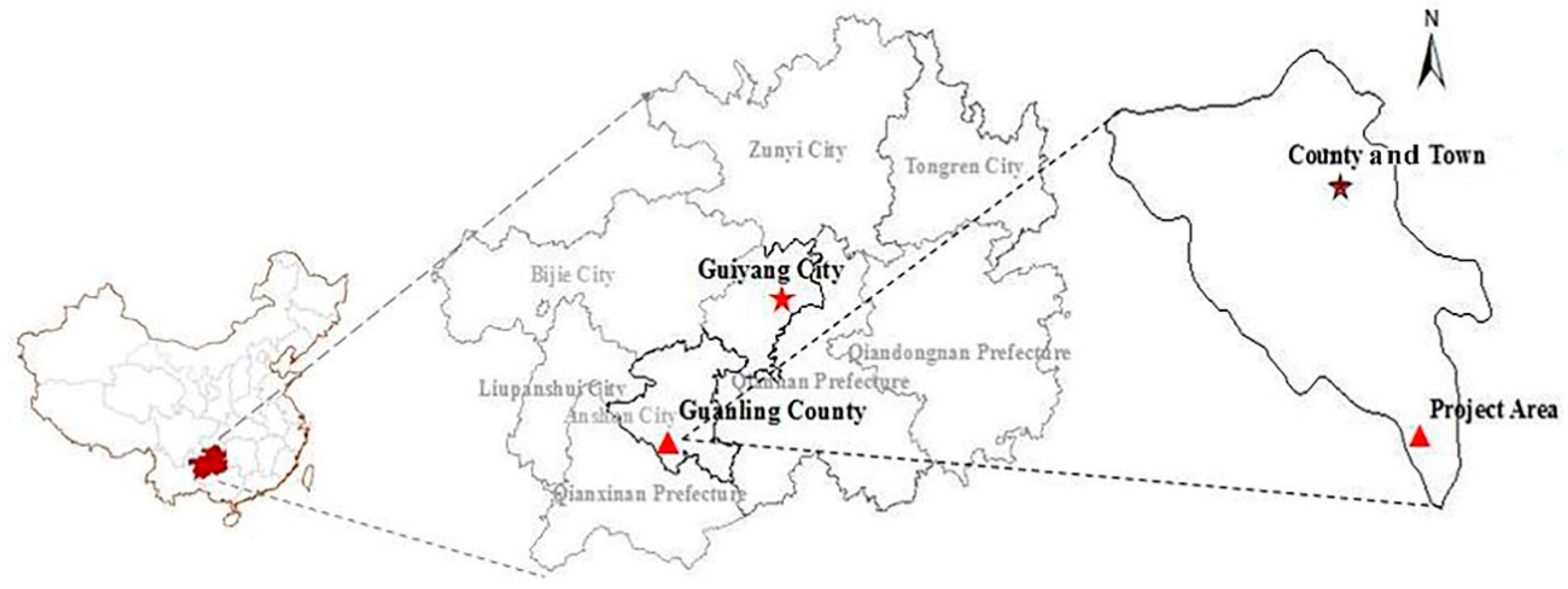
Guanling Autonomous County, which belongs to Anshun City in Guizhou Province, is located on the east coast of the Beipanjiang River (upstream of the Pearl River). Guanling has an area of 1470.49 km² and harbors 14 towns. Its elevation is high in the northwestern region and low in the southeastern region. The project area is located in Mugong Village in Guanling County (see Figure 1), which has a subtropical monsoon humid climate. Low mountains, clusters of peaks, and depressions are the main geomorphology types. The total project area is 32.37 hm², and the site has a longitudinal range of 105°41′47′′~105°2′21′′ E and a latitudinal range of 25°39′32′′~25°40′01′′ N. The annual average temperature is 17.9 centigrade, and the annual total temperature is 6542.9 centigrade. There is abundant rainfall suitable for crop growth during the hot season. The altitude ranges from 692.6 to 821.2 m a.s.l., and the topography is broken, with an uneven surface elevation, which is an obstacle to agriculture.

2.2. Data Sources

(1)

Map of land-use types: The data were derived from the database of the second land survey results of the country. The current land use map of Mugong Village in Guanling County has a scale of 1:2000 (provided by the Land Resource Bureau of Guanling County).

(2)

Vegetation cover data: The data were derived from 30 m Landsat Thematic Mapper (TM) images of the town of Bangui via the ArcGIS 10.2 (Environmental Systems Research Institute, Inc., Redlands, CA, USA; 2013) grid calculator tool combined with field investigations.

(3)

Ecological patch identification: The data were derived from field surveys. Several representative transects with different directions were selected in the project area along which to record visual measurements.

(4)

Soil type and texture: The soil profiles were established using field survey data. Soil samples were collected for analysis, and a 1:2000 soil type distribution map was created.

(5)

Grade: The data were derived from a Mugong village digital elevation model (DEM) map (provided by the Land Resources Bureau of Guanling County) via the slope extraction tool in ArcGIS 10.2.

(6)

Landscape pattern indexes: The landscape shape index, habitat connectivity index, maximum area of habitat patch index, and other landscape metrics were calculated with ArcGIS and FRAGSTATS 3.3 software (Department of Forest Science, Oregon State University, Corvallis, OR, USA).

(7)

Meteorological: The temperature and precipitation data were derived from the “Comprehensive agricultural regionalization of Guanling County” (provided by the Land Resources Bureau of Guanling County).

2.3. Research Methods

Ecological value is an important embodiment of the value evaluation of ecosystem service function [34]. The main purpose of ecological value assessments is to identify the important areas of various ecosystem services to filter key land parcels (patches) with ecological values for protection [35]. Ecological stress assessment focuses on the response of ecological processes to environmental changes and identifies high-risk factors and regions, whereas landscape connectivity evaluation takes the ecological system itself as the starting point to identify ecological land parcels that play an important role in maintaining the integrity of ecosystem structure. The evaluation of “importance–stress–connectivity” involves different key points to achieve ecosystem sustainability, ecosystem degradation prevention, and landscape integrity maintenance.

2.3.1. Evaluation Index

I. Ecological Value

Ecological value refers to the value of ecosystem services. Ecosystem services benefit humans directly or indirectly and are derived from an ecological system. These services include inputting useful materials and energy into economic and social systems, receiving and transforming waste from human society, and directly providing services to human beings. Ecological value is evaluated by the value of ecosystem services. Ouyang Zhiyun (1999) [36,37], Xie Gaodi (2003) [38], and others have quantified the value of ecosystem services. In a given region, the ecosystem provides different services for humankind, and the contributions of these services to quality of life vary. During the evaluation process, the ecosystem service value of various land use types is used as one of the evaluation indexes. In both a study by Xie Gaodi (2003) and a quantitative evaluation of ecosystem services in karst areas by Zhang Mingyang et al. (2009) [39], the ecosystem service value per unit area is taken as the calculation unit. The ecosystem service value = the area of land use type × the equivalent ecosystem service value for the land use type. The formula is as follows:

$$\mathrm{EV}={{\displaystyle \sum }}_{i=1}^n{p}_i\times v_i$$

(1)

In the formula, EV represents the value of ecosystem services, i is the land use type, p_i is the area of land use type i, and v_i is the ecosystem service value equivalent of land use type i. The ecosystem service value is a positive index in the evaluation. In the present study, vegetation coverage, flora diversity, and fauna diversity also affect ecological values in the project area. The greater the diversity of flora species is, the greater the density and the more likely an area is to act as a habitat patch. Therefore, these patches should be protected as habitat patches to minimize or avoid perturbations.

Vegetation structure type refers to the composition of vegetation in horizontal space and includes mainly the vegetation type distribution, area, and evolution tendency. Different vegetation types consist of different species and exhibit different species abundances. In the present study, scrub, sparse woodland, shrubs, grasses, and other secondary vegetation communities are the main vegetation communities in the project area. We should strategically avoid and prevent negative influences on community biodiversity and ecological sustainability following land consolidation engineering. Additionally, recommendations should be given for land use planning. Species richness is an indicator that measures the richness of species in a community; the larger the value is, the greater the richness of the species. This indicator is the simplest and most classic method to measure species diversity; the relative levels of importance of plant species in communities are represented in the form of numerical values. Jefferies (1997) [40] holds that the development of biodiversity is controlled mainly by the interaction of external environmental factors and internal factors. If the importance value of a plant species is high, the species adaptability is strong, and the quantity and density of that species in the community are also high. If the importance value of a plant species is low, that species has a weaker ability to adapt to the environment and to resist disturbance; thus, the species quantity and density in the community become low. The importance value of plant species is calculated as follows:

IV = [RDE + RDO + RFE] ÷ 3

(2)

in which IV is the importance value of a species, RDE is the relative density, RDO is the relative dominance, and RFE is the relative frequency.

The relative density is the density of an individual plant (species) in a quadrat divided by the individual density of all species in that quadrat. The density of a plant is the number of plants divided by the total area of the quadrat. Relative dominance is the projection coverage of an individual plant in a quadrat divided by the projection coverage of all the individuals in the quadrat. The projection coverage of plants = [(D1 + D2) ÷ 4]2 × 3.14 (D represents the north-south and east-west diameters of the crown of a plant). The relative frequency is the frequency of a plant divided by the total frequency of all the plants, and the frequency of a plant is the number of plants across all quadrats divided by the total number of quadrats [41].

II. Landscape Pattern Characteristics

The landscape pattern affects landscape function. Via land leveling and the merging of plots, land consolidation activities may affect the shape of patches, the area of the largest plot, and the connectivity between plots.

Landscape connectivity refers to the convenience or obstruction of a landscape to ecological flow and is an important index for measuring landscape ecological processes. Connectivity maintenance is one of the key factors protecting biodiversity and maintaining ecosystem stability and integrity. The probability of connectivity (PC) can not only reflect the connectivity of a landscape but also calculate the important value of parcel connectivity to a landscape, which is widely used in landscape planning. PC defines connectivity based on the possibility of direct diffusion between two habitat nodes and serves as the basis for assessing species migration intensity, frequency, or flexibility [35].

Therefore, patch shape, habitat connectivity, and the maximum area of habitat patches were selected as evaluation indexes [42,43,44,45,46,47].

(1) The landscape shape index (shape index) is the shape of a patch in a land-use type or within a whole landscape. This index measures patch shape complexity and is calculated by the degree of deviation between a patch shape and a circle or square. This index can be calculated in FRAGSTATS 3.3, and the formula is as follows:

SHAPE = Pij ÷ minPij

(3)

In the formula, Pij is the perimeter of a patch and is represented by the number of grid surfaces, and minPij is the minimum possible value of Pij. The shape index is unitless, and SHAPE ≥ 1. SHAPE = 1 indicates that the patches are maximally aggregated together (for example, similar to the shape of a square or rectangle), and the value of this index increases infinitely as the shape becomes increasingly irregular.

(2) LPI is the ratio of the largest patch to the total landscape area. This index is presented as a percentage, and the range is 0 < LPI ≤ 100. LPI is the ratio of the maximum size patch of one landscape type relative to the entire landscape area. The LPI value helps to determine the landscape model or dominance type of the landscape.

$$\mathrm{LPI}=\frac{\mathrm{M}}{\mathrm{A}}\times 100$$

(4)

In the formula above, M is the largest patch area in the landscape, and A is the total area of the landscape (m²).

(3) Habitat connectivity is used to measure the natural connectivity of relevant patch types [35] and to measure the proportion of certain patches in the landscape. The value of cohesion index increases as the proportion of the focal land type in the landscape increases. The patch cohesion index is sensitive to the degree of aggregation of the patch when the value of COHESION cohesion index is under the percolation threshold. The range is 0 ≤ cohesion index ≤ 100.

$$\mathrm{COHESION}=\left[1-\frac{{{\displaystyle \sum }}_{j=1}^n{p}_{ij}}{{{\displaystyle \sum }}_{j=1}^n{p}_{ij}\sqrt{a_{ij}}}\right]\times {\left[1-\frac{1}{\sqrt{A}}\right]}^{-1}\times 100$$

(5)

In the formula above, p_ij is the perimeter of a patch, a_ij is the area of the patch, and A is the total number of grids in the landscape. The patch cohesion index measures the natural connectivity of relevant patch types.

The landscape index describes the landscape pattern and its change characteristics, thus establishing the relationship between landscape patterns and landscape processes; the landscape index is the most commonly used method in landscape ecology research. As landscape pattern analysis software still depends on grid type data, the results obtained for the landscape index are influenced by the definition of the grain size when the data are converted [48,49]). As grain size increases in a landscape pattern, small patches will gradually merge into large patches, and some patches may disappear during the merging process. Consequently, the number of patches, border length, and the diversity of patches will decrease. Some scholars [46,50,51,52,53] believe that, with an increase in grain size, most landscape pattern index curves exhibit a significant inflection point or jump interval [54]. The first scale domain of landscape index changes with grain size can determine the size of grains in landscape pattern index analysis. On a relatively small scale, the first scale domain of the landscape index is concentrated mainly within the interval of 10 to 30 m, 20 to 30 m, or 10 to 40 m.

III. Ecological Risk Degree

Ecological risk degree indexes consider that land consolidation engineering might alter the microtopography, which would lead to soil erosion because of rainfall and relatively steeper slopes. The greater the slope value is, the more exposed the topsoil layer and the greater the risk of soil erosion will be given an equal amount of precipitation. The method for calculating soil erosion risk is as follows: rainfall × slope × grade of soil erosion risk of the land use type. The single-factor evaluation method was adopted from “Interim regulations on ecological functional zones of China (Ministry of Environmental Protection of PRC. September 1, 2002)”, “Technical guidelines to the demarcation of ecological protection red line (Ministry of Environmental Protection of PRC, [2015]56)” and “Classification criteria for soil erosion (SL190-2007)”. Related research on classification standards for ecological sensitivity index systems in ecological function zoning in China was taken as a reference [55,56,57]. The risk levels for different land-use types are classified as follows: Rocky desertification land is extremely sensitive to different types of soil erosion; farmland is highly sensitive to soil erosion; and grassy fields are moderately sensitive to soil erosion, followed by roads, woodlands, and built-up land. The calculation method for soil erosion risk is as follows:

Soil erosion risk = rainfall × slope sensitivity grade × grade of soil erosion risk of the land use type, that is:

$$\mathrm{WL}={\displaystyle \sum }_{i=1}^{n}J\times s_i\times LT{L}_i$$

(6)

In the above formula, WL is the soil erosion risk, i is the land use type in the project area, s_i is the average slope grade for land use type i, and LTL_i is the soil erosion risk grade for land use type i.

Soil texture is a very important factor in land consolidation. During land consolidation, some arid lands will be consolidated into paddy fields because of their soil characteristics and the demands of the farmer. Soil texture is closely related to crop growth and soil erosion. Therefore, the sensitivity of soil texture should also be analyzed as a factor in ecological sensitivity evaluations of land consolidation. Taking the research of Yang Guorong and others [58,59,60]; as a reference and considering land use characteristics in the project area, a single-factor evaluation method was adopted. The single factor was divided into five levels, namely, not sensitive, mildly sensitive, moderately sensitive, highly sensitive, and extremely sensitive, and these levels were given the values 1, 3, 5, 7, and 9, respectively [59]. The specific classification scheme is as follows (

Table 1. Single-factor sensitivity classification standard.

Indexes	Not Sensitive	Mildly Sensitive	Moderately Sensitive	Highly Sensitive	Extremely Sensitive
Rainfall (mm)	(0, 25)	(25, 100)	(100, 400)	(400, 600)	>600
Soil texture	Sand, stone	Clay, sandy soil	Loam, fine sandy soil	Loam, clay	Silt, sandy silt
Slope (°)	(0, 8)	(8, 15)	(15, 25)	(25, 35)	>35
Land use type	Herbs, marsh, water areas	Forests, grassland	Thin scrubland	Desert, arable land	Nonvegetated
Risk of soil erosion	Buildings	Forest, corridor	Grassland	Farmland	Rocky desert
Risk of water pollution	Forest	Grassland, sand and stone lands	Corridor	Farmland	Buildings

):

There are two sources of risk for water pollution in rural water systems: one is the discharge of domestic sewage from homesteads, and the other is nonpoint source pollution from agricultural chemical fertilizers. Therefore, the risk of water pollution is also considered an indicator of ecological risk. Buildings (including rural homesteads, domestic sewage, and human and livestock excrement discharge) pose the highest risk of water pollution of all land use types, followed by farmland (chemical fertilizer pollution), corridors (drainage on both sides of the road), barren grassland, and forests. The water pollution risk level is as follows: building > farmland > corridor > barren grassland > forest. The specific classification standard is presented in Table 1. The method for calculating water pollution risk is as follows:

$$\mathrm{WR}={{\displaystyle \sum }}_{i=1}^n{P}_i\times R_i$$

(7)

In the formula above, WR is the degree of water pollution risk, i is the land use type in the project area, P_i is the area of land use type i, and R_i is the water pollution risk level for land use type i. The ecological sensitivity evaluation indexes for land consolidation project areas are shown in

Table 2. Ecological sensitivity evaluation indexes for land consolidation.

Ecological Sensitivity Factors	Indexes	Calculation Method	Influence Direction
Ecological value	Value of ecosystem service	EV = ${\displaystyle \sum }_{i=1}^n{P}_i\times W_i$	+
	The habitat area of a species community	Plant species number and density	+
	Vegetation coverage	Vegetation coverage area/total project area	+
	Importance value of plant species in the community	IV = [RDE + RDO + RFE] ÷ 3	+
Landscape pattern characteristic	Landscape shape index	SHAPE = Pij ÷ minPij	+
	Habitat connectivity	COHESION	+
	The index of the largest patch in a landscape area	LPI = $\mathrm{m}/\mathrm{A}\times 100\%$	+
Degree of ecological risk	Degree of soil erosion risk	WL = ${\displaystyle \sum }_{i=1}^{n}J\times S_i\times LT{L}_i$	-
	Soil sensitivity	Soil sensitivity evaluation	-
	Water pollution risk level	WR = ${\displaystyle \sum }_{i=1}^n{P}_i\times R_i$	-

.

2.3.2. Weight Calculation Method

The coefficient of variation method was adopted for determining the weights of the evaluation factors [61,62]. The coefficient of variation is also known as the “standard differential”, which is another statistic that measures the degree of variability of the observed values with a data set. When the variation of two or more data are compared and when the measurement unit is the same as the average, the standard deviation can be directly compared. If the measurement units are not the same as those of the average, then the standard deviation cannot be used for a direct comparison; in this case, the ratio of the standard deviation and the average (relative value) should be compared. The calculation formula is as follow (Formula (8) and the calculation result is as

Table 3. The coefficient of variation method is used to determine the factor weight.

Factors	Ecological Value	Landscape Pattern Characteristic	Ecological Risk Degree
Mean value	2.73	3.65	3.16
Standard deviation	1.16	1.21	1.02
Coefficient of variation	0.42	0.34	0.35
Normalized weight	0.37	0.31	0.32

).

$$\mathrm{W}=\frac{v}{{{\displaystyle \sum }}_{i=1}^n{v}_i}=\frac{\raisebox{1ex}{$s$}\!\left/ \!\raisebox{-1ex}{$\overline{x}$}\right.}{{{\displaystyle \sum }}_{i=1}^n\left(s_i-\overline{x_i}\right)}$$

(8)

In the formula above, W is the weight of the evaluation factor, V is the coefficient of variation, S is the standard deviation, $\overline{x}$ is the average (mean value), and i is the number of factors.

2.3.3. Ecological Sensitivity Evaluation

The grid calculation tool of the ArcGIS spatial analyst module can be used for comprehensive multifactor evaluations of ecological sensitivity via the following equation:

$$\mathrm{SS}={{\displaystyle \sum }}_{i=1}^n{w}_i\left(a_1+a_2+\dots +a_i\right)$$

(9)

In the formula above, SS is the comprehensive ecological sensitivity index, which has a spatial unit of 30 m × 30 m; $W_i$ is the sensitivity weight of factor i, and $a_i$ is the grade classification of the sensitivity of factor i (i = 1, 2, … 10).

2.3.4. Ecological Sensitivity Classification

The ecological sensitivity level results were divided into 4 grades via natural breaks. Values of 6.1–8.0 indicate that a region is highly sensitive, values of 4.1–6.0 indicate moderate sensitivity, values of 2.1–4.0 indicate low sensitivity, and values of 1.0–2.0 indicate insensitivity.

3. Results Analysis

Stony desert is a unique desert type [63] that is characterized by a reduction or loss of ecosystem function. The project area is located in a typical rocky desertification mountainous area of Southwest China, where there is thin soil coverage and severe soil erosion. Zhang Mingyang’s [39] research on ecosystem classification and ecological parameter evaluation indexes in karst ecosystems served as a reference. The ecological parameters are described below.

3.1. Ecological Value Calculation

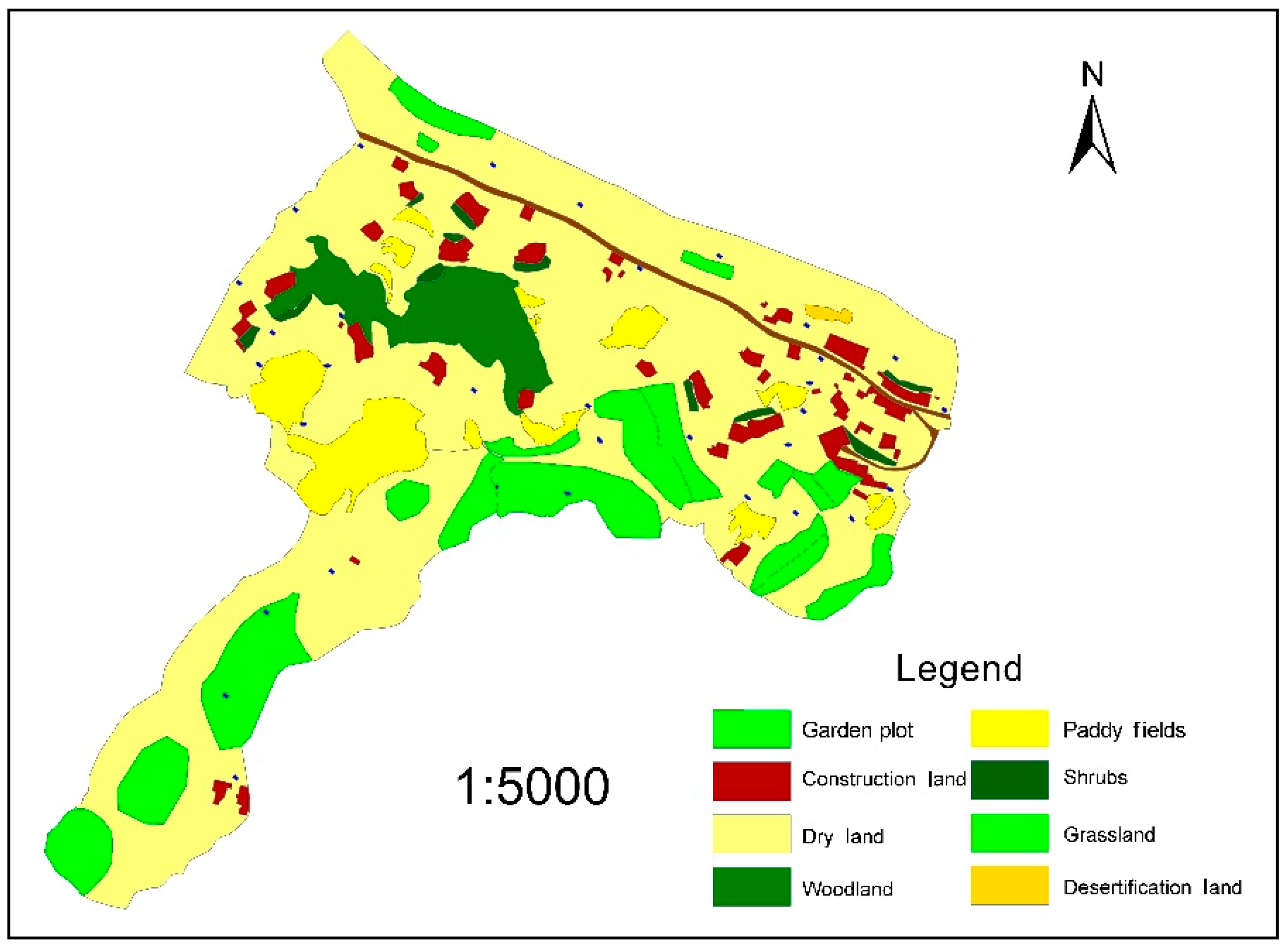
The landscape types in the project area include cultivated land (dry land and irrigated paddy fields), forests, corridors (field ridges, rural roads, land for irrigation and water conservation facilities), construction land (rural residential land and grave land), grassland, and rocky desert land (bare rock and gravel). Among these types, rocky desertification land includes mainly areas with high rock exposure rates (>70%) and low vegetation coverage (less than 5%). The land use types and their respective areas in the project region are shown in

Table 4. Landscape types and areas in the project region.

Landscape Type	Cultivated Land	Forests	Corridors	Construction Land	Grassland	Rocky Desertification Land
Area (hm2)	25.83	1.69	0.66	1.59	0.33	0.88
Proportion	79.82%	5.23%	2.05%	4.92%	1.03%	2.72%

(the data were obtained from project area mapping):

The total project area is 32.37 hm². Division of this area into a 30 m × 30 m grid resulted in 358 cells, which served as evaluation units. The results of Xie Gaodi [38] (

Table 5. Ecosystem service value per unit area of different terrestrial ecosystems in China (yuan/hm²).

Types of Ecosystem Services	Forest	Grassland	Cropland	Wetland	Water Body	Desert
Gas regulation	3097	707.9	442.4	1592.7	0	0
Climate regulation	2389.1	796.4	787.5	15,130.9	407	0
Water conservation	2831.5	707.9	530.9	13,715.2	18,033.2	26.5
Soil formation	3450.9	1725.5	1291.9	1513.1	8.8	17.7
Waste disposal	1159.2	1159.2	1451.2	16,086.6	16,086.6	8.8
Biodiversity	2884.6	964.5	628.2	2212.2	2203.3	300.8
Food production	88.5	265.5	884.9	265.5	88.5	8.8
Raw material	2300.6	44.2	88.5	61.9	8.8	0
Entertainment culture	1132.6	35.4	8.8	4910.9	3840.2	8.8

) and Zhang Mingyang [39] served as references for calculations of the values of ecosystem services in the evaluation units in the landscape via the area of each landscape type and its ecosystem service value.

Cultivated land comprises cropland. Corridors are channels surrounded by woods on both sides, which are separate from forests. Construction land and rocky desertification land are equal to desert lands in terms of calculating ecological values. The ecosystem service value of each landscape type in the project area was calculated in accordance with Formula (1). The vegetation coverage ratio is the area of vegetation cover in the project area. The species and quantity of vegetation data were obtained via field investigations. In the villages in the project area, there are ornamental plants such as Catalpa fargesii f. duclouxii, Catalpa ovata, Toona sinensis, and Camptotheca acuminata. There are also natural plants such as hornbeam, glossy privet, Itea yunnanensis, Platycarya longipes, Ulmus parvifolia, black locust, ailanthus, birchleaf pear, Rhamnus heterophylla, whitebark, camellia, Pyracantha fortuneana, oriental white oak, Coriaria nepalensis, chinaberry, and Rosa multiflora. Lianas around the village include mainly Bauhinia championii (Benth), Caesalpinia decapetala, and Dendrocalamus latiflorus. There are 128 species of plants within a total of 47 families. The plants are mainly angiosperms, with a total of 125 species in 44 families and 96 genera, and there are fewer species of gymnosperms.

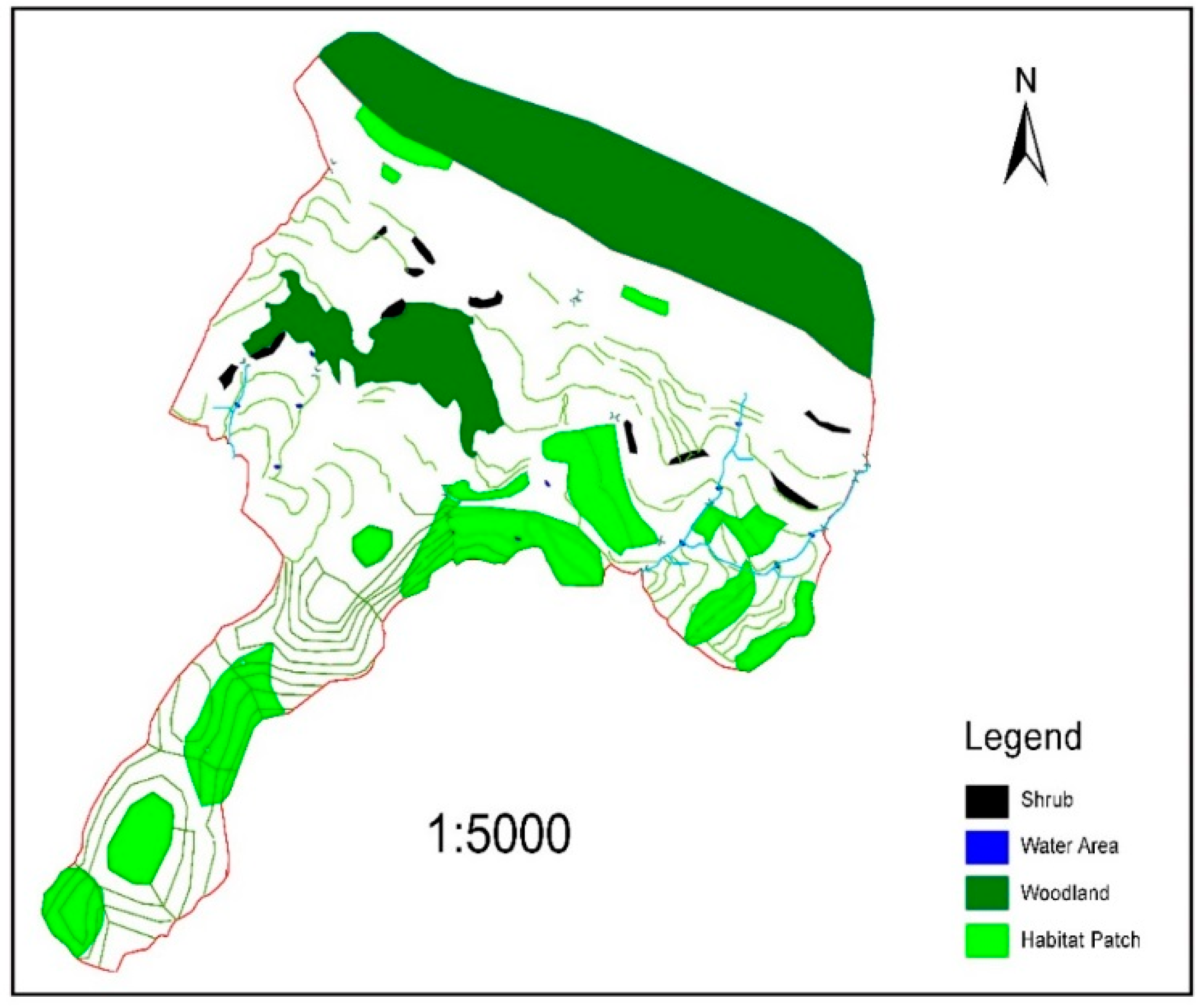
The habitat patches in the project area were identified via field surveys. The habitat patch sampling areas were demarcated, the number of species were counted, and the species richness was calculated to evaluate the flora species diversity. The number of species, projection area, frequency, and importance values of the species were calculated, and the relative importance of the different species in the sample was evaluated. The importance values of the species was calculated via Formula (2). With respect to the importance values, the growth of major species in the sampled communities, as well as the adaptation capabilities and disturbance avoidance strategies for these species, were estimated. Shrubs are the largest vegetation type in the karst mountain area. This vegetation type will form broad-leaved forests if there is successional progress; however, shrublands will form barren mountains if there is reverse succession. Therefore, habitat diversity is very important in terms of understanding the current situation of plant diversity, the mechanisms of diversity maintenance, and the interference of human activities on the biodiversity in the region. The ecological patches in the project area were identified as shown in Figure 2.

The importance values of the ecological patch communities in the project area are as follows

Table 6. Species richness and importance values of ecological patches in the project area.

Habitat Patch	Scrub-Grassland Community	Richness	Major Species Composition	Importance Value
1	Hornbeam privet	3.08	Hornbeam, privet, Itea yunnanensis, Platycarya longipes	66.50
2	Ulmus parvifolia, ailanthus	2.59	Ulmus parvifolia, ailanthus, Simon poplar, privet, tung tree	9.21
3	Rhamnus heterophylla	2.38	Rhamnus heterophylla, Viburnum foetidum, camellia	39.02
4	birchleaf pear, Rhamnus heterophylla	2.88	birchleaf pear, Rhamnus heterophylla, Viburnum foetidum, camellia	31.98
5	Whitebark, Rhamnus heterophylla	4.05	Whitebark, Rhamnus heterophylla, firethorn	36.23
6	Itea yunnanensis, Cotoneaster microphyllus	3.15	Itea yunnanensis, Cyclobalanopsis glauca, Coriaria sinica	48.44
7	Rhamnus heterophylla	2.21	Rhamnus heterophylla, Viburnum foetidum, Camellia, locust	31.86
8	Rhamnus heterophylla, firethorn	1.91	Rhamnus heterophylla, firethorn, Rosa cymosa	42.54
9	Melia azedarach, ailanthus	0.69	Melia azedarach, ailanthus, Campylotropis polyantha	38.44

.

Based on the composition of the sampled shrub communities and the importance values of the species, the dominant flora comprise plants that have relative strong adaptability, those that are drought resistant, and those that favor calcium, such as Rhamnus heterophylla and Hypericum uralum. Some tree species grow during the shrub community stage. The top stage of succession is difficult to reach due to harsh habitat conditions. Many primordial forest communities gradually degenerate into the shrub community and even bare stone land because of ornamental cultivation and grazing activity. Therefore, when ranking the main species by their importance value in a given habitat, the higher the importance value is, the stronger the adaptability of that species to the environment and the better the species resilience ability is, and vice versa.

Regarding the indexes selected by the above evaluation system, the greater the value is, the better the indexes that play a positive role in ecological sensitivity. The quantitative formula for this phenomenon is as follows:

$$A_i=\left(X_i-X_{i}min\right)/\left(X_i,max-X_i,min\right)$$

(10)

In the formula, A_i is the standardized index value, X_i represents the raw data, X min represents the minimum value of the raw data, and X max represents the maximum value of the raw data.

After the data were normalized, the ecological value of each landscape type was obtained by the weighted average method.

3.2. Landscape Pattern Index Calculations

Parcel information was extracted from the land use status map of the project area at a scale of 1:5000; a land parcel is a patch within the landscape pattern land consolidation process, which aims to increase agricultural productivity by reducing the area of inefficient farms while increasing the land area of efficient farms [64,65]. This process inevitably involves the merging and adjustment of land parcels. The land property rights in the project area belong to one village collective, but different land parcel use rights belong to different farmers or households (this is related to the political system in China, where land cannot be privately owned). After land consolidation, land use rights will be readjusted or exchanged based on farmer willingness. The land parcel map (Figure 3) served as a data source for analysis. The total project area is 32.37 hm². Division of this area into a 30 m × 30 m grid resulted in 358 cells, which served as evaluation units.

For each type of landscape patch, the average shape index, maximum area index, and habitat connectivity (cohesion index) were calculated with the land use status map via FRAGSTATS 3.3 and ArcGIS software. After the patch type level is chosen, the landscape pattern index can be calculated directly by the software according to Formulas (3)–(5). The landscape characteristics of the project area are shown in

Table 7. Landscape pattern indexes for the project area.

Landscape Pattern Index	Arable Land	Woodland	Corridors	Construction Land	Grassland	Rocky Desertification Land
Largest patch index	37.45	4.71	0.15	0.36	0.72	0.18
Mean shape index	2.78	2.49	8.78	1.38	1.54	1.48
COHESION	99.32	78.15	88.13	66.21	96.67	99.52

.

The largest patch in the project area comprised cultivated land. The ratio of the largest cultivated land patch to the whole landscape area is 37.45%, which indicates that cultivated land is the main landscape type in the project area. Because the project area is located in a karst mountain area, the shape of the cultivated land patch is not very regular. However, the connectivity between patches is relatively high. Therefore, keeping the arable land patches linked together in land consolidation is very important. The area of corridors in the landscape is small, and this land type is scattered and exhibits a very irregular shape. Scattered corridors should be consolidated and merged, and during the process of land consolidation, the connectivity of corridors should be strengthened to facilitate the connectivity of species and energy flow. Rocky desertification land is fragmented; however, the connectivity between patches is relatively high, and the shape is relatively regular. Thus, this land type can be reorganized by merging and centralizing.

3.3. Calculation of the Ecological Risk Degree Index

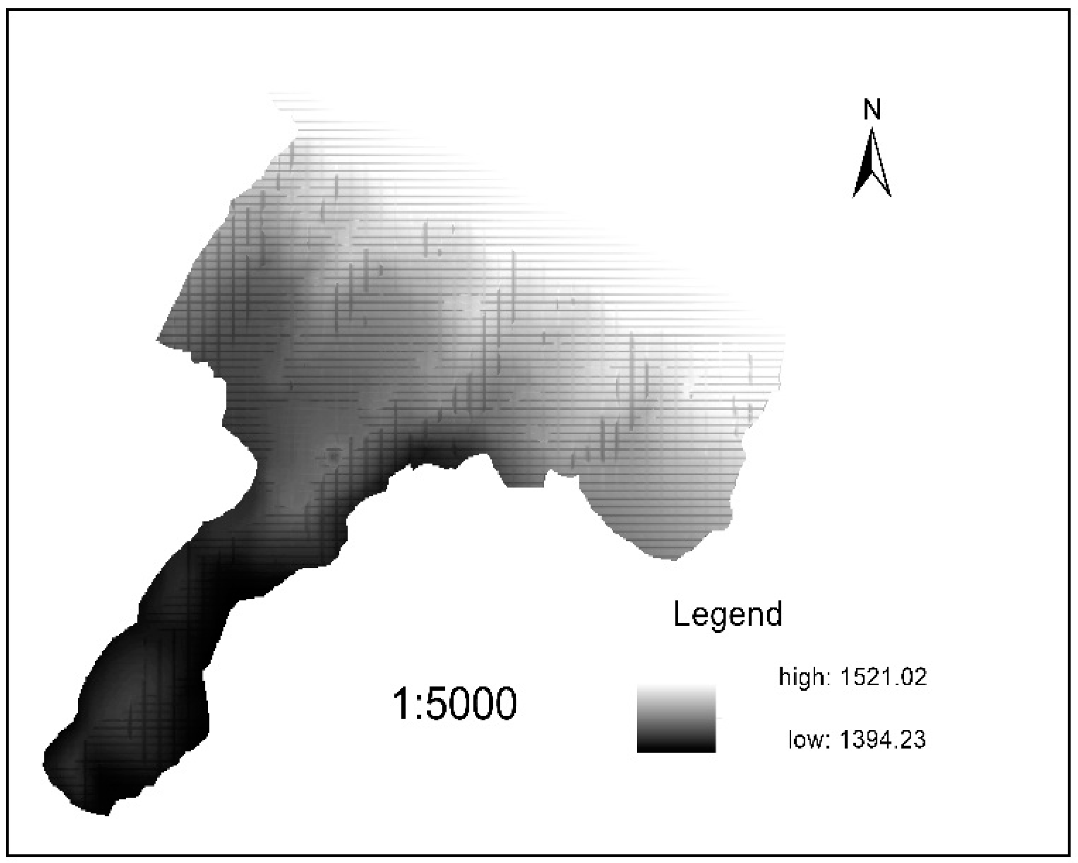
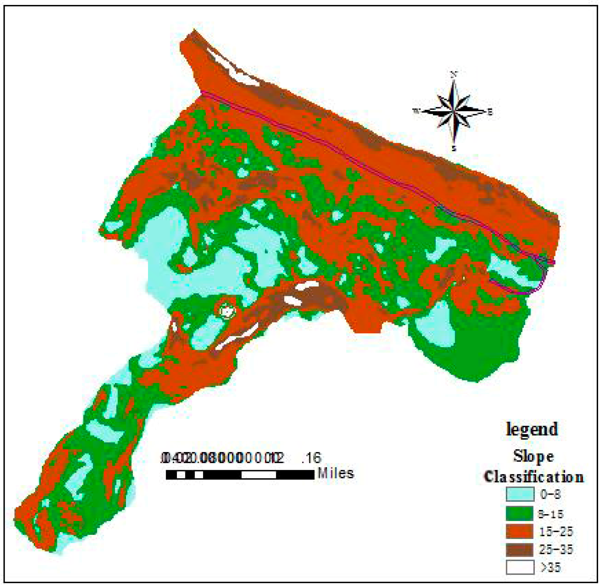
The average annual precipitation of the project area is 1205.1 mm, and the precipitation is unevenly distributed throughout the year. The precipitation is concentrated mainly in the summer, especially during June and August. The slope value for the project area was extracted from the DEM (Figure 4). The slope rating assignments were categorized as follows: a slope value >35° indicates an extremely sensitive area; a slope value = 25–35° indicates a highly sensitive area; a slope value = 15–25° indicates a moderately sensitive area; a slope value = 8–15° indicates a lightly sensitive area; and a slope value = 0–8° indicates a weakly sensitive area. The slope values for the project area are shown below in Figure 5.

The land use sensitivity level is calculated by assigning each land use type a single-factor sensitivity grade (Table 1). Bare rock land without vegetation is extremely sensitive to soil erosion. Farmland and grassland are highly sensitive to soil erosion, followed by woodland and corridors. Construction land is not sensitive to soil erosion.

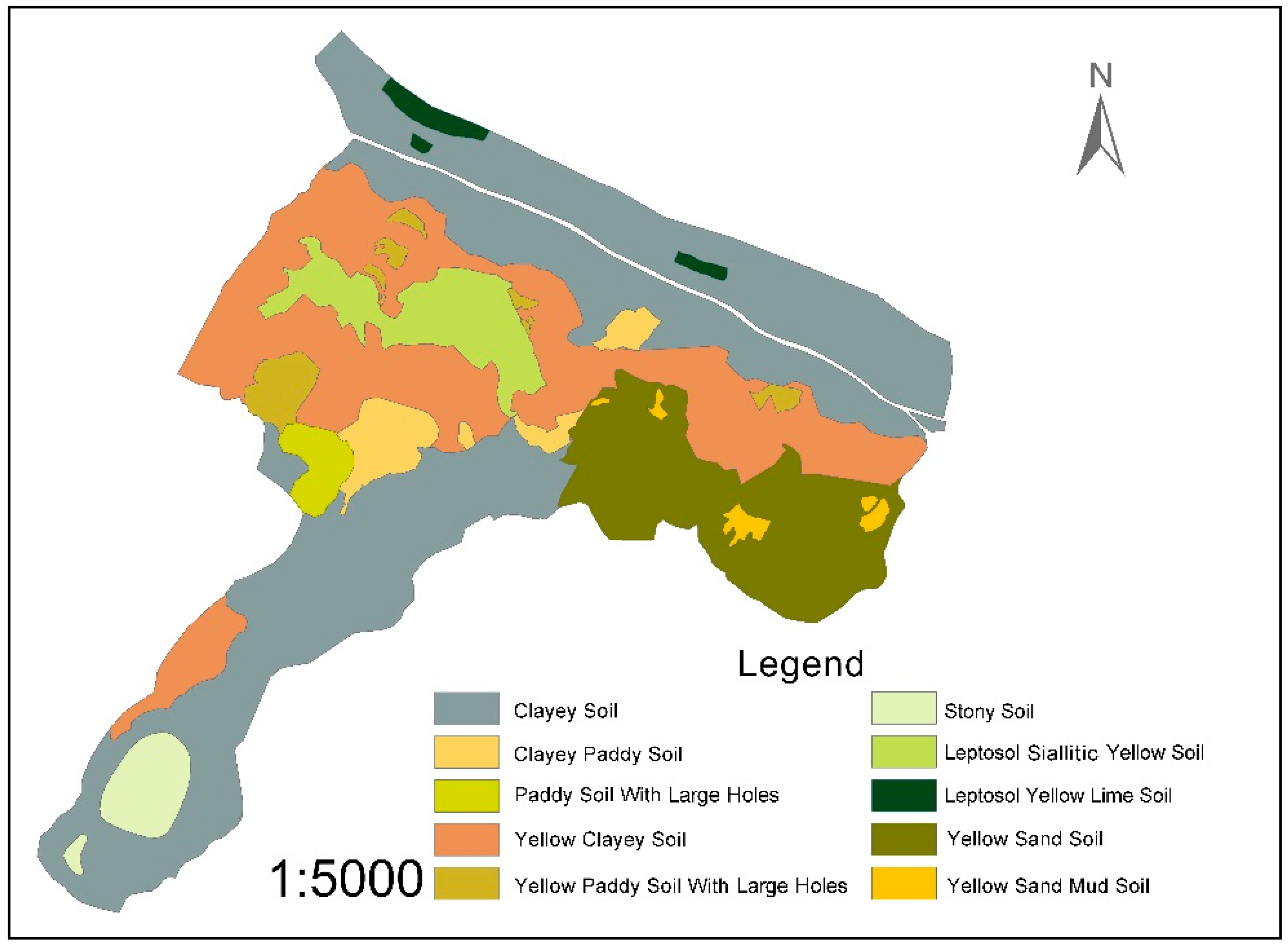
Yellow soils, calcareous soils, and paddy soils are the main soil types in the project area. Eighteen plow-layer soil (humus layer) samples were collected for analysis, and there were clear differences among the different types of soils. In the dry farmland, the yellow sandy soil texture comprises a sandy loam and silt clay loam. The texture of clayey soil is more viscous, and the texture changes between loamy clay and clay. The texture of yellow clayey soil is a mixture of loamy clay and sandy clay. In the paddy soil, the yellow sand mud soil has a clay loam texture. Regarding the texture of the two kinds of natural soil, lime soil is relatively viscous, whereas yellow soil is relatively loose. Silt is the most sensitive soil type. A sand–silt soil texture indicates a highly sensitive type of soil. Loamy soils exhibit medium sensitivity, and soil with a clayey texture are mildly sensitive; however, stony soils are not sensitive. The soil classification system for the project area is shown in

Table 8. Soil classification system for the project area.

Soil Type	Subclass Soil Type	Soil Genus	Soil Species	Area (hm2)	Ratio (%)
Yellow soil	Yellow soil	Siallitic Yellow soil	Leptosol Siallitic Yellow soil	1.82	5.64
			Yellow sand soil	4.25	13.15
	Subtotal			6.21	18.79
Lime soil	Yellow lime soil	Yellow lime soil	Leptosol yellow Lime soil	0.34	1.05
			Stony soil	0.81	2.50
			Clayey soil	14.35	44.40
			Yellow clayey soil	8.30	25.66
	Subtotal			23.80	73.61
Paddy soil	Submerged paddy soil	Yellow sand Mud soil	Yellow sand mud soil	0.23	0.72
		Paddy soil with large hole	Clayey paddy soil	1.01	3.12
			Paddy soil with large holes	0.41	1.26
			Yellow paddy soil with large holes	0.81	2.50
	Subtotal			2.46	7.60
Total				32.33	100.00

, and a distribution map of the soil types is presented in Figure 6.

The ecological risk stress index for project area was calculated according to Formulas (6) and (7) in conjunction with the parameters in Table 1. Because this index has negative effects on ecological sensitivity, the smaller the value is, the better the value. The quantitative formula is as follows:

$$A_i=\left(X_i,max-X_i\right)/\left(X_i,max-X_{i,}min\right)$$

(11)

In the formula, A_i is the standardized index value, X_i represents the raw data, X min represents the minimum value of the raw data, and X max represents the maximum value of the raw data.

After the data were normalized and the calculations were performed, the ecological risk stress index was obtained by the weighted average method. The weights were ultimately calculated in accordance with Formula (8), the ecological sensitivity was evaluated via Formula (9), and the sensitivity levels were classified.

4. Discussion

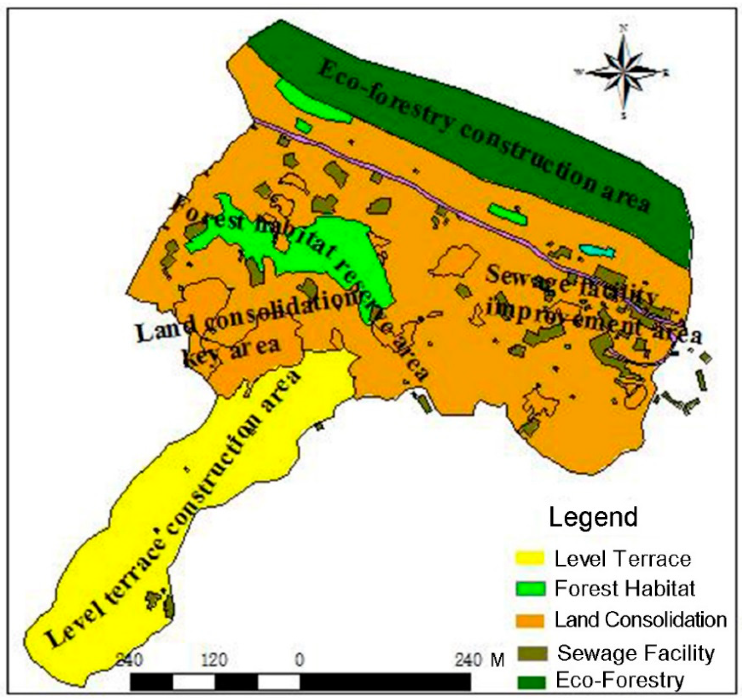
Ecological values are calculated by the landscape pattern indexes and the degree of ecological risk in the project area according to the weight assignments. The sensitivity grades of various landscape patches in the project area were classified. The higher the ecological sensitivity value is, the more sensitive the patch. Ecologically sensitive areas have an ecologically sensitive value >0.9. Ecological sensitivity values of 0.6–0.9 indicate a medium ecological sensitivity area, and values <0.6 indicate a low ecological sensitivity area. The zoning of the project area (Figure 7) and land consolidation engineering plan based on the ecological sensitivity evaluation in the project area is shown in

Table 9. Ecological sensitivity zoning in the project area and the optimal direction for land consolidation.

Zoning	Eco-Value	Landscape Pattern Characteristic	Ecological Risk	Optimal Direction
Zone 1 of high eco-sensitivity	0.95	Rocky desertification land with a bare surface and slope >25°	Soil and water loss, soil erosion risk	Vegetation restoration, shrubs and woodland planting area
Zone 2 of high eco-sensitivity	0.90	Grassland with a slope >25°, little vegetation and single species	Soil erosion risk	Vegetation restoration, forest community planting area
Zone 1 of medium eco-sensitivity	0.75	Farmland is the main landscape type	Risk of soil, erosion in some sloped cultivated land	Key area of land consolidation, level terrace construction area
Zone 2 of medium eco-sensitivity	0.68	Roads, corridors and ridges are the main landscape types	Connectivity performance needs to be optimized	Ecological corridor construction area
Zone 3 of medium eco-sensitivity	0.71	Residential and poultry farms are the main landscape types	Water pollution risk	Sewage facility improvement area
Zone of low eco-sensitivity	0.3	Woodland is the main landscape type	Good connectivity	Forest habitat, marginal vegetation conservation area

.

Bare rock and grassland are the main landscape types in the highly ecologically sensitive zones 1 and 2. These zones are located on a mountain in the northern region of the project area, which accounts for 48.5% of the total project area. The slope is between 45 and 60°, and the elevation is between 780 and 820 m a.s.l. The ground is exposed and has both a thin soil layer and relatively steep topography. Water and soil loss occur easily, especially on rainy days. The optimal plan for these zones under land consolidation engineering is the restoration of vegetation and the planting of forests.

Irrigated paddy fields and dry land are concentrated in the medium ecological sensitivity zone 1. The total area of irrigated paddy fields is 2.24 hm² and that of dry land area is 23.60 hm². Farmlands are distributed mainly in the central part of the project area and have a slope of 1–25°. The project area is in a typical Southwest China mountainous rocky desertification area, and there is a risk of soil erosion in the areas where the slope is steep. Karst land and grasslands rank second in terms of ecological stress. The patches are broken, and the facilities in these regions are simple and crude. The optimal plan for these areas involves substantial land consolidation.

Roads, ditches, ridges, and buffer areas are the main landscape types in the medium ecological sensitivity zone 2. The proportion of surface vegetation coverage is low, and there is some soil erosion risk. There is little vegetation coverage on both sides of the road, and gymnosperms include mainly cycads and Platycladus orientalis. Some native species are distributed on both sides of the ridges and roads, including Villous amomum, sweet potato vines, and Chinese prickly ash. The herbs in the paddy fields and ditches grow well and exhibit a high species richness. Arthraxon hispidus and bermudagrass (Cynodon dactylon) communities become present on some paddy field ridges after rice harvest. There are some Villous amomum, Chinese prickly ash and Aster ascendens Loisel, Alternanthera sessilis R.BrBougainvillea glabra Choisy, Calystegia hederacea Wall., Plantago major Linn., and others on the sides of dry croplands. Pangolins, spiders, and frogsare active in the herbaceous scrub next to paddy fields and ditches; these organisms maintain the balance of the ecosystem of the project area. Thus, during the process of land consolidation engineering, the following items are necessary: (1) The barriers to species migration and dispersal originating from artificial roads should be removed (an ecological corridor was constructed to link field roads, farm tracks and fields, accounting for 11.3% of the total project area); (2) Water ponds, pools, natural gullies, and their buffer zones should be designed as ecological islands and key construction areas for providing habitats or temporary habitats for living creatures.

Buildings and farmers’ livestock feeding facilities compose the main landscape type in the medium ecological sensitivity zone 3. Land consolidation can either change farmers’ residences or disturb their daily lives. However, owing to the lack of planned sewage channels for livestock excrement and household sewage, arbitrary discharge can pollute soil, groundwater, and vegetation habitats. Therefore, this region is best suited for a sewage channel construction area.

Woodlands are the main landscape type in the low ecological sensitivity zone. This region is also the soil and water conservation and ecological system stabilization area. The main threat to this area is that of farmers who have opened a path through the woodlands for their convenience; these paths have disturbed and destroyed some woodland ecosystems. This zone is planned to encompass both forest habitats and a marginal vegetation conservation area, and artificial roads are to be removed. The natural forest habitat should be restored, and a buffer zone should be established around the woodlands.

On the basis of the identification and maintenance of the optimal ecological pattern in the land consolidation project area, this study focuses on developing a comprehensive solution to regional eco-environmental problems. On the basis of research on natural ecological processes and ecosystem function, a series of ecological safety thresholds was determined. Furthermore, ecological process maintenance and control were proposed. On the basis of the evaluation of ecological sensitivity, factors such as ecological source land, the presence of ecological corridors, and a high degree of ecological risk stress were evaluated, and the project area was divided into an ecologically sensitive high-value area, middle-value area, and low-value area. The land consolidation zoning plan and engineering measures are reasonable. The research indexes supplement the landscape spatial pattern, and the factors of ecological risk stress take ecological processes into consideration, providing a spatial approach to ecological restoration and management in land consolidation activities.

5. Conclusions

This article evaluates ecological sensitivity based on GIS technology, landscape ecology theory, and the evaluation of possible disturbances and potential natural ecosystem service losses. To avoid losses in biodiversity or regressive succession in karst communities because of artificial disturbance, land consolidation activity should be optimized according to the ecological characteristics of each zone and adjusted to local conditions. Ecological values, landscape pattern indexes, and ecological risk evaluation constitute an effective way to construct an ecological sensitivity evaluation index. The coefficient of variation method and a comprehensive sensitivity rating evaluation method were very useful in calculating the corresponding weights and results in this study. The consolidation project area is divided into high ecological sensitivity zones, medium ecological sensitivity zones, and a low ecological sensitivity zone. The optimal direction for land consolidation engineering in each zone is proposed according to the natural geographical characteristics and ecological sensitivity of each zone.

When using an ecological sensitivity analysis and for optimizing the consolidation of land parcels, it is helpful to break from traditional land consolidation methods that focus on increasing cultivated land area as the sole object and pay attention only to economic benefits while neglecting ecological benefits. Ecological sensitivity analyses reflect the reaction of ecological systems to disturbances from human activities and changes in the natural environment to a certain extent. This research can provide a reference for environmental protection and land management decision-making. This paper focuses on ecological value, landscape pattern indexes, and the degree of ecological risk, all of which may be affected by land consolidation, as the main evaluation indexes. Other indicators must be considered in future research.