Article

Stationary Forestry with Human Interference

by
Petri P. Kärenlampi
Faculty of Science, University of Eastern Finland, PO Box 111, FIN-80101 Joensuu, Finland
Sustainability 2018, 10(10), 3662; https://doi.org/10.3390/su10103662
Submission received: 17 August 2018 / Revised: 26 September 2018 / Accepted: 5 October 2018 / Published: 12 October 2018
(This article belongs to the Section Environmental Sustainability and Applications)

Abstract

:
Here, we present stationarity criteria for forest stands and establish ecological embodiments using an empirical stand development model. We introduced human interference in terms of diameter-limit cutting. Financial sustainability was investigated as a function of the cutting limit diameter. It was found that nonoperative capitalization along with its appreciation rate dictates the sustainability of management practices. In the absence of nonoperative capitalization, stationary forestry produces high capital return rates at a rather small volume of growing trees. In the case of large but constant nonoperative capitalization, a large operative capitalization resulting in a large harvesting yield provides the best capital returns. A high nonoperative appreciation rate requires a small volume of growing trees.

1. Introduction

Multiannual plants are often produced in growth cycles, including terminal harvesting and artificial or natural regeneration [1,2,3]. However, that is not the only option. It is also possible to maintain a continuous cover of plants [4,5,6,7,8]. A few investigations indicate that continuous-cover forestry has particular benefits [9,10,11,12,13,14,15,16,17]. As a special case of the continuous-cover process, a stationary system may appear. A stationary system is supposed to display some kind of a demographic equilibrium [18,19,20,21,22,23]. In principle, a stationary stand may develop naturally, provided the system is given enough time for transient effects to level off. However, in quite a few cases, transient times in natural development may be significant, resulting in scarcity of naturally developed stationary states [22,23,24,25].
It has been postulated that in a natural state, the appearance frequency of trees would decay exponentially as a function of tree size [26,27,28]. However, we are not aware of any criterion of stationarity that would specifically produce exponential distributions. Exponential tree size distribution within a forest stand may be approached through specially designed harvesting schedules [8,29,30,31]. It however appears that such tailored systems are not stationary but in some kind of transient state [20,32].
In this paper, we discuss systems that fulfill a stationarity criterion, because of their conceptual simplicity and practical implementability. We concentrate on financial capital return in stationary forestry. We distribute capitalization to operative and nonoperative capitalization and investigate the latter’s effect of magnitude on financial return. It is worth noting that Buongiorno and Michie [12] applied a similar kind of growth model but with a very different economic treatment (cf. [33]). We do not discuss any net present value of cash revenues but describe forest economics in financial terms only.
First, we establish stationarity conditions for the size distribution of forest trees. The established steady-state equations were then parameterized using a Norwegian empirical model for the growth and mortality of Spruce trees, as well as recruitment of new trees [24,34]. The outcome is a description of a natural stationary state. Provided dying trees can be harvested, the natural state produces revenue corresponding to the financial return of the bound capital. However, when only harvesting dying trees, the volumetric yield is small. Introducing diameter-limit cutting, in addition to removal of dying trees, produces another stationary system, now with human interference. The effect of capitalization on the financial return is investigated with a variety of cutting-limit diameters.
Nonoperative capitalization due to excess demand for real estate, recreational values, speculation for future real estate values, etc., may well evolve over time. In the final section of this paper, we discuss the effect of the eventual appreciation of the nonoperative capitalization on the financial return in stationary forestry.

2. Methods

2.1. Stationary Stand of Forest Trees

A stationary structure requires stationary distributions of population properties. Let us define stationary conditions on the basis of three processes of diameter ingrowth, diameter outgrowth, and mortality. The process of outgrowth obviously must be related to ingrowth into another group. The size distribution of trees can be stationary only if the number of individuals involved in the three processes sums up to zero. Consequently, a stationarity condition is
I d 5 ( D i 1 ) n ( D i 1 ) I d 5 ( D i ) n ( D i ) m ( D i ) n ( D i ) = 0
where n ( D i ) is the number of trees in diameter class i, I d 5 ( D i ) is the probability that a tree survives and grows into the next diameter class, and m ( D i ) is mortality. Such a stationarity criterion is rather generic and appears in a variety of contexts. For forest stands, we established the criterion independently before finding out that it has been several times mentioned by Schütz [18,20,21] and applied to the growth of US Northern hardwoods by Buongiorno and Michie [19].
Taking the indices i as positive natural numbers in Equation (1), i − 1 becomes ill defined with the smallest value i = 1. In other words, for the smallest diameter class, we need a boundary condition
R I d 5 ( D 1 ) n ( D 1 ) m ( D 1 ) n ( D 1 ) = 0
where the first term R corresponds to the number of trees recruited into the smallest diameter class.

2.2. Empirical Model Applied

In order to solve the tree size distribution in a stationary state according to Equations (1) and (2), the three functions appearing in the equations have to be clarified. We utilized the empirical model of Bollandsås et al. [24,34]. The three functions become
I d 5 ( D i ) = a 1 + a 2 × D i + a 3 × D i 2 + a 4 × D i 3 + a 5 × B A L ( D i ) + a 6 × S I + a 7 × B A + a 8 × L A T Δ
m ( D i ) = 1 1 + exp { 1 × [ b 1 + b 2 × D i × 10 + b 3 × ( D i × 10 ) 2 + b 4 × B A ] }
R = c 1 × ( B A ) c 2 × ( S I ) c 3 1 + exp { 1 × [ d 1 + d 2 × B A + 0.0655 × S I + d 3 ] }
where a k , b k , c k , and d k are constants, given in [24,34] and reprinted in Supplementary Materials. B A L ( D i ) is basal area in trees larger than D i , S I is site index (dominant height at 40 years of age), B A is total basal area, L A T is latitude, and Δ is diameter increment from diameter class i-1 to class i.
Within the underlying experimental material, the site fertility indices ranged from 6 to 26. We here intend to discuss the outcome of the model at three site fertilities, with fertility indices 11, 17, and 23. These values correspond to moderate, good, and very good sites. Fertilities poorer than 11 were neglected due to their marginal economic importance.

2.3. Effects of Human Interference

Let us now consider a case where a human interferes with the stationary state by a particular harvesting program of periodic character. Let us discuss a practice where trees larger than a particular diameter are periodically harvested. Then, Equations (1) and (2) are still valid in other diameter classes, but for the largest diameter class,
n ( D M a x ) = 1 2 I d 5 ( D M a x 1 ) n ( D M a x 1 )
The largest diameter class here corresponds to trees larger than the cutting limit diameter. Immediately after diameter-limit cutting, there are no such trees. However, some appear before the next diameter-limit cutting, and a simple approximation of a representative (or “average”) number of them is half of the number of ingrowth according to Equation (6).

2.4. Financial Methods

In order to discuss financial return rate, we need to introduce a financial potential function K. The financial potential corresponds to capitalization per surface area unit. The capitalization is distributed to operative and nonoperative capitalization. The operative capitalization corresponds to the monetary value of the standing trees as well as the nonamortized value of eventual forestry investments like regeneration investments, fertilizations, drainage expenses, etc. However, in this paper, we do not discuss any investments. The nonoperative capitalization corresponds to real estate value exceeding the value of trees and eventual nonamortized investments. Nonoperative capitalization may be due to excess demand for real estate in comparison to supply, recreational values, speculation for future real estate development, etc. (It is worth noting that generalized Faustmann formulae may contain variable land expectation values [35,36]. The generalized formulation could be used to assess the effect of real estate valuation on silvicultural practices [10]. However, such a treatment is not relevant for stationary forestry since there is no need for discounting). An eventual value of bare land is included in the nonoperative capitalization.
The monetary value of standing trees is constituted as the product of assortment volumes and assortment prices. The number of trees per surface area unit in any breast height diameter class is clarified by substituting any of Equations (3)–(5) into (1) and (2). It is noticed that the stand basal area contributes to any of the Equations (3)–(5). On the other hand, the stand basal area can readily be reconstituted from the tree diameter distribution resulting from Equations (1) and (2). We experiment with the stand basal area, and an iteration rapidly results as a stationary state where the input value is regained from Equations (1) and (2).
The stem diameter can be converted to trunk volume in a variety of ways. We simply applied the relationship given by Rämö and Tahvonen [14,37] for fertile spruce stands. Any breast height diameter was converted to the volume of two assortments—pulpwood and sawlogs—according to the appendix given by Rämö and Tahvonen [14,37]. The stumpage value of the assortments was calculated on the basis of stumpage prices given by Rämö and Tahvonen ([14], p. 1104).
The momentary capital return rate is the relative change rate of the potential function
r ( t ) = d κ K ( t ) d t
The net return rate d κ d t in Equation (7) here corresponds to the monetary value of the net growth rate of trees. In the case of operative investments, amortizations would be deducted from the gross growth rate. In case there are dying trees that are not harvested, their value is deducted. The number of trees growing to a larger diameter class was produced using Equation (3), along with the number of trees in any diameter class produced using Equations (1)–(5), as explained above. The trees transferred to a larger diameter class contained a larger amount of pulpwood and sawlogs according to the appendix of Rämö and Tahvonen [14,37]. The monetary value of the incremental assortment volumes was clarified according to stumpage prices by Rämö and Tahvonen [14]. Finally, the monetary net growth rate was integrated over all the diameter classes.
In Equation (7), there is a slight difference between κ in the numerator and K in the denominator relating to eventual operative investment or divestment. The potential (or capitalization) K is immediately affected by any eventual operative investment or withdrawal and then consequently becomes affected by amortizations. The net return rate d κ d t in the numerator, however, characterizes the growth rate in financial terms and thus is not immediately affected by changes in capitalization but considers eventual investments in terms of amortizations. In addition, changes in capitalization are likely to contribute to growth: investments probably increase growth rate, whereas withdrawals may reduce growth rate. Such effects, however, are not discussed here in detail since this study does not consider any investments.
In the stationary state, the potential K(t) does not evolve persistently but possibly experiences some fluctuation around its characteristic value. In the natural stationary state, in the absence of harvesting and of mortality offsetting growth, the change rate of potential d κ d t is zero, also resulting in constancy of the potential function K(t).
In stationary states with human interference, d κ d t is nonzero since potential created by growth does not rot in the ground but becomes harvested. On the other hand, K(t) is not strictly a constant but fluctuates around a characteristic value Kch, accumulated growth periodically being divested in terms of harvesting.
Let us then distribute capitalization K(t) to the operative capitalization O ( t ) and the nonoperative capitalization U ( t ) . Now, Equation (7) can be rewritten as
r ( t ) = d Ω + d U [ O ( t ) + U ( t ) ] d t
In Equation (8), the difference between Ω in the numerator and O in the denominator again relates to eventual operative investment or divestment. The capitalization O is immediately affected by any eventual operative investment or withdrawal and then consequently becomes reduced by amortizations. The net return rate d Ω d t in the numerator is not immediately affected by changes in capitalization. Correspondingly, the accumulated net yield Ω ( τ ) may differ from operative capitalization O ( τ ) in the occurrence of withdrawals (harvesting, etc.).
In stationary states with human interference, d Ω d t is nonzero since potential created by growth does not rot in the ground but is stored through harvesting of produced timber. On the other hand, O(t) is not strictly a constant but fluctuates around a characteristic value Och, with accumulated growth periodically being divested in terms of harvesting. Consequently, at a stationary state
r ( t ) d Ω + d U [ O c h + U ( t ) ] d t
Equation (9) reveals that in the case in which the operative capitalization is much higher than the nonoperative capitalization, the role of the latter vanishes. On the other hand, if nonoperative capitalization is much higher than operative capitalization, the role of the operative capitalization vanishes. In case the nonoperative capitalization is large but constant, the highest operative return might simply be the one corresponding to greatest average yield rate d Ω d t . The situation is more delicate if there is a nonvanishing time change rate of the nonoperative capitalization d U / d t .
The nonoperative capitalization U should be parametrized somehow. We chose to normalize it with the operative capitalization at the natural steady state. In other words, our measurement gauge for nonoperative capitalization was U O c h _ n a t . Now, provided the relative appreciation rate of nonoperative capitalization d U U ( t ) d t is known, it is possible to investigate the capital return as a function of cutting-limit diameter on the one hand and nonoperative capitalization on the other hand.

3. Results

3.1. Properties of the Stationary State

Figure 1 shows the number of trees within any diameter class in a stationary state on a spruce stand for three site fertility classes according to Equations (1)–(5). The only free parameter appearing in Equations (1)–(5) is latitude, which is given value 61.9.
The total number of trees of diameter in excess of 50 mm per hectare is 310, 346, and 383 for the tree site indices. The corresponding basal areas at breast height are 27.1, 32.5, and 37.3 m2/ha. An interesting feature in Figure 1 is that in the case of the lowest fertility, the size distribution is bimodal. As the growth rate decreases with size according to Equation (3), there is some crowding of trees at 475-mm diameter class. Increased mortality, according to Equation (4), however, reduces the appearance frequency of larger trees.
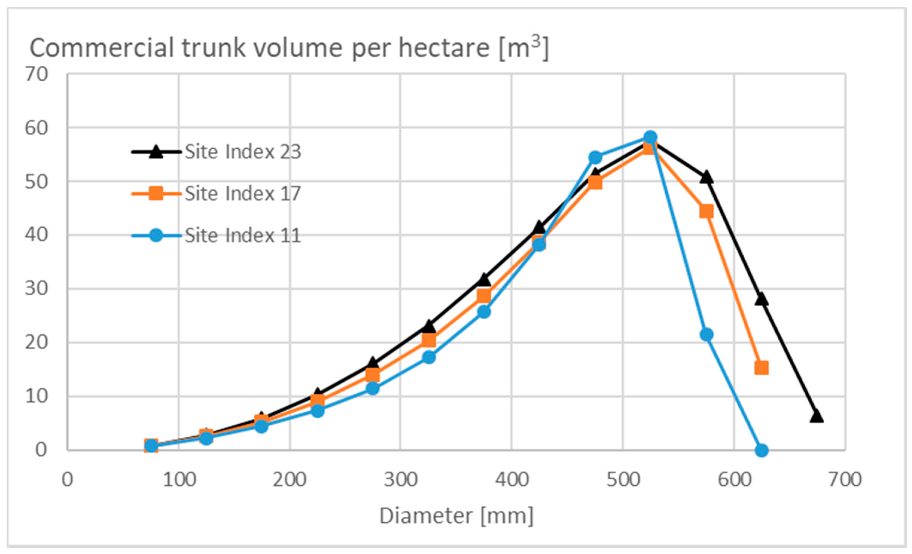
The commercially utilizable trunk volume in trees of different diameter classes is given in Figure 2. We found that the total commercial stand volume per hectare is 242, 285, and 326 m3/ha for the three fertility classes.
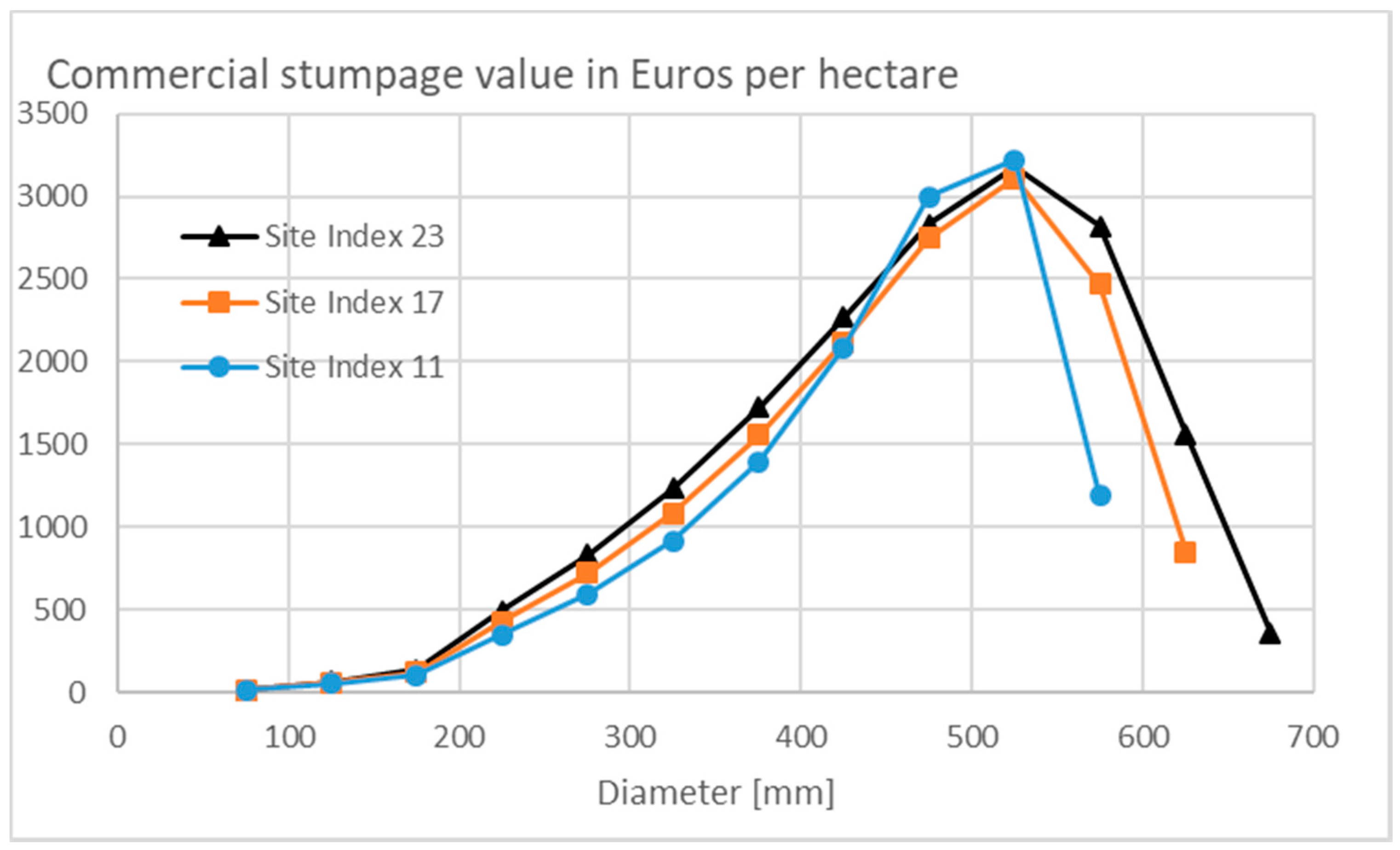
The stumpage value of the standing trees can be calculated on the basis of stumpage prices given by Rämö and Tahvonen [14]. The outcome is given in Figure 3. We found that the total stumpage value per hectare is 12,962, 15,278, and 17,516 Eur/ha for the three fertility classes.
According to Equation (1), the number of dying trees within any diameter class corresponds to the number of trees growing out subtracted from the number of trees growing into the class. In a stationary state, the commercial wood trunk volume remains constant. Correspondingly, in the absence of harvesting, the reduction of the volume of living trees through death equals volumetric growth (Equation (1)). The total amount of growth per hectare during a five-year period is 5.8, 11.4, and 19.4 m3 for the three site fertility classes. Correspondingly, the annual growth rate varies from 1.2 to 3.9 m3/ha.
It is of interest to compare the stumpage values of dying trees to the total value of standing trees. Provided the five-year growth can be technically harvested and yields the expected stumpage value, the annualized operative return of the capital standing on trees becomes 0.5%, 0.8%, and 1.2% for the three different site fertility classes. Obviously, gaining the full stumpage value requires that the harvester is a professional capable of identifying dying trees before they suffer any deterioration of commercial value.

3.2. Effects of Human Interference

The commercial volume of trees harvested within any five-year period in diameter-limit cutting is shown in Figure 4. The effect of human interference is introduced according to Equation (6), in addition to Equations (1)–(5). It is assumed that in the context of diameter-limit cutting, dying trees are removed from all diameter classes. Figure 4 shows that when the cutting limit approaches the diameter of the largest trees, the harvesting pattern approaches removal of naturally dying trees. With reduced cutting diameter limit, the proportion of harvesting volume from dying trees reduces rapidly. The greatest harvesting volume is gained at a cutting limit of 400–450 mm. With a smaller harvesting limit diameter, the harvesting volume becomes rapidly reduced.
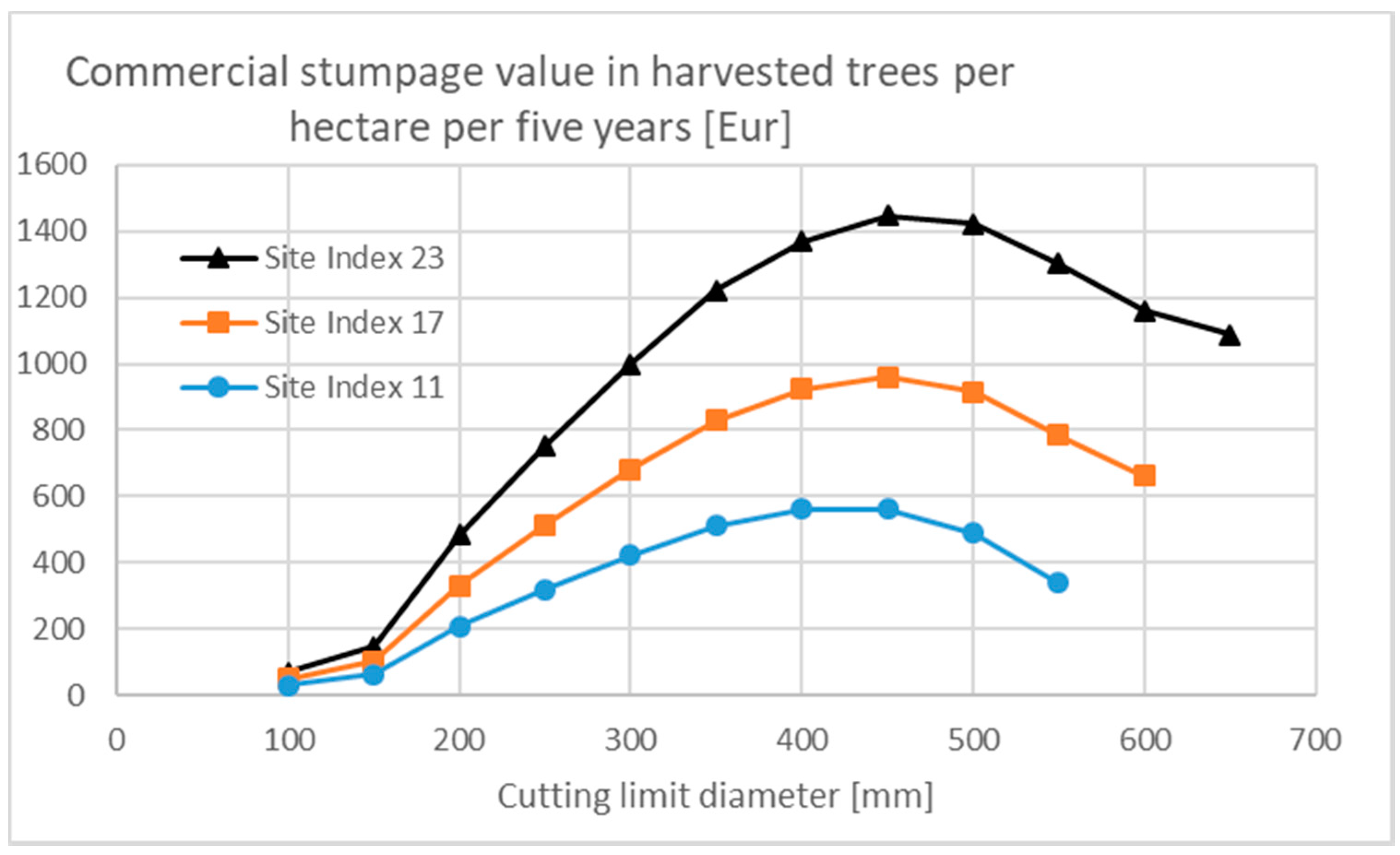
Commercial stumpage value of trees harvested in diameter-limit cutting within any period of five years is shown in Figure 5. The highest commercial value is gained with a cutting diameter limit of 450 mm. As a function of cutting diameter limit, the greatest increment of stumpage value is found between 150 and 200 mm, where sawlogs appear in the harvesting yield instead of merely pulpwood.

3.3. Financial Return Rate

3.3.1. Nonappreciating Nonoperative Capitalization

Let us first investigate the case where the time change rate of the nonoperative capitalization d U / d t equals zero. In this case, the numerator of Equation (9) only corresponds to the first term, which is closely related to Figure 5 but is here discussed on an annual basis. Even if the change rate of the nonoperative capitalization d U / d t vanishes, some amount of nonoperative capitalization U may appear in the denominator of Equation (9).
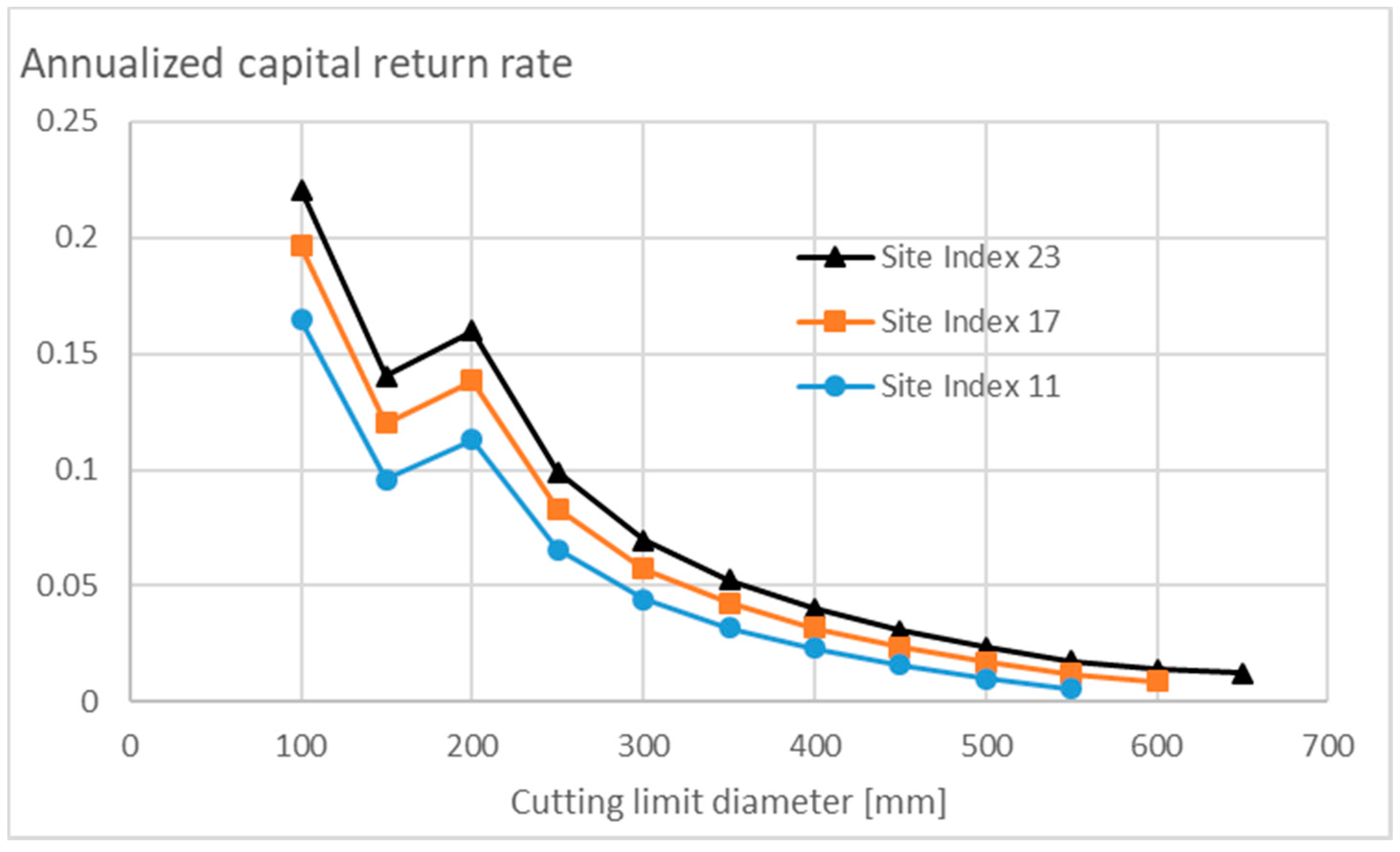
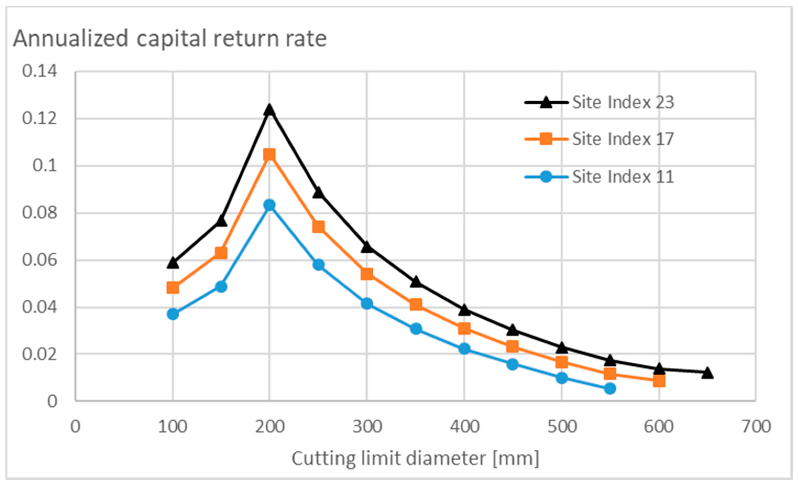
Figure 6 shows the capital return rate for vanishing nonoperative capitalization, i.e., U O c h _ n a t = 0 . We find that the greatest capital return rate is achieved by harvesting small trees. This is, however, problematic, since the volumetric harvesting yields according to Figure 4 are rather low.
Figure 6 shows that there is another peak value in capital return at the cutting limit of 200 mm, where sawlogs are first gained. However, the volumetric harvesting yields according to Figure 4 still are low.
Figure 7 shows the capital return rate for U O c h _ n a t = 0.01 . Interestingly, such a smallish nonoperative capitalization completely changes the financial profile. In the case of the 100-mm cutting limit diameter, the originally tiny capitalization increases significantly, and the relative capital return collapses correspondingly. On the other hand, in the case of the greatest diameter cutting limits, the capitalization increases only by 1%, and the decline of relative capital return rate is of a similar magnitude. However, according to Figure 7, the greatest capital return rate is achieved with a cutting limit diameter of 200 mm, where sawlogs are first gained.
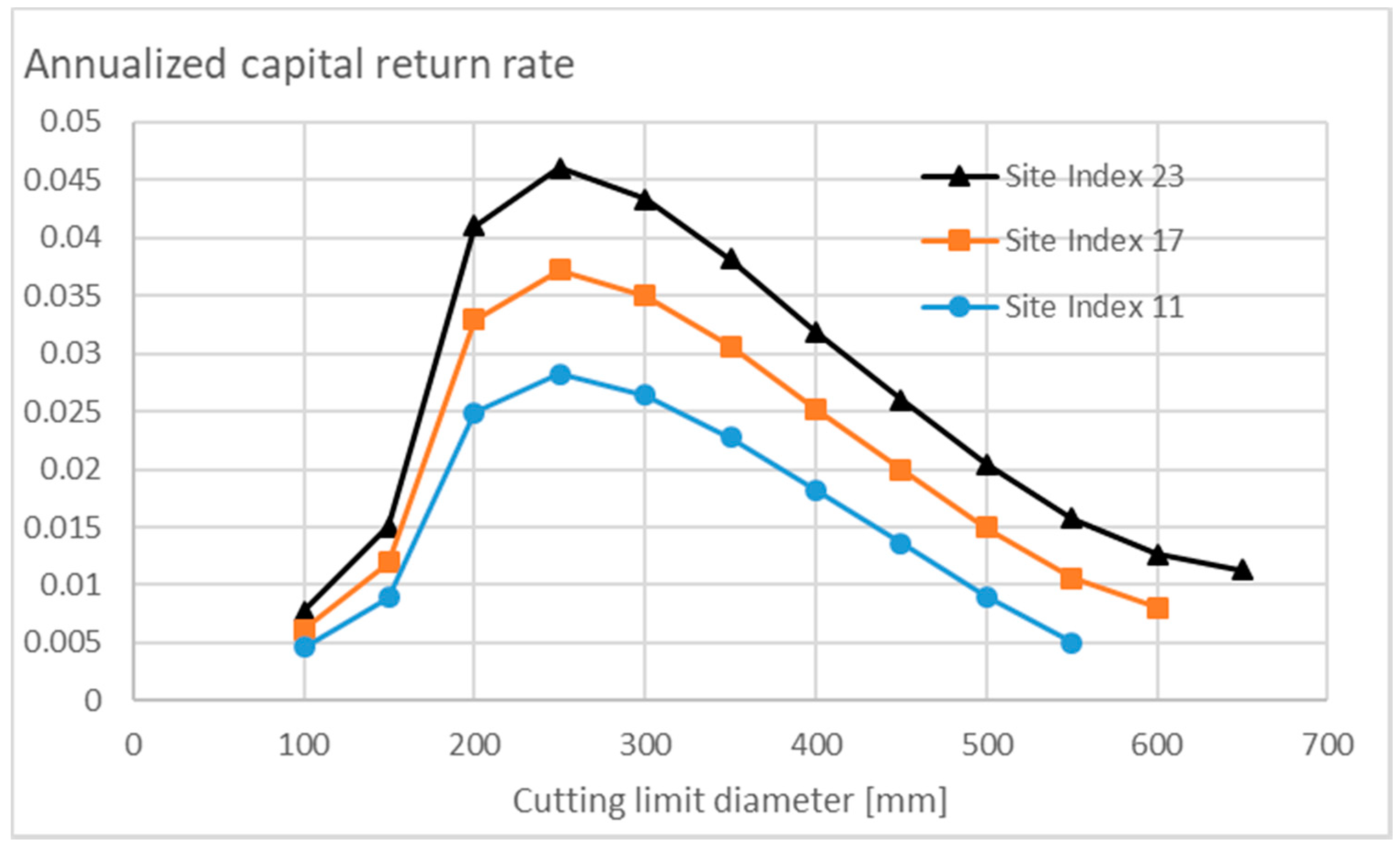
Figure 8 shows the capital return rate for U O c h _ n a t = 0.1 . In the case of the 100-mm cutting limit diameter, the capitalization is now 10 times greater than the one corresponding to Figure 7. On the other hand, in the case of the greatest diameter cutting limits, the capitalization increases only by 10%, and the decline of relative capital return rate is of a similar magnitude. According to Figure 8, the greatest capital return rate is achieved with a cutting limit diameter of 250 mm instead of 200 mm in Figure 7.
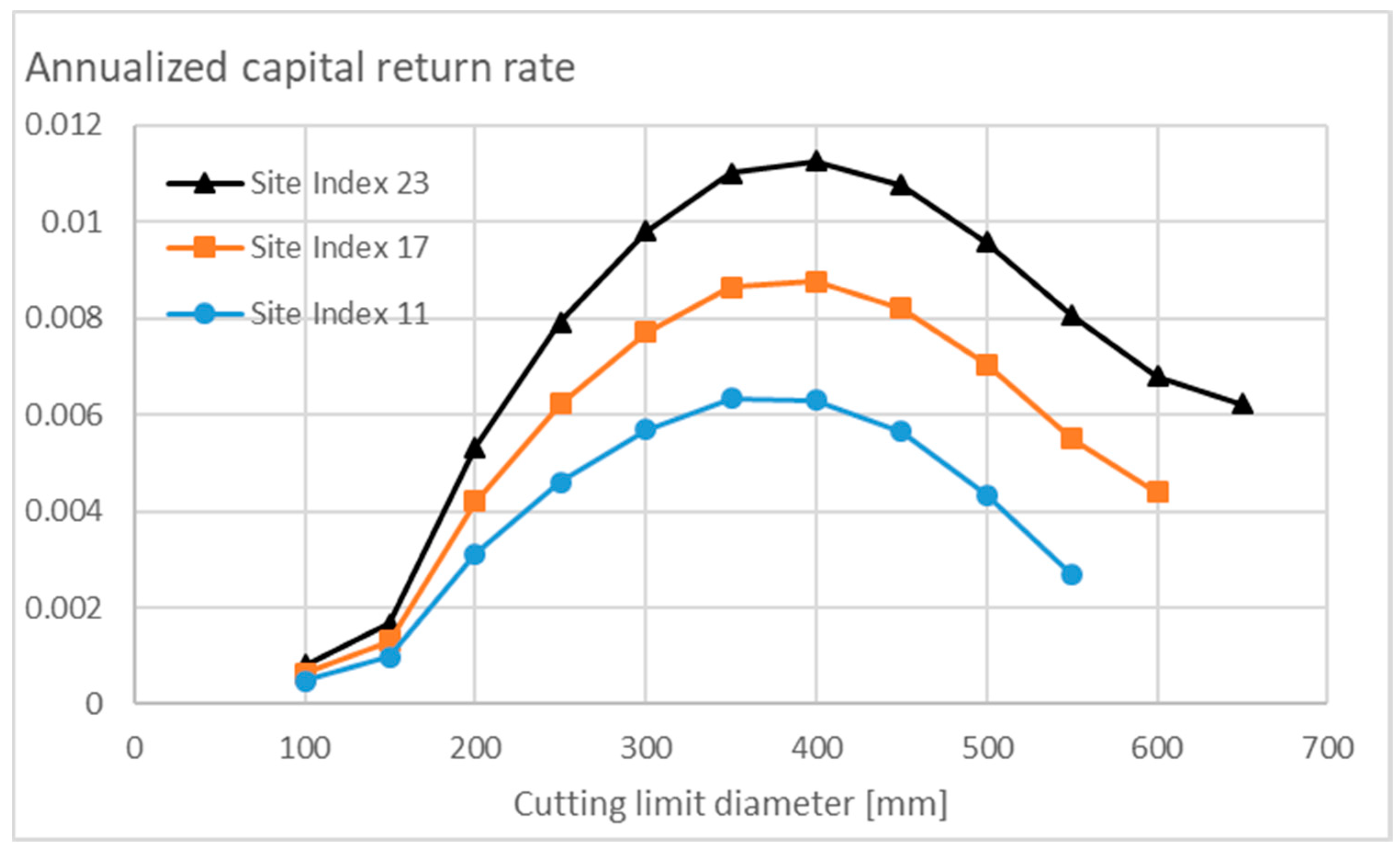
Figure 9 shows the capital return rate for U O c h _ n a t = 1.0 . In comparison to Figure 6, capital return rate is 300 times smaller at the smallest cutting limit diameter and halved at the greatest cutting limit diameters. The greatest capital return rate, even if small, is achieved with cutting limit diameters of 350–400 mm. Further increments in nonoperative capitalization would increase the cutting limit diameter corresponding to the greatest capital return to 450 mm, thus providing the greatest harvesting yield according to Figure 4 and Figure 5.

3.3.2. Appreciating Nonoperative Capitalization

A previous study indicates that in the case of periodic rotation forestry, appreciating nonoperative capitalization significantly reduces financially optimal rotation age [38]. This obviously is not the case in stationary forestry because no rotation age exists in a stationary growth process. However, it is obvious that the total capital return depends on the appreciation rate of nonoperative capitalization. Correspondingly, we investigated a few cases where the second term in the numerator of Equation (9) is also possibly nonzero.
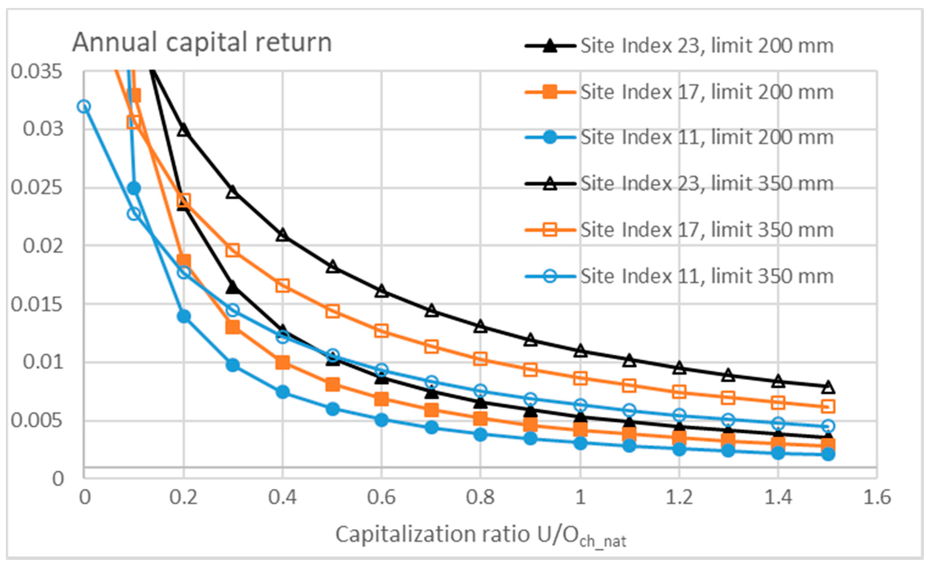
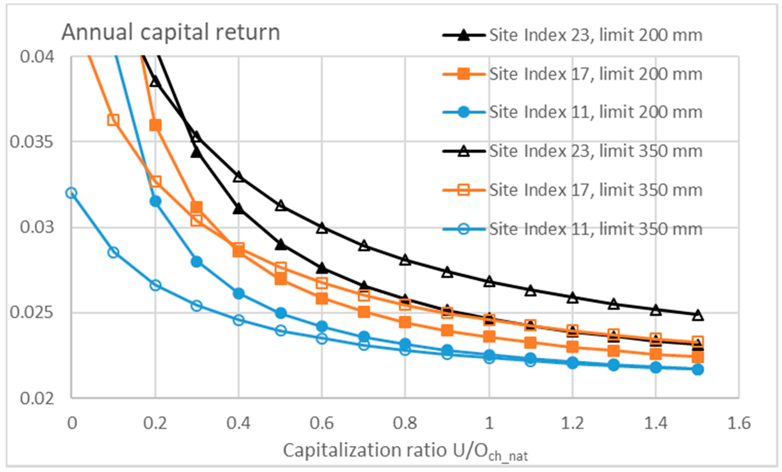
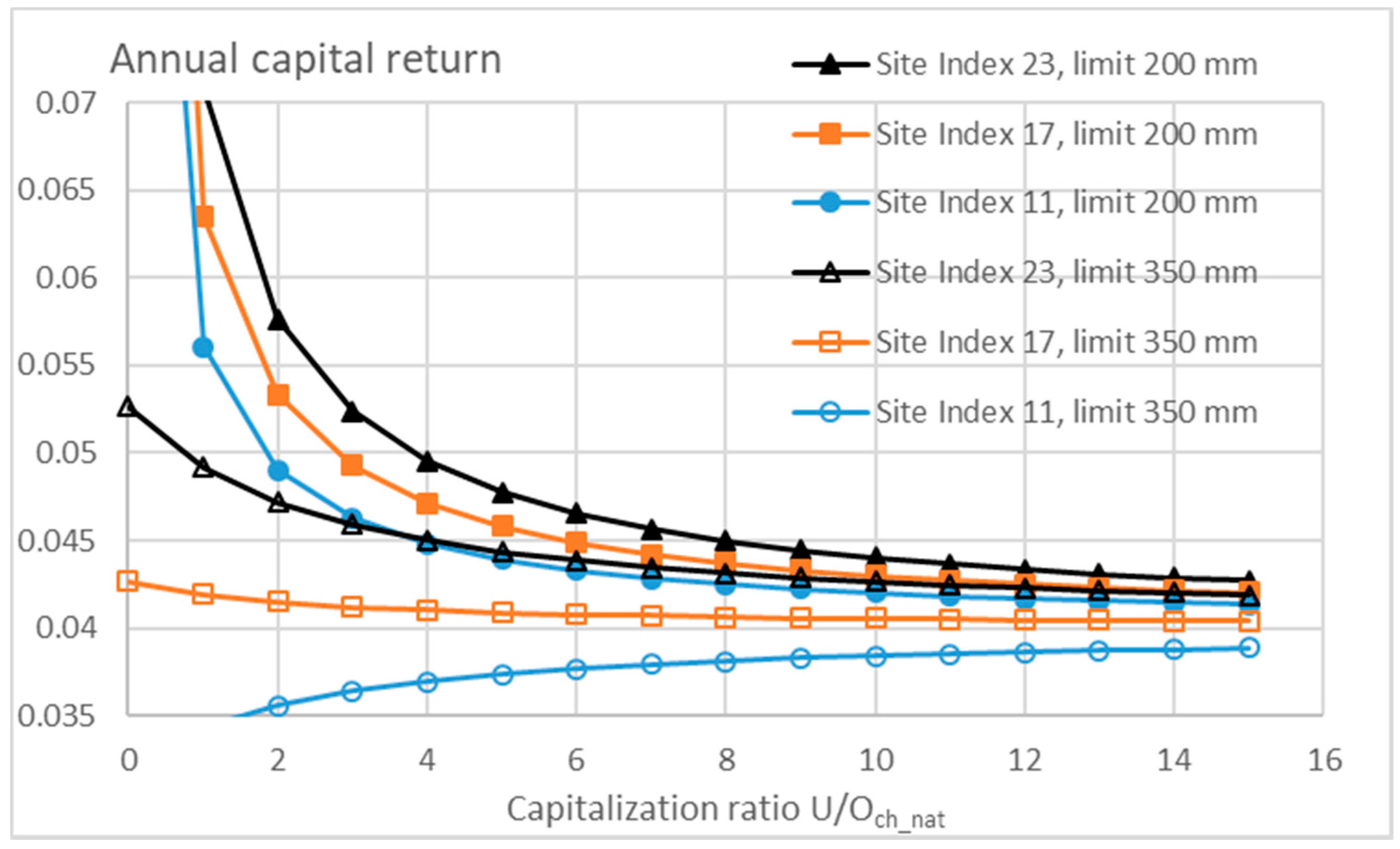
Motivated by Figure 7 and Figure 9, we report in Figure 10, Figure 11 and Figure 12 the evolution of capital return rate with two cutting limit diameters: 200 and 350 mm. We plot the capital return rate as a function of the capitalization ratio U O c h _ n a t . Annual appreciation rates of 0%, 2%, and 4% were used for the nonoperative capitalization in Figure 10, Figure 11 and Figure 12, respectively.
Figure 10 shows that with an annual nonoperative capital appreciation rate of 0%, harvesting large trees of sizes in excess of 350 mm yields a better capital return than harvesting small trees (200 mm) with capitalization ratios U O c h _ n a t greater than 0.1–0.2. It is worth noting that the bigger cutting limit diameter corresponds to more than doubled harvesting yield according to Figure 4 and Figure 5.
Figure 11 shows that with an annual nonoperative capitalization appreciation rate of 2%, harvesting large trees of sizes in excess of 350 mm yields a better capital return than harvesting small trees (200 mm) with capitalization ratios U O c h _ n a t greater than 0.3–0.4. However, that result applies only to high and intermediate site fertilities. In the case of the lowest site fertility, the capital return rates unify at high capitalization ratios: the high capitalization case of 350-mm cutting limit diameter never shows a greater capital return rate.
Figure 12 shows that with an annual nonoperative capital appreciation rate of 4%, harvesting small trees (200 mm) always produces a greater capital return than harvesting large trees of sizes in excess of 350 mm, regardless of capitalization ratio U O c h _ n a t . This result indeed significantly differs from Figure 10 and Figure 11 and indicates that appreciation of nonoperative capitalization plays a fundamental role in forestry finances.
It is of interest to note that in the case of the lowest fertility and higher cutting limit diameter, the capital return rate increases with increased nonoperative capitalization. A natural reason is that the return rate in the absence of nonoperative capitalization is below the 4% nonoperative appreciation rate (cf. Figure 10 and Figure 11).

4. Discussion

The empirical models (3)–(5) utilized in this study describe growth, mortality, and recruitment in a statistical sense. Significant scattering beyond modeled trends appears in any dataset [24]. Consequently, some amount of uncertainty in the present results obviously is related to the reliability of the used models. However, qualitatively, the appearance of slow recruitment, in accordance with Equation (5), appears to agree with quite a few observations [6,23,39,40,41]. Also, observations indicating a higher rate of recruitment exist [42,43,44].
The amount of trees in the stationary forest, in terms of number of individuals (Figure 1), appears rather small in comparison to nonstationary forest systems [7,11,14,17,45,46]. On the other hand, basal area and standing volume are more comparable (Figure 2). Growth rate is smaller than generally reported for comparative fertilities in nonstationary forestry (Figure 4) [7,11,14,17,45,46,47,48]. These observations are directly due to Equations (3)–(5). Especially, the recruitment rates given by Equation (5) appear rather slow, inducing stationary systems with a small number of trees.
All the empirical data used in this paper were taken from one single modeling of one large Norwegian dataset [24,34]. The present results may be due to the generic diameter distributions of the type shown in Figure 1. However, it would be of interest to compare with different tree species, climates, and regions. Quite a few investigations have been published reporting recruitment, growth, and mortality [5,47,48,49,50,51]. However, it apears that most of such modelings have been unsuccessful. A modeling should be considered unsuccessful if Equations of type (3)–(5) do not converge to a stationary structure according to Equations (1) and (2). A common reason for such failure appears to be an inappropriate description of mortality: in case growth rate diminishes but mortality does not increase, Equation (2) accumulates a large and increasing number of trees to large diameter classes. A positive exception, apparently, is the model by Buongiorno and Michie [12], which we hope to apply in the future.
Regarding the financial results of this paper, some of the results appear rather surprising. Firstly, in the absence of nonoperative capitalization, the best capital return rates are gained with rather small cutting limit diameters (Figure 6). However, the situation significantly changes with a small amount of nonoperative capitalization, with the best return being gained with a cutting limit diameter where sawlogs are first gained (Figure 7). A further increment of nonoperative capitalization, however, again changes the situation, with the best capital return rates being gained at much greater cutting limit diameters (Figure 8 and Figure 9). Such higher cutting limits provide greater volumetric and monetary harvesting yields in comparison to the previous ones (Figure 4 and Figure 5).
Still more interestingly, eventual appreciation of the nonoperative capitalization significantly contributes to the financial return. Figure 10 shows that in the absence of appreciation, small capitalization favors harvesting of smallish trees, whereas large capitalization favors large cutting limit diameters. However, the situation partially changes with a 2% annual appreciation rate (Figure 11). An appreciation rate of 4% completely changes the situation, favoring small cutting limit diameters corresponding to small operative capitalization. This obviously requires some kind of an explanation.
In order to explain the effect of the appreciation rate of the nonoperative capitalization, at least partially, let us process Equation (9) further. First, let us define two “pure” capital return rates as
g d Ω O c h d t
and
f d U U d t
Now, Equation (9) can be rewritten
r g + f U O c h 1 + U O c h
Before proceeding any further, we must remember that in Equation (10), the pure capital return rate depends strongly on Och. In addition, r depends strongly on U O c h _ n a t , even if f d U U d t would be zero. This dependency is clearly seen in Figure 10: with increasing capitalization ratio U O c h _ n a t , the larger cutting diameter limit corresponding to greater operative capitalization Och overtakes the smaller in terms of total capital return rate r. So, why does this not happen in the case of Figure 12, where f d U U d t is nonzero?
Obviously, the difference between Figure 10 and Figure 12 can be explained in terms of Equation (12). In case f d U U d t = 0 , increment in Och in the denominator tends to increase r. However, if f d U U d t essentially differs from zero, that increment is less pronounced, 1 O c h now appearing also in the numerator of Equation (12). Correspondingly, significantly nonzero f d U U d t in Figure 12 favors the smaller cutting limit diameter, corresponding to smaller Och, in relation to Figure 10. In the mind of the author, this essentially explains the difference between Figure 10 and Figure 12, with Figure 11 being an intermediate case.
In order to summarize the outcomes of this paper, we find from Figure 6, Figure 7, and Figure 10 that the annual capital return rate in stationary forestry may be rather significant. However, as Figure 4 and Figure 5 indicate, in such financially highly productive low-capitalization cases, the volumetric and monetary harvesting yields are low. The harvesting yield can be increased by increasing the cutting diameter limit (Figure 4 and Figure 5), which simultaneously increases operative capitalization (cf. Figure 3). Consequently, the capital return rate becomes reduced (Figure 6, Figure 7, and Figure 10).
Increasing nonoperative capitalization significantly reduces capital return rates, provided that the nonoperative capitalization is stationary (Figure 6, Figure 7, Figure 8, Figure 9 and Figure 10). Simultaneously, the optimal cutting limit diameter increases towards that corresponding to maximum sustainable yield (Figure 6, Figure 7, Figure 8, Figure 9 and Figure 10).
High but stationary nonoperative capitalization may be considered a possibly infrequently appearing situation, since significant capitalization probably is established through capital appreciation. The appreciation rate of nonoperative capitalization contributes to the total capital return according to Equations (9) and (12). Along with increasing nonoperative capitalization, the nonoperative capital return starts to dominate total capital return (Figure 11 and Figure 12). However, at intermediate nonoperative capitalizations, an increasing nonoperative appreciation rate favors low operative capitalization, which corresponds to a relatively low cutting limit diameter (Figure 9, Figure 11, and Figure 12; Equation (12)). Again, low operative capitalization corresponds to low volumetric and monetary harvesting yield, according to Figure 4 and Figure 5.

5. Conclusions

We have found that nonoperative capitalization, along with its appreciation rate, dictates the financial sustainability of management practices in stationary forestry. In the absence of nonoperative capitalization, stationary forestry produces high capital return rates at a rather small volume of growing trees. In the case of large but constant nonoperative capitalization, a large operative capitalization, resulting in large harvesting yield, provides the best capital returns. A high nonoperative appreciation rate requires a small volume of growing trees.

Supplementary Materials

The following are available online at https://www.mdpi.com/2071-1050/10/10/3662/s1, Table S1: the values of constants appearing in Equations (3), (4) and (5).

Conflicts of Interest

The author declares no conflict of interest.

References

  1. Kuusela, K. Suurin kestävä hakkuusuunnite ja menetelmä sen arvioimiseksi. Acta For. Fenn. 1961, 71, 1–36. [Google Scholar]
  2. Pearse, P.H. The optimum forest rotation. For. Chron. 1967, 43, 178–195. [Google Scholar] [CrossRef]
  3. Goodburn, J.M.; Lorimer, C.G. Population structure in old-growth and managed northern hardwoods: An examination. For. Ecol. Manag. 1999, 118, 11–29. [Google Scholar] [CrossRef]
  4. Buongiorno, J.; Peyron, J.L.; Houllier, F.; Bruciamacchie, M. Growth and management of mixed-species, uneven-aged forests in the French Jura: Implications for the economic returns and tree diversity. For. Sci. 1995, 41, 397–429. [Google Scholar]
  5. Pukkala, T.; Lähde, E.; Laiho, O. Growth and yield models for uneven-sized forest stands in Finland. For. Ecol. Manag. 2009, 258, 207–216. [Google Scholar] [CrossRef]
  6. Pukkala, T.; Lähde, E.; Laiho, O. Optimizing the structure and management of uneven-sized stands in Finland. Forestry 2010, 83, 129–142. [Google Scholar] [CrossRef]
  7. Valkonen, S.; Lappalainen, S.; Lähde, E.; Laiho, O.; Saksa, T. Tree and stand recovery after heavy diameter-limit cutting in Norway spruce stands. For. Ecol. Manag. 2017, 389, 68–75. [Google Scholar] [CrossRef]
  8. Pukkala, T. Plenterwald, Dauerwald, or clearcut? For. Policy Econ. 2016, 62, 125–134. [Google Scholar] [CrossRef]
  9. Hyytiäinen, K.; Hari, P.; Kokkila, T.; Mäkelä, A.; Tahvonen, O.; Taipale, J. Connecting a process- based forest growth model to a stand level economic optimization. Can. J. For. Res. 2004, 34, 2060–2073. [Google Scholar] [CrossRef]
  10. Chang, S.J.; Gadow, K.V. Application of the generalized Faustmann model to uneven-aged forest management. J. For. Econ. 2010, 16, 313–325. [Google Scholar] [CrossRef]
  11. Tahvonen, O. Optimal structure and development of uneven-aged Norway spruce forests. Can. J. For. Res. 2011, 41, 2389–2402. [Google Scholar] [CrossRef]
  12. Buongiorno, J.; Halvorsen, E.A.; Bollandsås, O.M.; Gobakken, T.; Hofstad, O. Optimizing management regimes for carbon storage and other benefits in uneven-aged stands dominated by Norway spruce, with a derivation of economic supply of carbon storage. Scand. J. For. Res. 2012, 27, 460–473. [Google Scholar] [CrossRef]
  13. Tahvonen, O. Economics of rotation and thinning revisited: The optimality of clearcuts versus continuous cover forestry. For. Policy Econ. 2016, 62, 88–94. [Google Scholar] [CrossRef]
  14. Rämö, J.; Tahvonen, O. Economics of harvesting boreal uneven-aged mixed-species forests. Can. J. For. Res. 2015, 45, 1102–1112. [Google Scholar] [CrossRef]
  15. Tahvonen, O.; Rämö, J. Optimality of continuous cover vs. clearcut regimes in managing forest resources. Can. J. For. Res. 2016, 46, 891–901. [Google Scholar] [CrossRef]
  16. Rämö, J.; Tahvonen, O. Optimizing the Harvest Timing in Continuous Cover Forestry. Environ. Resour. Econ. 2016, 67, 853–868. [Google Scholar] [CrossRef]
  17. Sinha, A.; Rämö, J.; Malo, P.; Kallio, M.; Tahvonen, O. Optimal management of naturally regenerating uneven-aged forests. Eur. J. Oper. Res. 2017, 256, 886–900. [Google Scholar] [CrossRef] [Green Version]
  18. Schütz, J.-P. Dynamique et conditions d’équilibre de peuplements jardinés sur les stations de la hêtraie à sapin. Schweizerische Zeitschrift fur Forstwesen 1975, 126, 637–671. [Google Scholar]
  19. Buongiorno, J.; Michie, B.R. A matrix model of uneven-aged forest management. For. Sci. 1980, 26, 609–625. [Google Scholar]
  20. Schütz, J.-P. Conditions of Equilibrium in fully irregular, uneven-aged forests: The state-of-the-art in European plenter forests. In Proceedings of the IUFRO Interdisciplinary Uneven-Aged Management Symposium, Corvallis, OR, USA, 15–26 September 1997. [Google Scholar]
  21. Schütz, J.-P. Modelling the demographic sustainability of pure beech plenter forests in Eastern Germany. Ann. For. Sci. 2006, 63, 93–100. [Google Scholar] [CrossRef] [Green Version]
  22. Brzeziecki, B.; Pommerening, A.; Miścicki, S.; Drozdowski, S.; Żybura, H. A common lack of demographic equilibrium among tree species in Białowieża National Park (NE Poland): Evidence from long-term plots. J. Veg. Sci. 2016, 27, 460–469. [Google Scholar] [CrossRef]
  23. Kärenlampi, P.; Kuuluvainen, T. Stationary tree size and age distributions are missing in old-growth boreal forest. Ecol. Complex. 2018. submitted. [Google Scholar]
  24. Bollandsås, O.M.; Buongiorno, J.; Gobakken, T. Predicting the growth of stands of trees of mixed species and size: A matrix model for Norway. Scand. J. For. Res. 2008, 23, 167–178. [Google Scholar] [CrossRef]
  25. Aakala, T.; Kuuluvainen, T.; Wallenius, T.; Kauhanen, H. Contrasting patterns of tree mortality in late-successional Picea abies stands in two areas of northern Fennoscandia. J. Veg. Sci. 2009, 20, 1016–1026. [Google Scholar] [CrossRef]
  26. de Liocourt, F. De l’amenagement des sapinières. In Bulletin Trimestriel, Société Forestière de Franche-Comté et Belfort, Juillet 1898; The School of Natural Resources University of Missouri-Columbia: Columbia, MO, USA, 1898; pp. 396–409. Available online: http://oak.snr.missouri.edu/silviculture/online/deLiocourt.pdf (accessed on 12 October 2018).
  27. Kerr, G. The management of silver fir forests: De Liocourt (1898) revisited. For. Int. J. For. Res. 2014, 87, 29–38. [Google Scholar] [CrossRef]
  28. Picard, N.; Gasparotto, D. Liocourt’s law for tree diameter distribution in forest stands. Ann. For. Sci. 2016, 73, 751. [Google Scholar] [CrossRef]
  29. Helliwell, D.R. Dauerwald. Forestry 1997, 70, 375–379. [Google Scholar] [CrossRef]
  30. Schütz, J.-P. The Swiss Experience: More than one hundred years of experience with a single-tree-selection management system in mountainous mixed-forests of spruce, fir and beech. From an empirically developped utilization in small-scale private forests to an elaborate and original concept of silviculture. In Proceedings of the IUFRO Interdisciplinary Uneven-Aged Management Symposium, Corvallis, OR, USA, 15–29 September 1997. [Google Scholar]
  31. Schütz, J.-P.; Saniga, M.; Diaci, J.; Vrška, T. Comparing close-to-nature silviculture with processes in pristine forests: Lessons from Central Europe. Ann. For. Sci. 2016, 73, 911–921. [Google Scholar] [CrossRef]
  32. O’hara, K.L.; Hasenauer, H.; Kindermann, G. Sustainability in multi-aged stands: An analysis of long-term plenter systems. For. Int. J. For. Res. 2007, 80, 163–181. [Google Scholar] [CrossRef]
  33. Clark, C.W.; De Pree, J.D. A simple linear model for the optimal exploitation of renewable resources. Appl. Math. Opt. 1979, 5, 181–196. [Google Scholar] [CrossRef]
  34. Halvorsen, E.; Buongiorno, J.; Ole-Martin Bollandsås, O.-M. NorgePro: A Spreadsheet Program for the Management of All-Aged, Mixed-Species Norwegian Forest Stands; Department of Forest and Wildlife Ecology: Madison, WI, USA, 2015; Available online: labs.russell.wisc.edu/buongiorno/files/NorgePro/NorgeProManual_4_24_15.doc (accessed on 12 October 2018).
  35. Chang, S.J. A generalized Faustmann model for the determination of optimal harvest age. Can. J. For. Res. 1998, 28, 652–659. [Google Scholar] [CrossRef]
  36. Chang, S.J.; Deegen, P. Pressler’s indicator rate formula as a guide for forest management. J. For. Econ. 2011, 17, 258–266. [Google Scholar] [CrossRef]
  37. Heinonen, J. Koealojen puu-ja puustotunnusten laskentaohjelma KPL. In Käyttöohje (Software for Computing Tree and Stand Characteristics for Sample Plots. User’s Manual); Research Reports; Finnish Forest Research Institute: Vantaa, Finland, 1994. (In Finnish) [Google Scholar]
  38. Kärenlampi, P.P. The effect of capitalization on financial return in multiannual growth. 2018; submitted. [Google Scholar]
  39. Newbery, D.; Burgt, X.; Moravie, M.-A.D. Structure and inferred dynamics of a large grove of Microberlinia bisulcata trees in central African rain forest: The possible role of periods of multiple disturbance events. J. Trop. Ecol. 2004, 20, 131–143. [Google Scholar] [CrossRef]
  40. Lundqvist, L. Changes in the stand structure on permanent Picea abies plots managed with single-tree selection. Scand. J. For. Res. 1993, 8, 510–517. [Google Scholar] [CrossRef]
  41. Vlam, M.; van der Sleen, P.; Groenendijk, P.; Zuidema, P.A. Tree Age Distributions Reveal Large-Scale Disturbance-Recovery Cycles in Three Tropical Forests. Front. Plant Sci. 2016, 7, 1984. [Google Scholar] [CrossRef] [PubMed]
  42. Lundqvist, L. Some notes on the regeneration of Norway spruce on six permanent plots managed with single-tree selection. For. Ecol. Manag. 1991, 46, 49–57. [Google Scholar] [CrossRef]
  43. Lundqvist, L.; Nilson, K. Regeneration dynamics in an uneven-aged virgin Norway spruce forest in northern Sweden. Scand. J. For. Res. 2007, 22, 304–309. [Google Scholar] [CrossRef]
  44. Ahlström, M.A. Stand Development and Growth in Uneven-Aged Norway Spruce and Multi-Layered Scots Pine Forests in Boreal Sweden. Ph.D. Thesis, Faculty of Forest Science, Department of Forest Ecology and Management, Swedish University of Agricultural Sciences, Uppsala, Sweden, 2016. [Google Scholar]
  45. Pukkala, T. Puun hinta ja taloudellisesti optimaalinen hakkuun ajankohta. Metsätieteen Aikakauskirja 2006, 1, 33–48. [Google Scholar] [CrossRef]
  46. Lundqvist, L. Tamm Review: Selection system reduces long-term volume growth in Fennoscandic uneven-aged Norway spruce forests. For. Ecol. Manag. 2017, 391, 362–375. [Google Scholar] [CrossRef]
  47. Drössler, L.; Nilsson, U.; Lundqvist, L. Simulated transformation of even-aged Norway spruce stands to multi-layered forests: An experiment to explore the potential of tree size differentiation. For. Int. J. For. Res. 2013, 87, 239–248. [Google Scholar]
  48. Lundqvist, L.; Spreer, S.; Karlsson, C. Volume production in different silvicultural systems for 85 years in a mixed Picea abiesPinus sylvestris forest in central Sweden. Silva Fenn. 2013, 47, 897. [Google Scholar] [CrossRef]
  49. Trasobares, A.; Tome, M.; Miina, J. Growth and yield model for Pinus halepensis Mill in Catalonia, north-east Spain. For. Ecol. Manag. 2004, 203, 49–62. [Google Scholar] [CrossRef]
  50. Trasobares, A.; Pukkala, T.; Miina, J. Growth and yield model for uneven-aged mixtures of Pinus sylvestris L. and Pinus nigra Arn. in Catalonia, north-east Spain. Ann. For. Sci. 2004, 61, 9–24. [Google Scholar] [CrossRef]
  51. Rosa, R.; Soares, P.; Tomé, M. Evaluating the Economic Potential of Uneven-aged Maritime Pine Forests. Ecol. Econ. 2018, 143, 210–217. [Google Scholar] [CrossRef]
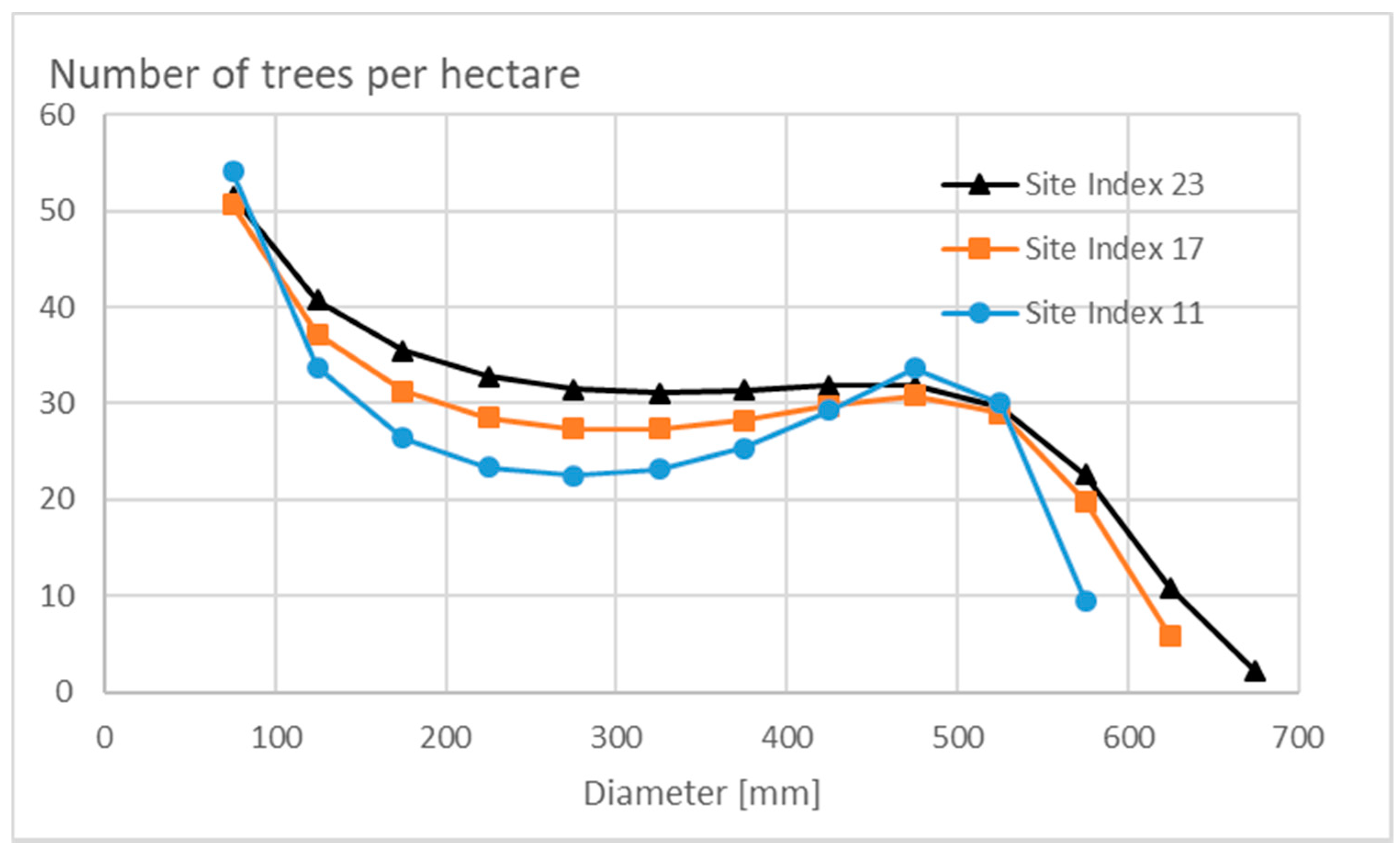
Figure 1. Number of trees in 50-mm diameter classes in the stationary state according to Equations (1)–(5) for three site fertility classes.
Sustainability 10 03662 g001
Figure 2. Commercial trunk volume in 50-mm diameter classes in the stationary state according to Equations (1)–(5) for three site fertility classes.
Sustainability 10 03662 g002
Figure 3. Commercial stumpage value in 50-mm diameter classes in the stationary state according to Equations (1)–(5) for three site fertility classes.
Sustainability 10 03662 g003
Figure 4. Commercial trunk volume harvested in diameter-limit cutting within any period of five years, including dying trees from all diameter classes, according to Equations (1)–(6) for three site fertility classes.
Sustainability 10 03662 g004
Figure 5. Commercial stumpage value of trees harvested in diameter-limit cutting within any period of five years, including dying trees from all diameter classes, according to Equations (1)–(6) for three site fertility classes.
Sustainability 10 03662 g005
Figure 6. Annualized capital return rate from diameter-limit cutting within any period of five years, including dying trees from all diameter classes, according to Equations (1)–(6) and (9) for three site fertility classes. U O c h _ n a t = 0 .
Sustainability 10 03662 g006
Figure 7. Annualized capital return rate from diameter-limit cutting within any period of five years, including dying trees from all diameter classes, according to Equations (1)–(6) and (9) for three site fertility classes. U O c h _ n a t = 0.01 .
Sustainability 10 03662 g007
Figure 8. Annualized capital return rate from diameter-limit cutting within any period of five years, including dying trees from all diameter classes, according to Equations (1)–(6) and (9) for three site fertility classes. U O c h _ n a t = 0.1 .
Sustainability 10 03662 g008
Figure 9. Annualized capital return rate from diameter-limit cutting within any period of five years, including dying trees from all diameter classes, according to Equations (1)–(6) and (9) for three site fertility classes. U O c h _ n a t = 1.0 .
Sustainability 10 03662 g009
Figure 10. Annualized capital return rate from diameter-limit cutting with limit diameters 200 and 350 mm, with 0% annual increment rate in nonoperative capitalization, according to Equations (1)–(6) and (9), as a function of capitalization ratio U O c h _ n a t .
Sustainability 10 03662 g010
Figure 11. Annualized capital return rate from diameter-limit cutting with limit diameters 200 and 350 mm, with 2% annual increment rate in nonoperative capitalization, according to Equations (1)–(6) and (9), as a function of capitalization ratio U O c h _ n a t .
Sustainability 10 03662 g011
Figure 12. Annualized capital return rate from diameter-limit cutting with limit diameters 200 and 350 mm, with 4% annual increment rate in nonoperative capitalization, according to Equations (1)–(6) and (9), as a function of capitalization ratio U O c h _ n a t .
Sustainability 10 03662 g012