Future Global Air Quality Indices under Different Socioeconomic and Climate Assumptions

Abstract

Future socioeconomic developments and climate policies will play a role in air quality improvement since greenhouse gases and air pollutant emissions are highly connected. As these interactions are complex, air quality indices are useful tools to assess the sustainability of future policies. Here, we compute new global annual air quality indices to provide insights into future global and regional air quality, allowing for the evaluation of the sustainability of climate policies. We project the future concentrations of major the air pollutants for five socioeconomic pathways covering a broad range of climate radiative forcing targets in 2100, using a fast transport chemistry emulator and the emission database produced for the sixth assessment report of the Intergovernmental Panel on Climate Change. Our findings show that climate policies are very relevant in reducing air pollution exposure by mid-century. Climate policies will have a stronger effect on the pollution reduction timing, while socioeconomic developments will have a greater impact on the absolute pollution level. A 1.5 ${}^{\circ }$C policy target may prevent all regions from exceeding the annual average limit for all pollutants considered, except PM${}_{2.5}$. We emphasize the importance of considering exposure air quality indices, when assessing sustainable policies, as being more informative rather than a population-weighted average index.

1. Introduction

The agenda 2030 [1] defines seventeen goals for sustainable development among which climate action, good health and well being, sustainable cities and life on land. Climate action and its co-benefits on air pollution relate to these goals and are crucial in defining future development policies.

The Integrated Assessment (IA) modeling community has produced in the recent decade a rich set of long-term future global scenarios. These scenarios focus mainly on global climate goals. Climate targets do not solely affect greenhouse gases levels but also air pollutants’ concentrations. The relationship between greenhouse gases mitigation and air pollution management is clear: both greenhouse gases and air pollutants are emitted by the combustion of fuels, and both influence radiative forcing. This is one of the reasons the IA community created an extensive database of air pollution pathways scenarios alongside the global mitigation scenarios [2]. This information is important not only for assessing future global climate policies but also to guide and help air pollution plans.

Air pollution has been considered the most important environmental health-related problem by the World Heath Organization in 2014 [3]. It is estimated that, in 2012, air pollution alone caused approximately seven million deaths around the world [3,4,5]. Structured and careful air pollution policies and management can help reduce this problem and avoid a significant number of premature deaths due to poor air quality.

The air pollution scenarios produced by the IA community have already provided insights into the co-benefits that come along with climate policy implementation, as for instances in [6,7]. Most of these recent scenario exercises are based on the assumption that current and planned air pollution policies will be enforced and that, until the end of the century, these policies will become gradually more stringent. However, it is only recently that the baseline scenarios also include air pollution policies, linked with the underlying story-lines and assumptions, as in the Shared Socioeconomic Pathways (SSP) scenarios [8].

The connection between climate and air pollution is significant enough to interfere with the safe achievement of the intended climate target. Climate targets are typically formulated over long time frames such as a century, while policy-makers have shorter governance cycles and are mainly concerned with short-term impacts on the population. Air pollution represents a stronger and more appealing argument than climate in the political agendas. In this context, it is crucial to understand how air pollution policies in conjunction with climate goals will play a role in locally achieving the legal air pollution objectives, more specifically the yearly air pollution limits.

In this study, we explore the SSP–RCP matrix of scenarios [2,9] to assess air quality policy implications across different socioeconomic pathways coupled with the global climate efforts to provide insights on the more sustainable policies to pursue. The SSP scenarios vary across many dimensions including Gross Domestic Product (GDP), population and urbanization [10], and other sets of assumptions, such as technological development, environmental awareness and regional fragmentation. The SSPs establish air pollution policy pathways that evolve according to a storyline which depends on the different SSP baseline assumptions.

In the SSP scenarios, air pollution controls are implemented continuously through the implementation of End Of Pipe measures. However, the stringency and the speed at which each region adopts the control measures differ across SSP scenarios. These are stylized air pollution control scenarios that represent an average bulk of measures which are consistent with each of the SSP story-lines. They go from a mere implementation of the current air pollution legislation (SSP3 and SSP4: weak scenario in

Table 1. Shared Socioeconomic Pathways (SSP) air pollution control policy levels.

SSP Scenario	Emission Factors
SSP1 and SSP5	Strong decrease
SSP2	Medium decrease
SSP3 and SSP4	Weak decrease

) to the total deployment of the best available End Of Pipe technologies for each of the sectors (SSP1 and SSP5: strong scenario in Table 1). While SSP1 (sustainability) and SSP5 (conventional development) foresee the widest and fastest deployment of air pollution controls, SSP3 (regional rivalry) and SSP4 (inequality) are the scenarios assuming the slowest implementation. The middle of the road scenario (SSP2) assumes significant advancement in pollution control, yet less than in SSP1 and SSP5. The details of the air pollution control storylines can be found in [8] and in

Table A1. Description of pollution controls in the SSPs, taken from [8].

Policy Strength	Policy Targets		Technological Innovation	SSP	Key Characteristics of SSPs
	High Income Countries	Medium and Low Income Countries
Strong	Policies over the 21st century aim at much lower pollutant levels than current targets to minimize adverse effects on population, vulnerable groups, and ecosystems.	Comparatively quick catch-up with the developed world (relative to income)	Pollution control technology costs drop substantially with control performance increasing.	SSP1 SSP5	Sustainability driven; rapid development of human capital, economic growth and technological progress; prioritized health concerns
Medium	Lower than current targets	Catch-up with the developed world at income levels lower than when OECD countries began controls (but not as quick as in the strong control case).	Continued modest technology advances.	SSP2	Middle of the road scenario
Weak	Regionally varied policies.	Trade barriers and/or institutional limitations substantially slow progress in pollution control.	Lower levels of technological advance overall.	SSP3 SSP4	Fragmentation, inequalities

. Climate policy objectives are applied to all SSPs by different integrated assessment models to cover a full range of climate radiative forcing levels, following the RCP targets [11].

Air Quality Index (AQI) serves the purpose of aggregating otherwise extensive and complex information on single or multi-pollutant concentrations. This composite characteristic of the AQI allows accounting for several factors with a single value. Typically, these indices assemble information on the most important pollutants and provide information on the level of action, generally remediative, to be carried out both by the competent authorities and by the population. Ultimately, such indicators are helpful to inform on the expected impacts of air pollution on the population. A comprehensible definition was given by Shooter and Brimblecombe [12]: “Air quality indices aim at expressing the concentration of individual pollutants on a common scale where effects, usually health effects, occur at a value that is common to all pollutants”.

Several types of AQIs have been developed, with multiple purposes and scopes. For detailed reviews of the AQIs, refer to Shooter and Brimblecombe [12] and Plaia and Ruggieri [13]. Traditionally, AQIs are used for real-time public information, but they differ in terms of the spatial aggregation method, number and type of pollutants considered, and on their time scale [14,15]. However, these AQIs have not been designed for a global and large-scale long-term assessment of air pollution risk exposure to compare global policies, especially not related to climate policy objectives and socioeconomic drivers. The CITEAIR II project [16] proposed the Yearly Average Common Air Quality Index (YACAQI), which is used to compare air quality in European cities and it is one of the most recent indices that uses annual averages. Similarly, the Energy Policy Institute at The University of Chicago has calculated the Air Quality-Life Index (AQLI) which maps the life years lost per person from ambient PM${}_{2.5}$ concentrations above a given limit, either set by local governments or by the World Heath Organization [17].

In this paper, we explore a range of global AQIs that are adaptable to the time and spatial resolution of the emissions generated by global IA models. We produce information on long-term global air pollution policy planning and annual co-benefits, instead of the more conventional approach of using AQI for real-time or near future (order of days) information. This is crucial to inform climate policy and air pollution annual strategies based on the evolution of key socioeconomic factors.

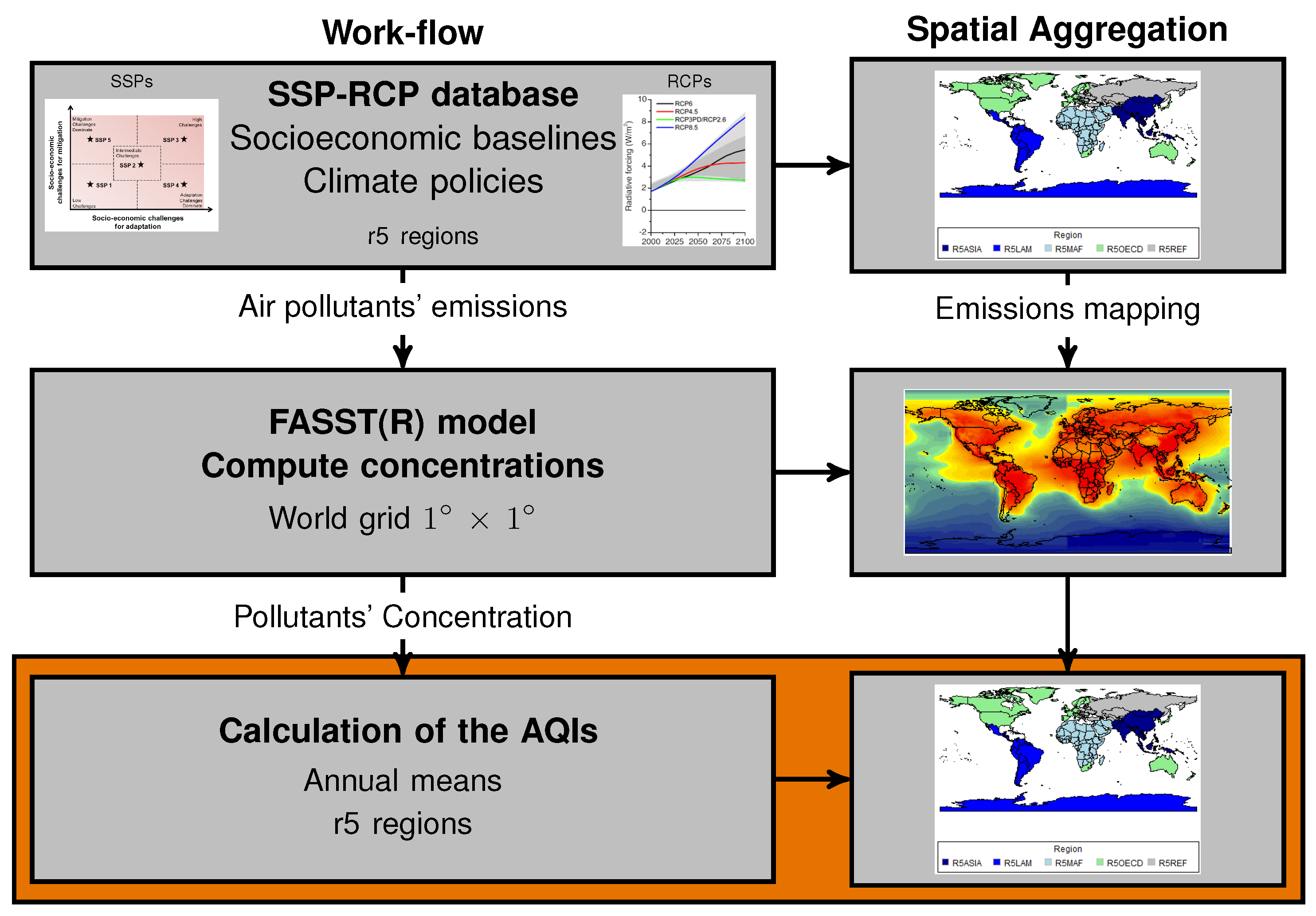
The integrated assessment models (IAMs) produce emission pathways for several pollutants, such as Sulfur dioxide (SO${}_2$), Nitrogen oxides (NO_x), Organic Carbon (OC), Black Carbon (BC), Volatile Organic Carbon (VOC), carbon monoxide (CO) and ammonia (NH${}_3$). These emissions are typically computed throughout the 21st century at 5- or 10-year time steps. The level of spatial detail is low, in the range of around 5–30 world regions. To harmonize the results across models, to allow comparability, these are often further aggregated to even larger macro-regions. Such high level of spatiotemporal aggregation poses important challenges and limitations to the design of AQI, which should be adaptable to the data provided by an IAM, include multi-pollutant information to account for air pollution synergistic effects, and at the same time must be meaningful for integrated policy decision at these spatial and temporal scales. The task of developing an AQI that provides long-term information to policy-makers is challenging. First, the future is unknown, and the projection has to be made from plausible scenarios which also contain very limited regional and temporal resolution detail. Accordingly, the AQI must be comparable amongst all regions to establish a consistent evaluation of the future air pollution pathways.

The global scope of this work does not directly provide insights into local sectoral specific policies. Rather, it contributes to positioning the local and national policies on air pollution in the context of global climate policies and the global macroeconomic development which is only possible with the help of global IAMs. In addition to the computed AQIs themselves, it provides a framework for air quality indices calculation for long-term integrated policies, which rely on aggregated information (indices) to evaluate the sustainability of multi-objective policies or co-benefits.

The aim of this paper is to provide a regional evaluation at the global level of future air quality based on a range of different socioeconomic scenarios framed in the context of global climate change policy. This work attempts to provide information to assist policy-makers with the design of their policies when negotiating climate goals and commitment strategies. We provide information on the accomplishment of future regional air pollution goals as a co-benefit of climate policies and socioeconomic development. This will help to understand the importance of air pollution in the context of global climate policies. The AQIs are strongly dependent on their underlying assumptions, such as mathematical formulation and the definition of the harmful thresholds. Therefore, we do not rely on a single AQI, but we analyze a range of possible AQIs and discuss their meaning and pertinence for policy making at this scale. We set out to assess the consequences in terms of future air quality around the world based on the most recent scenario exercise for the IPCC’s next assessment report, namely the SSP–RCP scenario matrix [2]. The pollutant pathways are provided by the SSP database and represent a range of socioeconomic scenarios each with a corresponding air pollution emissions storyline coupled with climate targets represented by the RCPs (Representative Concentration Pathways), which establish radiative forcing targets. This is to our knowledge the first attempt to assess multi-pollutant future air pollution, through the use of AQIs, based on different scenarios of socioeconomic assumptions and climate targets.

In the Results section we present the results of the several AQI across the SSP–RCP scenario matrix. First, we present the global population average indicator (Global Yearly Average Air Quality Index, GYAQI) for all the macro regions and we discuss the regional variations. Secondly, we show possible variations of this index to overcome the multi-pollutant averaging issues. Furthermore, we introduce the exposure indices and explain how they vary across the different types of policies. Finally, we discuss in more detail the regional exposure results. The Methods section includes the design of the AQIs and the framework for the calculation of the results. Finally, we draw the conclusions.

2. Results and Discussion

This section provides a qualitative assessment of the new global and regional AQIs under the different socioeconomic developments and climate scenarios. All the results can be browsed in an interactive on-line tool hosted at Supplementary Materials https://datashowb.shinyapps.io/AQIvis.

2.1. The GYAQI under Different Socioeconomic Developments

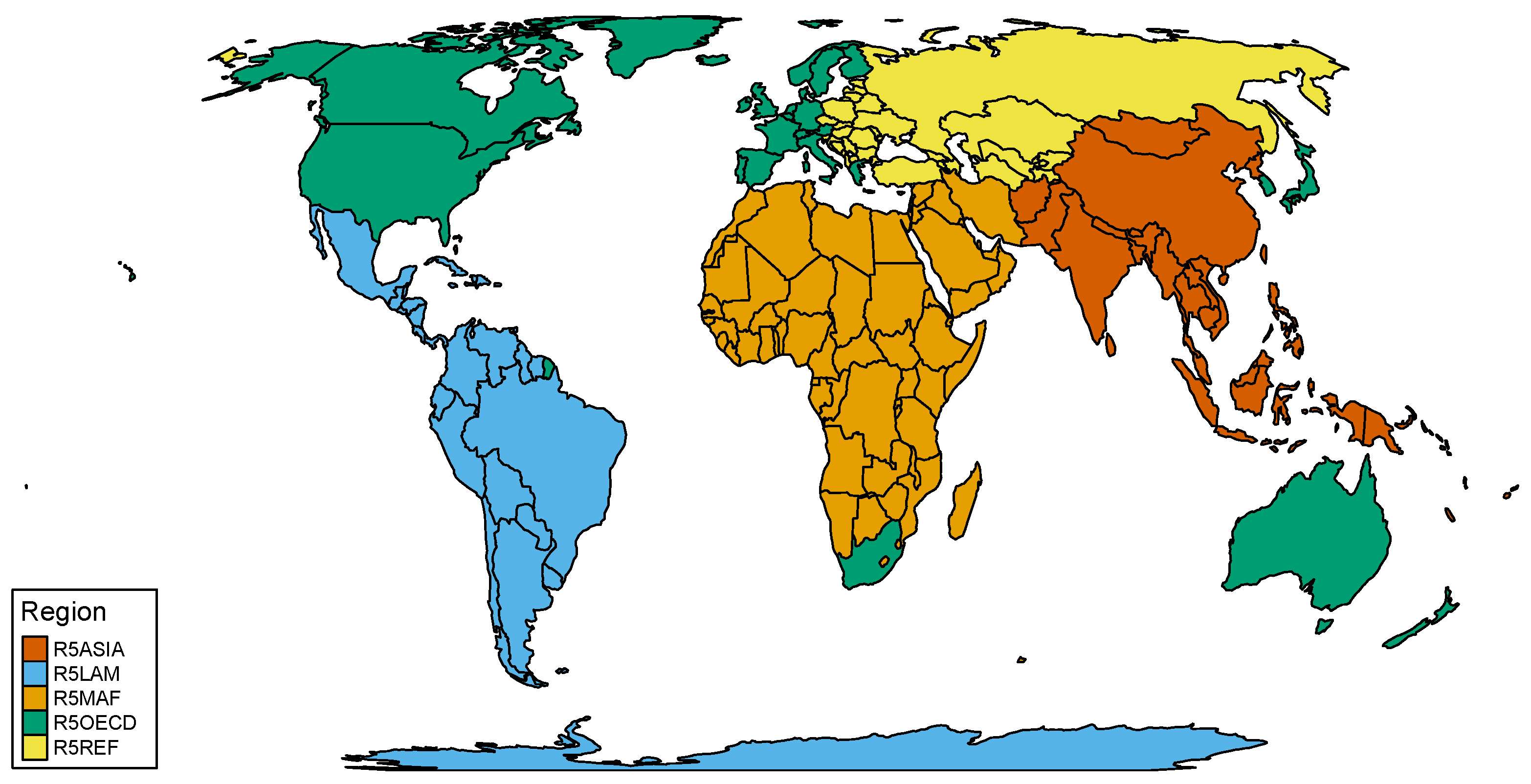
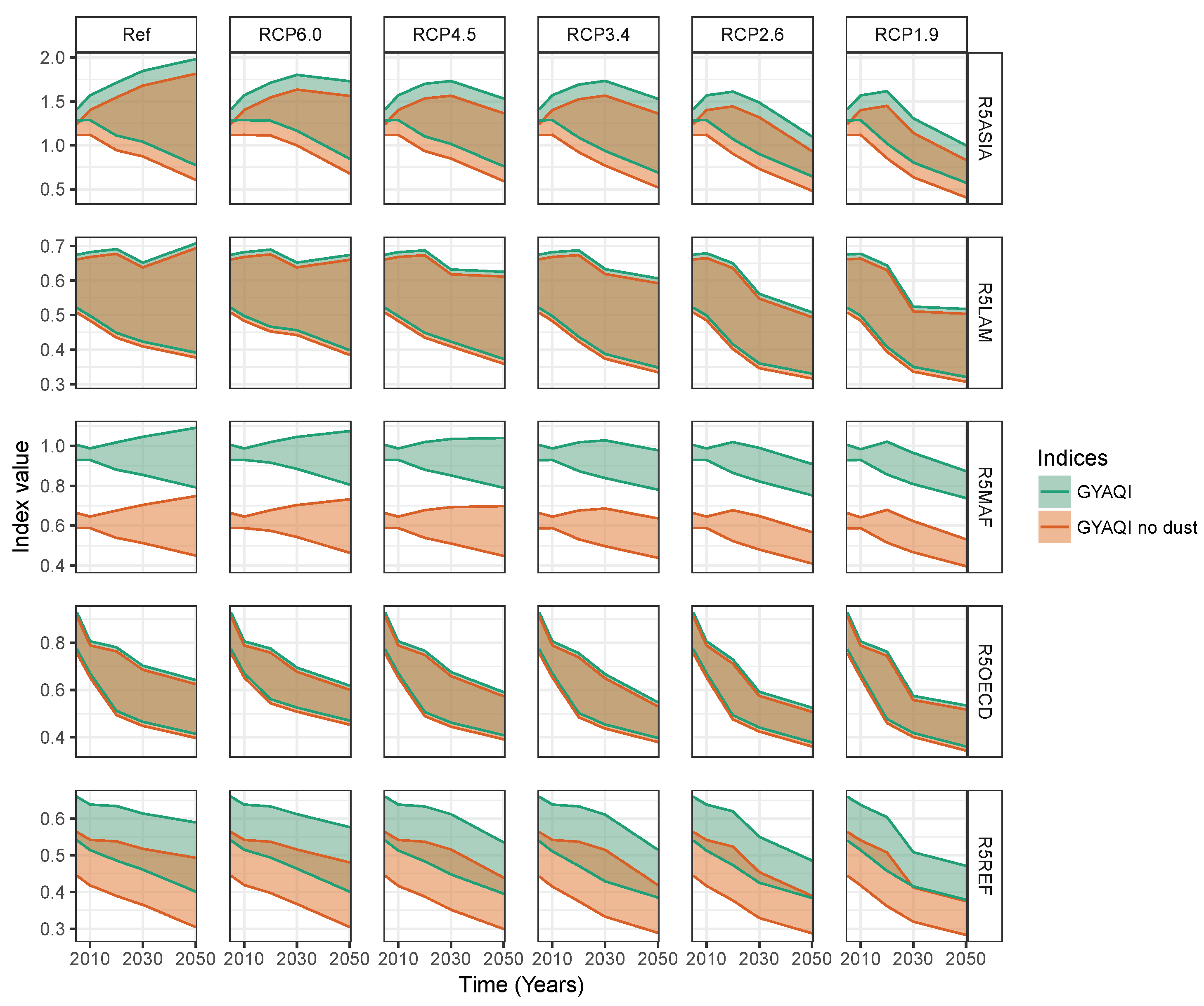
Considering the reference scenario (“Ref”) in Figure 1, where no climate policy is considered, one region excels as a real future challenge for air pollution legislation compliance, the region of Asia. This challenge is even more evident in SSP3, SSP4 and SSP2, with the GYAQI showing values above one throughout the whole second half of the century. The SSP3 (regional rivalry) scenario shows an increasing trend with time only inverted by climate policy, however keeping the values above the limits. The poor air quality in Asia is coming from the fossil fuel supply which is expected to grow in all the SSP baselines, contrary to the OECD region where oil supply will flatten or decrease. This combined with the mild air quality policies of SSP3 leads to poor air quality. Asia has the highest oil and coal primary energy production, and biomass supply is generally foreseen to rise more in Asia than in others regions. In this case, the air pollution controls foreseen in SSP3 are not enough to keep the GYAQI levels in Asia to the composite limit levels. Energy use will also be key to bend the trend curve of the GYAQI towards a decreasing trajectory after 2030, as explained by the difference between SSP3 and SSP4, which both assume the same air quality policies but differ on the energy demand and supply side. Climate policies, as seen by the stringency of the RCP targets, will be key to lower pollution as we observe that as the climate targets tighten the GYAQI approaches the value one. However, only the climate target set by the Paris agreement (RCP1.9, which corresponds to 1.5 ${}^{\circ }$C) prevents the GYAQI, independently of the socioeconomic assumptions, from assuming values above one by the middle of the century.

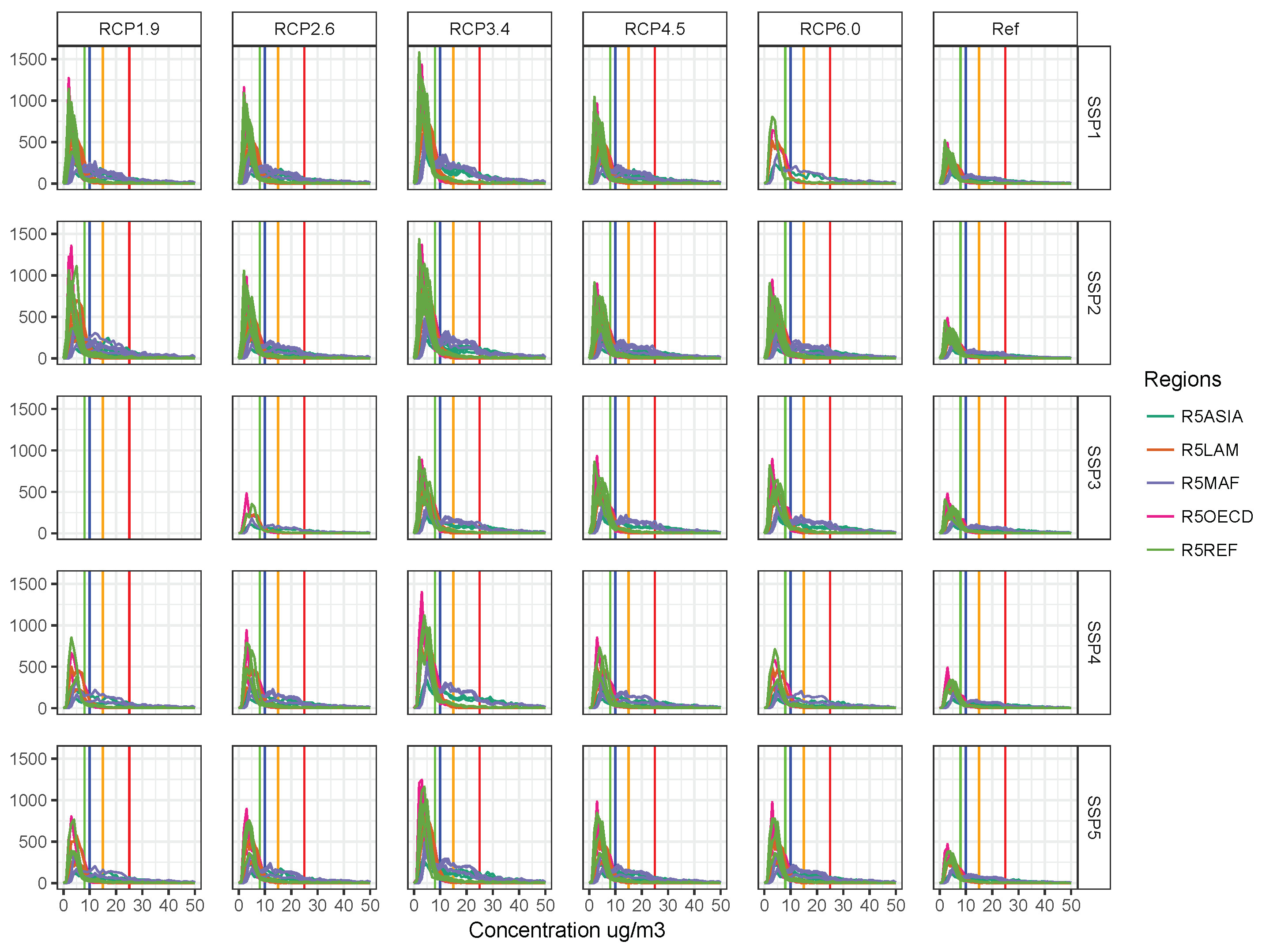
The Middle East and African region have a GYAQI that is generally dangerously close to one, and in the case of SSP3 combined with no climate policy or mild climate polices, it will exceed the composite limit. In this case the PM${}_{2.5}$ sub-index is responsible for the higher values of the composite index. It is important to note that PM${}_{2.5}$ in Middle East and Africa is strongly driven by the natural dust, which is one of the reasons the trend does not undergo drastic decreases even for very stringent policies (Figure A8). The other reason is that the ozone sub-index trends have a flat behaviour around the value one.

For both regions, Asia and Middle East and Africa, unlocking international climate agreements are crucial to bring air pollution levels less harmful levels. When negotiating climate targets these regions would benefit from a global optimal emission pathway to lower their national air pollution.

Other regions do not present exceedances to the defined composite standard limits when analyzing the GYAQI, for all the SSP–RCP combinations. In OECD, we observe a general constant decrease on the GYAQI until 2050. The Latin American (LAM) and the reforming economies (REF) regions also see a decrease, although smoother.

The GYAQI is a multi-pollutant index that averages all the pollutants with equal weights. However, this could potentially be problematic, since it might hide pollutant-specific problems. To overcome come this drawback, we look at the pollutant sub-indices (${\psi }_p$) and the variant of GYAQI, namely GYAQIv, which focuses on the two most problematic pollutants, fine particulate matter and ozone.

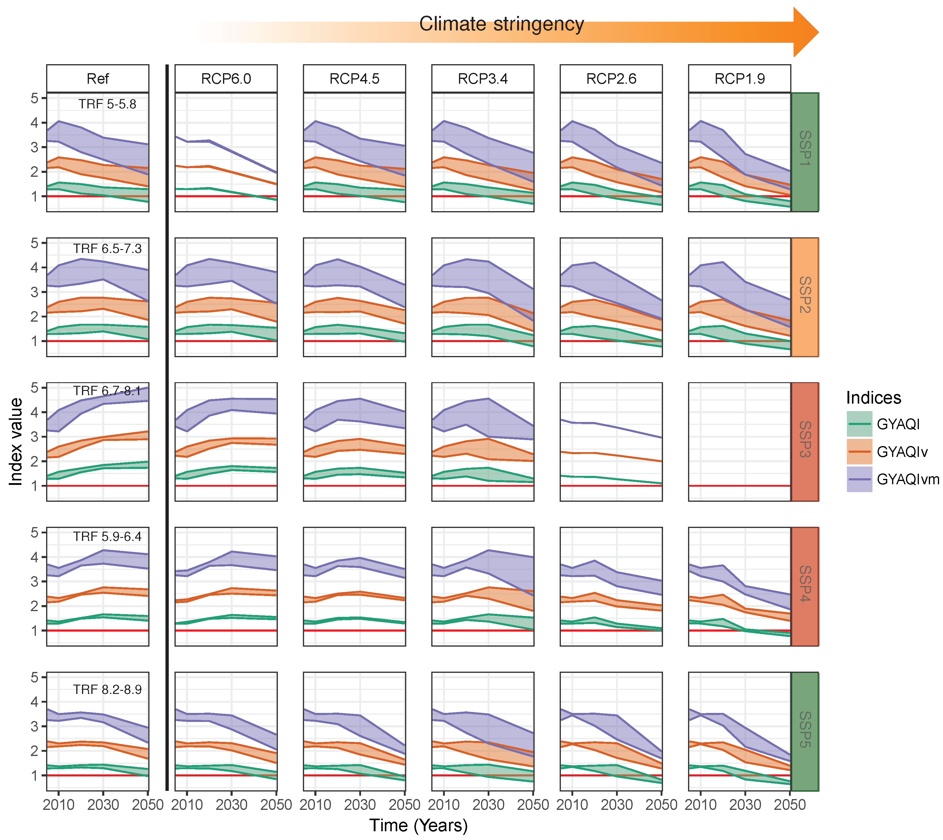
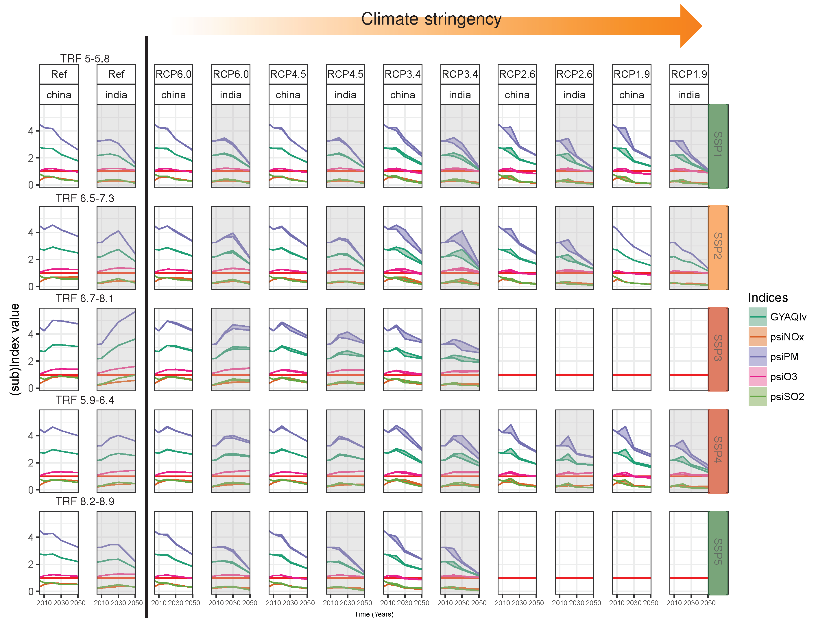
Figure 2 shows the sub-indices ${\psi }_p$ and the GYAQIv index for Asia. The GYAQIvm, which takes the maximum sub-index instead of the average, is given by the highest ${\psi }_p$ in the figure. The sub-indices results show that PM${}_{2.5}$ and ozone are the most problematic pollutants in Asia, being almost constantly above the limits. Neither the climate policies nor the air pollution controls would be enough to avoid PM${}_{2.5}$ exceedances, the best outcome is found for SSP1 (Sustainability) and the most stringent climate policies, however, the value is still above the limit. SSP5 (fossil-fuel development) also shows similar results but the lower bound of $\psi$_PM2.5 in SSP1 is lower. Note that the narrower ranges of the SSP5 scenario are not necessarily due to less model uncertainty, but rather to the lower number of models implementing this scenario. When comparing SSPs, the SSP1 still turns out to be the scenario that offers the largest possible air quality improvement, with its lower bounds being lower than in SSP5, for all RCP targets, except RCP6.0, and all regions. The ozone sub-index varies in a narrower range (0.8–1.4), the Paris agreement climate target (RCP1.9) assures that ozone will respect the defined limit under all the socioeconomic assumptions by 2050. However, the most stringent air pollution controls and most sustainable socioeconomic assumptions (SSP1) might also be enough to keep ozone under the limit by 2050, as the lower bound of SSP1-Ref is lower than one.

The detailed analysis of the sub-indices reveals that the region of Middle East and Africa will also experience air pollution problems, mainly coming from ozone, which has, similarly to Asia, a very flat profile (${\psi }_{O3}$ of 0.9–12) revealing the difficulties in tackling this pollutant. Ozone is a secondary pollutant, i.e., its concentration depends on other pollutants and meteorology in a non-linear relationship, making ozone-targeted policies is more complicated.

Figure 2 also highlights the importance of considering indices that are multi-pollutant composites but are less dependent on averages. The GYAQIv and GYAQIvm (graphically given by the highest sub-index) reveal that air pollution problems still persist by 2050 even if, in general, the air quality improves. The study of the pollutant’s sub-indices shows high adequacy of AQIs which are less sensitive to averages. Both GYAQIv and GYAQIvm exhibit the air pollution problems that were otherwise hidden due to the low values of NO_x and SO${}_2$ (see Figure A2).

Undoubtedly, the air pollution emissions pathways induced by socioeconomic development will be important to improve regional air quality. This is translated by the lower limit bound of the more stringent climate scenarios and also by the narrowing of the model range (Figure 2). However, these levels are not enough to be considered as safe and the climate policies will play a more crucial role, in particular in the mid-century, which is consistent with previous studies [7]. This is especially important for PM${}_{2.5}$ pollution which is one of the most worrisome pollutants in terms of human health impacts. All models agree that, from 2030 to 2050, in all SSPs, an RCP1.9 climate policy, consistent with 1.5 ${}^{\circ }$C degrees, would prevent all regions of the world from exceeding the annual population-weighted average limit for all the pollutants, except PM${}_{2.5}$.

2.2. AQIs and Climate Policies

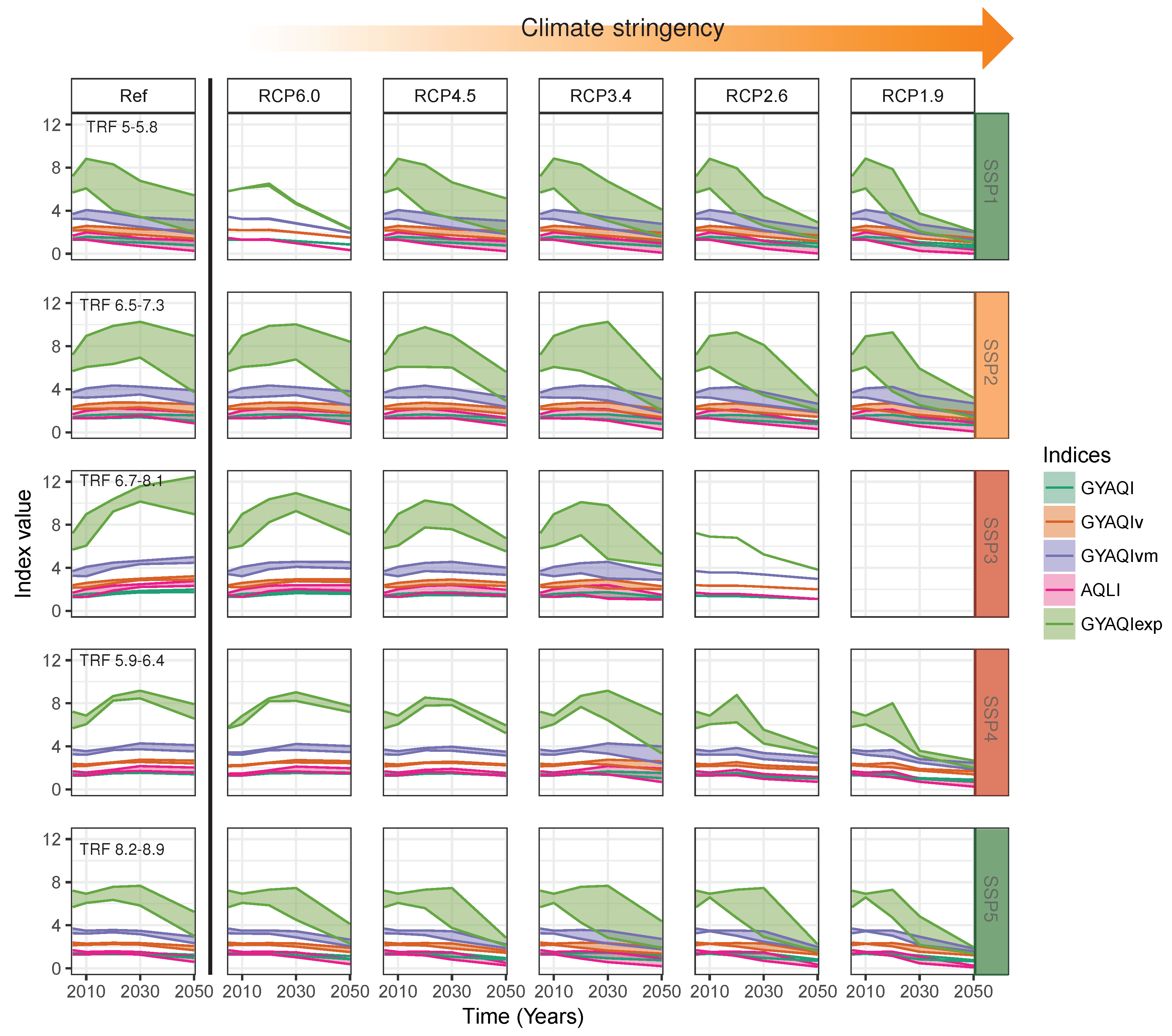
The pollutant-specific indices bring clarity to the results of the multi-pollutant AQIs. However, they do not inform the policy-makers on whether large parts of the population are exposed to high levels of pollution. Figure 3 shows the AQIs results for Asia where more pollution problems are expected to arise (see population exposure in Figure A3).

Exposure indicators, the GYAQIexp and the AQLI, are more responsive as both the concentrations and fractions of exposed population vary. The GYAQIexp penalizes high levels of exposure and the AQLI measures the years lost due to non-compliance of the limits. In Asia, GYAQIexp never equals GYAQI (i.e., there is always a fraction of the population exposed to at least the double of the limit values) independently of the socioeconomic conditions and the climate policies.

Air pollution policies seem to play a more crucial role in reducing the exposure AQIs than when considering the non-exposure AQIs. This is also observed in

Table 2. The median [minimum–maximum] AQLI index range across models and SSPs, in 2030, expressed in years of life saved if the air quality limit was met.

Region	Climate Targets
	Ref	RCP6.0	RCP4.5	RCP3.4	RCP2.6	RCP1.9
ASIA	2.2 [1.3–3.0]	2.2 [1.5–2.9]	2.0 [1.2–2.9]	2.0 [1.1–2.9]	1.6 [1.0–2.2]	1.3 [0.8–2.0]
LAM	0.2 [0.1–0.4]	0.2 [0.1–0.4]	0.2 [0.1–0.4]	0.1 [0.0–0.4]	0.1 [0.0–0.3]	0.1 [0.0–0.2]
MAF	1.3 [1.1–1.5]	1.3 [1.2–2.5]	1.3 [1.1–1.5]	1.3 [1.1–1.5]	1.2 [1.0–1.3]	1.1 [1.0–1.3]
OECD	0.2 [0.1–0.3]	0.2 [0.1–0.3]	0.2 [0.1–0.3]	0.2 [0.0–0.2]	0.1 [0.0–0.2]	0.1 [0.0–0.2]
REF	0.2 [0.2–0.3]	0.2 [0.2–0.3]	0.2 [0.2–0.3]	0.2 [0.2–0.3]	0.2 [0.1–0.2]	0.2 [0.1–0.2]

, where the range of the medians across RCPs is lower than the minimum to maximum range within each RCP. Similar to before, the best air quality is seen when both stringent climate policies and SSP1 or SSP5 are enforced.

This can be seen looking at the GYAQIexp, reaching values close to the GYAQI, and the lower bounds of the AQLI achieving values under one year of life lost by 2050. The results of the AQLI found for the beginning of the century are compatible with the ones found in [17], although the limit is not the same. SSP1 achieves lower levels of premature years lost with milder climate policies as the lower bounds of the AQLI levels are the lowest compared with the other socioeconomic scenarios. On the other hand, SSP3 foresees more than two years of life lost in Asia by 2050 for all climate targets, and more than three years of life lost in the case of SSP3-Ref. Climate policies will help in SSP3 to reduce the AQLI to around one or more years lost after 2030 with RCP4.5 and more stringent, still unfolding important values of the exposure AQIs. In general, the climate policies will not impact so much on the magnitude of the AQLI value but will mainly increase the speed at which those levels are achieved.

The GYAQIexp shows a broader range of values, as there are many levels of penalty depending on the magnitude of the exceedance. The “Ref” scenario shows that SSP3 and SSP4 alone expose significant fractions of the population to high levels with GYAQIexp always significantly above the GYAQI. Again, the socioeconomic assumptions of SSP4 are more favourable than in SSP3, as we observe a decreasing trend after 2030 in SSP4 even without climate policies. In the other SSPs, the lower bound is closer to the GYAQI level in 2050, meaning that air pollution policies reduce exposure, however only after 2030, with the exception of SSP1 and SSP2, where the decreasing trend of the GYAQIexp starts earlier.

The impact of climate policies becomes more important after 2030, where both the range of the GYAQIexp narrows and the values decrease to levels closer to the GYAQI, although still very high in the Asian region. Similar to the “Ref” case, SSP3 and SSP4 show high values of the GYAQIexp which remains substantially high even with the most stringent climate policy. The SSP3 is incompatible with RCP1.9 and RCP2.6 (only one model solved SSP3–RCP2.6) indicating that this combination is unlikely to happen. However, the only result available shows that the air pollution problem in Asia would most probably be left unsolved in the case of GYAQIexp. In SSP5, the decrease provoked by the climate policies is slower than in SSP1, although the lower bounds show a faster decrease than in SSP2 where some models predict important air pollution exposure levels even with very stringent climate policies. The analysis of the exposure indices shows that climate policies do not lead to good air quality, even if they help to reduce significantly exposure by the mid-century, there will be populations exposed to very high levels of pollution. Under these climate stringent policies, not only coal and oil supply are significantly reduced, but also the gas production leading to lower air pollution levels.

The regions that struggle more with pollution problems have much to benefit from a global climate policy. Climate change is a global problem, thus mitigating GHG can be carried out where the marginal abatement costs are lower worldwide, which means that cost-efficient international efforts will lead to investments in the regions that most need air pollution reductions due to lower abatement costs. This will be important for regions such as Asia, especially in India, reducing greatly the air pollution exposure.

2.3. The Regional Multi-Pollution Challenge

2.3.1. Asia

In Asia (Figure 2 and Figure 3), air pollution is driven mainly by PM${}_{2.5}$ and ozone. SO${}_2$ and NO_x show values constantly under the defined standard limits, with nitrogen oxides showing a flatter profile over time, only increasing regularly in SSP3 under very mild climate policies leading to high emissions in the industrial and transport sector. SO${}_2$ shows a decreasing trend for all scenarios, except in SSP3 in the Reference scenario. The implementation of air pollution controls enforced in the other SSPs provokes the decrease and, in the case of SSP3, the climate policies restrict the coal use as they become more stringent.

Ozone remains one of the most problematic pollutants: all models foresee exceedances until 2030. Only SSP1 and SSP5 air pollution controls and socioeconomic assumptions show a decreasing trend in the absence of climate policies. For ozone, climate policies are more important than socioeconomic development. However, they are not as effective in bringing down the ozone concentrations as compared with other pollutants.

It is the ensemble of both climate and socioeconomic “greener” scenarios SSP1/2–RCP1.9, that assures, for all models, no exceedances of seasonal ozone limits by 2050. The SSP3 scenario always unfolds a world where ozone is above the standards in Asia. In SSP1, the lower limits of the model range prove possible to be below the limits even with no climate policy in Asia. The PM${}_{2.5}$ sub-index shows a behaviour similar to that of ozone. Asian back carbon emissions, especially in the transport and industry sectors, are the highest amongst the world regions, except in the power sector where they follow a pattern similar to that of the OECD region.

Analyzing the fractions of the population above the standard PM${}_{2.5}$ levels (Figure A3) shows that the SSP3 socioeconomic assumptions are the most damaging regarding pollution exposure where we observe significant fractions of the population (more than $3/4$) exposed to PM${}_{2.5}$ levels twice the limits and more than half of the population exposed to values three times higher than the threshold. Climate policies are effective in decreasing the endangered fraction of the population, especially to avoid exposures above twice the limit and especially after 2030.

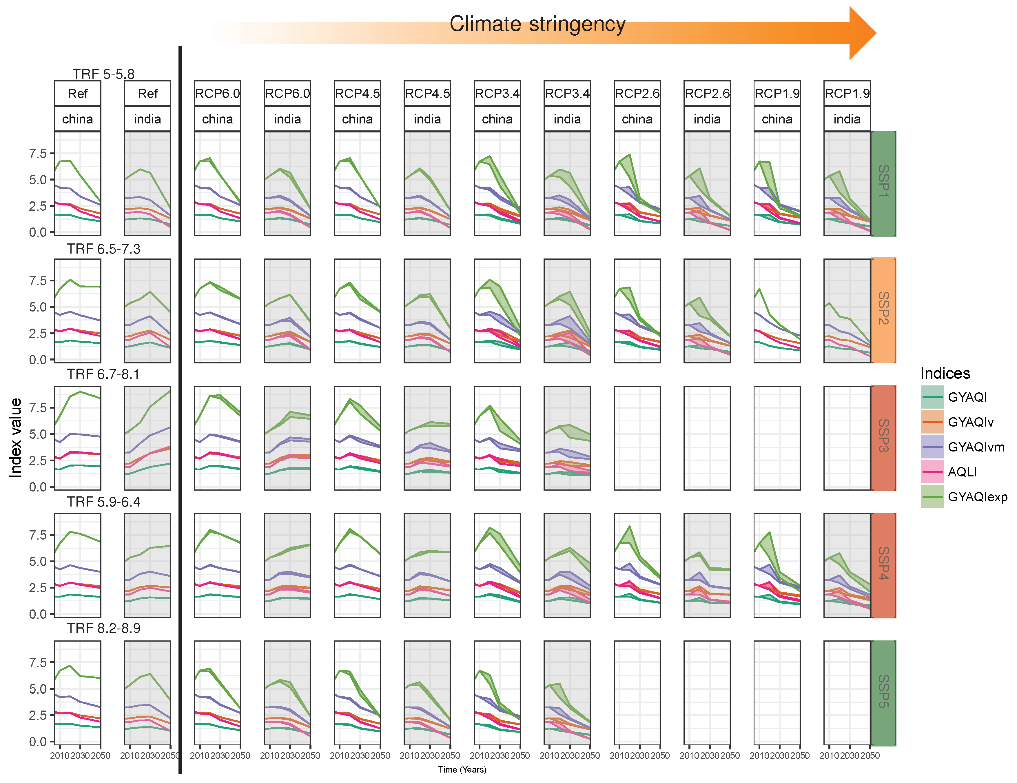
Asia is a major macro-region that includes two of the major polluting countries in the world, China and India. The recent commitments of the Paris agreement and the enforcement of the national air pollution plans show two different ambitions what concerns both air pollution and climate goals. To study this in a greater detail, we analyze the results of the SSP–RCP scenario exercise of the model WITCH-GLOBIOM that includes these two countries separately. Figure 4 and Figure A7 show the indices and the sub-indices for these countries. The exposure index GYAQIexp shows higher values than the macro-region results, because in both India and China the fractions of exposed population to extremely high values (i.e., $\alpha >5$) is zero, whereas in the whole macro-region of Asia there are exposures to extremely high values. On the other hand, India shows lower values than the Asia region. The most interesting aspect is the difference in trends. Looking at SSP3 and SSP4, when no climate policy is in place, one observes that China peaks its AQIs earlier than India and inverts the trend of the exposure indicator (GYAQIexp), whereas in India in SSP3 this trend does not invert and the AQIs values keep increasing over time. The air pollution controls and socioeconomic assumptions of SSP2, SSP3 and SSP4 are more important in India than in China where the intensive economic growth will maintain the AQI levels high even if with a decreasing trend towards the middle of the century. Climate policy in India will act faster than in China, but this is not surprising since decarbonization is happening first in India where the marginal abatement cost is lower.

2.3.2. Latin America

In the Latin America region, the indices show good scores indicating that the annual averaged air quality limits will probably be respected. The levels of ozone, PM${}_{2.5}$, SO${}_2$ and NO_x will remain under the limits. All the pollutants show decreasing trends, except PM${}_{2.5}$ which stays flat from 2030 to 2050 in SSP2 and SSP3. Despite that, half of the population will remain above the PM${}_{2.5}$ limit values, although extreme exposure will most probably not take place especially after 2030, with the exception of SSP3. A slight rebound increase at the end of the half century in SSP2 is observed and remain constant throughout time in SSP3. In SSP3, emissions increase and remain high in the industry and transport sectors due to continuous general high gas and oil supply even with climate policies in Latin America. Latin America shows one of the lowest AQLI (Table 2), with few months of life lost due to PM${}_{2.5}$ by 2030.

2.3.3. Middle East and Africa

The prominent challenge for the Middle East and Africa region regarding air pollution is ozone and PM${}_{2.5}$. In all scenario combinations, there is always a chance that ozone will exceed the season limit at some point in time, especially until 2030. Ozone itself is known to have important impacts on human health [18].

In the case of SSP1, RCP3.4, or stringier, is enough to keep average ozone levels within limits by 2050. However, in SSP2, SSP4 and SSP5, only the most stringent climate policies will deliver good results. SSP3 will always deal with ozone exceedances independently of the climate policy, most probably due to the VOC emissions from the power and residential sectors which are the highest in the world. The wide use of oil and biomass at levels compared to OECD and Asia in the Middle East and Africa regions and the lower level of deployment of air pollution controls contribute to the high VOC emissions observed. Additionally, emissions from solvent use tend to increase over time and grassland burning emissions are very high in this region. These emissions are exogenous in most of the IAMs and they are therefore not reactive to climate policies.

In this region, people are very exposed and the vegetation might suffer high losses. Although the aggregate air quality index shows general compliance, the exposure indices show that important parts of the population will be exposed to values above the limit.

NO_x and SO${}_2$ have values well below the limits. PM${}_{2.5}$ shows high values and the AQLI is around 1.2 in all SSP–RCP combinations (Table 2), with half of the population being exposed to concentrations twice the annual limits until 2030.

In what concerns PM${}_{2.5}$, it must be noticed that in this region a big share of this pollutant concentration comes from natural dust, as seen in Figure A8. This impacts not only the PM${}_{2.5}$ but also the composite indices. In the case of Middle East and Africa, the natural dust impact is very significant, and similar results are found in [8].

2.3.4. OECD Countries

OECD is the region where the most efficient air pollution control policies are deployed in all SSPs. In what concerns the PM${}_{2.5}$ exposure, low fractions of the population are exposed above very high limits. However, even with the very fast improvements by 2030 in any SSPs, about 25–50% of the total OECD population will be above the limit unless climate policies enter into force. In SSP1, the high exposures to PM${}_{2.5}$ are substantially reduced by 2050, without the help of climate policies. The estimated years of life lost due to PM${}_{2.5}$ exposure is of 0.17 years, in general (Table 2).

Ozone is the other potential problem in the OECD region, remaining stable and dangerously close, but always below, the limit with soft improvements until 2050. As in the Middle East and Africa region, the VOC emissions in the power sector, due to the high supply of oil and biomass, and to some extent in solvent use might be responsible for the high ozone levels. Climate policies seem to play a marginal role in the case of ozone in OECD. On the other hand, it is the socioeconomic assumptions that will be determinant for ozone pollution in OECD, where SSP1 is enough to push down ozone concentrations even if not significantly, mainly due to the VOC emissions reductions in the industry and transport sectors. Similar to the other regions, both SO${}_2$ and NO_x seem to be safely under the defined limits, with decreasing patterns in all the SSP–RCP combinations.

We analyze the specific results for the WITCH-GLOBIOM native regions within the OECD macro-region, USA, and Europe (divided into old and new Europe, where old represents the member of the European Union (EU) and new the non-EU members), shown in Figure A9. As for the OECD region, we observe a steep decreasing trend in all the AQIs starting already in the first years of the century. However, within the OECD, we observe regional differences in the magnitude of the AQIs, with the non-EU members being above the OECD values, the EU members being under and the USA following closely with the OECD macro-region. The most problematic pollutant is PM${}_{2.5}$ in non-EU members: its sub-index remains above the limit in these countries even SSP1–RCP1.9. All the pollutants sub-indices in EU are under the limits. However, even if the population weighted average indicates no problems, there will still be fractions of the population exposed to levels above the limit as seen by the exposure indices. The USA follows a path similar to that of the EU-members, dealing only with PM${}_{2.5}$ exceedances at the very beginning of the century.

2.3.5. Reforming Economies of Eastern Europe and the Former Soviet Union

The Reforming Economies of Eastern Europe and the Former Soviet Union region is one of the regions where there is less uncertainty across models. Ozone, as in all the other regions, remains close to the limit. The power and residential sector NO_x emissions are probably the main drivers of ozone. SO${}_2$ and NO_x are well below the limits. This region shows low AQLI index across all SSPs and RCPs, the fraction of exposed population is low and decreases sharply over time even with the most adverse socioeconomic drivers and without the help of climate policies. The PM${}_{2.5}$ concentrations in this region are largely affected by the natural dust (Figure A8), in all scenarios, PM${}_{2.5}$ exposure decreases sharply over time, even if around 25% of the population will still be exposed to levels above the limit. Air pollution policies as taken into consideration in the different SSPs, seem more effective in all the pollutants sub-indices with respect to climate policies.

3. Methods

3.1. Air Pollution Emission Pathways

We used the SSP database (available at https://secure.iiasa.ac.at/web-apps/ene/SspDb/dsd), which contains air pollutant emissions of the combined SSPs and RCPs targets resulting from the assessment of several Integrated Assessment Models (IAMs). The air pollutants emissions in these scenarios might vary due to two drivers: (i) the emission factor storyline, which depends only on the SSP baseline; and (ii) the energy activities which are both dependent on the SSP baseline assumptions and on the constraints imposed by a given climate policy (i.e., radiative forcing target, or the RCP dimension). Air pollutant Emissions were provided for five highly aggregated regions, defined as OECD (includes the OECD 90 and EU member states and candidates), REF (Reforming Economies of Eastern Europe and the Former Soviet Union), ASIA (includes most Asian countries with the exception of the Middle East, Japan and Former Soviet Union states), MAF (this region includes the countries of the Middle East and Africa) and LAM (this region includes the countries of Latin America and the Caribbean) [19]. The regional geographical mapping is shown in Figure A1. Although IAMs native regional data are not publicly available in the SSP–RCP database, we have calculated the AQIs for the native regions of the WITCH-GLOBIOM model to provide more insight into the intra-regional variations that these policies imply. We focus on the Chinese and Indian pathways within the Asiatic region and the European and north American indicators within the OECD region.

The air pollutant emissions from the SSP database are generated by IAMs, which result from the cost-efficient greenhouse gases emission trajectories that comply with a climate (radiative forcing) target. IAMs are not forecasting models, they generate the emission pathways according to the SSP narratives. They also provide the emission sources, i.e., the technologies and fuel mixes, given a set of plausible assumptions, constraints and emission factors [7]. The climate targets are a constraint to the IAMs which then optimize the investments across regions and sectors to achieve the climate targets. This means that, even given the model harmonized assumptions established in the SSP narratives, for the same climate policy (radiative target), each model yields different optimal pathways, depending on their optimization methods, on their regional and sectoral resolution, and on their cost and efficiency assumptions. The multi-model results provide a richer estimation of the possible futures, allowing to account for uncertainty, which is crucial for long term decision making.

We included the results from the six participating integrated assessment models, namely, AIM/ CGE [20], GCAM [21], IMAGE [22], MESSAGE-GLOBIOM [23], REMIND-MAGPIE [24] and WITCH-GLOBIOM [25], which provide air pollutants emissions. These models are well established and have participated in the IPCC report assessments [26], with many published literature [2,11]. We considered the scenarios for all SSPs and all climate targets, providing an increasingly stringent climate target defined as the total radiative forcing in 2100. Note that not all the models run all the combinations of SSP–RCP scenarios. The SSP database is the first large-scale scenario exercise producing a large number of consistent outcomes concerning economic, energy, emissions, and climate variables. It is the next scenario generation for the climate policy community informing the international climate negotiations.

3.2. Air Pollution Transport Model

We used a fast chemistry transport model, FASST(R), an R version of the reduced-form TM5-FASST model developed at JRC-Ispra, to compute the annual concentrations of several pollutants p, namely SO${}_2$, NO_x, fine Particulate Matter (PM${}_{2.5}$) and O${}_3$. TM5-FASST is a source-receptor reduced form model of TM5 full chemical transport model [27].

The fine PM${}_{2.5}$ include Particulate Organic Matter (POM), secondary inorganic PM, dust and sea-salt. The FASST(R) model produces concentrations on a world spatial grid of resolution of 1${}^{\circ }\times 1^{\circ }$. The FASST model has already been previously used in other studies to assess premature death from air pollution exposure [7]. It includes an urban increment algorithm to account for the population distribution and the distribution of PM concentrations [28]. The FASST model full validation against TM5 can be found in Van Dingenen et al. [29] and more informally in Leitao et al. [28]. According to these studies, FASST performs well in comparison with the full chemical transport model TM5 and its reduced form does not compromise the output validity.

The macro-regions emissions are pre-processed in order to obtain world gridded emissions using the Global Energy Assessment [30] as a proxy to disaggregate emissions spatially, as in Leitao et al. [28].

Figure 5 presents a schematic representation of the workflow for the calculation of the AQIs.

3.3. The Air Quality Indices (AQIs)

3.3.1. The GYAQI (Global Yearly Air Quality Index)

We built on the YACAQI (Yearly Average Common Air Quality Index), based on yearly averages, as proposed by the CITEAIR II project [16]. The YACAQI helps policy-makers to orient and design their local air pollution policies to prevent the air quality levels from exceeding the legal standards. These are concentration values above which air pollution is considered to have a negative impact on human health. Although the aggregated nature of an index summarizes the information in a single value, the relationship of the index with human health impacts remains [31]. We keep the focus on the most relevant pollutants and on the annual mean concentrations from the IAM emissions pathways. While additional pollutants are harming human health, such as polycyclic aromatic hydrocarbons, mercury, lead, benzene and even dioxins, the concentrations of these pollutants are usually correlated with the concentrations of the main pollutants considered in this study [32,33].

The GYAQI is formulated using the same principle of “difference to target” of the YACAQI, but we adjusted the reference concentration limits and the pollutant species to the IAM output, as shown in

Table 3. The GYAQI assumptions, assuming the most stringent annual air quality limit, as described in [34].

Pollutant	Limit Value	Metric
NOx	yearly average 30 NO${}_2$ $\mathsf{\mu }$g/m${}^3$	yearly average $C_{N{O}_x,t,r}$
PM${}_{2.5}$	yearly average 8 $\mathsf{\mu }$g/m${}^3$	yearly average $C_{P{M}_{2.5},t,r}$
O${}_3$	Summer months average 120 $\mathsf{\mu }$g/m${}^3$	M3M ${}^a$ $C_{O_3,t,r}$
SO${}_2$	yearly average 20 $\mathsf{\mu }$g/m${}^3$	yearly average $C_{S{O}_2,t,r}$

${}^a$ M3M represents the maximal three-month mean of daily maximal hourly ozone [35].

. The limit values are defined as annual, or seasonal for ozone, and correspond to the most stringent standards per pollutant to aim at the most restrictive air quality policy. The definition of the annual threshold value is not consensual and there is a range of values considered across regions and institutions [34]. A summary of the annual air quality limits for the different pollutants across regions can be found in Gulia et al. [34]. To address the fact that the AQIs strongly depend on the established limit (as shown in Figure A4), we use the lowest limit, so that the results can be thought of informing a “no regret” decision.

It should be mentioned that exposure metrics, on which the epidemiological studies are based, are in fact annual (PM${}_{2.5}$) or seasonal (O${}_3$) means observed at (urban and regional) background monitoring stations, and the resulting relative risk implicitly includes the local peak exposure of the population. Ozone is the only pollutant for which a seasonal metric has been used instead of the annual average. M3M is the metric used in the Global Burden of Disease study to evaluate mortalities from long-term exposure [36]. It is used as a health metric that accounts for high pollution hourly episodes and can be more directly associated with human mortality [29]. This metric is more robust when it comes to long term air quality assessment than daily or hourly means, due to the fact that the input precursor emissions are provided on a yearly basis.

At such low resolution, it is important to assign significant meaning to the average spatial value of the AQI. The regional indices account for the spatially weighted pollution concentrations of the grid cells where the population is above 5000. Thus, the indicators represent the pollution levels where they impact the more densely populated areas, but it assigns less importance to non-urban regions where the AQI might be high, but has less human health impact.

We take into account the distribution across grid cells g within each region r, computing the population weighted average concentration ($C_{p,t,r}$) in each region across grid cells, with a population higher than 5000, for each time period t:

$$C_{p,t,r}=\frac{1}{{\sum }_{g\in r}po{p}_{t,g}}\sum _{g\in r}\left(po{p}_{t,g}{C}_{p,t,g}\right).$$

(1)

For each of the pollutants p considered, the emission trajectories from the SSP database are used to generate the concentration pathways $C_{p,t,r}$, at each time period t and for each region r. The limit values ${\theta }_p$ are used to obtain a dimensionless sub-index ${\psi }_{p,t,r}$ computing the “score” of the concentration relative to the limit value (Equation (2)).

$${\psi }_{p,t,r}=\frac{M_{p,t,r}}{{\theta }_p},$$

(2)

where $M_{p,t,r}$ is a metric dependent on the yearly concentrations, as detailed in Table 3.

In the GYAQI, we select the major pollutants and metrics to the extent that is possible given the IAMs output data. PM${}_{10}$ and benzene are ignored, and NO_x is reformulated into NO_x. These reformulations are carried out purely due to data restriction on the emission input, given that at this spatiotemporal scale IAM cannot provide more detailed data, for the SSP modeling exercise. However, PM${}_{2.5}$ is a better heath indicator than PM${}_{10}$, therefore the impact is not ignored but better accounted for in the index [3].

In what concerns ozone (O${}_3$), we consider an average metric of the three most impacting summer months. The calculation of the ozone sub-index assumes that the three-month maximal means are exceeded, providing a good proxy for the frequency of daily exceedances.

The pollutants considered here have different impacts on human health, and in some cases also on vegetation [37,38]. The overall air pollution evaluation of the GYAQI is determined by the aggregation of the single pollutant indicators (Equation (3)). However, it is known that the impact of ozone and NO${}_2$ on premature mortality are lower than the impacts of PM${}_{2.5}$ [18,35]. Some AQIs attribute different weights to the pollutants [14] based on several factors, such as exposure response functions (see for example Gorai et al. [14], Babcock and Lyndon [39], Kanchan et al. [40]. However, there is no consensus on how to define the appropriate pollutant weighting. Therefore, to avoid adding more uncertainty to the AQI calculation, we evaluated two variants of the GYAQI, one taking the maximum of the pollutant sub-indices (GYAQIvm) and another considering only PM${}_{2.5}$ and ozone (GYAQIv), which are generally considered the most problematic pollutants that have known quantifiable impacts on human health [35].

The composite index GYAQI was calculated by applying the same weight for each pollutant as in Equation (3), where $\left|p\right|=4$ is the number of pollutants. Besides these equal weights, we considered two other variants of the GYAQI: one accounting only for the most hazardous pollutants, ozone and PM${}_{2.5}$, the GYAQIv described in Equation (4); and where we take the maximum of the pollutant indicators, instead of the mean, as in Equation (5). The GYAQIvm avoids neglecting any single pollutant annual exceedances and the GYAQIv focuses on the most impacting pollutants in terms of human health.

The GYAQI was calculated for each region r and time period t according to Equation (3).

$${\mathrm{GYAQI}}_{t,r}=\frac{1}{\left|P\right|}\sum _p{\psi }_{p,t,r},p\in \left\{\mathsf{N}{\mathsf{O}}_{\mathsf{x}},{\mathrm{PM}}_{2.5},{\mathrm{SO}}_2,{\mathrm{O}}_3\right\}$$

(3)

$${\mathrm{GYAQIv}}_{t,r}=\frac{1}{\left|P\right|}\sum _p{\psi }_{p,t,r},p\in \left\{{\mathrm{PM}}_{2.5},{\mathrm{O}}_3\right\}$$

(4)

$${\mathrm{GYAQIvm}}_{t,r}=\underset{p}{max}\left({\psi }_{p,t,r}\right),p\in \left\{\mathsf{N}{\mathsf{O}}_{\mathsf{x}},{\mathrm{PM}}_{2.5},{\mathrm{SO}}_2,{\mathrm{O}}_3\right\}$$

(5)

Both AQIs, the GYAQI and GYAQIv, represent an average state of the air quality in a given region r, whereas, in the GYAQIvm${}_{t,r}$, only the most problematic pollutant determines the index. If the index is larger than one, the air quality is overall exceeding the standard limits established in Table 3, which are the most stringent according to Gulia et al. [34]. The reason for choosing the most stringent values as a reference is that long-term scenarios typically assume that air quality standards will continue to be more ambitious over time [8]. When the GYAQI is below one, it means that on average the air quality standards are complied, but it does not rule out the existence of a pollution problem.

3.3.2. Accounting for Population Exposure to High Pollution Levels

A global yearly average index tends to smooth the harmful outcomes, even if the population weighting attempts to capture the effect of population exposure. It does not provide information on how many people are exposed to poor air quality on an average yearly basis. We developed two additional indicators to capture local effects: the fraction of the population exposed to annual concentrations above the limit values ${\theta }_p$, and above $\alpha$ times the thresholds ${\theta }_p$ (e.g., for a concentration >40 $\mathsf{\mu }$g/m${}^3$ exceeding twice the threshold ${\theta }_p$ = 20 $\mathsf{\mu }$g/m${}^3$ then $\alpha$ = 2).

The GYAQIexp takes into account population exposed to levels above $\alpha \times {\theta }_p$, where $\alpha$ is an integer multiplying factor. It adds a penalty for the regions with high fractions of the population exposed to very high values, as described in Equations (6) and (7).

$$\begin{array}{ccc}\hfill {\mathrm{GYAQIexp}}_{t,r}& =& {\mathrm{GYAQI}}_{t,r}E{P}_{t,r},\hfill \end{array}$$

(6)

$$\begin{array}{ccc}\hfill E{P}_{t,r}& =& \prod _{\alpha \in {\mathbb{Z}}_{+}^{*}}\left(1+\frac{1}{\left|P\right|}\sum _p\sum _{g\in r|\alpha {\theta }_p<C_{p,t,g}<(\alpha +1){\theta }_p}\alpha \frac{po{p}_{t,g}}{po{p}_{t,r}}\right),\hfill \end{array}$$

(7)

where $E{P}_{t,r}$ is the exposure penalty that aggravates the ${\mathrm{GYAQIexp}}_{t,r}$, ${\mathbb{Z}}_{+}^{*}$ is the set of non-zero non-negative integers and $\alpha >1$ gives the weight of people affected by a higher than threshold value of pollutant p. The parameter $\alpha$ belongs to ${\mathbb{Z}}_{+}^{*}$ and it represents the magnitude of the exceedance; it is the factor by which the limit ${\theta }_p$ is exceeded, aggravating the index if and only if there is a fraction of the population that is $\alpha$ times above the limit. The multiplying factor $\alpha$ will impact the $GYAQIexp$ until there is a grid cell with population exposed to levels $\alpha {\theta }_p$.

In the case where no one in the region is exposed to levels above the limit, we have that $GYAQIex{p}_{t,r}=GYAQ{I}_{t,r}$. On the other hand, if there is an exceedance in at least one grid cell, $GYAQIex{p}_{t,r}>GYAQ{I}_{t,r}$ emphasizing the effect of population exposed to high levels of pollution even if on average the index is below one.

All AQIs presented so far are multi-pollutant indices. However, one can reason on the basis of the most impacting pollutant on human health: PM${}_{2.5}$. The AQLI is a single pollutant index that is based on the estimated years loss due to the failure of limiting concentrations under a given PM${}_{2.5}$ target [17]. We included this index in our analysis having as reference value the $\theta$_PM2.5 as described in Table 3, which assumes the value of zero if the levels are under the limit.

4. Conclusions

We developed a portfolio of AQIs that is adequate to the data provided by the IAM community and provides insight into future regional air quality at the global scale.

4.1. Climate Policy versus Socioeconomic Development

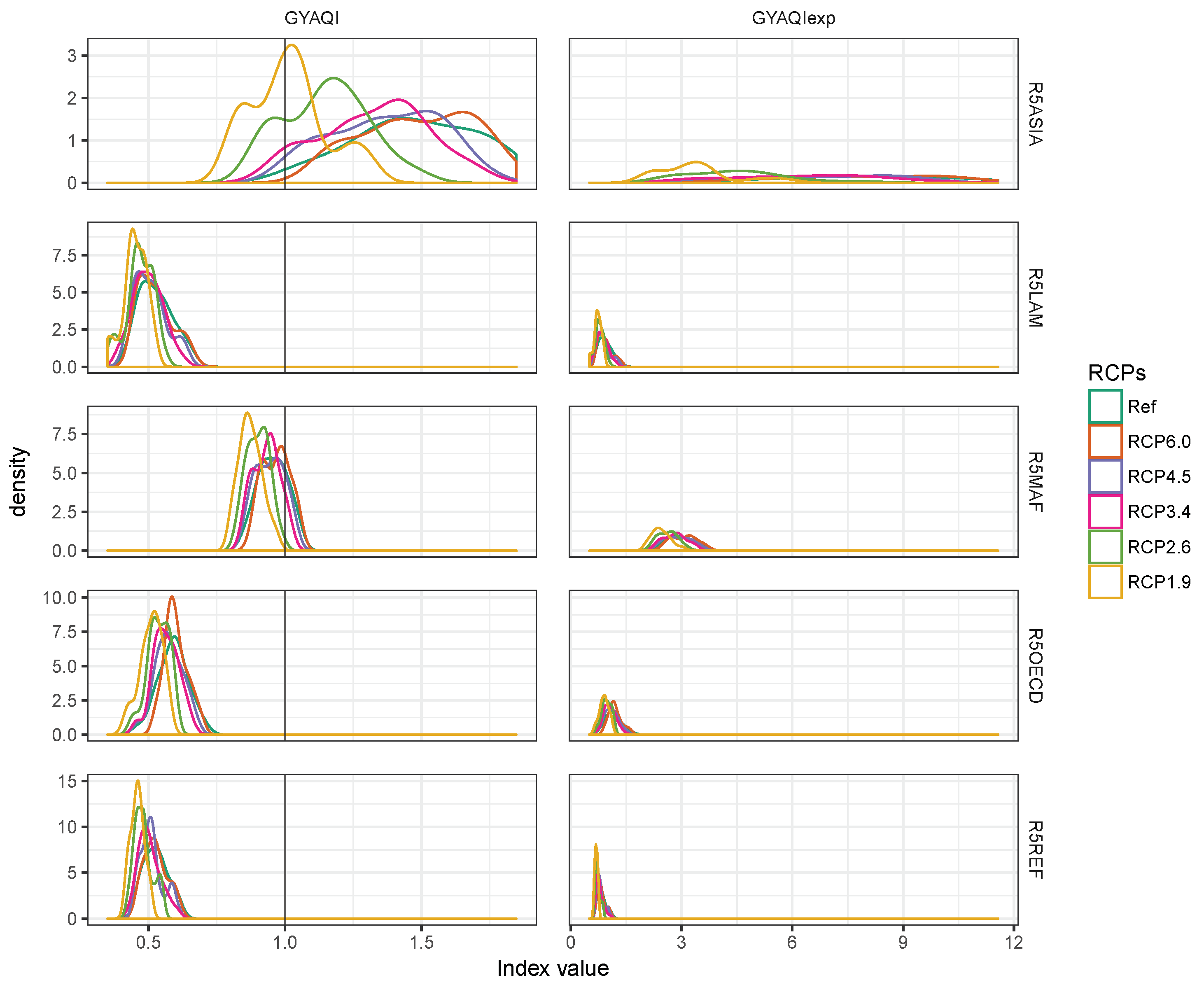
We have shown that both SSPs and climate policies play a role in air quality improvement. However, climate policies are generally more effective after 2030 in reducing air pollution, especially from ozone. The underlying assumptions behind the SSPs, on the other hand, seem to be more effective for PM${}_{2.5}$ reductions, and have a greater impact on the magnitude of the results, while climate policies influence the speed of the reductions. This is visible in Figure A5 and Figure A6, where the “greener” socioeconomic assumptions (SSP1) show a narrower range than a 2 ${}^{\circ }$C policy (RCP2.6) across SSPs. Interestingly, however, the climate target set by the Paris agreement (1.5 ${}^{\circ }$C, i.e., RCP1.9) reverses this trend narrowing the indices probability distribution more than SSP1. All models agree that a 1.5 ${}^{\circ }$C policy would prevent all regions of the world from exceeding the annual population-weighted average limit of the multi-pollutant index (GYAQI) and of the sub-indices (${\psi }_p$) of all the pollutants, except PM${}_{2.5}$.

Figure A5 shows that, when comparing the socioeconomic assumptions, SSP1 is the scenario where better air quality is achieved. In fact, in SSP1, the distribution always dominates the other SSPs. This is especially important when comparing with SSP5, which assumes the same emission controls as SSP1, but varies regarding energy use and other drivers, meaning that even when employing the best air pollution controls, the exploitation of fossil fuels and the use of energy intensive lifestyles is not compatible with the lowest achievements in terms of air pollution controls. The exception is the OECD region, where climate and air quality policies are already at a more advanced stage and climate policies have a lower impact. SSP3 is undoubtedly, as all models agree, the most problematic of the scenarios in terms of air quality, not only because it is incompatible with the most stringent climate policies, but also due to its air pollution control assumptions. On the contrary, the socioeconomic conditions of SSP5 are a threat to climate goals but are relatively advantageous from an air quality point of view. It is the overall evaluation of both goals that will determine the optimal policy. Overall, we find thus that the most sustainable socioeconomic development policy (SSP1) is also the one that yields better air quality and that increases the changes of climate policy success.

4.2. Regional Focus

The Asian region is the most challenging in terms of air quality compliance. OECD shows the highest improvements and Latin America poses the lowest pollution challenges. Different regions will experience different challenges: ozone is a pollutant of concern especially in OECD and Middle East and Africa, whereas PM${}_{2.5}$ will require particular attention worldwide, and especially in Asia where the population will be exposed to extreme concentrations in all regions. Additionally, we have explored the AQIs in some of the major economies, such as China, India, USA, and the European Union. China pollution peaks earlier than India, and shows in general a descending trend independently of the socioeconomic assumptions. However, when a climate policy is enforced in India, air pollution shows a steep descending pathway due to its lower CO${}_2$ marginal abatement costs. As carbon emissions are generally related to air pollution emissions, the fact that climate policy acts were the carbon abatement costs are lower will bring faster improvements to air quality helping to avoid more premature deaths. In this sense, climate policies, such as international agreements on limiting the average temperature increase will substantially reduce air pollution, especially for the regions where improvements are more important and affordable, such as India and China. In what concerns the developed economies, we found that the European Union experiences lower levels of the AQIs.

4.3. Choosing the Adequate AQI

We have explored several types of AQIs that can be used in global mid to long term integrated policy evaluation and to measure air quality co-benefit of global policies. We have discussed their adequacy and the pros and cons of each of the AQIs. They are presented in

Table 4. Strengths and limitations of the AQIs.

AQIs	Strengths	Limitations
GYAQI	Multi-pollutant; easy formulation	Very sensitive to averages; requires analysis of the pollutant sub-indices; does not provide information on fractions of exposed population
GYAQIv	Multi-pollutant; focus on the most problematic pollutants	Does not provide information on fractions of exposed population
GYAQIvm	Multi-pollutant; not pollutant sensitive; highlights single pollutant problems	Does not provide information on fractions of exposed population
GYAQIexp	Multi-pollutant; accounts for population exposure	Does not provide a direct measure of impact on human heath
AQLI	Provides a direct measure of impact on human heath	Only takes into account PM${}_{2.5}$

which summarizes our discussion of the different AQIs.

The multi-pollutant averaged air quality index “hides” possible concerns when other sub-indices are low enough to bring the average index down. The AQI variants (GYAIQv and GYAIQvm) isolate the effect of the most problematic pollutants, further highlighting the air pollution issue in Asia and bringing to light other potential problems in the other regions. Additionally, we present AQIs, such as the GYAQIexp and the AQLI, that consider population exposure to high and very high levels of pollution even when the greater annual regional average performs well. We conclude that the exposure AQIs are more adequate in the context of global policy because they provide more information and still allow for a single value score when comparing several integrated policies.

The construction of a composite index entails a loss of information. Nevertheless, it is very useful for many other reasons, such as general public information and awareness, civil society organizations, and policy making. As noted by Khordagui and Al-Ajmi [41], indices can be used not only to inform the public but also to assist policy making either by evaluating air pollution measures or by supporting the policy optimization and ultimately to control legislative compliance.

The exposure AQIs proposed in this paper are useful for policy-makers when negotiating future climate commitments having in mind the regional air pollution pathways. They help to place future air quality in a range of plausible futures that might unfold. Additionally, as in this work, the new AQIs can be used to represent the health dimension when considering a multi-criteria welfare analysis of sustainable policies taking into account not only climate and pollution objectives but also socioeconomic goals. In this case, a single value is needed to aggregate comprehensive and valuable information on pollution impacts across a range of complex integrated policy scenarios. Finally, the SSP–RCP scenario analysis informs on the possible co-benefits of climate and socioeconomic policy providing top-down insights into annual regional air pollution levels which in turn could be used by higher resolution models to better study the local impacts of these policies.

4.4. Future Research

Our results isolate the effect of emission pathways on population-weighted averages to be able to detect how the SSP and RCP air pollution emission pathways impact the AQIs. This is undertaken by keeping the population patterns frozen for all scenarios when calculating the concentrations and not allowing the results to vary with population growth. A topic of future research could be the evaluation of how population growth and changes in population density spatial patterns affect exposure and the AQIs.

Additionally, as air pollution is just one of the aspects that qualify the impact of a policy, a major step forward would be to develop indicators for other aspects, such as biodiversity, water demand, land-use, forest management and equity and equality to be able to have an more complete integrated evaluation of the global policies. Moreover, although the AQLI already provides a measure of health impacts, in this study, we did not look into the cost of these policies or into how these scenarios would translate in terms of mortality numbers, which could be a line of further research.

References

1. United Nations (UN). Transforming Our World: The 2030 Agenda for Sustainable Development; Technical Report; United Nations: New York, NY, USA, 2015. [Google Scholar]
2. Riahi, K.; van Vuuren, D.P.; Kriegler, E.; Edmonds, J.; O’Neill, B.C.; Fujimori, S.; Bauer, N.; Calvin, K.; Dellink, R.; Fricko, O.; et al. The Shared Socioeconomic Pathways and their energy, land use, and greenhouse gas emissions implications: An overview. Glob. Environ. Chang. 2017, 42, 153–168. [Google Scholar] [CrossRef] [Green Version]
3. Srinath Reddy, K. Global Burden of Disease Study 2015 provides GPS for global health 2030. Lancet 2016, 388, 1448–1449. [Google Scholar] [CrossRef]
4. World Health Organizatio (WHO). WHO Expert Meeting: Methods and Tools for Assessing the Health Risks of Air Pollution at Local, National and International Level; Technical Report 109.2015; WHO: Bonn, Germany, 2014. [Google Scholar]
5. World Health Organizatio (WHO). Review of Evidence on Health Aspects of Air Pollution—REVIHAAP Project; Technical Report 109.2015; WHO: Bonn, Germany, 2014. [Google Scholar]
6. West, J.J.; Smith, S.J.; Silva, R.A.; Naik, V.; Zhang, Y.; Adelman, Z.; Lamarque, J.F. Co-benefits of Global Greenhouse Gas Mitigation for Future Air Quality and Human Health. Nat. Clim. Chang. 2013, 3, 885–889. [Google Scholar] [CrossRef] [PubMed]
7. Rao, S.; Klimont, Z.; Leitao, J.; Riahi, K.; van Dingenen, R.; Reis, L.A.; Calvin, K.; Dentener, F.; Drouet, L.; Fujimori, S.; et al. A multi-model assessment of the co-benefits of climate mitigation for global air quality. Environ. Res. Lett. 2016, 11, 124013. [Google Scholar] [CrossRef] [Green Version]
8. Rao, S.; Klimont, Z.; Smith, S.J.; Dingenen, R.V.; Dentener, F.; Bouwman, L.; Riahi, K.; Amann, M.; Bodirsky, B.L.; van Vuuren, D.P.; et al. Future air pollution in the Shared Socio-economic Pathways. Glob. Environ. Chang. 2017, 42, 346–358. [Google Scholar] [CrossRef] [Green Version]
9. Van Vuuren, D.P.; Kriegler, E.; O’Neill, B.C.; Ebi, K.L.; Riahi, K.; Carter, T.R.; Edmonds, J.; Hallegatte, S.; Kram, T.; Mathur, R.; et al. A new scenario framework for Climate Change Research: Scenario matrix architecture. Clim. Chang. 2014, 122, 373–386. [Google Scholar] [CrossRef]
10. Jiang, L.; O’Neill, B.C. Global urbanization projections for the Shared Socioeconomic Pathways. Glob. Environ. Chang. 2017, 42, 193–199. [Google Scholar] [CrossRef] [Green Version]
11. Van Vuuren, D.P.; Edmonds, J.; Kainuma, M.; Riahi, K.; Thomson, A.; Hibbard, K.; Hurtt, G.C.; Kram, T.; Krey, V.; Lamarque, J.F.; et al. The representative concentration pathways: An overview. Clim. Chang. 2011, 109, 5. [Google Scholar] [CrossRef]
12. Shooter, D.; Brimblecombe, P. Air quality Indexing. Int. J. Environ. Pollut. 2008, 36, 305–323. [Google Scholar] [CrossRef]
13. Plaia, A.; Ruggieri, M. Air quality indices: A review. Rev. Environ. Sci. Bio/Technol. 2011, 10, 165–179. [Google Scholar] [CrossRef]
14. Gorai, A.K.; Kanchan; Upadhyay, A.; Tuluri, F.; Goyal, P.; Tchounwou, P.B. An innovative approach for determination of air quality health index. Sci. Total Environ. 2015, 533, 495–505. [Google Scholar] [CrossRef] [PubMed] [Green Version]
15. Robichaud, A. Surface data assimilation of chemical compounds over North America and its impact on air quality and Air Quality Health Index (AQHI) forecasts. Air Qual. Atmos. Health 2017, 10, 955–970. [Google Scholar] [CrossRef] [PubMed] [Green Version]
16. Elshout, S.V.D.; Bartelds, H.; Heich, H.; Leger, K. CAQI Air Quality Index; Technical Report; DCMR and EUROPEAN UNION European Regional Development Fund Regional Initiative Project: Brussels, Belgium, 2012. [Google Scholar]
17. Energy Policy Institute. The Air Quality-Life Index (AQLI); University of Chicago: Chicago, IL, USA, 2017. [Google Scholar]
18. Anenberg, S.; Horowitz, L.; Tong, D.; West, J. An estimate of the global burden of anthropogenic ozone and fine particulate matter on premature human mortality using atmospheric modeling. Environ. Health Perspect. 2010, 118, 1189–1195. [Google Scholar] [CrossRef] [PubMed]
19. IIASA Energy Program. SSP Database (Shared Socioeconomic Pathways)—Version 11. Available online: https://tntcat.iiasa.ac.at/SspDb (accessed on 11 October 2018).
20. Fujimori, S.; Hasegawa, T.; Masui, T.; Takahashi, K.; Herran, D.S.; Dai, H.; Hijioka, Y.; Kainuma, M. SSP3: AIM implementation of Shared Socioeconomic Pathways. Glob. Environ. Chang. 2017, 42, 268–283. [Google Scholar] [CrossRef]
21. Calvin, K.; Bond-Lamberty, B.; Clarke, L.; Edmonds, J.; Eom, J.; Hartin, C.; Kim, S.; Kyle, P.; Link, R.; Moss, R.; et al. The SSP4: A world of deepening inequality. Glob. Environ. Chang. 2017, 42, 284–296. [Google Scholar] [CrossRef]
22. Van Vuuren, D.P.; Stehfest, E.; Gernaat, D.E.; Doelman, J.C.; van den Berg, M.; Harmsen, M.; de Boer, H.S.; Bouwman, L.F.; Daioglou, V.; Edelenbosch, O.Y.; et al. Energy, land-use and greenhouse gas emissions trajectories under a green growth paradigm. Glob. Environ. Chang. 2017, 42, 237–250. [Google Scholar] [CrossRef]
23. Fricko, O.; Havlik, P.; Rogelj, J.; Klimont, Z.; Gusti, M.; Johnson, N.; Kolp, P.; Strubegger, M.; Valin, H.; Amann, M.; et al. The marker quantification of the Shared Socioeconomic Pathway 2: A middle-of-the-road scenario for the 21st century. Glob. Environ. Chang. 2017, 42, 251–267. [Google Scholar] [CrossRef] [Green Version]
24. Kriegler, E.; Bauer, N.; Popp, A.; Humpenöder, F.; Leimbach, M.; Strefler, J.; Baumstark, L.; Bodirsky, B.L.; Hilaire, J.; Klein, D.; et al. Fossil-fueled development (SSP5): An energy and resource intensive scenario for the 21st century. Glob. Environ. Chang. 2017, 42, 297–315. [Google Scholar] [CrossRef]
25. Emmerling, J.; Drouet, L.; Reis, L.A.; Bevione, M.; Berger, L.; Bosetti, V.; Carrara, S.; Cian, E.D.; D’Aertrycke, G.D.M.; Longden, T.; et al. The WITCH 2016 Model—Documentation and Implementation of the Shared Socioeconomic Pathways; Working Paper 2016.42; Fondazione Eni Enrico Mattei: Milan, Italy, 2016. [Google Scholar]
26. Intergovernmental Panel on Climate Change (IPCC). Climate Change 2014: Synthesis Report; Contribution of Working Groups I, II and III to the Fifth Assessment Report of the Intergovernmental Panel on Climate Change; Technical Report; IPCC: Geneva, Switzerland, 2014; 151p. [Google Scholar]
27. Krol, M.; Houweling, S.; Bregman, B.; van den Broek, M.; Segers, A.; van Velthoven, P.; Peters, W.; Dentener, F.; Bergamaschi, P. The two-way nested global chemistry-transport zoom model TM5: algorithm and applications. Atmos. Chem. Phys. 2005, 5, 417–432. [Google Scholar] [CrossRef]
28. Leitao, J.; Van Dingenen, R.; Rao, S. Report on Spatial Emissions Downscaling and Concentrations for Health Impacts Assessment; Technical Report 109.2015; IIASA: Milan, Italy, 2013. [Google Scholar]
29. Van Dingenen, R.; Dentener, F.; Crippa, M.; Leitao, J.; Marmer, E.; Rao, S.; Solazzo, E.; Valentini, L. TM5-FASST: A global atmospheric source-receptor model for rapid impact analysis of emission changes on air quality and short-lived climate pollutants. Atmos. Chemi. Phys. Discuss. 2018, 2018, 1–55. [Google Scholar] [CrossRef]
30. GEA. Global Energy Assessment: Toward a Sustainable Future; Cambridge University Press: Cambridge, UK, 2017. [Google Scholar]
31. Elshout, S.V.D.; Leger, K.; Heich, H. {CAQI} Common Air Quality Index ? Update with PM2.5 and sensitivity analysis. Sci. Total Environ. 2014, 488–489, 461–468. [Google Scholar] [CrossRef] [PubMed]
32. Olivares, A.; van Drooge, B.L.; Ballesta, P.P.; Grimalt, J.O.; Piña, B. Assessment of dioxin-like activity in ambient air particulate matter using recombinant yeast assays. Atmos. Environ. 2011, 45, 271–274. [Google Scholar] [CrossRef]
33. Li, H.; Qian, X.; Wang, Q. Heavy Metals in Atmospheric Particulate Matter: A Comprehensive Understanding Is Needed for Monitoring and Risk Mitigation. Environ. Sci. Technol. 2013, 47, 13210–13211. [Google Scholar] [CrossRef] [PubMed]
34. Gulia, S.; Nagendra, S.S.; Khare, M.; Khanna, I. Urban air quality management-A review. Atmos. Pollut. Res. 2015, 6, 286–304. [Google Scholar] [CrossRef]
35. Organisation for Economic Co-operation and Development (OECD). The Economic Consequences of Outdoor Air Pollution; Organisation for Economic Co-Operation and Development Publishing: Paris, France, 2016. [Google Scholar]
36. Forouzanfar, M.H.; Afshin, A.; Alexander, L.T.; Anderson, H.R.; Bhutta, Z.A.; Biryukov, S.; Brauer, M.; Burnett, R.; Cercy, K.; Charlson, F.J.; et al. Global, regional, and national comparative risk assessment of 79 behavioural, environmental and occupational, and metabolic risks or clusters of risks, 1990–2015: A systematic analysis for the Global Burden of Disease Study 2015. Lancet 2016, 388, 1659–1724. [Google Scholar] [CrossRef]
37. Dingenen, R.V.; Dentener, F.J.; Raes, F.; Krol, M.C.; Emberson, L.; Cofala, J. The global impact of ozone on agricultural crop yields under current and future air quality legislation. Atmos. Environ. 2009, 43, 604–618. [Google Scholar] [CrossRef]
38. Janhall, S. Review on urban vegetation and particle air pollution—Deposition and dispersion. Atmos. Environ. 2015, 105, 130–137. [Google Scholar] [CrossRef]
39. Babcock, J.R.; Lyndon, R. A combined pollution index for measurement of total air pollution. J. Air Pollut. Control Assoc. 1970, 20, 653–659. [Google Scholar] [CrossRef] [PubMed]
40. Kanchan, K.; Gorai, A.; Goyal, P. A Review on Air Quality Indexing System. Asian J. Atmos. Environ. 2015, 9, 101–113. [Google Scholar] [CrossRef] [Green Version]
41. Khordagui, H.K.; Al-Ajmi, D.N. Application of indices for air quality management in Kuwait. Environ. Manag. 1996, 20, 151–158. [Google Scholar] [CrossRef]
42. Kriegler, E.; Edmonds, J.; Hallegatte, S.; Ebi, K.L.; Kram, T.; Riahi, K.; Winkler, H.; van Vuuren, D.P. A new scenario framework for climate change research: The concept of shared climate policy assumptions. Clim. Chang. 2014, 122, 401–414. [Google Scholar] [CrossRef]
Figure 1. The GYAQI of all regions, across the SSP and RCP scenario matrix. The shaded area represents the IA model range. Total Radiative Forcing (TRF) in 2100 in the reference (“Ref”) scenario is shown for comparison with the climate policies. The colors of the SSP labels represent the level of implementation of air pollution control policies in the SSP narratives: green represents the strongest deployment of air pollution control measures and red represents the poorest.
Sustainability 10 03645 g001
Figure 2. The GYAQIv, and the subindices ψ p for the region of Asia, across the SSP and RCP scenario matrix. The shaded area represents the IA model range. Total Radiative Forcing (TRF) in 2100 in the reference scenario is shown for comparison with the climate policies. The colors on the SSP labels represent the level of implementation of air pollution control policies in the SSP narratives: green represents the strongest deployment of air pollution control measures and red represents the poorest.
Sustainability 10 03645 g002
Figure 3. Comparison of the GYAQI, GYAQIv, GYAQIvm, GYAQIexp and AQLI for the region of Asia, across the SSP and RCP scenario matrix. The shaded area represents the IA model range. Total Radiative Forcing (TRF) in 2100 in the reference scenario is presented for comparison with the climate policies. The colors on the SSP labels represent the level of implementation of air pollution control policies in the SSP narratives: green represents the strongest deployment of air pollution control measures and red represents the poorest.
Sustainability 10 03645 g003
Figure 4. Comparison of the GYAQI, GYAQIv, GYAQIvm, GYAQIexp and AQLI for the countries of China and India, across the SSP and RCP scenario matrix. The shaded area represents the Shared climate Policy Assumption scenario range. Total Radiative Forcing (TRF) in 2100 in the reference scenario is presented for comparison with the climate policies. The colors on the SSP labels represent the level of implementation of air pollution control policies in the SSP narratives: green represents the strongest deployment of air pollution control measures and red represents the poorest.
Sustainability 10 03645 g004
Figure 5. Representation of the workflow for the calculation of the AQI.
Sustainability 10 03645 g005