Reduced Inequalities as Factor of Sustainable Development: The Analysis Under Econometric Models

Abstract

The paper proposes a different approach for the analysis of the sustainable development in the context of 2030 Agenda. The authors defined and used a cumulative model. For the beginning, the authors compare the dependent variable with the regressors of the four reporting entities: EU28, Romania, Turkey and Switzerland. These entities cover EU, the country of the authors, a candidate country and non-EU country, as well. The analysis is focused on the Goal 10 from the 2030 Agenda Sustainable Development, covers 2000–2017 and is based on the latest official data from Eurostat. The model used by the authors generated high statistical representativeness. The statistical tests demonstrate the model’s homogeneity. A distinct part of the paper is focused on the risk analysis. The authors basically propose a distinct approach which is usefully for the central and regional decision makers. The statistical period took into consideration is good enough to support pertinent conclusions. The analysis leads to the conclusion that Romania can decrease the disparities regarding the sustainable development. On the other hand, the Romania’s progress in achieving sustainable development’s targets is lowest than the EU average. The model proposed in the paper supports the decision makers in achieving a more performant management regarding sustainable development goals. The paper represents a theoretical approach with great applicability to economic development.

1. Introduction

The implementation of a new sustainable development agenda was finally accepted on September 2015 [1]. The United Nations established 17 goals for the next 15 years, in order to ensure poverty’s end, planet’s protection and prosperity for all.

The European Union, as regional organisation, adopted the sustainable development agenda and pointed out its approach on this [2].

According to the above two documents, the 2030 Agenda Sustainable Development goals are the following:

• end poverty in all its forms everywhere;
• end hunger, achieve food security and improved nutrition and promote sustainable agriculture;
• ensure healthy lives and promote well-being for all at all ages;
• ensure inclusive and equitable quality education and promote lifelong learning opportunities for all;
• achieve gender equality and empower all women and girls;
• ensure availability and sustainable management of water and sanitation for all;
• ensure access to affordable, reliable, sustainable and modern energy for all;
• promote sustained, inclusive and sustainable economic growth, full and productive employment and decent work for all;
• build resilient infrastructure, promote inclusive and sustainable industrialization and foster innovation;
• reduce inequality within and among countries;
• make cities and human settlements inclusive, safe, resilient and sustainable;
• ensure sustainable consumption and production patterns;
• take urgent action to combat climate change and its impacts;
• conserve and sustainably use the oceans, seas and marine resources for sustainable development;
• protect, restore and promote sustainable use of terrestrial ecosystems, sustainably manage forests, combat desertification, and halt and reverse land degradation and halt biodiversity loss;
• promote peaceful and inclusive societies for sustainable development, provide access to justice for all and build effective, accountable and inclusive institutions at all levels;
• strengthen the means of implementation and revitalize the Global Partnership for Sustainable Development.

The present paper points out the idea of using a different approach in analysing the Agenda’s goals starting to the 10th goal (reduce inequality within and among countries). The same analysis can be extended to the other 16 goals, as well.

This approach is different from that of Ming-Chuan Y., Qiang M., Sang-Bing T. and Yi D., who analysed the 8th goal connected to innovation [3]. Other specialists pointed out the impact of the unsustainable development on socio-economic and environment trends [4].

A distinct approach puts into analysis the urban sustainability under the new challenges related to urban population increasing and climate change [5]. Some researchers are focused on sustainability for different industries. One of them proposes a sustainability index for the automotive industry [6].

In the same way, other research analyses the sustainability of the water consumption and pollution across the Latin America and Caribbean [7]. The importance of the sustainable development led to the need of defining and building business models for sustainability [8,9,10,11,12].

An interesting review of the literature on sustainability transitions covers 386 journal articles during 1995–2014 and concludes that the role of actors and agency in this literature is very complex [13]. The need of a sustainable urban development was connected to the cities’ key role for general development across the world [14].

A distinct research realises the connection between sustainability and circular economy. The paper succeeds in finding eight different relationship types able to point out the similarities and differences between sustainability and circular economy [15].

The best facing to the sustainability’s challenges is the collaboration between government, business environment and stakeholders. More, the government would be incorporated again into the models of effective corporate governance [16].

An interesting approach takes into consideration the mechanisms which perceived job insecurity influences both mental and physical health and on the effect of unemployment on depression [17].

The sustainability depends on investment. This is why the national budget has an important impact in the sustainable development. The connection between budget and sustainability in candidate countries becomes very important [18].

On the other hand, the sustainability can be analysed in connection with Europe 2020 Strategy, which is focused on economic performance and competitiveness [19].

The same competitiveness is pointed out at industrial level in a very interesting paper [20].

The above literature leads to the conclusion of defining and implementing of new performant models for sustainable development. The present paper proposes such models.

2. Materials, Model, and Methods

The model proposed in this paper is applied to the following economic entities: EU28, Romania, Turkey, and Switzerland. We choose Romania as first analysed entity because is one European state with high economic growth and big gap on sustainable development. Moreover, the latest two economic entities were chosen as candidate EU country and as non-EU country in the same Europe, because we wanted to cover whole diversity of the economic sustainability across Europe.

The model takes into consideration the average trend for 43 economic entities, including the Member States and other non-EU economies (The all 43 economic entities cover: EU-28, EU-27, EU-19, EU-18, Belgium, Bulgaria, Czech Republic, Denmark, Germany, Estonia, Ireland, Greece, Spain, France, Croatia, Italy, Cyprus, Latvia, Lithuania, Luxembourg, Hungary, Malta, Netherlands, Austria, Poland, Portugal, Romania, Slovenia, Slovakia, Finland, Sweden, United Kingdom, Iceland, Norway, Switzerland, Montenegro, Former Yugoslav Republic of Macedonia, Albania, Serbia, Turkey, Bosnia and Herzegovina, United States and Japan). The analysis covers 2000–2017 and is based on the latest official data from Eurostat. The same analysis is focused on the Goal 10 from the 2030 Agenda Sustainable Development, which points out specific sustainable development indicators. The model is representing our original approach.

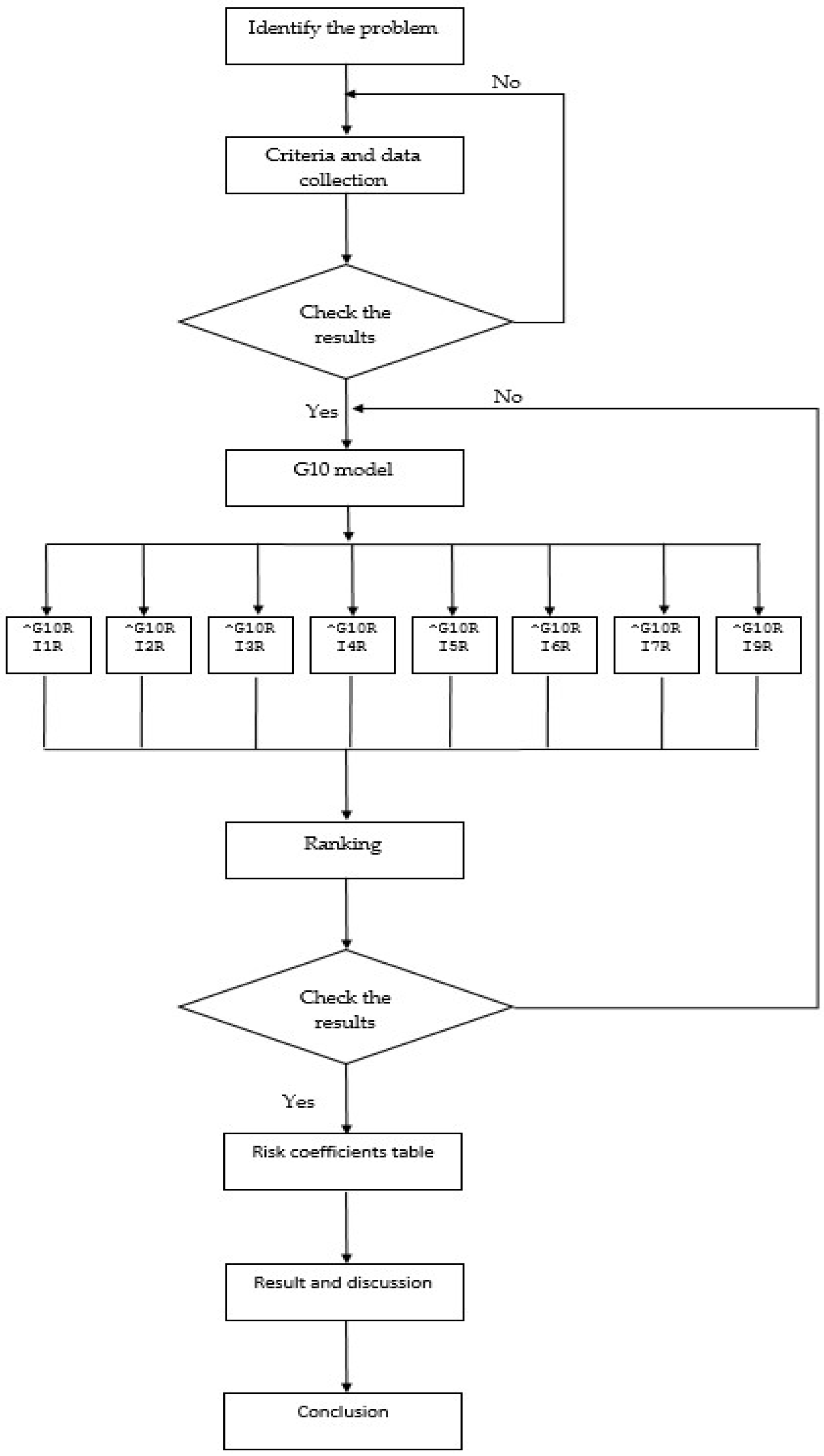
Figure 1 presents the research analysis scheme which covers three steps. The first step points out the identification procedure in data collecting, the building of the data basis and the indicators used in analysis, including literature review for identifying similarly models or experts’ opinion in the area. This step is the same as conceptualisation and its finalisation and validation allow the access to the second step: model defining and statistical testing of the 8 points from 10th goal of the Strategy.

The resulted data are tested under statistical procedures and the model validation allows the pass to the final step: the risk table’s building, research’s conclusions and dissemination.

The model’s hypotheses in this analysis are the following:

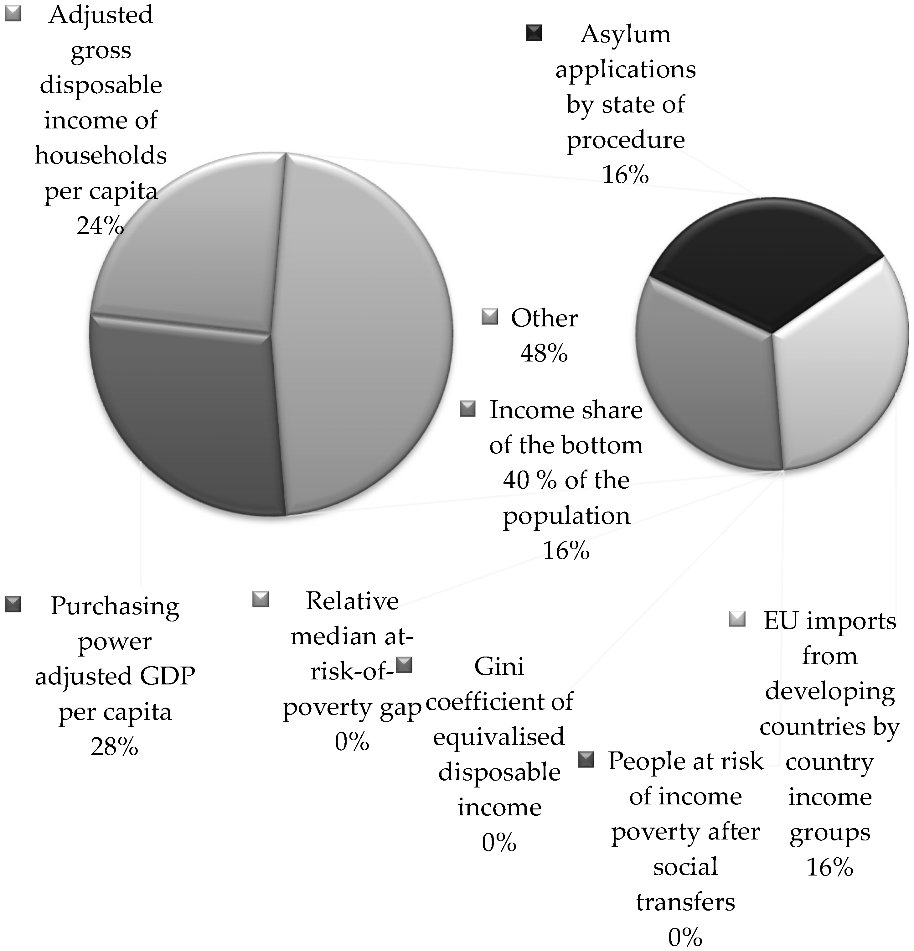
• the proposed model uses the indicators: Purchasing power adjusted GDP per capita; Adjusted gross disposable income of households per capita; Relative median at-risk-of-poverty gap; Gini coefficient of equivalised disposable income; Income share of the bottom 40% of the population; Asylum applications by state of procedure; People at risk of income poverty after social transfers; EU imports from developing countries by country income groups. The 8-th indicators took into analysis are those from the Goal 10.8 from 2030 Agenda;
• the analysis doesn’t take into consideration the Goal 10.8 from 2030 Agenda, because of the lack of data for this indicator;
• the analysed indicators present an oscillating trend, which is optimally represented by the trend line estimated for the EU28;
• Romanian economy’s statue within the analysed economic entities is quantified using the dynamic averages’ evolution or by reference to Turkey, Switzerland, EU28 and general average’s trends;
• the gaps between Romanian economy and the other analysed economic entities quantify the challenges regarding the sustainable development which Romania records in relation to EU28 policy according to 2030 Agenda;
• the forecasting sustainability model regarding Romania’s performances improving in relation to Goal 10 from 2030 Agenda can be developed by mathematical quantification of the gaps;
• The analysis covers n = 17 years (2000–2017), in order to have enough time period. This period defines the time between Romania’s adhering starting negotiations (15 February 2000, Romania’s adhering to the EU (1 January 2007) and the economic post-adhering progresses.

In order to realise the sustainability analysis, the paper used the Eurostat’s data for all 43 economic entities. Moreover, the analysis quantified 43 trend statistical averages and realised tend analyses using mobile average computing to Romania, EU28, Turkey and Switzerland [17].

The statistical data on 2000–2017 have been disseminated statistically, using the impact weights, in order to calculate Romania’s sustainable development gaps in relation to the four reporting entities.

As a result, the general evolution table for the eight indicators from the 1st hypothesis was built. The data were translated by the dedicated software Gretl to models of sustainability analysis for each indicator. It is used as a platform for econometric analysis. The latest version of the software is Gretl-2018b. The models are cumulative and compare the dependent variable with the regressors of the four reporting entities. The general model can be defined as:

$$\mathrm{V}=\alpha V_1+\beta V_2+\gamma V_3+\delta V_4+\epsilon ,$$

(1)

where V—dependent variable for Romania relative to each indicator presented under 1s hypothesis; V₁–V₄—regressors obtained by reporting Romania’s trends to each of the 4 reporting entities; $\alpha ,\beta ,\gamma ,\delta$—regression coefficients; $\epsilon$—residual variable.

The data has been modelled in order to validate the model by calculating statistical representativeness, homogeneity and data consistency and obtaining information on the relevance of the model for the analysed phenomenon.

3. Results

The applying of the general model to the Goal 10 indicators in 2030 Agenda leads to the following conclusions.

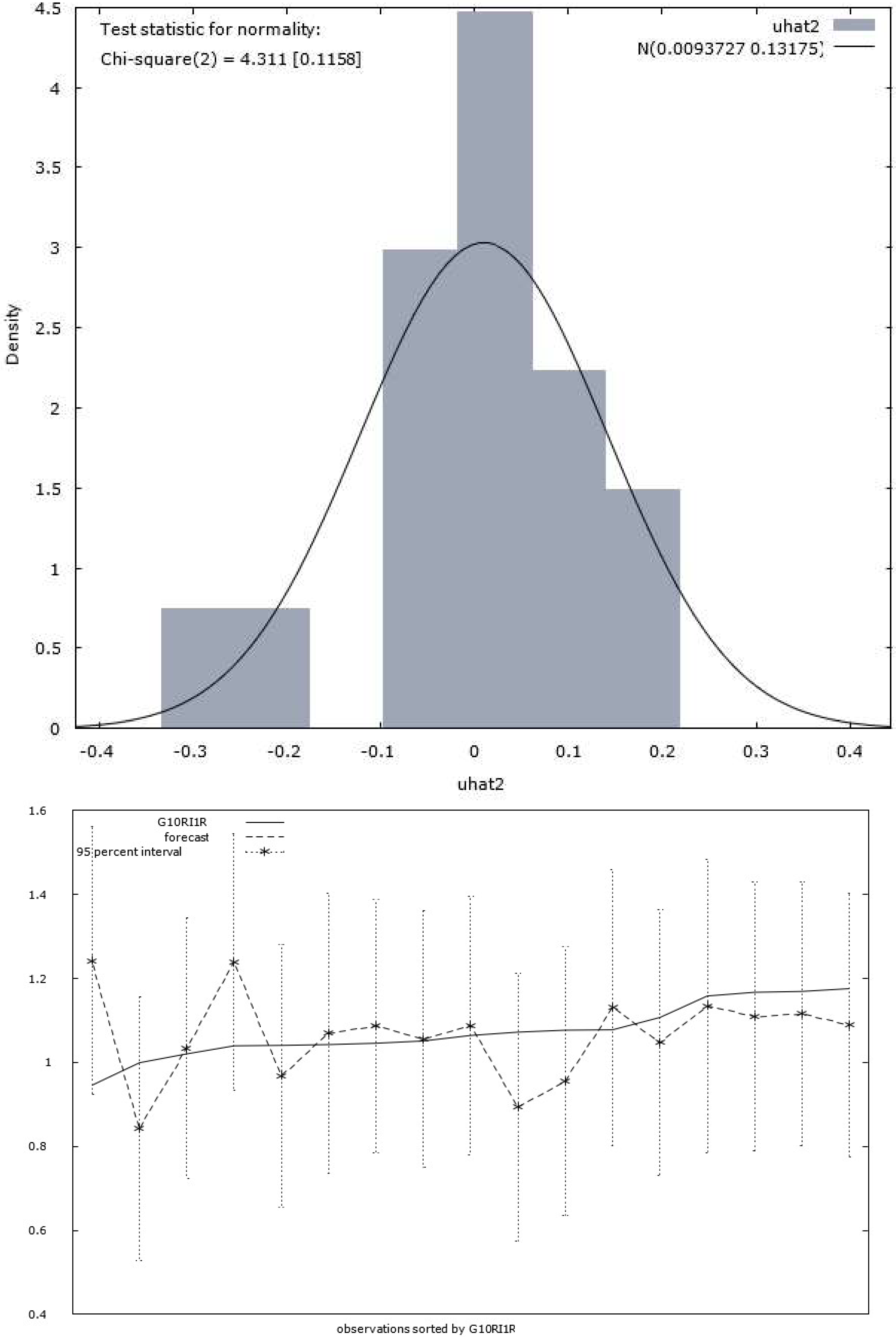
The model generated a statistical representativeness of 0.988 for “Purchasing power adjusted GDP per capita (G10RI1)” (

Table 1. Ordinary least squares (OLS), using observations 1–17; Dependent variable: G10RI1R.

	Coefficient		Std. Error		t-Ratio	p-Value
G10RI1R_AVG	18.0785		11.6972		1.5455	0.14621
G10RI1R_S	6.22996		6.08452		1.0239	0.32456
G10RI1R_T	0.607992		0.597181		1.0181	0.32720
G10RI1R_EU28	−21.8376		12.0616		−1.8105	0.09338		*
Mean Dependent var		1.073940		S.D. Dependent var			0.063721
Sum squared resid		0.227152		S.E. of regression			0.132186
R-squared		0.988453		Adjusted R-squared			0.985788
F(4, 13)		278.2068		p-value (F)			1.89 × 10−12
Log-likelihood		12.55850		Akaike criterion			−17.11700
Schwarz criterion		−13.78415		Hannan-Quinn			−16.78571

*: The regression coefficients are proving that the probability density function is disturbed at 0.14, and the figures have medium statistical significance. Test for normality of residual; Null hypothesis: error is normally distributed; Test statistic: Chi-square (2) = 4.31103; with p-value = 0.115843.

). Moreover, the value for test F is close to 0 and the error is normally distributed for the Chi-square statistical test. The equation for the smallest squares regression model is:

^G10RI1R = + 18.1*G10RI1R_AVG + 6.23*G10RI1R_S + 0.608*G10RI1R_T − 21.8*G10RI1R_EU28						(2)
	(11.7)	(6.08)		(0.597)	(12.1)
n = 17, R-squared = 0.988
(standard errors in parentheses)

The statistical tests demonstrate the model’s homogeneity:

The histogram distribution and prediction diagrams on the confidence interval of 95% estimate a homogenic distribution for the dependent variable in relation to the regression variable (see Figure 2).

Forecast evaluation statistics:

• Mean Error: 0.0093727
• Mean Squared Error: 0.013362
• Root Mean Squared Error: 0.11559
• Mean Absolute Error: 0.086206
• Mean Percentage Error: 0.57368
• Mean Absolute Percentage Error: 8.2609
• Theil’s U 1.5248
• Bias proportion, UM 0.0065744
• Regression proportion, UR 0.70939
• Disturbance proportion, UD 0.28404

The model quantifies the indicator Purchasing power adjusted GDP per capita (G10RI1) and points out that Romania is broadly in line with its sustainability objectives promoted by 2030 Agenda for this indicator.

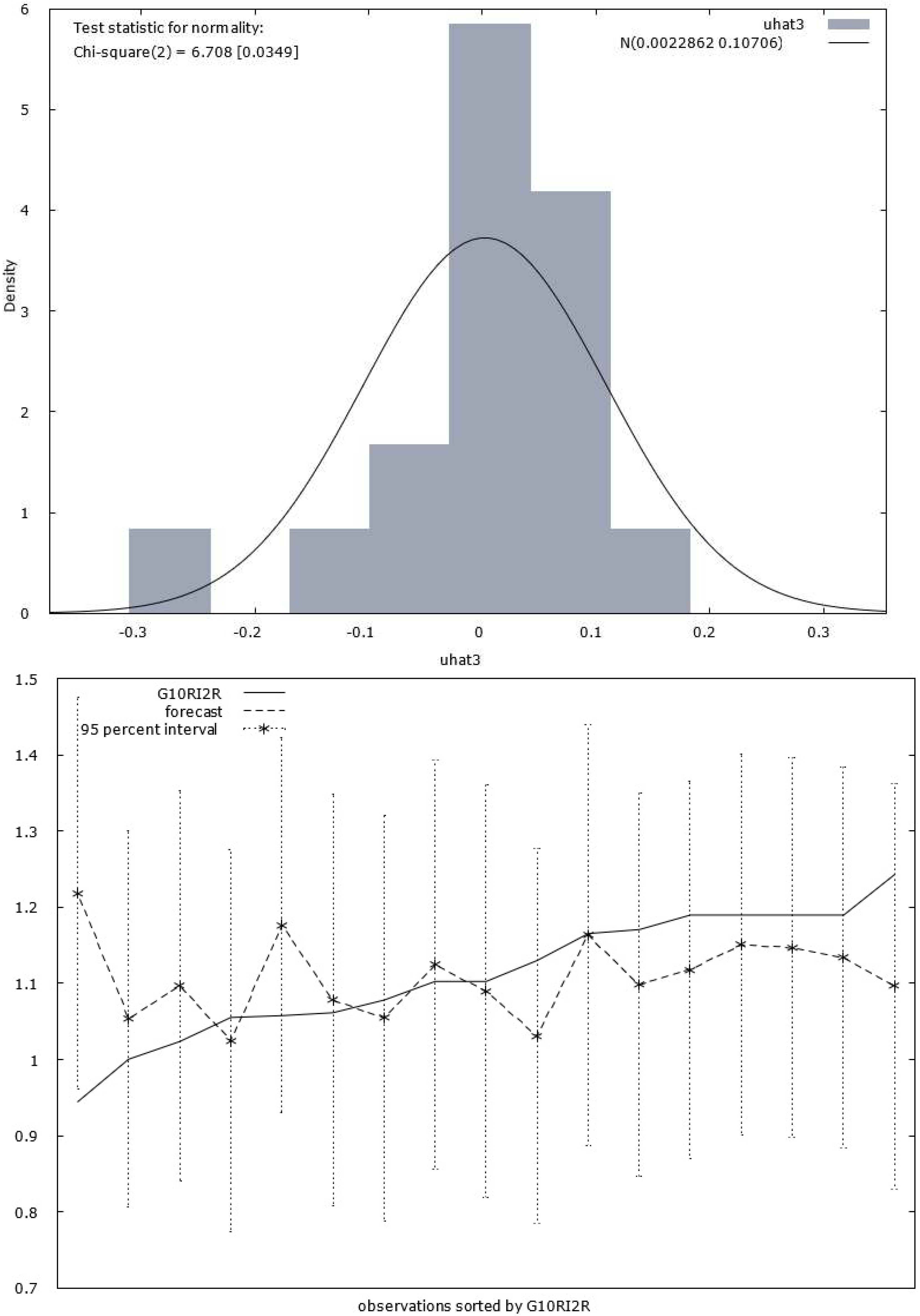
The second indicator, “Adjusted gross disposable income of households per capita (G10RI2)” (

Table 2. OLS, using observations 1–17; Dependent variable: G10RI2R.

	Coefficient		Std. Error		t-Ratio	p-Value
G10RI2R_AVG	13.4652		8.67884		1.5515	0.14478
G10RI2R_S	−4.43451		5.86473		−0.7561	0.46305
G10RI2R_T	1.62938		0.32606		4.9972	0.00024		***
G10RI2R_EU28	−12.3491		7.17681		−1.7207	0.10900
Mean Dependent var		1.111469		S.D. Dependent var			0.081911
Sum squared resid		0.149089		S.E. of regression			0.107091
R-squared		0.992937		Adjusted R-squared			0.991307
F(4, 13)		456.8950		p-value (F)			7.78 × 10−14
Log-likelihood		16.13763		Akaike criterion			−24.27527
Schwarz criterion		−20.94241		Hannan-Quinn			−23.94397

***: The regression coefficients are proving that the probability density function is disturbed at 0.1, and the figures have medium statistical significance, better than model1. Test for null hypothesis of normal distribution: Chi-square (2) = 6.708 with p-value 0.03494.

), has a statistical representativity of 0.993 and value for test F close to 0, but lower than that of the 1st indicator. The error is normally distributed for the Chi-square statistical test (p-value 0.003), according to the regression model:

^G10RI2R = + 13.5*G10RI2R_AVG − 4.43*G10RI2R_S + 1.63*G10RI2R_T − 12.3*G10RI2R_EU28						(3)
	(8.68)	(5.86)		(0.326)	(7.18)
n = 17, R-squared = 0.993
(standard errors in parentheses)

The statistical tests support the model homogeneity:

Model 2: OLS, using observations 1–17; Dependent variable: G10RI2R.

The histogram distribution and prediction diagrams on the confidence interval of 95% estimate a homogenic distribution for the dependent variable in relation to the regression variable (see Figure 3).

Forecast evaluation statistics

• Mean Error: 0.0022862
• Mean Squared Error: 0.00877
• Root Mean Squared Error: 0.093648
• Mean Absolute Error: 0.068165
• Mean Percentage Error: −0.32831
• Mean Absolute Percentage Error: 6.3216
• Theil’s U 0.87299
• Bias proportion, UM 0.000596
• Regression proportion, UR 0.27968
• Disturbance proportion, UD 0.71973

The model quantifies the indicator “Adjusted gross disposable income of households per capita (G10RI2)”, and points out that Romania is broadly in line with its sustainability objectives promoted by 2030 Agenda for this indicator, as well.

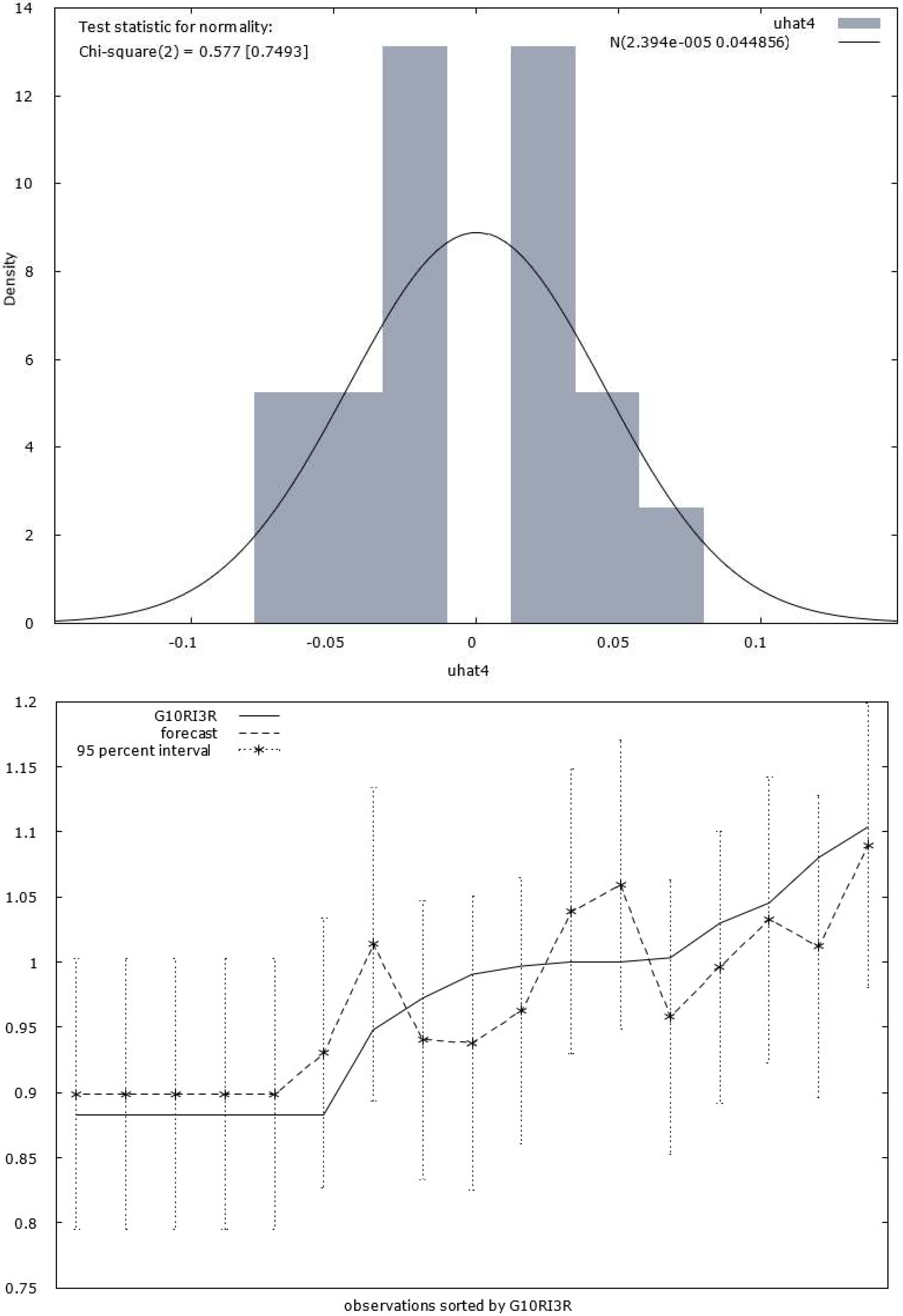
“Relative median at-risk-of-poverty gap” represents the indicator with a statistical representativity of 0.998, a value for test F close to 0, but lower than those of the above two indicators. The error is normally distributed for the Chi-square statistical test (p-value 0.75), according to the regression model:

^G10RI3R = −0.248*G10RI3R_AVG + 0.0634*G10RI3R_S + 0.00358*G10RI3R_T + 0.887*G10RI3R_EU28						(4)
	(0.129)	(0.205)		(0.134)	(0.251)
n = 17, R-squared = 0.998
(standard errors in parentheses)

The statistical tests support the model homogeneity (

Table 3. OLS, using observations 1–17. Dependent variable: G10RI3R.

	Coefficient		Std. Error		t-Ratio	p-Value
G10RI3R_AVG	−0.247844		0.129495		−1.9139	0.07790		*
G10RI3R_S	0.0633909		0.205176		0.3090	0.76225
G10RI3R_T	0.00358031		0.134193		0.0267	0.97912
G10RI3R_EU28	0.88749		0.250906		3.5371	0.00365		***
Mean Dependent var		0.968527		S.D. Dependent var			0.074937
Sum squared resid		0.026156		S.E. of regression			0.044856
R-squared		0.998369		Adjusted R-squared			0.997993
F(4, 13)		1989.340		p-value (F)			5.69 × 10−18
Log-likelihood		30.93147		Akaike criterion			−53.86295
Schwarz criterion		−50.53009		Hannan-Quinn			−53.53165

*, ***: The regression coefficients are proving that the probability density function is disturbed at 0.07, and the figures have medium statistical significance, better than model 1 and model 2. Test for normality of residual. Null hypothesis: error is normally distributed. Test statistic: Chi-square (2) = 0.577116. with p-value = 0.749343. Frequency distribution for uhat4, obs 1–17. number of bins = 7, mean = 2.39402 × 10^−0.05, sd = 0.0448557.

), as:

Interval Midpt	Frequency	Rel.	Cum.
<−0.054979–0.066196	2	11.76%	11.76%
−0.054979–−0.032544–−0.043761	2	11.76%	23.53%
−0.032544–−0.010110–−0.021327	5	29.41%	52.94%
−0.010110–0.012324–0.0011071	0	0.00%	52.94%
0.012324–0.034759–0.023541	5	29.41%	82.35%
0.034759–0.057193–0.045976	2	11.76%	94.12%
>= 0.057193–0.068410	1	5.88%	100.00%

Test for null hypothesis of normal distribution: Chi-square (2) = 0.577 with p-value 0.74934.

Interval Midpt	Frequency	Rel.	Cum.
<−0.054979–0.066196	2	11.76%	11.76%
−0.054979–−0.032544–−0.043761	2	11.76%	23.53%
−0.032544–−0.010110–−0.021327	5	29.41%	52.94%
−0.010110–0.012324–0.0011071	0	0.00%	52.94%
0.012324–0.034759–0.023541	5	29.41%	82.35%
0.034759–0.057193–0.045976	2	11.76%	94.12%
>= 0.057193–0.068410	1	5.88%	100.00%

Test for null hypothesis of normal distribution: Chi-square (2) = 0.577 with p-value 0.74934.

The histogram distribution and prediction diagrams on the confidence interval of 95% estimate a less homogenic distribution for the dependent variable in relation to the regression variable. An inflexion point can be found in the peak of the Gauss’ curve. As a result, a difference between normal and predicted evolutions appears in the inflexion point (see Figure 4).

Forecast evaluation statistics:

• Mean Error: 2.394 × 10^−0.05
• Mean Squared Error: 0.0015386
• Root Mean Squared Error: 0.039225
• Mean Absolute Error: 0.034448
• Mean Percentage Error: −0.15827
• Mean Absolute Percentage Error: 3.5281
• Theil’s U 0.56112
• Bias proportion, UM 3.725 × 10^−0.07
• Regression proportion, UR 9.212 × 10^−0.05
• Disturbance proportion, UD 0.99991

The same model points out that Romania faces to a deficit regarding poverty eradication (vulnerable point of 2030 Agenda). The analysis is connected to the indicator “Relative median at-risk-of-poverty gap” and concludes that Romania has the lowest trend between the eight analysed indicators.

“Gini coefficient of equivalised disposable income (G10RI4)” (

Table 4. OLS, using observations 1–17. Dependent variable: G10RI4R.

	Coefficient		Std. Error		t-Ratio	p-Value
G10RI4R_AVG	0.109292		0.149122		0.7329	0.47662
G10RI4R_S	−0.102951		0.120043		−0.8576	0.40664
G10RI4R_T	−0.458884		0.161392		−2.8433	0.01383		**
G10RI4R_EU28	1.21402		0.116812		10.3929	<0.00001		***
Mean Dependent var		0.978296		S.D. Dependent var			0.043072
Sum squared resid		0.005784		S.E. of regression			0.021093
R-squared		0.999645		Adjusted R-squared			0.999563
F(4, 13)		9156.076		p-value (F)			2.82 × 10−22
Log-likelihood		43.75850		Akaike criterion			−79.51700
Schwarz criterion		−76.18415		Hannan-Quinn			−79.18571

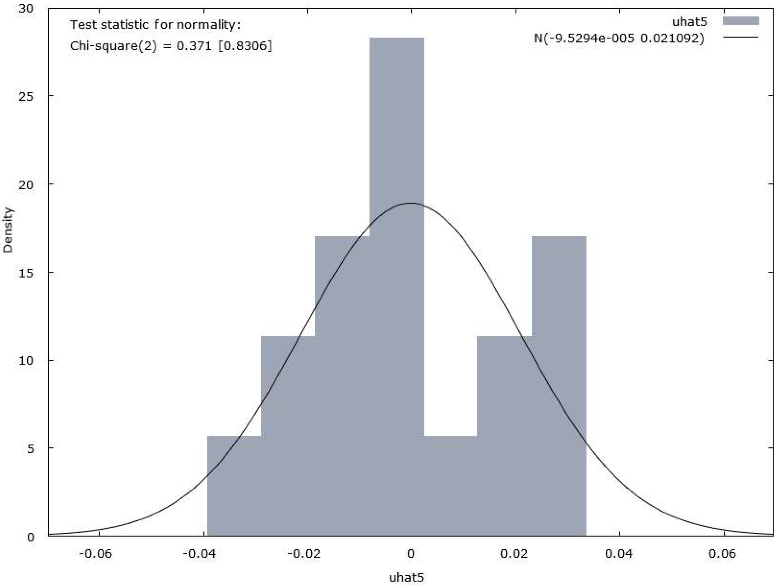
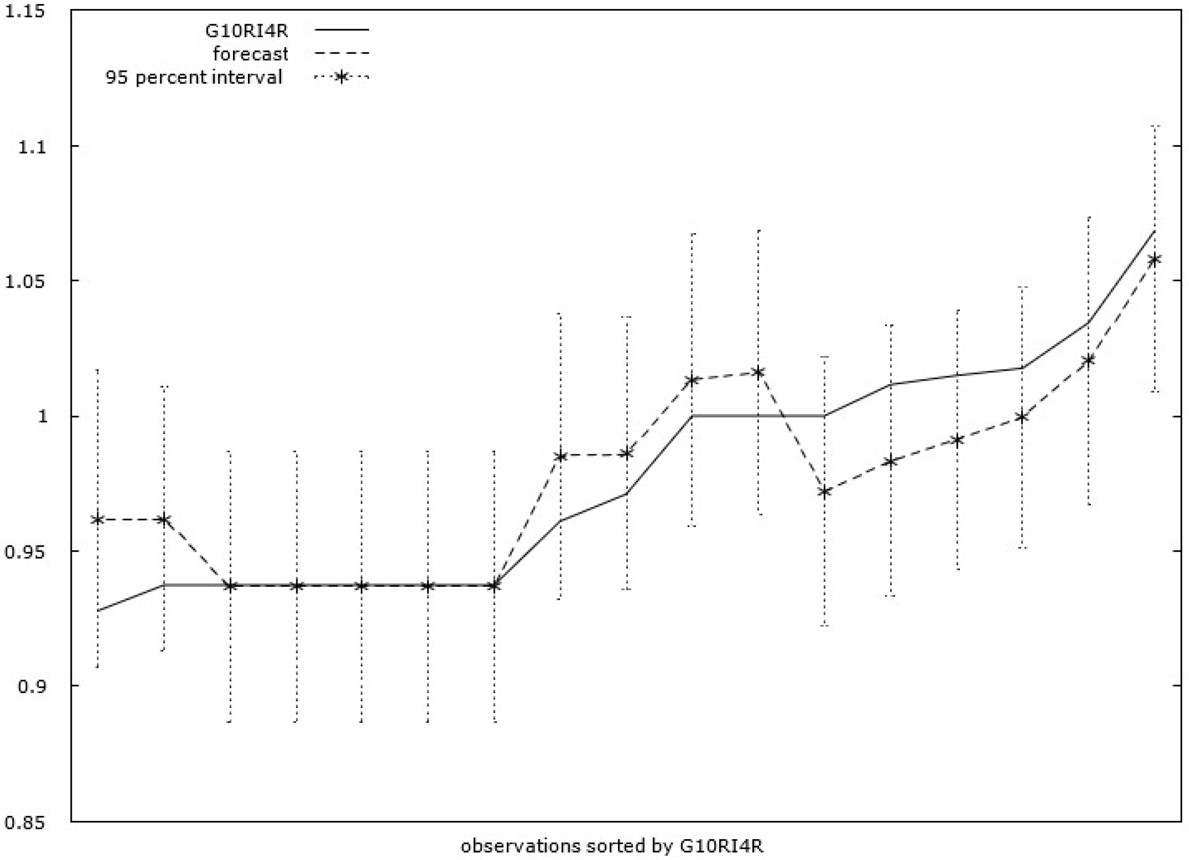
**, ***: The regression coefficients are proving that the probability density function is disturbed at 0.07, and the figures have medium statistical significance, better than model 1, model 2 and model 3. Test for normality of residual; Null hypothesis: error is normally distributed; Test statistic: Chi-square (2) = 0.371175; with p-value = 0.830616.

) supports the model in generating the greatest statistical representativity (1.0). The value for test F is close to 0, but lower than those of the above three indicators. The error is normally distributed for the Chi-square statistical test (p-value 0.83) and the model equation becomes:

^G10RI4R = + 0.109*G10RI4R_AVG − 0.103*G10RI4R_S − 0.459*G10RI4R_T + 1.21*G10RI4R_EU28						(5)
	(0.149)	(0.120)		(0.161)	(0.117)
n = 17, R-squared = 1.000
(standard errors in parentheses)

The same statistical tests demonstrate the model homogeneity, as:

The histogram distribution and prediction diagrams on the confidence interval of 95% estimate a relative homogenic distribution for the dependent variable in relation to the regression variable. An inflexion point can be found on the downward slope of the Gauss’ curve (see Figure 5).

Forecast evaluation statistics:

• Mean Error: −9.5294 × 10^−0.05
• Mean Squared Error: 0.00034021
• Root Mean Squared Error: 0.018445
• Mean Absolute Error: 0.014845
• Mean Percentage Error: −0.054589
• Mean Absolute Percentage Error: 1.5066
• Theil’s U 0.44348
• Bias proportion, UM 2.6692 × 10^−0.05
• Regression proportion, UR 0.020953
• Disturbance proportion, UD 0.97902

The model demonstrates that, under “Gini coefficient of equivalised disposable income (G10RI4)”, Romania is broadly in line with its sustainability objectives promoted by 2030 Agenda for this indicator.

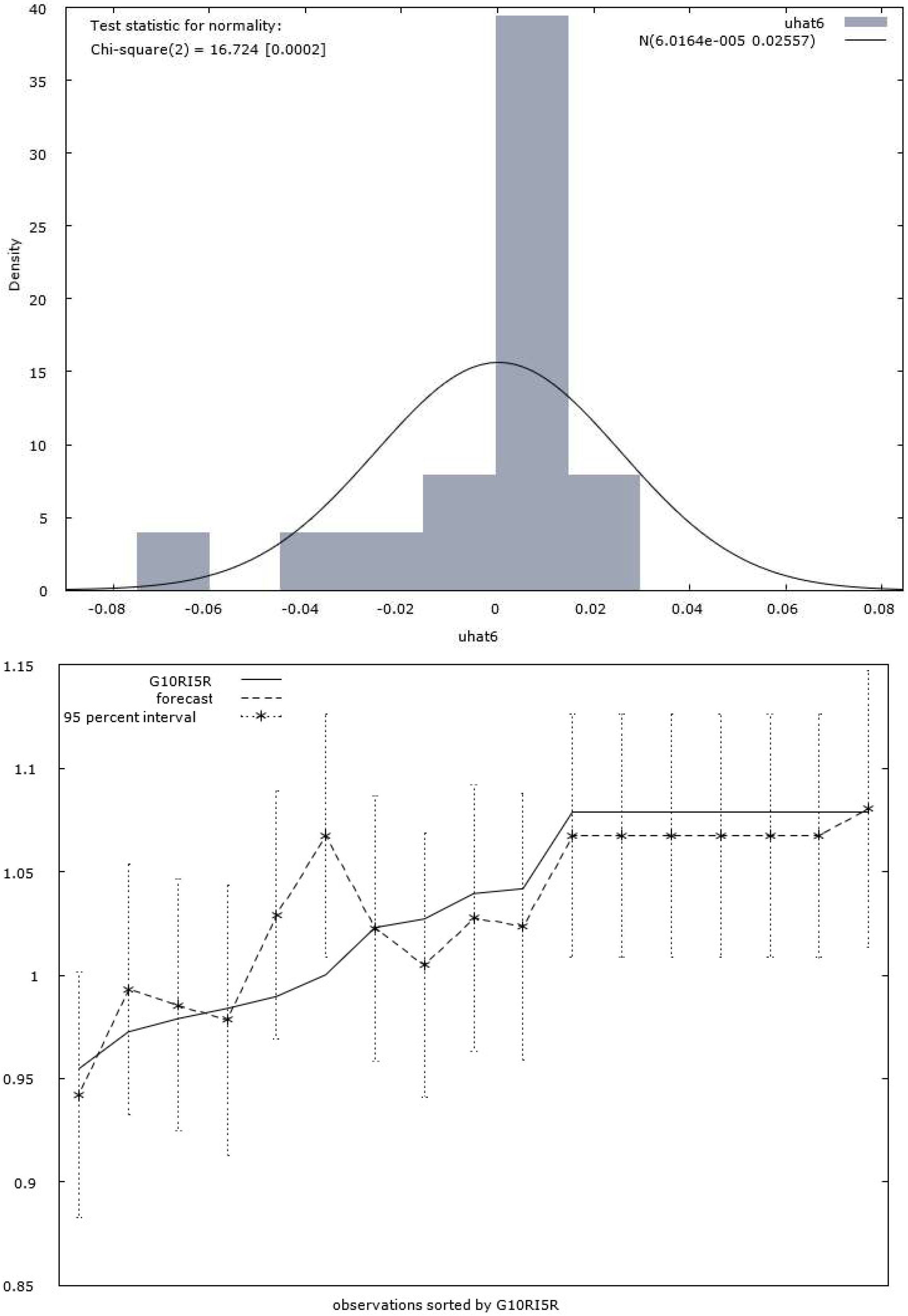
The indicator “Income share of the bottom 40% of the population (G10RI5)” (

Table 5. OLS, using observations 1–17. Dependent variable: G10RI5R.

	Coefficient		Std. Error		t-Ratio	p-Value
G10RI5R_AVG	−0.578804		0.405552		−1.4272	0.17710
G10RI5R_S	1.73042		0.769521		2.2487	0.04251		**
G10RI5R_T	−0.875702		0.249386		−3.5114	0.00383		***
G10RI5R_EU28	1.26878		0.159889		7.9354	<0.00001		***
Mean Dependent var		1.033012		S.D. Dependent var			0.045497
Sum squared resid		0.008500		S.E. of regression			0.025570
R-squared		0.999532		Adjusted R-squared			0.999424
F(4, 13)		6945.638		p-value (F)			1.70 × 10−21
Log-likelihood		40.48570		Akaike criterion			−72.97139
Schwarz criterion		−69.63854		Hannan-Quinn			−72.64010

**, ***: The regression coefficients are proving that the probability density function is disturbed at 0.04, and the figures have high statistical significance, better than model 1, model 2, model 3 and model 4. Test for normality of residual; Null hypothesis: error is normally distribute; Test statistic: Chi-square (2) = 16.724; with p-value = 0.000233572.

) leaded the model to generate a statistical representativity of 1.0 and a value for test F is close to 0 (close to the above last indicator). The error is normally distributed for the Chi-square statistical test (p-value → 0),) and the model equation becomes:

^G10RI5R = −0.579*G10RI5R_AVG + 1.73*G10RI5R_S − 0.876*G10RI5R_T + 1.27*G10RI5R_EU28						(6)
	(0.406)	(0.770)		(0.249)	(0.160)
n = 17, R-squared = 1.000
(standard errors in parentheses)

The statistical tests demonstrate once again the model’s homogeneity:

The histogram distribution and prediction diagrams on the confidence interval of 95% estimate a non-homogenic distribution for the dependent variable in relation to the regression variable. The maximum point can be found in the peak slope of the Gauss’ curve (see Figure 6).

Forecast evaluation statistics

• Mean Error: 6.0164 × 10^−0.05
• Mean Squared Error: 0.0005
• Root Mean Squared Error: 0.022361
• Mean Absolute Error: 0.016097
• Mean Percentage Error: −0.035343
• Mean Absolute Percentage Error: 1.5805
• Theil’s U 0.45396
• Bias proportion, UM 7.2394 × 10^−0.06
• Regression proportion, UR 0.004912
• Disturbance proportion, UD 0.99508

The model demonstrates the impact of the indicator “Income share of the bottom 40% of the population (G10RI5)” and explains that Romania is broadly in line with its sustainability objectives promoted by 2030 Agenda for this indicator.

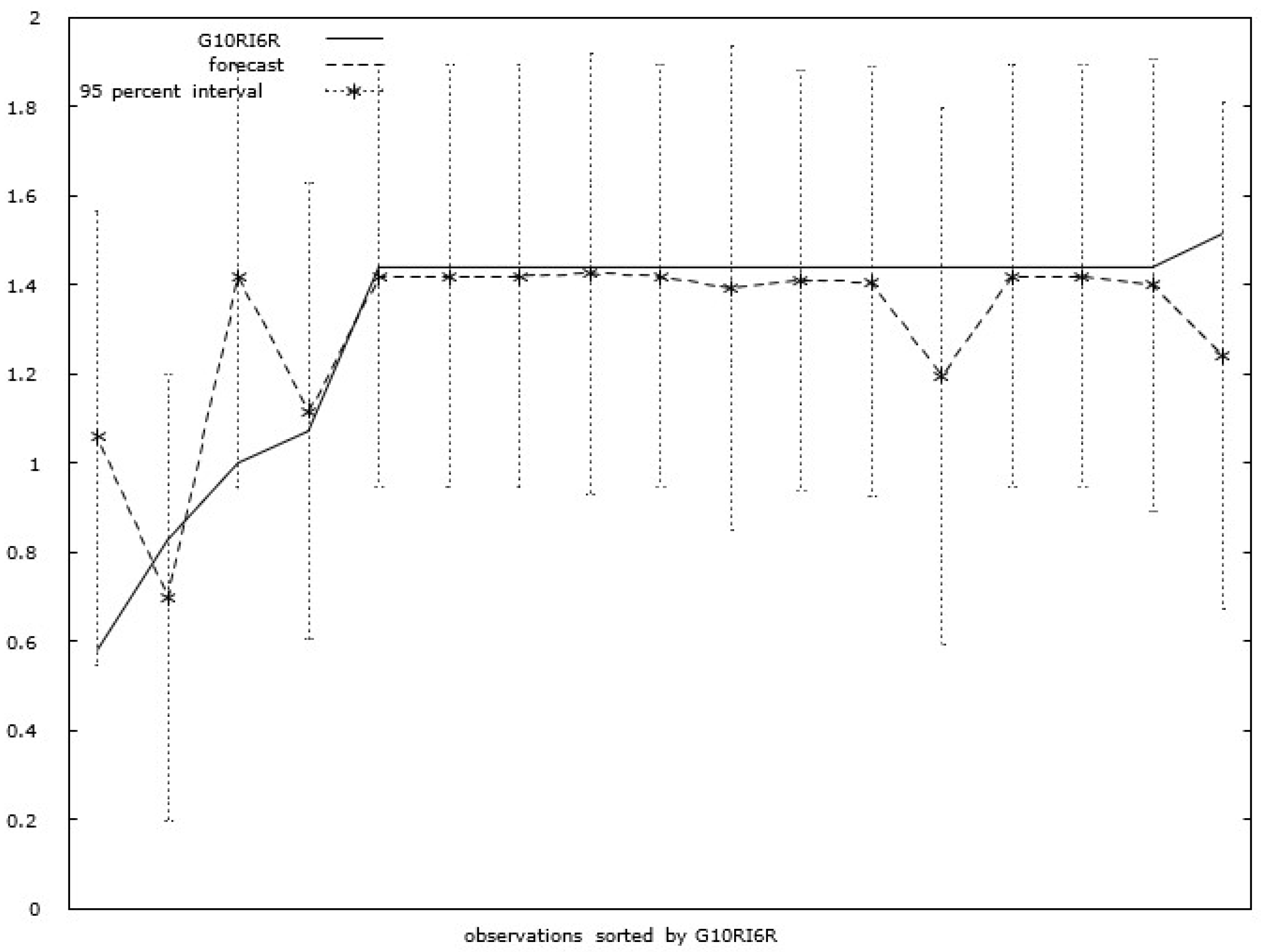
“Asylum applications by state of procedure (G10RI6)” (

Table 6. OLS, using observations 1–17. Dependent variable: G10RI6R.

	Coefficient		Std. Error		t-Ratio	p-Value
G10RI6R_AVG	−29.6835		17.6895		−1.6780	0.11720
G10RI6R_S	100.008		110.992		0.9010	0.38396
G10RI6R_T	−12.7437		76.3817		−0.1668	0.87006
G10RI6R_EU28	7.13819		5.59885		1.2749	0.22465
Mean Dependent var		1.310497		S.D. Dependent var			0.270240
Sum squared resid		0.568133		S.E. of regression			0.209052
R-squared		0.981289		Adjusted R-squared			0.976972
F(4, 13)		170.4487		p-value (F)			4.33 × 10−11
Log-likelihood		4.766250		Akaike criterion			−1.532500
Schwarz criterion		1.800353		Hannan-Quinn			−1.201208

Test for normality of residual; Null hypothesis: error is normally distributed; Test statistic: Chi-square (2) = 6.91184; with p-value = 0.0315583.

) is an indicator which generated a high statistical representativity of 0.988, a value for test F is close to 0 and an error normally distributed for the Chi-square statistical test. The model equation becomes:

^G10RI6R = −29.7*G10RI6R_AVG + 100*G10RI6R_S − 12.7*G10RI6R_T + 7.14*G10RI6R_EU28						(7)
	(17.7)	(111)		(76.4)	(5.60)
n = 17, R-squared = 0.981
(standard errors in parentheses)

The model’s homogeneity is demonstrated by the statistical tests as:

The histogram distribution and prediction diagrams on the confidence interval of 95% estimate a non-homogenic distribution for the dependent variable in relation to the regression variable, but with collinearity on the trend evolution (see Figure 7).

Forecast evaluation statistics

• Mean Error: 0.00055058
• Mean Squared Error: 0.03342
• Root Mean Squared Error: 0.18281
• Mean Absolute Error: 0.11133
• Mean Percentage Error: −3.3529
• Mean Absolute Percentage Error: 11.794
• Theil’s U 0.36884
• Bias proportion, UM 9.0706 × 10^−0.06
• Regression proportion, UR 0.00042345
• Disturbance proportion, UD 0.99957

The above model demonstrates the analysed phenomenon for the indicator “Asylum applications by state of procedure (G10RI6)” and points out that Romania covers very well the sustainability objectives promoted by 2030 Agenda for this indicator.

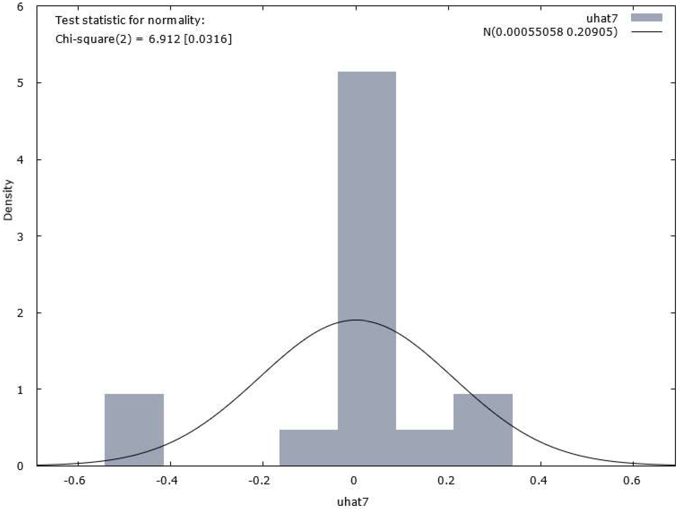
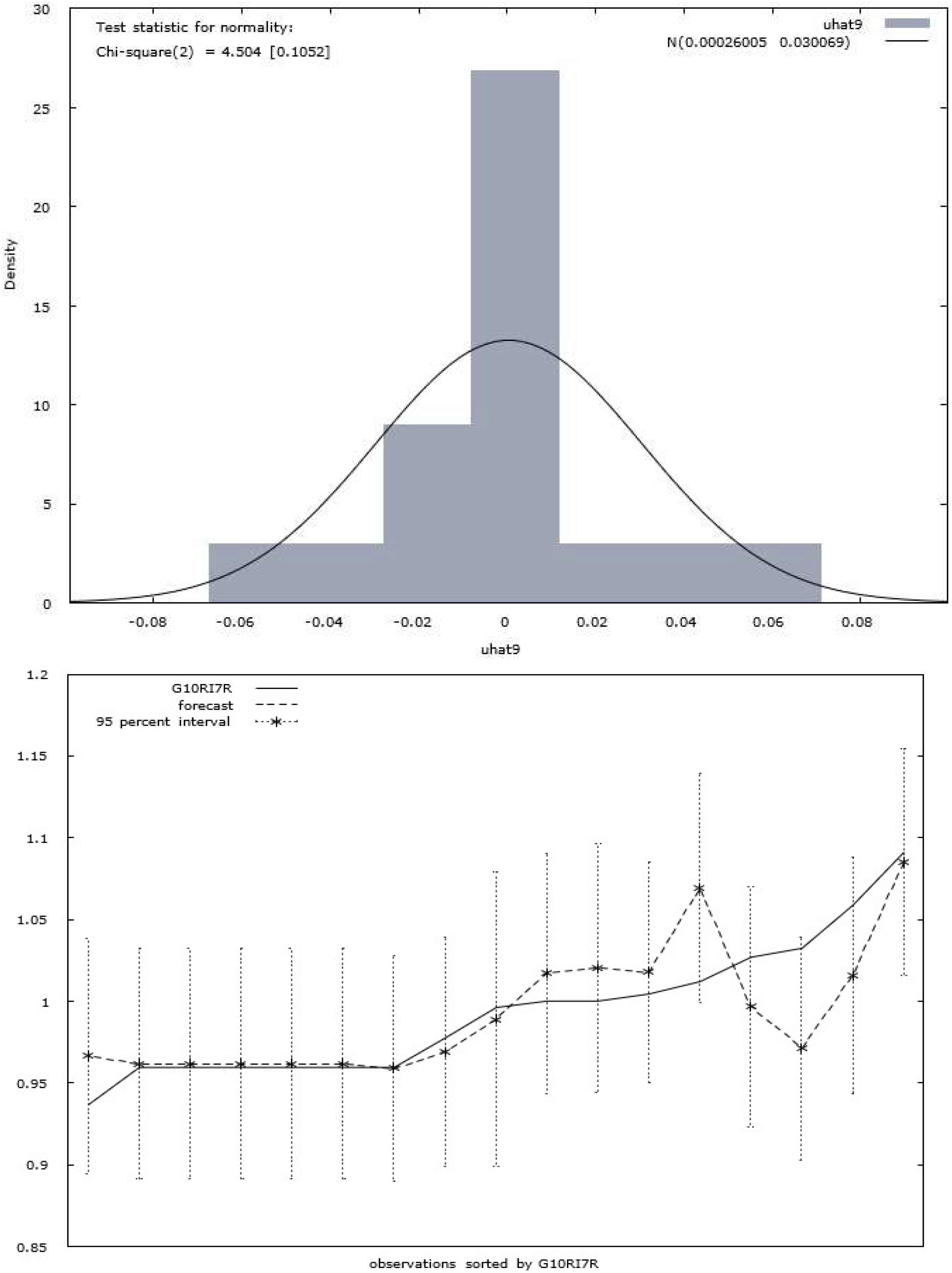
A good statistical representativity (0.999) was generated for the indicator “People at risk of income poverty after social transfers (G10RI7)” (

Table 7. OLS, using observations 1–17. Dependent variable: G10RI7R.

	Coefficient		Std. Error		t-Ratio	p-Value
G10RI7R_AVG	−0.0436021		0.0578854		−0.7532	0.46472
G10RI7R_S	0.0922207		0.0791378		1.1653	0.26483
G10RI7R_T	−0.141988		0.0411692		−3.4489	0.00432		***
G10RI7R_EU28	0.779123		0.102181		7.6250	<0.00001		***
Mean Dependent var		0.993632		S.D. Dependent var			0.041477
Sum squared resid		0.011755		S.E. of regression			0.030071
R-squared		0.999301		Adjusted R-squared			0.999139
F(4, 13)		4644.728		p-value (F)			2.32 × 10−20
Log-likelihood		37.72975		Akaike criterion			−67.45950
Schwarz criterion		−64.12665		Hannan-Quinn			−67.12821

***: The regression coefficients are proving that the probability density function is disturbed at 0.01, and the figures have high statistical significance. Test for normality of residual; Null hypothesis: error is normally distributed; Test statistic: Chi-square (2) = 4.50435; with p-value = 0.10517.

). The value for test F is close to 0 and the error is normally distributed for the Chi-square statistical test. The model equation becomes:

^G10RI7R = −0.0436*G10RI7R_AVG + 0.0922*G10RI7R_S − 0.142*G10RI7R_T + 0.779*G10RI7R_EU28						(8)
	(0.0579)	(0.0791)		(0.0412)	(0.102)
n = 17, R-squared = 0.999
(standard errors in parentheses)

The model’s homogeneity is supported by the statistical tests as:

The histogram distribution and prediction diagrams on the confidence interval of 95% estimate a non-homogenic distribution for the dependent variable in relation to the regression variable. The accumulation is achieved at the maximum point of the Gaussian curve but with collinearity on the trend evolution (see Figure 8).

Forecast evaluation statistics

• Mean Error: 0.00026005
• Mean Squared Error: 0.00069148
• Root Mean Squared Error: 0.026296
• Mean Absolute Error: 0.018066
• Mean Percentage Error: −0.016463
• Mean Absolute Percentage Error: 1.786
• Theil’s U 0.59141
• Bias proportion, UM 9.7796 × 10^−0.06
• Regression proportion, UR 0.066814
• Disturbance proportion, UD 0.93309

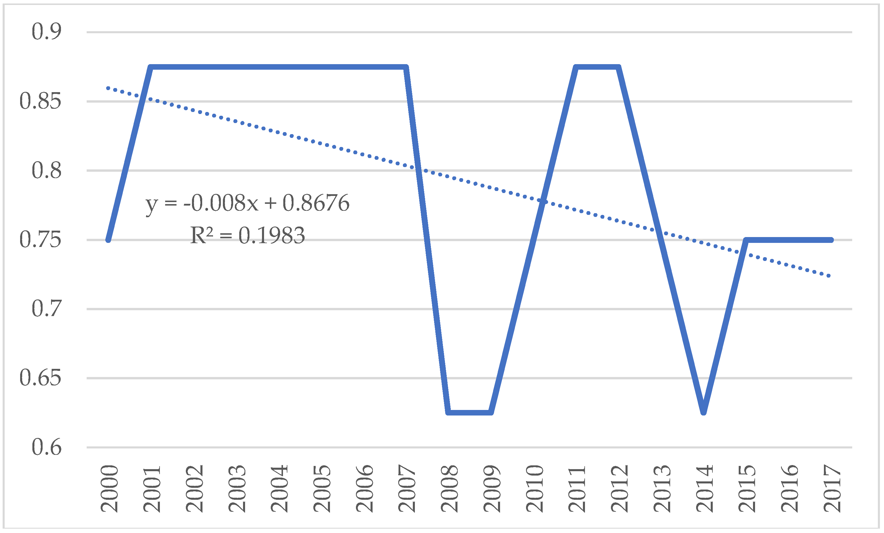
The model demonstrates the impact of the indicator “People at risk of income poverty after social transfers (G10RI7)” and explains that Romania is not broadly in line with its sustainability objectives promoted by 2030 Agenda for this indicator.

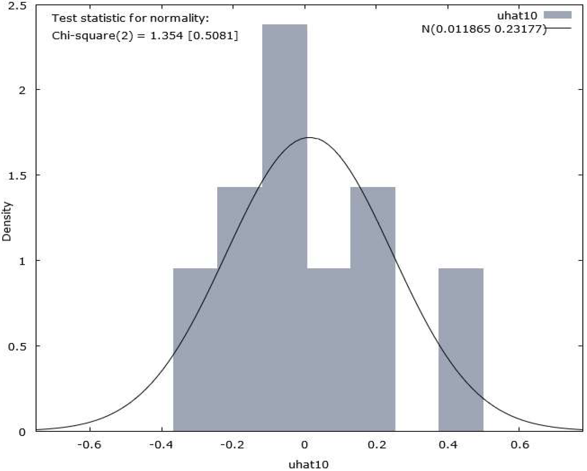
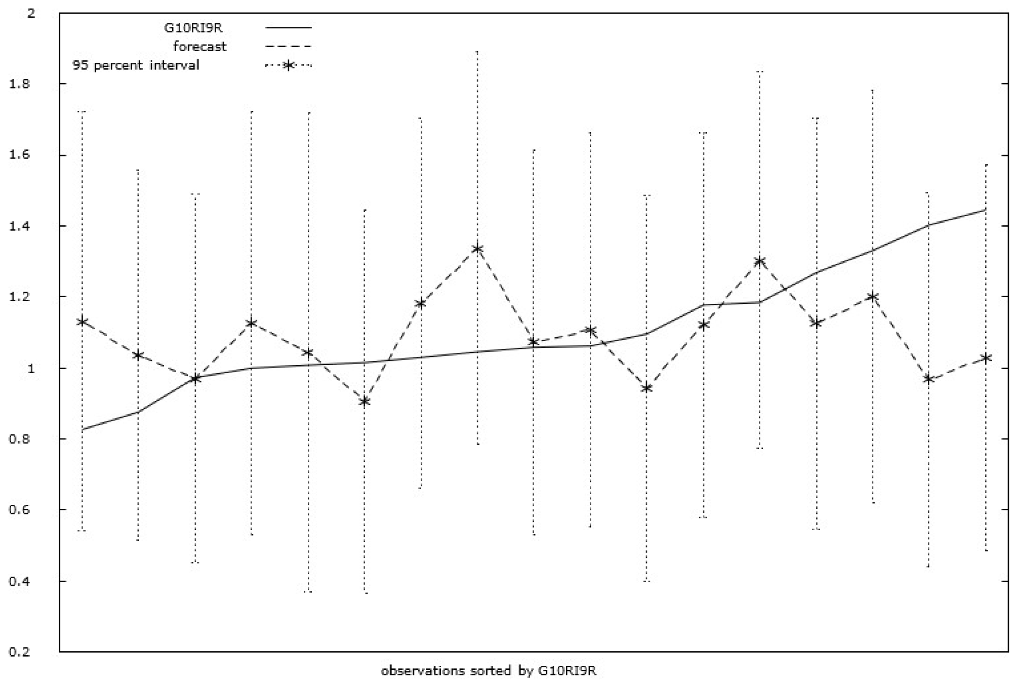
“EU imports from developing countries by country income groups (G10RI9)” (

Table 8. OLS, using observations 1–17. Dependent variable: G10RI9R.

	Coefficient		Std. Error		t-Ratio	p-Value
G10RI9R_AVG	−28792.3		599369		−0.0480	0.96242
G10RI9R_S	0.544656		0.161294		3.3768	0.00496		***
G10RI9R_T	−0.407643		0.240826		−1.6927	0.11433
G10RI9R_EU28	417604		8.69085 × 100.6		0.0481	0.96241
Mean Dependent var		1.106399		S.D. Dependent var			0.173861
Sum squared resid		0.700697		S.E. of regression			0.232163
R-squared		0.967094		Adjusted R-squared			0.959500
F(4, 13)		95.51500		p-value (F)			1.68 × 10−0.9
Log-likelihood		2.983635		Akaike criterion			2.032730
Schwarz criterion		5.365584		Hannan-Quinn			2.364023

***: The regression coefficients are proving that the probability density function is disturbed at 0.11, and the figures have medium statistical significance, better than model 1, model 2, model 3 and model. Test for normality of residual; Null hypothesis: error is normally distributed; Test statistic: Chi-square (2) = 1.35431; with p-value = 0.508061.

) represents the indicator which generated less statistical representativity (0.967), a value for test F close to 0 (p-value 0.5) and error normally distributed for the Chi-square statistical test. The model equation becomes:

^G10RI9R = −2.88 × 100.4 *G10RI9R_AVG + 0.545*G10RI9R_S − 0.408*G10RI9R_T + 4.18× 100.5*G10RI9R_EU28						(9)
	(5.99 × 100.5)	(0.161)		(0.241)	(8.69 × 100.6)
n = 17, R-squared = 0.967
(standard errors in parentheses)

The statistical tests demonstrate the model’s homogeneity, using:

The histogram distribution and prediction diagrams on the confidence interval of 95% estimate a non-homogenic distribution for the dependent variable in relation to the regression variable (see Figure 9).

Forecast evaluation statistics

• Mean Error 0.011865
• Mean Squared Error 0.041217
• Root Mean Squared Error 0.20302
• Mean Absolute Error 0.15858
• Mean Percentage Error −1.092
• Mean Absolute Percentage Error 14.129
• Theil’s U 0.81723
• Bias proportion, UM 0.0034152
• Regression proportion, UR 0.30659
• Disturbance proportion, UD 0.68999

The model demonstrates the impact of the indicator “EU imports from developing countries by country income groups (G10RI9)” and explains that Romania is broadly in line with its sustainability objectives promoted by 2030 Agenda for this indicator.

4. Discussion

The analysis of the modelling statistical data allows to represent the gaps as matrixes and to realise the risk panel regarding Romania’s sustainability on Goal 10 compared to the 4 reporting entities, according to a matrix model, as the following:

$$\mathrm{R}=\left(\begin{array}{ccc}{r}_{11}& \cdots & r_{18}\\ ⋮& \ddots & ⋮\\ r_{81}& \cdots & r_{88}\end{array}\right),$$

(10)

where: r_ij $\in$ [0, 2], 0 = sustainability, 1 = vulnerability and 2 = risk, with r_ij = 2*$\frac{G10RIR\_AVG\ast G10RIR\_UE28}{G10RIR\_S\ast G10RIR\_T}$.

The calculation of the risk coefficients is presented in

Table 9. Risk coefficients. EU: European Union, GDP: gross domestic product.

Sustainable Development Indicator under Goal 10	2000	2001	2002	2003	2004	2005	2006	2007	2008	2009	2010	2011	2012	2013	2014	2015	2016	2017	Average Risk Coefficients per Indicator for Romania
Purchasing power-adjusted GDP per capita	1	2	2	2	2	2	2	2	1	1	2	2	2	2	1	2	2	2	1.8
Adjusted gross disposable income of households per capita	2	2	2	2	2	2	2	2	1	1	1	2	2	1	1	1	1	1	1.6
Relative median at-risk-of-poverty gap	0	0	0	0	0	0	0	0	0	0	0	0	0	0	0	0	0	0	0
Gini coefficient of equivalized disposable income	0	0	0	0	0	0	0	0	0	0	0	0	0	0	0	0	0	0	0
Income share of the bottom 40% of the population	1	1	1	1	1	1	1	1	1	1	1	1	1	1	1	1	1	1	1
Asylum applications by state of procedure	1	1	1	1	1	1	1	1	1	1	1	1	1	1	1	1	1	1	1
People at risk of income poverty after social transfers	0	0	0	0	0	0	0	0	0	0	0	0	0	0	0	0	0	0	0
EU imports from developing countries by country income groups	1	1	1	1	1	1	1	1	1	1	1	1	1	1	1	1	1	1	1
Average annual risk coefficients for Romania	0.8	0.9	0.9	0.9	0.9	0.9	0.9	0.9	0.6	0.6	0.8	0.9	0.9	0.8	0.6	0.8	0.8	0.8

Source: authors’ contribution.

.

According to Table 9, there is an oscillating evolution of the annual risk mitigation regarding the sustainable development. This evolution is quantified by a trend equation as: y = −0.008x + 0.8676 (see Figure 10).

From the significance of the risks, the most significant weights belong to the indicators “Purchasing power-adjusted GDP per capita” and “Adjusted gross disposable income of households per capita”, according to Figure 11.

The above figure describes the main impact risk areas across the first quadrant. These areas are represented (above 52%) by the following: “Gross disposable income of households per capita” (24%) and “Purchasing power-adjusted GDP per capita” (28%). The other indicators in the analysis have the lowest signification risk weights, which cover 48% (see Figure 10, second quadrant).

Table 9’s transposition to the risk in

Table 10. Risk coefficients’ transposition.

Indicator	2000	2001	2002	2003	2004	2005	2006	2007	2008	2009	2010	2011	2012	2013	2014	2015	2016	2017	Average Risk Coefficients per Indicator for Romania
Purchasing power-adjusted GDP per capita	V	R	R	R	R	R	R	R	V	V	R	R	R	R	V	R	R	R	R
Adjusted gross disposable income of households per capita	R	R	R	R	R	R	R	R	V	V	V	R	R	V	V	V	V	V	R
Relative median at-risk-of-poverty gap	S	S	S	S	S	S	S	S	S	S	S	S	S	S	S	S	S	S	S
Gini coefficient of equivalized disposable income	S	S	S	S	S	S	S	S	S	S	S	S	S	S	S	S	S	S	S
Income share of the bottom 40% of the population	V	V	V	V	V	V	V	V	V	V	V	V	V	V	V	V	V	V	V
Asylum applications by state of procedure	V	V	V	V	V	V	V	V	V	V	V	V	V	V	V	V	V	V	V
People at risk of income poverty after social transfers	S	S	S	S	S	S	S	S	S	S	S	S	S	S	S	S	S	S	S
EU imports from developing countries by country income groups	V	V	V	V	V	V	V	V	V	V	V	V	V	V	V	V	V	V	V
Average annual risk coefficients for Romania	V	V	V	V	V	V	V	V	V	V	V	V	V	V	V	V	V	V

R—risk (2); V—vulnerability (1); S—sustainability (0). Variables R, V, and S represent classification coefficients and are grouped into three risk categories: first category—high risk (R—risk 2); second category—average risk (V—vulnerability 1); third category—no risk (S—sustainability 0).

is realized according to the value allocation:

The evolution in the risk table (Table 10) points out information regarding the risk trend in Romania. All nine indicators in the table belong to 10th objective from the 2030 Agenda and represent the risk presence under “Purchasing power-adjusted GDP per capita”, the risk decreases under “Adjusted gross disposable income of households per capita”, and the average risk for other indicators are as follows: “Income share of the bottom 40% of the population”, “Asylum applications by state of procedure”, and “EU imports from developing countries by country income groups”. According to the sustainability approach, Romania succeeded in having positive results for: “Relative median at-risk-of-poverty gap”, “Gini coefficient of equivalized disposable income”, and “People at risk of income poverty after social transfers”. This analysis supports further research that is able to quantify the risk sustainability impact on: GDP, Private consumption, Public consumption, Gross fixed capital formation, Exports of goods and services, and the Imports of goods and services.

5. Conclusions

The above analysis leads to the conclusion that Romania is able to decrease the disparities regarding the sustainable development, except for two indicators: “Relative median at-risk-of-poverty gap” and “People at risk of income poverty after social transfers”. On the other hand, Romania’s progress in achieving the sustainable development targets is lower than the EU average.

The general econometric model for the quantification of sustainable development that is proposed in this paper can be used for the other 16 goals from the 2030 Agenda. The model supports the decision makers in achieving a more performance management regarding sustainable development goals.

The paper succeeded in analyzing the measures proposed by the 2030 Agenda. It has an applied character by the proposed theories and models. These models were tested on significant statistical data (18 years) and different economic entities.

The authors’ scientific contributions are the following: defining a new model of analysis; demonstrating the model’s viability in a real economy; quantification of the risk impact on sustainability; and a comparative analysis between different macroeconomic entities.

The authors had equal contributions to this paper. The data used in the paper are public and official. There are no conflicts of interest between the authors and the entities analyzed in the paper. The authors respected the ethical principles during their research.

References

1. United Nations. Sustainable Development Goals. Available online: https://www.un.org/sustainabledevelopment/sustainable-development-goals/ (accessed on 27 September 2018).
2. European Commission. Next Steps for a Sustainable European Future European Action for Sustainability; COM (2016) 739 Final; Official Journal: Strasbourg, France, 2016; pp. 1–19. [Google Scholar]
3. Ming-Chuan, Y.; Qiang, M.; Sang-Bing, T.; Yi, D. An Empirical Study on the Organizational Trust, Employee-Organization Relationship and Innovative Behavior from the Integrated Perspective of Social Exchange and Organizational Sustainability. Sustainability 2018, 10, 864. [Google Scholar] [CrossRef]
4. Pinter, L.; Hardi, P.; Martinuzzi, A.; Hall, J. Bellagio STAMP: Principles for sustainability assessment and measurement. Ecol. Indic. 2012, 17, 20–28. [Google Scholar] [CrossRef]
5. Childers, D.L.; Cadenasso, M.L.; Grove, J.M.; Marshall, V.; McGrath, B.; Pickett, S.T.A. An Ecology for Cities: A Transformational Nexus of Design and Ecology to Advance Climate Change Resilience and Urban Sustainability. Sustainability 2015, 7, 3774–3791. [Google Scholar] [CrossRef] [Green Version]
6. Salvado, M.F.; Azevedo, S.G.; Matias, J.C.O.; Ferreira, L.M. Proposal of a Sustainability Index for the Automotive Industry. Sustainability 2015, 7, 2113–2144. [Google Scholar] [CrossRef] [Green Version]
7. Mekonnen, M.M.; Pahlow, M.; Aldaya, M.M.; Zarate, E.; Hoeskstra, A.Y. Sustainability, Efficiency and Equitability of Water Consumption and Pollution in Latin America and the Caribbean. Sustainability 2015, 7, 2086–2112. [Google Scholar] [CrossRef] [Green Version]
8. Schaltegger, S.; Hansen, E.G.; Ludeke-Freund, F. Business Models for Sustainability: Origins, Present Research, and Future Avenues. Organ. Environ. 2016, 29, 3–10. [Google Scholar] [CrossRef]
9. Stubbs, W.; Cocklin, C. Conceptualizing a “sustainability business model”. Organ. Environ. 2008, 21, 103–127. [Google Scholar] [CrossRef]
10. Hansen, E.G.; Große-Dunker, F.; Reichwald, R. Sustainability innovation cube. A framework to evaluate sustainability-oriented innovations. Int. J. Innov. Manag. 2009, 13, 683–713. [Google Scholar] [CrossRef]
11. Lüdeke-Freund, F.; Freudenreich, B.; Saviuc, I.; Schaltegger, S.; Stock, M. Sustainability-oriented business model assessment: A conceptual foundation. In Analytics, Innovation and Excellence-Driven Enterprise Sustainability; Edgeman, R., Carayannis, E., Sindakis, S., Eds.; Palgrave: Houndmills, UK, 2012; in press. [Google Scholar]
12. Boons, F.A.A.; Lüdeke-Freund, F. Business models for sustainable innovation: State-of-the-art and steps towards a research agenda. J. Clean. Prod. 2013, 45, 9–19. [Google Scholar] [CrossRef]
13. Fischer, L.B.; Newig, J. Importance of Actors and Agency in Sustainability Transitions: A Systemic Exploration of the Literature. Sustainability 2016, 8, 476. [Google Scholar] [CrossRef]
14. Wolfram, M.; Frantzeskaki, N. Cities and Systemic Change for Sustainability: Prevailing Epistemologies and an Emerging Research Agenda. Sustainability 2016, 8, 144. [Google Scholar] [CrossRef]
15. Geissdoerfer, M.; Savaget, P.; Bocken, N.P.M.; Hultink, E.J. The Circular Economy—A new sustainability paradigm? J. Clean. Prod. 2017, 143, 757–768. [Google Scholar] [CrossRef]
16. Barnett, M.L.; Henriques, I.; Husted, B.W. Governing the void between stakeholder management and sustainability. In Advances in Strategic Management; Dorobantu, S., Aguilera, R., Luo, J., Milliken, F., Eds.; 2018; forthcoming; Available online: https://ssrn.com/abstract=3135417 (accessed on 27 September 2018).
17. Nica, E.; Potcovaru, A.M.; Mirică, C.O. Job Loss, Unemployment, and Perceived Job Insecurity: Their Effects on Individuals’ Health and Well-Being. 2017. Available online: https://www.ceeol.com/search/article-detail?id=588752 (accessed on 27 September 2018).
18. Despotović, D.; Durkalić, D. Analysis of Budget Deficit in the Candidate Countries for EU Membership. 2017. Available online: http://scindeks.ceon.rs/article.aspx?artid=1452-48641702237D (accessed on 27 September 2018).
19. Radulescu, M.; Fedajev, A.; Sinisi, C.I.; Popescu, C.; Iacob, S.E. Europe 2020 Implementation as Driver of Economic Performance and Competitiveness. 2018. Available online: https://www.mdpi.com/2071-1050/10/2/566 (accessed on 27 September 2018).
20. Stanciu, S.; Rizea, R.D.; Ilie, A.G. Study on the Competitiveness of the Romanian Meat Processing Industry. 2015. Available online: https://www.econstor.eu/handle/10419/168981 (accessed on 27 September 2018).
Figure 1. The research process. Source: authors’ contribution.
Sustainability 10 03523 g001
Figure 2. The dependent variable in relation to the regression variable for G10RI1. Source: authors’ contribution using Gretl software.
Sustainability 10 03523 g002
Figure 3. The dependent variable in relation to the regression variable for G10RI2. Source: authors’ contribution using Gretl software.
Sustainability 10 03523 g003
Figure 4. The dependent variable in relation to the regression variable for G10RI3. Source: authors’ contribution using Gretl software.
Sustainability 10 03523 g004
Figure 5. The dependent variable in relation to the regression variable for G10RI4. Source: authors’ contribution using Gretl software.
Sustainability 10 03523 g005aSustainability 10 03523 g005b
Figure 6. The dependent variable in relation to the regression variable for G10RI5. Source: authors’ contribution using Gretl software.
Sustainability 10 03523 g006
Figure 7. The dependent variable in relation to the regression variable for G10RI6. Source: authors’ contribution using Gretl software.
Sustainability 10 03523 g007aSustainability 10 03523 g007b
Figure 8. The dependent variable in relation to the regression variable for G10RI7. Source: authors’ contribution using Gretl software.
Sustainability 10 03523 g008
Figure 9. The dependent variable in relation to the regression variable for G10RI9. Source: authors’ contribution using Gretl software.
Sustainability 10 03523 g009aSustainability 10 03523 g009b
Figure 10. The annual risk trend equation. Source: authors’ contribution using Gretl software.
Sustainability 10 03523 g010
Figure 11. Indicators’ weight regarding risks. Source: authors’ contribution.
Sustainability 10 03523 g011