Adaptive Comfort Models Applied to Existing Dwellings in Mediterranean Climate Considering Global Warming

Abstract

Comfort analysis of existing naturally ventilated buildings located in mild climates, such as the ones in the Mediterranean zones, offer room for a reduction in the present and future energy consumption. Regarding Spain, most of the present building stock was built before energy standards were mandatory, let alone considerations about global warming or adaptive comfort. In this context, this research aims at assessing adaptive thermal comfort of inhabitants of extant apartments building in the South of Spain per EN 15251:2007 and ASHRAE 55-2013. The case study is statistically representative housing built in 1973. On-site monitoring of comfort conditions and computer simulations for present conditions have been carried out, clarifying the degree of adaptive comfort at present time. After that, additional simulations for 2020, 2050, and 2080 are performed to check whether this dwelling will be able to provide comfort considering a change in climate conditions. As a result, the study concludes that levels of adaptive comfort can be considered satisfactory at present time in these dwellings, but not in the future, when discomfort associated with hot conditions will be recurrent. These results provide a hint to foresee how extant dwellings, and also dwellers, should adapt to a change in environmental conditions.

1. Introduction

In a context of scarcity of non-renewable energy sources, it is commonly acknowledged that the construction sector represents approximately one-third of the total energy consumption in the world [1]. The International Energy Agency indicates that its absolute consumption may well reach 38.4 PWh in 2040 [2], and will be responsible for 38% of the greenhouse gas emissions [3]. Considering this fact, energy efficiency in buildings has become a cornerstone in the European technical and political agenda [4], not only for newly constructed, but also for extant buildings.

The possibility that human activities are exerting a strong influence on the Earth’s climate—that is, driving climate change—has added a new factor to this debate about energy efficiency; how cities and architecture will adapt to this new reality [5], albeit with diverse uncertainties [6], stands out as one of the main focal points for research and development in the scientific community. Since the creation of the Intergovernmental Panel on Climate Change (IPCC) in 1988, which has recently published its Fifth Assessment Report (AR5) [7], a great number of studies have dealt with global warming in a variety of scientific fields, conjointly with the increase in contaminant emissions and the scarcity of resources. Several studies into future climate scenarios are based on prediction models, whose outputs morph the current available climate files [8,9,10] with future scenarios, and are valid for a number of regions around of the world.

The climatic adaption of existing buildings and their occupants plays an important role in the residential sector of Southern European countries, where most dwellings are still naturally ventilated [11].

Focusing on countries such as Spain, it can be noted that approximately 50% of the residential stock for buildings with more than 10 housing units was built before the first legislation about energy efficiency in buildings was enacted in 1979 [12] (

Table 1. Characterization of the residential stock in Spain (INE). Thousands of dwellings as a function of type of dwelling and year of construction.

Year of Construction	Detached House	Semidetached House	2-Dwelling Housing Block	3–9 Dwellings Housing Block	Over 10 Dwelling Housing Block	Buildings for Other Use	Total
After 2010	36	38	5	25	115	-	218
2006–2010	147	308	18	220	717	0	1409
2001–2005	246	370	32	299	955	2	1904
1991–2000	456	712	90	578	1417	7	3259
1981–1990	379	420	84	464	1162	4	2513
1971–1980	358	332	98	572	2059	5	3425
1961–1970	273	305	89	509	1528	4	2708
1951–1960	166	229	50	247	508	1	1202
1941–1950	102	141	28	82	126	2	481
1921–1940	115	143	30	76	138	2	504
Before 1921	243	315	54	127	109	3	852

). According to the most recent data from the Spanish bureau of statistics from 2008 [13], 57.4% of homes in the southern region of Andalusia feature air conditioners, and 84.4% of dwellings in the province of Sevilla are equipped with air conditioning devices; amongst them, 78.2% are equipped with individual air conditioners; besides, there is a relation between purchase power of households and HVAC equipment. Only 41.7% of households whose family income is less than € 1.100 have an air conditioner; these figures rise to 61.1% for households with incomes between € 1.101–1.800, 66.3% for household income between € 1.801–2.700 and 73.6% for incomes over € 2.700. In such context, previous researches show that an increase in average temperature will lead, in turn, to the implementation of active air conditioning systems in homes that previously were not equipped with these implements; this topic has been subject to discussion [11] due to the necessity of more resources to meet the building energy demand in a context of rising energy prices and fuel poverty [14]. This, as proven by data, would more affect those low-income households, which would not be able to afford nor an air conditioner, nor the energy bill associated with it. Therefore, climate adaptation of inhabitants in terms of thermal comfort is gathering attention from researchers, the aim being reducing the use of active conditioning systems and enhancing passive conditioning strategies [15] as a way to maintain acceptable levels of thermal comfort while containing energy demand and economic burden for families.

For that reason, in recent years, comfort models have been transiting from static models to what is known as adaptive comfort models [16,17], which consider occupants to inhabit naturally ventilated buildings. Amongst them, the most widespread models, which also set the foundations for building standards, are ASHRAE 55-2013 [18], and the European EN 15251 CEN (European Committee for Standardization) standard [19], with their respective reviews and studies in specific climates [20,21]; these models are based on the result from extensive fieldwork in diverse locations worldwide. Their advantage, when compared to models of static comfort, [22] relies on the fact that occupants of naturally ventilated buildings may have a wider comfort range [23] than those who are accustomed to centralized HVAC systems. In addition, current adaptive standards, which are derived from studies carried out by the RP-884 and SCATs projects, prove that indoor temperatures in naturally ventilated spaces are closely related to with the external temperatures. In particular, a variety of studies have established the relation between vernacular architecture and its surrounding environment in a way that adaptive comfort plays a crucial role [24]; besides, locally available construction materials are also important [25] and, considering adaptive comfort, even standards for zero energy buildings can be achieved [26].

However, in the current context of climate change, studying the progressive application of adaptive comfort models could have implications in the reduction of energy consumption [1], bearing in mind that an increase in the use of these models is foreseen for the near future. In this sense, dwellings in the Mediterranean climatic conditions; that is, Csa and Csb according to Köppen–Geiger classification, provide with a compelling case study. Dwellings located in Seville can be considered representative instances of them. Seville has a humid Mediterranean climate with a dry summer (Köppen–Geiger classification: Csa), though the city is located in a continental area, there is a transition zone due to the Atlantic influence. Winters are therefore humid and not very cold, while summers are dry and warm. In January the average minimum temperature is 5.57 °C, while in July the average maximum temperatures reach 36.43 °C.

Indeed, despite this climate has potential for passive conditioning of buildings, previous researches have proven that inhabitants may fall into fuel poverty not only during the cold season, but also during the warmer months [27]. The studies make emphasis on a variety of factors, amongst which the building typology and the climate are those ones exerting the most considerable influence. So that, in order to tackle with this phenomenon, a variety of researchers have focused on specific case-studies [11,28].

Spain is one of those European countries that, due to its relatively mild climate, offers great potential for reduction of the energy consumption in the building sector. The Spanish National Energy Plan predicts there will be a 15.6% general reduction in energy consumption from energy savings in the construction sector [29]. In such a way, construction standards have been updated for newly constructed buildings [30]. However, existing residential buildings, a majority of which are considered as not being well-maintained [31], fall out of the scope of this new standard. This state of affairs paints a picture of a vast building stock, built without any standard regarding energy efficiency, not being upgraded and therefore not being able to adapt to a change in climate conditions.

This research presents a case study featuring a condominium that is statistically representative of those built before 1980 in Spain (Table 1). The energy performance of such types of residential buildings has been studied in previous studies for the current climate scenario [32,33]. However, none of them have dealt with future scenarios considering a change in climate conditions.

This research strives to answer the question on how an apartment built before energy standards were mandatory is able to provide thermal comfort; the research focus on the applicability of adaptive comfort standards ASHRAE 55-2013 and EN 15251:2007 in a representative residential unit that is of the typology hereby described. Those considerations are made not only for the present time, but also for future climate scenarios per IPCC panel scenario A2. The methodology includes on-site monitoring of indoor temperatures inside a residential unit, then assessed with computer simulations; after that, the results have been extrapolated to future climate scenarios, leading to a pertinent discussion. The results of this study will help in clarifying the potentiality of the existing building stock in providing comfort per adaptive standard models, not only at present time, but also in the near future.

2. Materials and Methods

The research includes five main phases (Figure 1): The first one, denoted as ‘data collection’ aims at gathering all the necessary information to define and characterize the case study; the second one, monitoring, describes the fieldwork that was carried out in the selected case study; the third one, simulation of the model, consisted in simulating the same case study that was previously monitored; both sets of data were compared during Phase 4, validation of the model; at last, Phase 5 describes how, once the simulation model was validated, future climate scenarios were simulated. After Phase 5, pertaining conclusions are drawn regarding the applicability of the adaptive comfort models.

2.1. Data Collection

The following data, which was necessary to define the case study, was gathered considering the following categories.

2.1.1. Building Typology

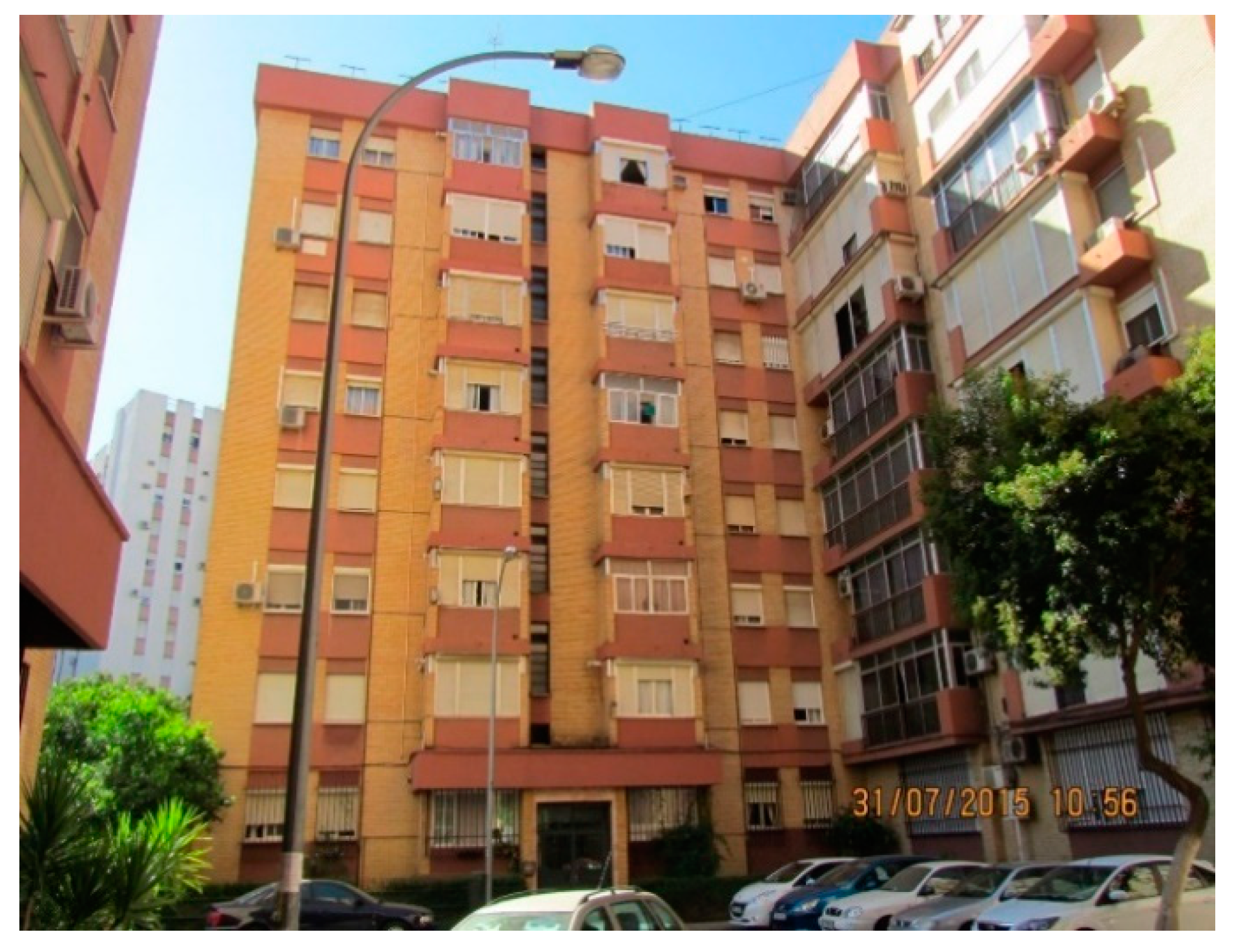
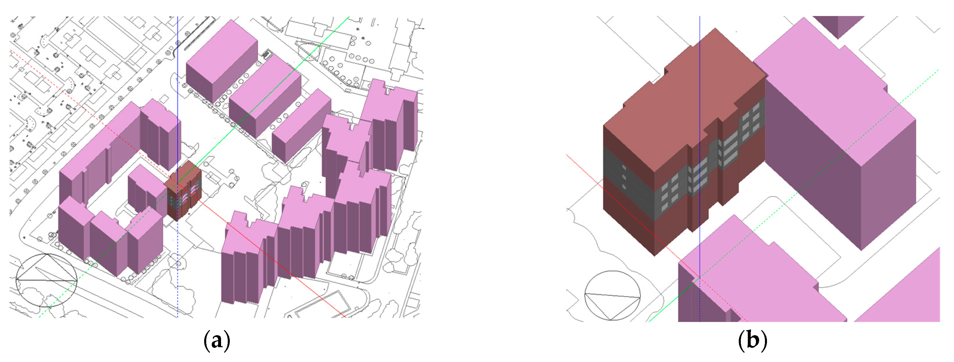
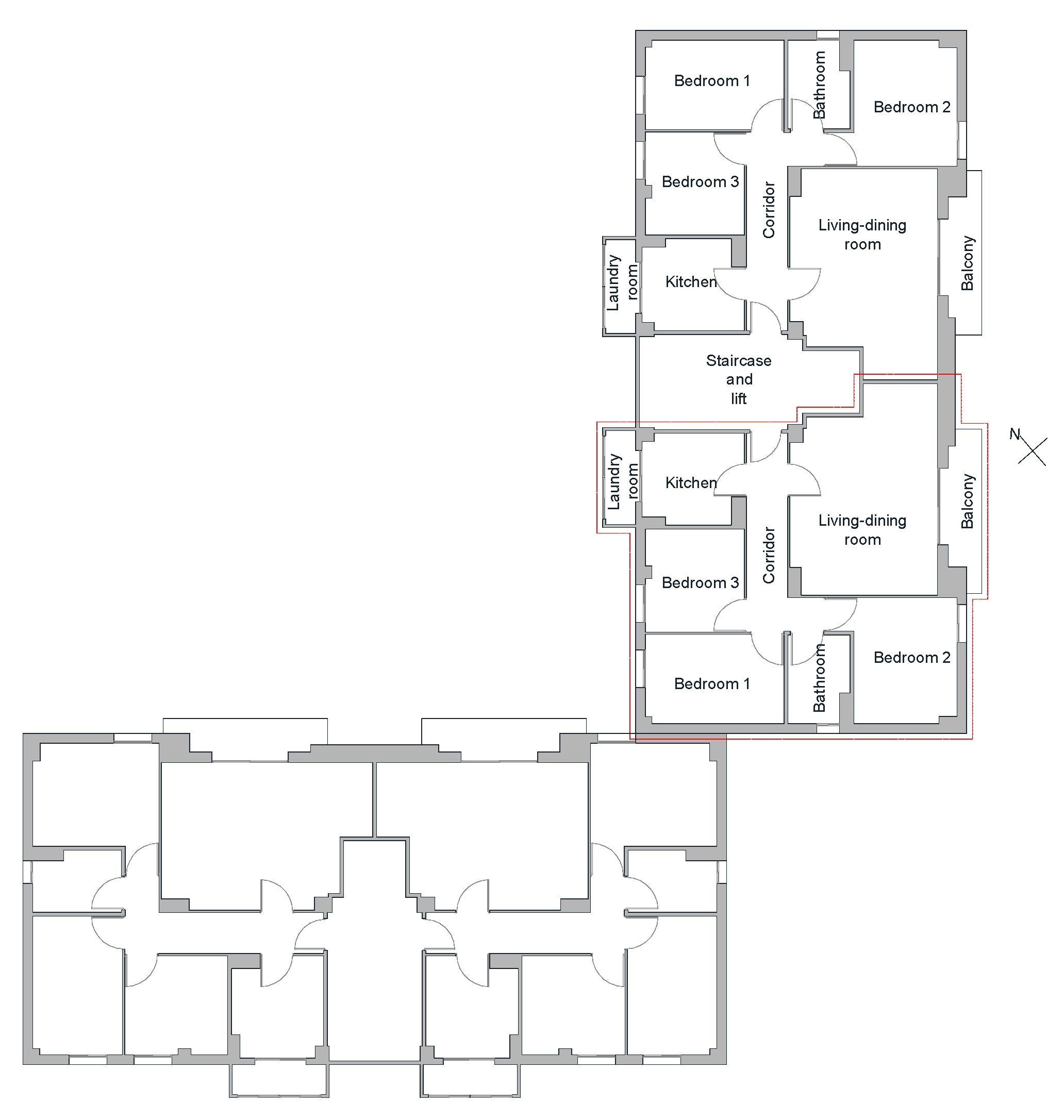
The apartment unit taken as a case study belongs to the fourth floor of an apartment building (Figure 2), built in 1978, located in a neighborhood called El Tardón, in the West district of Seville. This typology is statistically representative of the great number of dwellings that were built during the period of expansion of the city, from the 1960s to the 1980s, during which 35.5% of the actual building stock of the city was built. The floor plan (Figure 3) is similar to the most common floor plan of linear housing blocks built within that period [34]. This process was not a particularity of Seville, but common place in the majority of Spanish capital cities. According to the Population and Housing Census of 2011 [35], the typical housing type varies between 76 m² and 90 m². Further, according with data from the Spanish Statistical Office shown in

Table 2. Characterization of the residential stock in Spain (INE). Thousands of dwellings as a function of dwelling area and year of construction.

Construction Year	Area (m2)
	Total	<30	30–45	46–60	61–75	76–90	91–105	106–120	121–150	151–180	>180
Total	18,473	32	491	1925	3394	5121	2523	1822	1455	719	991
After 2010	218	1	14	24	37	56	23	14	17	10	24
2006–2010	1409	1	38	134	236	361	207	121	128	79	104
2001–2005	1904	3	36	120	282	563	266	198	168	108	159
1991–2000	3259	5	61	218	453	986	478	363	321	144	231
1981–1990	2513	1	45	147	341	847	389	302	217	103	121
1971–980	3425	1	54	279	752	1047	524	353	229	83	103
1961–1970	2708	6	84	517	771	632	261	188	128	59	61
1951–1960	1202	2	50	247	256	279	120	99	70	35	43
1941–1950	481	0	24	68	78	111	66	49	40	22	22
1921–1940	504	2	33	82	86	93	63	45	46	24	31
Before 1921	852	8	50	90	103	147	126	91	93	53	91

, 5121 dwellings (that is the 27.7% of the total) in Spain have an area between those limits, and the greatest number of dwellings (1047.3) was built from 1971 to 1980. The present case study, with an area of 77 m², and built in 1973, fits within these ranges.

The apartment comprises a living-dining room, kitchen, bathroom, and three bedrooms, with the living–dining room and one of the bedrooms facing southeast, and the other two bedrooms and the kitchen facing northwest. Figure 3 represents the building whose dwelling has been studied (marked in red), and the adjacent building, but not other surrounding structures, which are depicted in Figure 6a.

2.1.2. Constructive Systems

The building features a typical skin from the South of Spain, commonly used from the 1960s to the 1980s. The most remarkable feature was the absence of thermal insulation because, as mentioned before, it would not be mandatory until 1979. The constructive properties are shown in

Table 3. Constructive features of the selected building.

Component	Description	Thickness (m)	U-Value (W/m2K)	Internal Heat Capacity (kJ/m²K)
Exterior wall	Cement plaster	0.26	1.35	80.35
	Hollow brick masonry
	Air gap
	Cement plaster
	Brick masonry facing
Interior wall	Cement plaster	0.10	2.74	39.00
	Double hollow brick masonry
	Cement plaster
Windows	Aluminum frame; simple glazing 3 mm	-	5.89	-
Floor and paving	Terrazzo paving	0.28	1.76	147.63
	Sand
	Lightweight floor slab, cast in place, with a depth of 25 cm

.

2.1.3. Operation Hypothesis

The operation hypothesis has been assembled bearing in mind the strategies and actions that are allowed per adaptive comfort model, that is, change of clothing for inhabitants and operation of windows and blinds.

The change of clothes for inhabitants is related, in the first place, with the occupancy profile. At this point, some assumptions should be made. The inhabitants are considered to be doing light-to-moderate physical activity. The apartment is inhabited by three people, university students, who move around freely around the apartment during the 24 h. The three occupants are not always at home. However, occupants are visited frequently by other person, so in the end, the dwelling is always averagely occupied by three people. The change of clothing was surveyed, and it was determined that it operated according to the occupants’ free will. The average CLO values were dependent upon the season: 0.6 for summer, 1.1 for winter, and 0.85 for spring and autumn. Regarding the operation hypothesis, the following should be remarked. Windows in the south of Spain have two layers that can be operated independently: The sliding window itself and a blind, which is usually embedded in the frame if the windows itself and can be rolled down to darken the room. During nighttime, it is common to roll down the blinds for privacy reasons and also to protect the occupants from outside noise. That is because the poor acoustic performance of both windows and external walls. During the cold season, both blinds and sliding windows are closed; during the warm season, only the blinds are rolled down and the sliding windows remain open to allow for some degree of natural ventilation.

The operation of windows was surveyed for the three occupants of the apartment in order to check when sliding windows and blind were opened or closed. A pattern of use was stablished for the three of them.

2.1.4. Internal Loads and Profile of Use

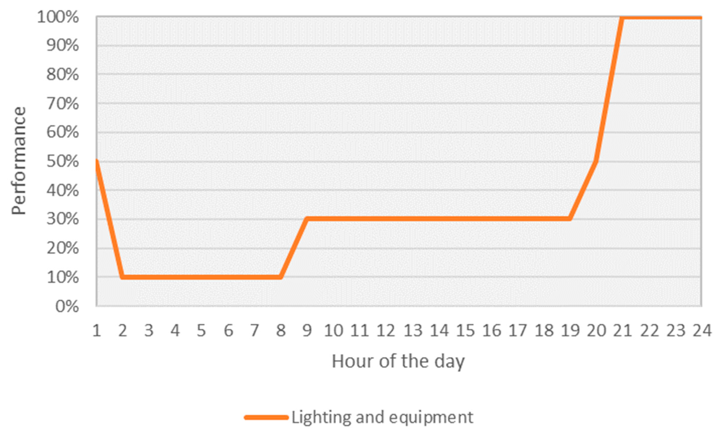
In spite of the fact that internal loads are subject to a great variation, a profile could be stablished for them, making a distinction into three groups: occupancy, lighting, and equipment. The three occupants were asked periodically about the pattern of use of lighting fixtures and electrical appliances. All unitary values used for the calculations have been taken from the ASHRAE Fundamentals Handbook.

Each occupant was considered to emit 106.6 Watts, corresponding to a light physical activity; multiplying by three occupants and dividing by the usable area of the apartment, that is 77 m², the internal load is obtained by

Table 4. Internal loads.

	Loads	Schedule
Occupancy	4.15 W/m²	Always 100%
Lighting	4.68 W/m²	According to Figure 4
Equipment	4.28 W/m²	According to Figure 4

.

The lighting fixtures of the apartment were listed, accounting for seven incandescent bulbs and two LED bulbs. About the first ones, all of them were 60 W standard incandescent bulbs, two of them located in the living-dining, one in the corridor and one in the bathroom, and the remaining three of them located in the three bedrooms; they were considered to have an efficiency ratio of 20%, that is, 80% of the consumed energy is delivered as internal heat. Therefore, these fixtures account for a total of 0.8× (60 × 7) = 336 W. The kitchen features two 40 W lighting fixtures, having an efficiency of 70%, so that the internal heat accounts for 0.3× (40 × 2) = 24 W. Considering all of them together, the internal loads due to lighting accounts for 360 W; and that, divided into the usable area of the apartment, gives a unitary lighting load of 4.68 W/m².

The equipment was also surveyed. The apartment features three computers (CPU + monitor), each one of them having a load of 110 W. Considering the three of them, the total load is 330 W, and dividing into the surface of the apartment, the final value shown in Table 4 is obtained.

In order to obtain the profile of use depicted in Figure 4, the maximum thermal load for lighting, equipment, and occupancy was calculated separately. After that, according to the considered schedule for each load, they were combined to obtain the percentage of internal loads, as a percentage of the maximum value. Regarding the schedule of the computers, they are use continuously from 21 h to 24 h because they respond to the pattern of use of the occupants, three graduate students. This profile of use was introduced also as an input parameter in the simulation model.

2.2. Fieldwork—Monitoring of Present Conditions

Previously to the actual monitoring, a dummy test was carried out for indoor and outdoor sensors to check the position where the measurements would be not altered by the effects of direct solar radiation. Besides, different positions, in relation to the occupants’ body, were tested before the final position of the indoor sensors was decided.

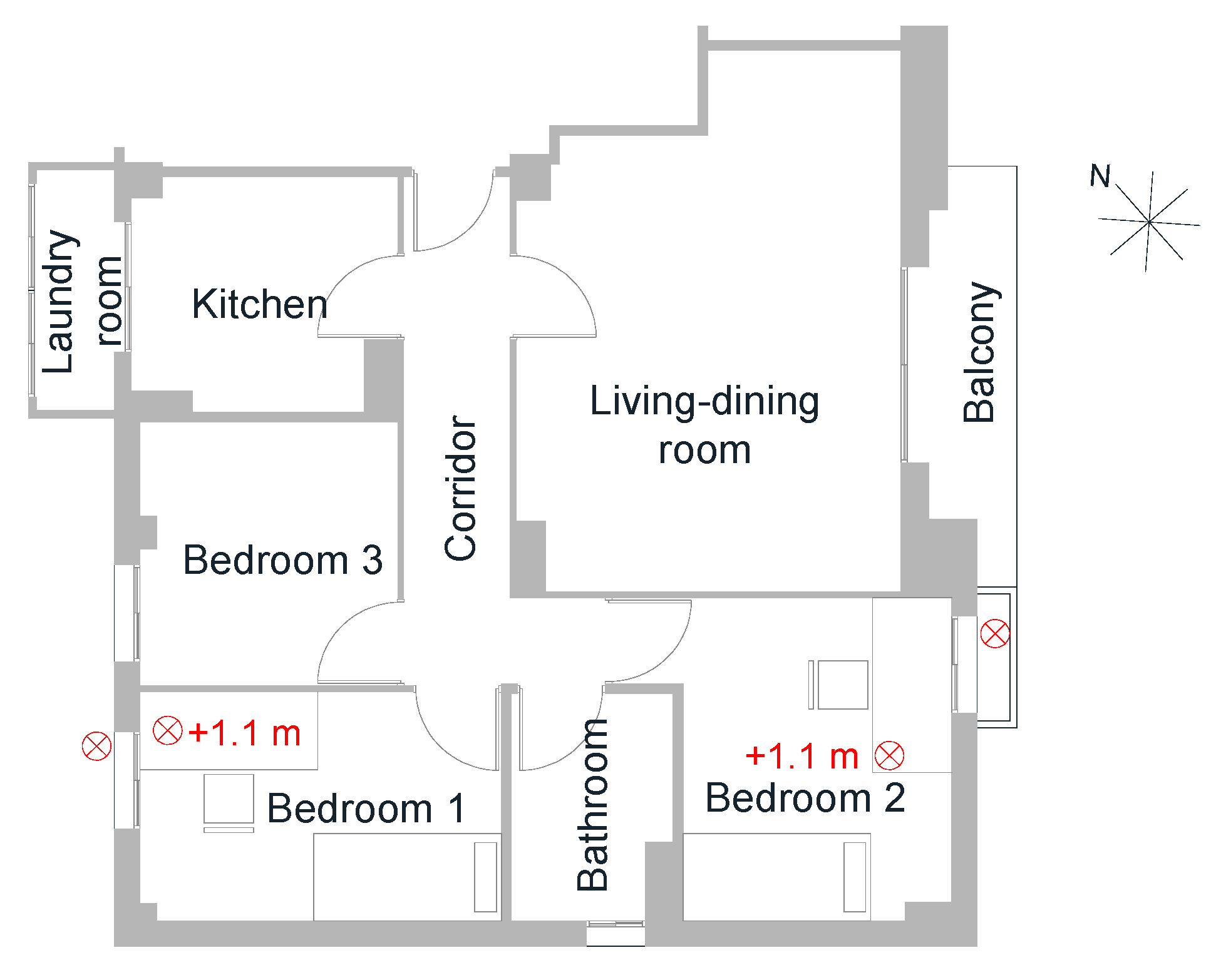
The indoor and outdoor dry-bulb temperatures (DBT) of two bedrooms were monitored during three periods: winter, summer, and spring. The durations of the monitoring periods were 21, 31, and 30 days respectively. The monitoring period was carried out by using four sensors (

Table 5. Monitoring data.

Sensor No.	Monitoring Winter	Monitoring Summer	Monitoring Spring	Location	Façade	Variable	Periodicity
01	14 Janury–3 February	22 June–22 July	14 May–12 June	Bedroom 1 indoor	Northwest	DBT	10 min
02				Bedroom 2 indoor	Southeast
03				Bedroom 1 outdoor	Northwest
04				Bedroom 2 outdoor	Southeast

), positioned inside and outside of bedrooms 1 and 2, which faced northwest and southeast façade respectively, with the purpose of avoiding problems caused by direct solar radiation. The sensor registered the dry bulb temperature in intervals of 10 min, storing a total of 39.360 measurements.

The monitoring was carried out using HOBO U12-012 sensors for indoor temperatures, and HOBO Pendant temperature/light data logger 8K-UA-002-08 sensors for outdoor temperatures, whose accuracy is ±0.7 °C. The sensors were placed following the indications of the ASHRAE Standard 55-2013 in Section 7.3.2, Physical Measurement Positions within the Building, hence, the following precautions were taken:

Since, in this case, the dwelling housed two university students, who spent most of their time studying, the indoor sensors were placed close to each occupant’s desk.

According to the furniture layout, these are zones that, in addition, are close to the windows, and that is why the foreseeable effect of the natural ventilation would be more evident.

The indoor sensors were placed facing backwards the windows to avoid direct sunlight. Bearing in mind that the occupants would remain seated most of the time, the indoor sensors were positioned at a height of 1.1 m from the floor, near the thermal node of the human body.

Outdoor sensors were placed on the underside of the windowsill to avoid direct sunlight (Figure 5).

2.3. Building Performance Simulations

Simulations were carried out as to reproduce, as accurately as possible, the actual operational conditions that were monitored in the apartment.

The apartment was modelled in DesignBuilder^®, the simulation model was assembled considering the following input data. The geometry of the model reproduces not only the apartment itself, but also the surrounding structures, modelled as obstacles, to simulate the projected shadows (Figure 6). The apartments of the upper and lower floor were also modelled to better reproduce the interaction between the adjacent thermal zones. The constructive features, internal loads, and profile of use reproduce those determined in the Section 2.2.

The climate data corresponds to Seville at current time and no HVAC equipment is considered, reproducing the actual situation of the apartment. Therefore, there are only two ways to achieve comfort per adaptive comfort model: change of clothing and operation of windows.

Change of clothing is set a parameter than can vary within the limits stablished per adaptive comfort standards, which matches data gathered on-site (0.6 for summer, 1.1. for winter, and 0.85 for spring and autumn) as per Section 2.1.3.

The operation of windows was carried out considering the ventilation was allowed when the indoor operative temperature exceeded the upper limit per adaptive comfort model standards. Designbuilder provides an option to control the natural ventilation based on the EN 15251 and ASHRAE 55 adaptive thermal comfort models. In that way, Designbuilder calculates the adaptive thermal comfort upper limit. Therefore, blinds and sliding windows were considered. Sliding windows were allowed to be opened anytime, whereas blinds were programmed to be closed from 9:30 p.m. to 8:00 a.m. every day. With regards to CLO values, considering that this study is not specifically focused on the effects of change of clothing, it was only taken into account in simulations as average fixed values observed in occupants’ behavior per Section 2.1.3.

Internal loads, reproducing the schedule that was observed according to the fieldwork, were also included in the simulation.

The modelling output data consisted on daily mean outdoor dry bulb and hourly indoor operative temperatures calculated in timesteps of 6 min (i.e., 10 simulations each hour), required to calculate respectively the weighted mean outdoor temperatures and the adaptive thermal comfort levels.

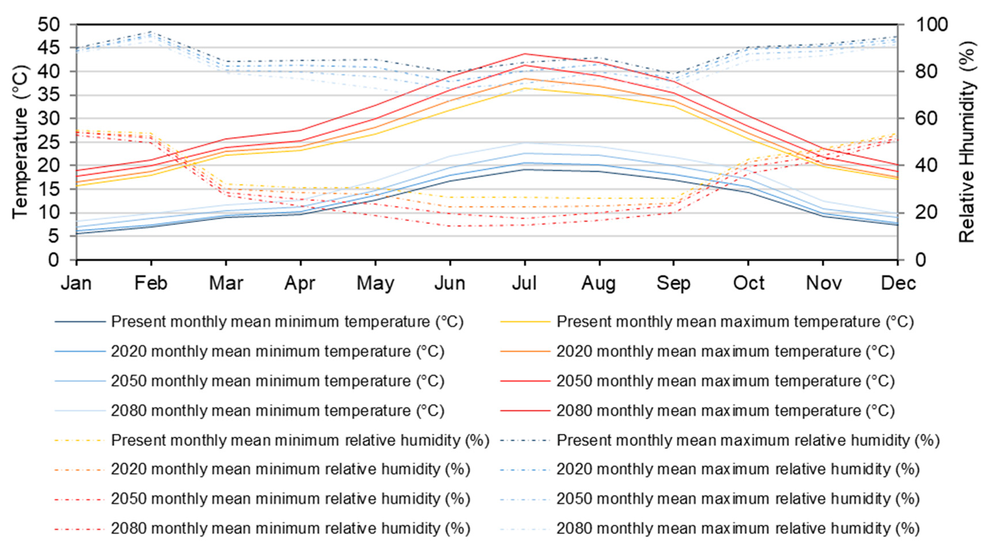
The available EnergyPlus Weather (EPW) climate file for the city of Seville, extracted from ASHRAE’s International Weather for Energy Calculations (IWEC) weather file was used to model the actual climate conditions in the simulation (Figure 7). After that, this weather file was morphed with future scenarios of climate change to predict the future climate conditions, per Hadley Centre Coupled Model 3 (HadCM3) model of the UK Met Office, which considers the combination of the A2a, A2b, and A2c guidelines. Using the CCWorldWeatherGen program [36], based on the studies of Belcher et al. [37], the present climate EPW file has been morphed with the GHG A2 scenario, obtaining three new climate files that foresee the conditions in 2020, 2050, and 2080.

According to the reliability of this method, which has already been used in previous research papers, the predicted weather data could represent those from the years 2020, 2050, and 2080 in the trend caused by climate change. However, some limitations of this method should be outlined.

Firstly, the resolution of the HadCM3 grid is mainly used in global scope, although it can be used in city or country scope. As the HadCM3 model has a grid resolution of 2.5 degrees of latitude ×3.75 degrees of longitude; that is, translated to a grid of 278 × 417 km in terms of distance in equator, or 278 × 295 km at 45 degrees of latitude, the grid is relatively greater than the objects of study.

Secondly, morphed climate files are obtained from EPW files that contain data from meteorological stations. Thus, specific environmental conditions as urban heat island or microclimate effects are not considered in these actual nor future weather data, as meteorological stations usually measure climate variables in open field spaces.

Thirdly, HadCM3 model is not able to consider extraordinary natural phenomena related with climate change as heavy seasonal floods, hurricanes, etc.

Thus, these future scenarios are considered the most likely expected mean climatic conditions in the years 2020, 2050, and 2080, in places away from the specific environmental conditions, with a margin of error according to the grid size of the HadCM3 model.

2.4. Comparison of Measured and Simulated Data and Validation of the Model

Calibration of the model was performed according to guidelines from ASHRAE Guideline 14 [38]. This guideline states that a model could be considered validated if its mean bias error (MBE) is no larger than 10%, and if the coefficient of variation of the root-mean-square error (CV(RMSE)) is not larger than 30% when the hourly data is used for the validation. The validation was based on the monitored and simulated dry bulb indoor air temperature, which was measured in 10-min intervals.

In each monitoring period, the MBE and CV(RSME) satisfied the 10% and 30% limits respectively for indoor air temperature and outdoor dry-bulb temperature (

Table 6. Model validation.

Monitoring period	Bedroom	Indoor Air Temperature		Outdoor Dry-Bulb Temperature
		MBE	CV(RMSE)	MBE	CV(RMSE)
14 January–3 February 2015	Bedroom 1	−4.71%	13.42%	4.47%	25.74%
	Bedroom 2	−6.30%	16.47%	4.61%	25.35%
14 May–12 June 2015	Bedroom 1	3.43%	7.36%	5.87%	26.26%
	Bedroom 2	4.51%	8.03%	5.46%	29.27%
22 June–22 July 2015	Bedroom 1	−0.56%	7.55%	5.93%	21.41%
	Bedroom 2	0.45%	8.42%	6.15%	23.04%

), as recommended in ASHRAE Guideline 14. That means that the outdoor dry bulb temperatures, which occurred at the same time that indoor temperatures were being measured, were similar or close to those from the EPW files. Therefore, the simulated data is considered to be reliable and there is no need to make adjustments to calibrate the numerical model. However, it should be noted that, despite being within the error limits, MBE and CV are larger during the cold season.

2.5. Simulation of Future Conditions

Taking as a base the EPW file considered for the simulation of present conditions, future scenarios for climate change have been considered. With this regard, the following points can be outlined.

Those temperatures, which are already high in summer at present time, suffer an increase by effect of climate change. Figure 7 shows the increase of monthly mean maximum and minimum temperatures as its consequences in relative humidity fluctuation. It must be understood that the temperatures mentioned in this section and shown in Figure 7 represent a likely approximation of those from the years 2020, 2050, and 2080, and therefore, according to the Hadley Centre Technical Note 44 [39], an uncertainty limit of ±5% must be assumed. In that way, monthly mean maximum outdoor dry bulb temperature in July achieves values of 38.42 ± 1.92 °C, 41.39 ± 2.07 °C, and 43.84 ± 2.19 °C, while monthly mean minimum outdoor dry bulb temperature in January increases to 6.07 ± 0.30 °C, 7.02 ± 0.35 °C, and 8.25 ± 0.41 °C by years 2020, 2050, and 2080 respectively. Thus, predictions show that temperatures are likely to not to grow in the same extent for summer and winter months, as the increases of monthly mean maximum temperatures in July and monthly mean minimum temperatures in January are 7.40 °C and 2.68 °C respectively, from present to 2080 scenario. In case of relative humidity, its trend shows some ups and downs throughout the year. Maximum and minimum monthly mean values vary from 88% to 90% and from 53% to 55% respectively, for all scenarios in January, while in July, maximum and minimum monthly mean values vary from 67% to 80% and from 14% to 26%.

2.6. Comfort Models Application—Previous Considerations

Previously to the considerations about the potential of adaptive comfort to the considered case study, the main features of the considered adaptive comfort models, in relation to the objectives of this research, are presented.

The adaptive comfort models EN 15251:2007 and ASHRAE Standard 55-2013 have been applied considering the limits established in the European standard for Category III (1, 2), as the building case of study is extant, and an acceptability of 80% for ASHRAE (3, 4). According to the Appendix I of ASHRAE Standard 55-2013, Equation (5) is known as the prevailing mean outdoor temperature, and in EN15251:2007, this is called the running mean outdoor temperature, and can be used in both standards. However, in an effort to prevent misunderstandings, hereinafter this equation will be called the weighted mean outdoor temperature. To obtain the thermal comfort limits, the weighted mean outdoor temperature was calculated for each day of the year by using Equation (5), and then, limits were calculated by using Equations (1)–(4). The number of previous days considered is seven, in accordance with both standards. The coefficient α, which controls the speed at which the weighted mean outdoor temperature responds to changes in outdoor temperatures, is considered to be 0.8, as the synoptic-scale temperature dynamics are relatively major.

$$Upper comfort limit Category III: {\mathsf{\theta }}_{imax}=0.33\ast {\mathsf{\theta }}_{rm}+18.8+4$$

(1)

$$Lower comfort limit Category III: {\mathsf{\theta }}_{imin}=0.33\ast {\mathsf{\theta }}_{rm}+18.8-4$$

(2)

$$Upper comfort limit 80\%: U_{limit 80\%}=0.31\ast {\mathsf{\theta }}_{rm}+17.8+3.5$$

(3)

$$Lower comfort limit 80\%: L_{limit 80\%}=0.31\ast {\mathsf{\theta }}_{rm}+17.8-3.5$$

(4)

$$Weighted mean outdoor temperature: {\mathsf{\theta }}_{rm}=\left(1-\alpha \right)·\left\{{\mathsf{\theta }}_{ed-1}+\alpha ·{\mathsf{\theta }}_{ed-2}+{\alpha }^2·{\mathsf{\theta }}_{ed-3}\dots \right\}$$

(5)

These models are applied on buildings without active systems, where there is easy access to operable windows, and where the occupants can adapt their clothing to the thermal conditions. Those conditions are commonly found in inhabitants of residential buildings, in which bedrooms are considered. Both models establish that the metabolic activity of the occupants must lie between 1.0 met and 1.3 met and that it is possible to adapt the clothes between 0.5 CLO and 1.0 CLO.

In addition, there are limitations in terms of the range of temperatures under which the models apply; in the case of EN 15251:2007, the weighted mean outdoor temperature upper and lower limits are set from 10 °C to 30 °C and from 15 °C to 30 °C respectively, and in the case of ASHRAE 55-2013, from 10 °C to 33.5 °C. Besides, in case of EN15251:2007, it must be considered that for weighted mean outdoor temperatures above 25 °C the graphs are based on a limited database. Under summer comfort conditions (i.e., when indoor operative temperature is above 25 °C), comfort range may be extended on the upper limit by considering increased air velocity. In case of ASHRAE Standard 55-2013, upper limit can be increased by a maximum of 2.2 °C for an average air speed of 1.2 m/s, while in the case of EN15251:2007, an increment of roughly 3.5 °C can be achieved by increasing air speed up to 1.5 m/s.

In such a way, the weighted mean outdoor temperature can be calculated by means of Equation (5), and after that the upper and lower comfort limits can be defined by means of Equations (1)–(4). The simulation model has been previously calibrated with on-site monitoring, so it can be considered as a reliable base to extrapolate the results on a yearly basis. The potential of adaptive comfort models has been tested for the present climate scenario and for three future scenarios (2020, 2050, and 2080) considering the effects of climate change.

The identification of comfort zones as well as the study of the variance of comfort balance in present and future scenarios were carried out by assessing the weighted mean outdoor temperature against indoor operative temperature.

Once the profile of temperatures was analyzed on a yearly basis, the operation of windows and blinds are analyzed and optimized in order to maximize the applicability of these models.

3. Results and Discussion

3.1. Potential Applicability of the Adaptive Comfort Models

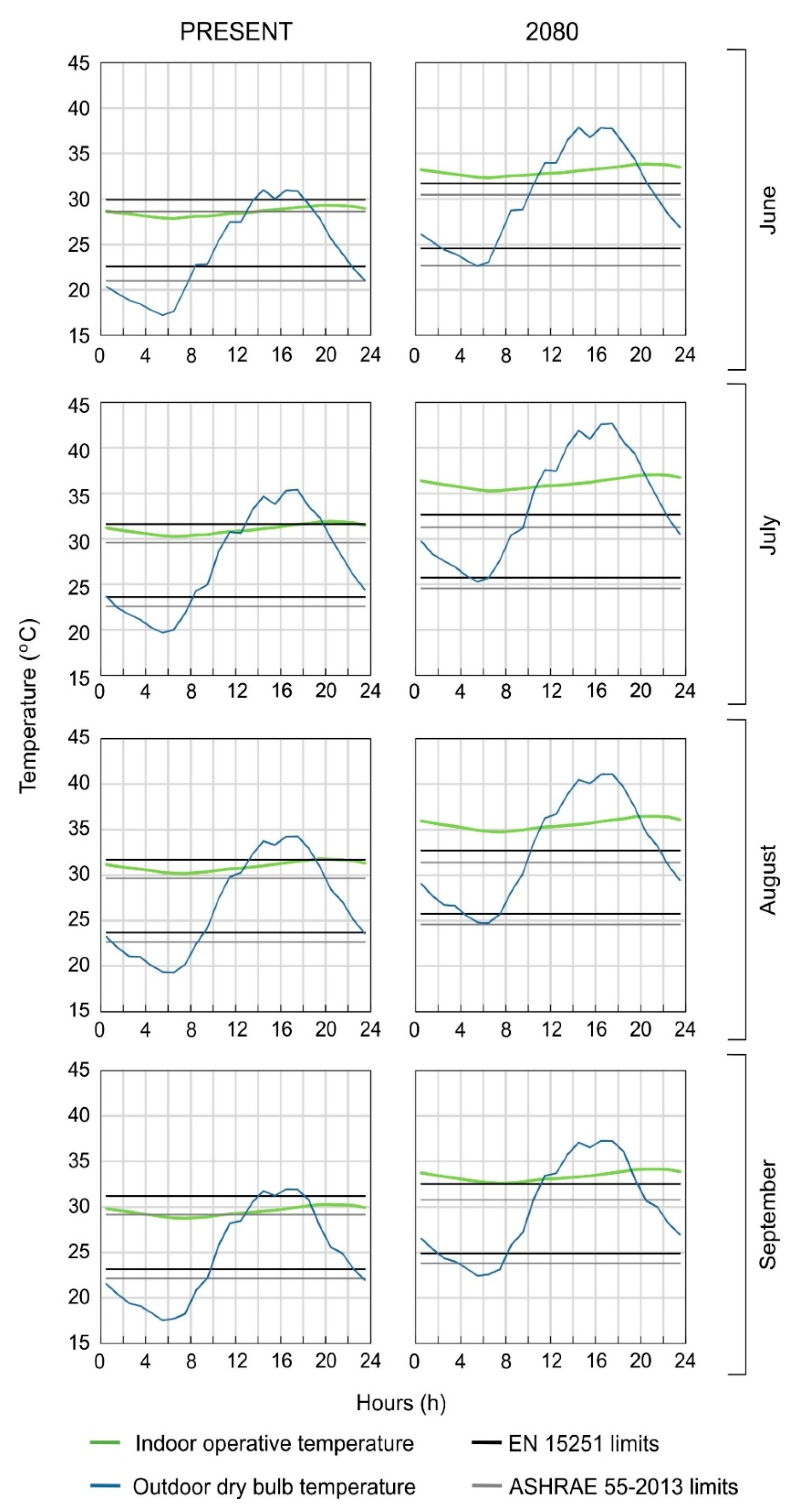
Adaptive comfort models are strongly related to the prevailing outdoor temperatures, as its application depends directly of them; results from the morphing show that, in the future, these figures will increase. According to this, discomfort is expected to be strongly related to hot conditions, rather than cold situations, significantly in future scenarios.

The predictions of future scenarios show an increment in the average annual temperature from the current 18.36 °C, to 22.74 ± 1.14 °C, as estimated for 2080. The most adverse tendency can be seen in the temperatures during the summer months. For instance, in July, the average maximum monthly temperature will increase from the current 36.42 °C to 43.83 ± 2.19 °C in 2080. In addition, the deviation of the temperatures is also commented.

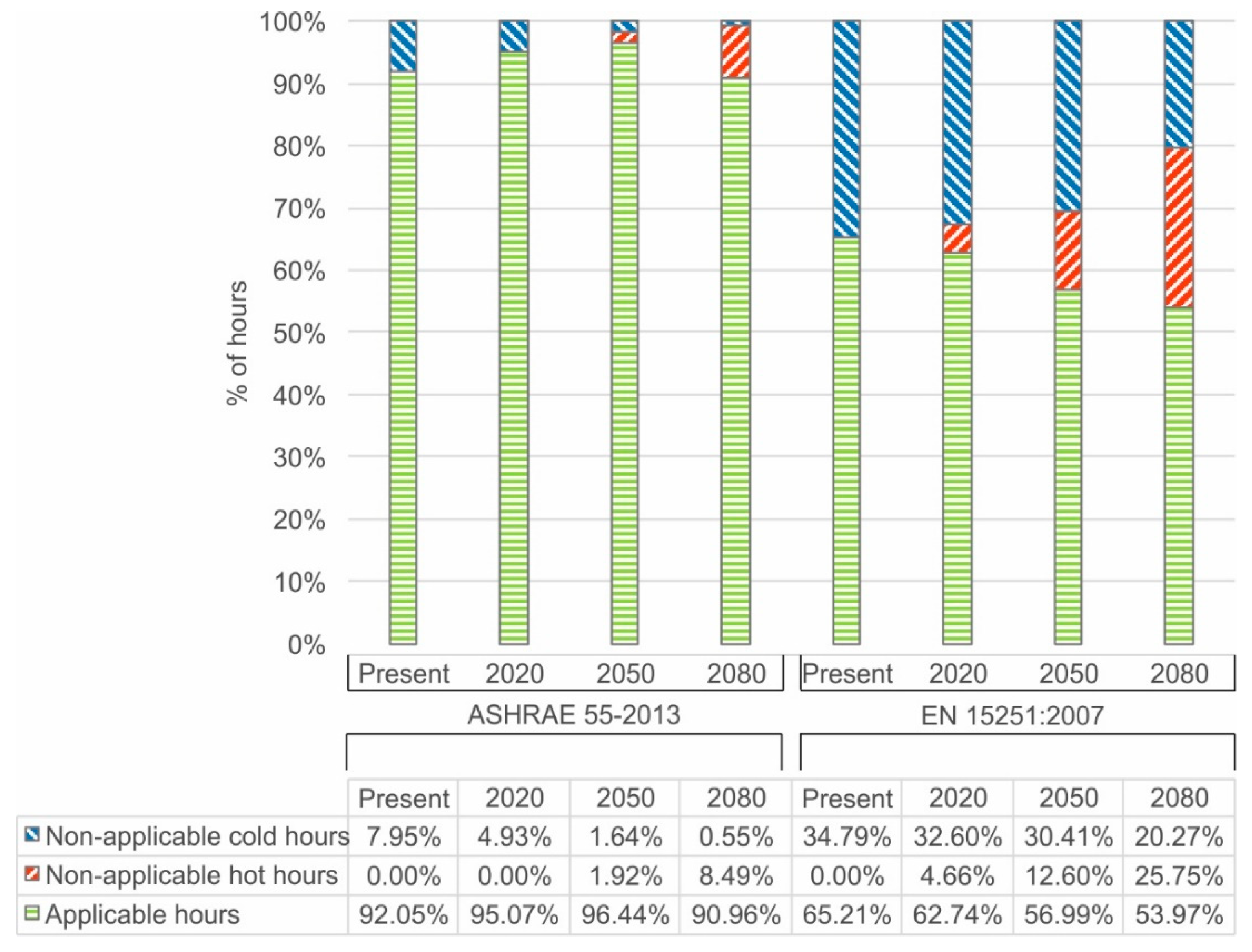
As previously stated, adaptive comfort models are only applicable between certain applicability limits regarding the weighted mean outdoor temperature. For the sake of clarity of the results, hereinafter the hours within these applicability limits are called ‘applicable hours’ (Figure 8). In the same way, the hours above and below those applicability limits are called from here on ‘non-applicable hot hours’ and ‘non-applicable cold hours’, respectively.

In the case of ASHRAE 55-2013, the percentage of applicable hours increases from the current scenario to the 2020 scenario (from 92.05% to 95.07%). This is because the temperature increases without yet reaching the limit of 33.5 °C, which implies a reduction of hours where the weighted mean outdoor temperature is below 10 °C (from 7.95% to 4.93%). In 2050 scenario, the applicable hours reach its maximum value (96.44%). However, although the percentage of non-applicable cold hours continues to fall (1.64%), the limit of 33.5 °C is exceeded (1.92%). In 2080 scenario, the increasing and decreasing trends of non-applicable hot and cold hours continue, but in greater proportion in case of non-applicable hot hours. This leads to a decrease of non-applicable cold hours (0.55%) and mainly applicable hours (90.96%).

The EN-15251 standard shows a different pattern (Figure 8). There is a smaller range of comfort at present time (65.21%) and, as different scenarios are put into play, this figure decreases until 53.97% in 2080. The trend in this case is clear; non-applicable cold hours progressively fall (from 34.79% to 20.27%) and the non-applicable hot hours increase (from 0.00% to 25.75%). In this case, the average applicable hours of all scenarios account for 59.73%, which lead to consider that application on this adaptive comfort model is limited.

There are remarkable differences between the application of the two standards. The smallest and largest differences occur respectively at present time and in 2050 scenario. At the present time, the scope of applicability of ASHRAE model is 26.84% larger than EN 15251; in 2050, this difference is 39.45%. Both models differ, in average, around 33.90% in their scope of applicability. This relatively large difference of applicable hours is due to the difference of 5 °C in the lower limit of both models (10 °C in case of ASHRAE model and 15 °C in case of EN 15251 model), and 3.5 °C in the upper application limits (33.5 °C in case of ASHRAE model and 30 °C in case of EN15251 model).

The comparison of non-applicable hot and cold hours show that winter temperatures prevails over summer temperatures in present scenario, as the non-applicable hot hours account for 0%. This balance changes with the increase of non-applicable hot hours when considering future climate scenarios.

3.2. Analysis of Weighted Mean Outdoor Temperaures Versus Indoor Operative Temperature

The potential applicability of such models gives us information about whether discomfort is expected due to hot or cold conditions. A deeper analysis is required to clarify which temperatures meet those conditions.

The aforementioned analyzed temperatures represent an average of the indoor operative temperatures simulated in bedrooms 1 and 2, with the purpose of considering the habitability conditions of the whole dwelling. Additionally, comfort hours variations between both rooms have been studied.

The applicable hours are subdivided and analyzed to differentiate between applicable hot hours (i.e., hours in which temperature is above upper comfort limit), applicable cold hours (i.e., hours in which temperature is below lower comfort limit), and comfortable hours (i.e., hours in which temperature is within comfort limits), depending on the indoor operative temperature and the comfort limits presented in Figure 9. Hereinafter, these three parameters will be known as ‘applicable hot hours’, ‘applicable cold hours’, and ‘comfortable hours’, respectively. This analysis is shown on Figure 10.

In the case of the ASHRAE 55-2013, comfortable hours increase from the current scenario (50.05%) to the 2050 scenario (56.29%), followed by a decrease in the 2080 scenario (54.85%). The percentage of comfortable hours in 2080 is higher than those at present time: that is because there is a displacement from the cold zone to the hot zone and, in that process, some hours remain stuck in the comfort zone. However, this phenomenon should not distract from the main fact: the number of hours over the comfort zone is increasing and those below the comfort zone are decreasing.

A similar situation can be seen when the EN-15251 standard is considered. A progressive decrease of the comfortable hours can be seen, similar to the decrease in the applicable cold hours. The applicable hot hours experience an increase up until 2020, and from that moment they decrease because the temperatures are so high that the model no longer remains applicable. Applicable cold hours remain negligible in all scenarios.

When analyzing the differences of the results from bedrooms 1 and 2, relatively small variations can be found. Therefore, the average of the differences in comfortable hours between both rooms in each scenario shows variations of 1.57% and 2.07% respectively in the cases of ASHRAE 55-2013 and EN15251. There are more comfortable hours in the northwest-facing room (i.e., bedroom 1) than in the southeast-facing room (i.e., bedroom 2), since the changes in temperature at night are milder than during the daylight hours as the northwest-facing room receives no direct solar radiation.

Taking a global view of both Figure 8 and Figure 9, two peculiar phenomena can be highlighted.

First, at present time there are more applicable hours in the ASHRAE 55-2013 than in the EN-15251 (92.05% versus 65.21%) (Figure 8), but there are more comfortable hours in the EN-15251 than in the ASHRAE Standard 55 (56.85% versus 50.05%). This has to do with the formulation of both models: EN-15251 is stricter when gathering hours categorized as ‘applicable comfort’ (including applicable cold and hot hours) but, inside what is called ‘comfort’ this standard is more permissive than the ASHRAE-55.

Second, the point cloud depicted in Figure 9 can be adjusted to regression lines in the form of y(x) = ax + b, a linear function. The regression coefficients of all lines are over 0.95, which indicates that the interval of confidence is acceptably high.

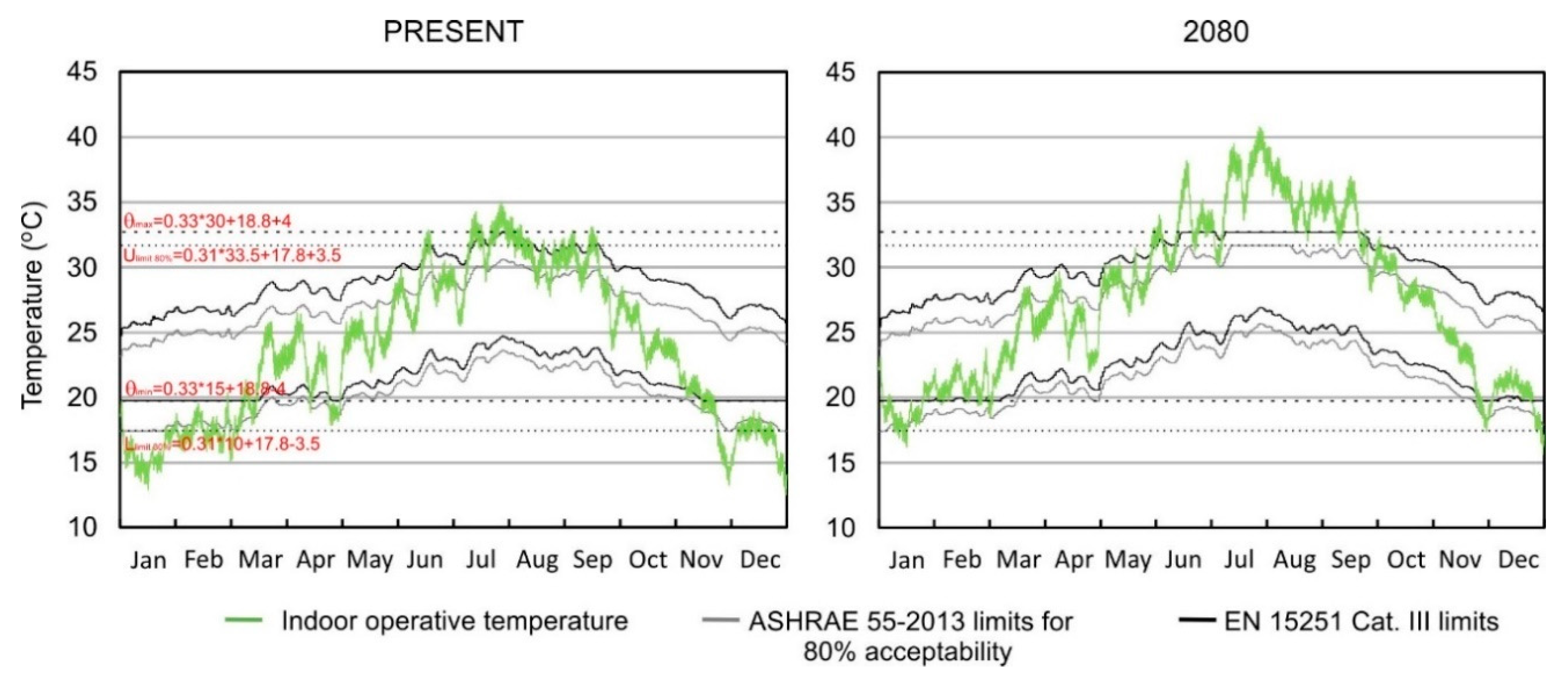
More information about this relies on Figure 10, which depicts the indoor operative temperature versus ASHRAE-55 and EN-15251 standards on a yearly basis, comparing the present scenario versus the 2080 scenario. In 2080, the weighted mean outdoor temperature clearly exceeds the upper comfort limit for both models. Besides, the temperatures below the lower comfort limit become nearly nonexistent.

This reinforces the idea previously posed in Figure 9. The increase in temperatures makes the models no longer applicable during the hot season. As an example of this, some figures can be outlined: The indoor operative temperature in summer at present time reaches a maximum value of 34.73 °C; this figure would increase up to 35.93 ± 1.80 °C in 2020, 38.22 ± 1.91 °C in 2050, and 40.50 ± 2.02 °C in 2080. At first glance, these values may seem unreal, but previous researchers have showed that in experimental rooms with no active HVAC systems located in Seville during summer, outside temperatures of around 32 °C can give indoor temperatures of nearly 40 °C inside the room [40].

3.3. Overheating Periods

The preceding discussion brings to the table the issue of overheating as the most compelling problem related to thermal discomfort, which is analyzed in this section.

Figure 11 shows that this phenomenon occurs from July to September in the present scenario, and it progressively aggravates until 2080, extending from June to the end of September; peak temperatures also become more recurring. A comparative analysis based on hourly design day of these months was carried out. Design days’ outdoor (6), indoor (7), and weighted mean (8) hourly temperatures are calculated by means of averaging the temperatures at each specific hour (e.g., by averaging the temperatures every day at 1:00 p.m., at 2:00 p.m., and so on) throughout each month.

Once the average weighted mean outdoor temperatures are obtained, the equations of the upper (1, 3) and lower (2, 4) comfort limits are applied to calculate the upper and lower comfort limits.

$$T_{a,h,out}=\frac{{{\displaystyle \sum }}_{i=1}^n{T}_{h, out}}{n}$$

(6)

$$T_{a,h,in}=\frac{{{\displaystyle \sum }}_{i=1}^n{T}_{h, in}}{n}$$

(7)

$$T_{a,h,wei}=\frac{{{\displaystyle \sum }}_{i=1}^n{T}_{h wei}}{n}$$

(8)

where $T_{a,h,wei}$ is the weighted mean outdoor temperature of the month at time h, $n$ is the number of days of the month, and $T_{h wei}$ is the weighted mean outdoor temperature at time h on each day.

Figure 11 gives a clue about the application of adaptive comfort measures. When the average outdoor temperature falls within the adaptive comfort zone, that is, below the upper limits of ASHRAE-55 and EN-1252 standards, windows should be open to allow for natural cooling. There is an additional limit for airspeed inside the building: It should not exceed 1.5 m/s as per EN15251 or 1.2 m/s as per ASHRAE Standard 55-2013.

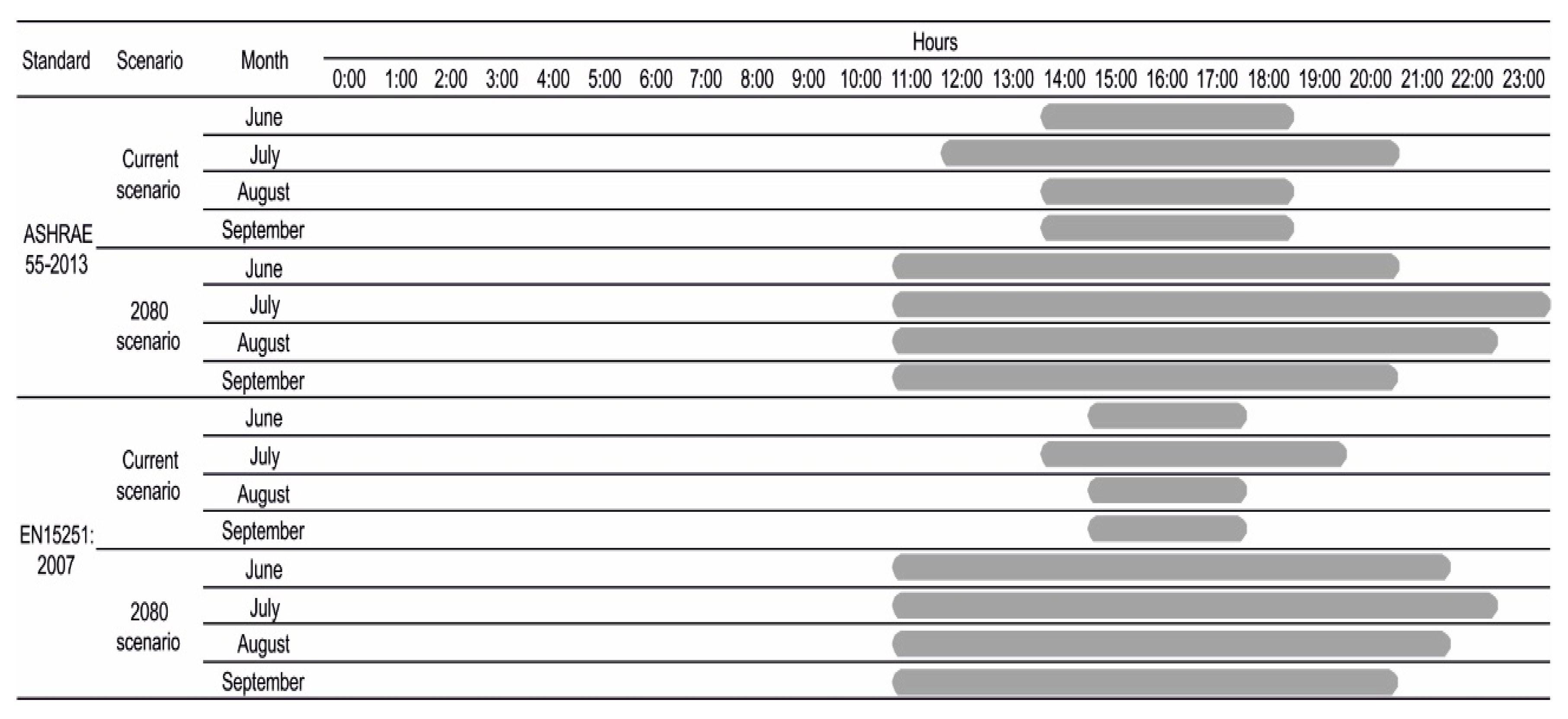
3.4. Operation of Windows

Considering the information given in the previous section, a study on the window operation schedule was carried out (Figure 12). The operation scheme considers both window opening and rolling of blinds, if possible. Windows should be open when average outdoor temperature falls within the comfort limits, on the contrary, windows should be closed, and blinds should be rolled down to protect the indoor space from excessive overheating. The grey bars represent the hours when the ensemble window-blind should be closed.

Once operation of both sliding windows and blinds was characterized during the fieldwork, these two operations were reproduced in the simulation model for the hottest period of the year. After that, the same operation was simulated considering the 2080 climate scenario in order to check how this schedule would be altered. CLO levels were allowed to vary freely, always within limits per adaptive comfort standards.

Both standards give different schedules for window operation, and EN-15251 is always stricter with this respect.

The ASHRAE model gives, at present time, a schedule for closing the ensemble window-blind with a maximum in July, from 12:00 to 6:00 p.m. In 2080, they should be closed from morning (11:00 a.m.) to nearly midnight (11:00 p.m.) so as to avoid excessive overheating. EN-12521 shows a similar pattern, but with different hours. The most unfavourable month is July (closing from 1:00 to 7:00 p.m.), so in 2080 (closing from 11:00 a.m. to 10:00 p.m.).

Those results indicate that the operation of windows remarkably vary depending on the change of climate conditions, given that occupants can freely change their clothing level within the limits of adaptive comfort standards.

4. Conclusions

This study has focused on evaluating the potential of a dwelling in providing thermal comfort considering the limits stablished by two models: the ASHRAE-55 and the EN-15251 As the adaptive comfort models focus on the consideration of human adaptation ability to changing thermal environments by means of those aforementioned actions, these could provide reductions in energy consumption, especially important in those homes that suffer fuel poverty. The case study is statistically representative dwelling that belongs to a housing building block built in 1973 in Seville, that is, before any regulations regarding building energy performance became effective. Two bedrooms with different orientations have been monitored and then simulated. This operation has been carried out not only in the present scenario, but also considering future predictions for 2020, 2050, and 2080. The study has reached the following conclusions.

Results from the monitoring assessed against those from the simulation model per adaptive comfort standards show that the models reproduce in an acceptable and accurate manner the actual conditions existing inside the case study apartment, characterized by two bedrooms. Thus, it can be concluded that both ASHRAE-55 and EN-15251 are applicable to the conditions hereby considered.

The scenarios for climate change show that the temperatures will increase, and higher peaks will be more recurrent. It has been concluded in such a way that both models will show the same tendency: the indoor operative temperatures will be displaced from the cold to the hot zone. The discomfort associated to cold conditions will be reduced and those associated with hot conditions will expand. EN-15251 will see worse conditions that the ASHRAE model, so that the latter is concluded to be more elastic to changes in environmental conditions.

Predicted indoor operative temperatures inside the considered case study will rise, placing them over the upper limit of both models. In such a way, this research gives some guidelines for future upgrades of such standards. Upper limits should be, at least, reconsidered in order to better represent the change in environmental conditions in the future

The adaptive comfort models have a limited set of strategies to regulate the temperature inside the buildings. This research has proven that, in this case, the current applicability of these models is limited. This situation will aggravate in the future. Neither proper ventilation or adaptation in clothing will be able to provide comfort in this context.

This study has also some limitations, of which the authors are aware of. The studied apartment, along with the building, are intended to be representative of the large building stock located in the South of Spain. However, only a single apartment has been studied and therefore the results should be understood as limited to this case study. So, more extensive fieldwork, considering variations in the constructive characteristics, architectonic features and patterns of occupations should be carried out in the future. In spite of that, this study is one of the first of its kind in such climatic and geographical context, paving the way for further research on this matter.

This case study, statistically representative of the building stock in the South of Spain, has been proven to be not able to adapt to a change in the outdoor conditions. Therefore, these buildings will have to resort to other strategies to provide basic levels of thermal comfort to their occupants, either by upgrading their constructive features or by implementing active HVAC systems. This opens an interesting debate and a future question for researchers about the convenience of refurbishing this large housing stock, which at present time is nearly 40 years old, or, conversely, demolishing it, making way for new homes with higher constructive standards.