
A Quantitative Assessment of LIDAR Data Accuracy


1
College of Engineering, New Mexico State University, Las Cruces, NM 88003-0001, USA
2
Department of Civil Engineering, College of Engineering, American University of Sharjah, Sharjah 26666, United Arab Emirates
3
Ministry of National Guard, Riyadh 11173, Saudi Arabia
*
Author to whom correspondence should be addressed.
Remote Sens. 2023, 15(2), 442; https://doi.org/10.3390/rs15020442
Submission received: 20 October 2022
/
Revised: 20 December 2022
/
Accepted: 23 December 2022
/
Published: 11 January 2023
(This article belongs to the Special Issue New Tools or Trends for Large-Scale Mapping and 3D Modelling)
Abstract
:Airborne laser scanning sensors are impressive in their ability to collect a large number of topographic points in three dimensions in a very short time thus providing a high-resolution depiction of complex objects in the scanned areas. The quality of any final product naturally depends on the original data and the methods of generating it. Thus, the quality of the data should be evaluated before assessing any of its products. In this research, a detailed evaluation of a LIDAR system is presented, and the quality of the LIDAR data is quantified. This area has been under-emphasized in much of the published work on the applications of airborne laser scanning data. The evaluation is done by field surveying. The results address both the planimetric and the height accuracy of the LIDAR data. The average discrepancy of the LIDAR elevations from the surveyed study area is 0.12 m. In general, the RMSE of the horizontal offsets is approximately 0.50 m. Both relative and absolute height discrepancies of the LIDAR data have two components of variation. The first component is a random short-period variation while the second component has a less significant frequency and depends on the biases in the geo-positioning system.
1. Introduction
Light Detection and Ranging (LIDAR) technology is a cost-effective, reliable, and a fast source to collect dense and accurate elevation data for many surveying and mapping applications [1,2,3]. Aerial LIDAR mapping systems are equipped with an active laser sensor, a Global Positioning System (GPS), and an Inertial Navigation System (INS) [4]. The laser sensor emits pulses at a near infrared wavelength of about 1000 nm [5]. Pulses travel through the atmosphere [6] and are reflected from ground features back to the detector. Their travel time multiplied by the speed of light is used to calculate the distance between the laser scanner and the ground [7].
Manned and unmanned LIDAR systems are widely employed in different applications including urban planning, damage assessment, natural resources, geomorphology, and archaeology [8,9,10,11,12,13,14]. The assessment of LIDAR data is becoming increasingly important in the geospatial and mapping communities. Several studies have been conducted to evaluate the quality of LIDAR data and products from such data [15,16,17].
In [18], two LIDAR datasets were acquired from about 2000 m above ground over two heavy tree coverage areas during leaf-off and snow-free seasons with an Optech GEMINI Airborne Laser Terrain Mapper. Two DEMs were then interpolated from the LIDAR datasets at one-meter ground resolution and resampled to three-, five-, and ten-meter ground resolution using mean cell aggregation. Each DEM underwent a simple low-pass smoothing filter using a mean filtering technique. Ground checkpoints were collected through total station ground surveys. Total stations have a typical accuracy of 1–3 mm ± 1–3 parts per million. Discrepancies of about 0.70 m to 2.10 m were discovered.
In [19], a Leica ALS50 Phase II was used to map an archaeological site that is ecologically and topographically diverse with alluvial terraces, foothills, mountains, and vegetation. Data were collected at 15 points/m2 ground density with flight lines overlapping more than 50%. Two control points surveyed with a Trimble R8 GNSS rover and a Trimble R7 base were used to geospatially register the LiDAR data through a 3-D shift of the LIDAR point cloud. Data were classified into bare-ground and manmade and natural features points. A Digital Terrain Model (DTM) was generated from the bare-ground points and a Digital Surface Model (DSM) was generated from all points. Results showed an average accuracy of 0.5 m for the produced DTM and DEM.
LIDAR data popularity is increasing driven mainly by the demand for 3D data for different applications ranging from 3D mapping to earth surface and city models. Common earth surface representations created from LIDAR data are the digital elevation and surface models [20,21,22]. In [23], the accuracy of LiDAR-driven DEMs interpolated from two LIDAR point clouds collected during the leaf-off season with a Leica ALS60, flying at about 3000 m above ground, for two watershed areas was evaluated. The DEMs were interpolated at one-meter ground resolution using the “LAS dataset to Raster” tool in ArcMap. Four interpolation methods in ArcMap were assessed including the inverse distance weighting and nearest neighbor interpolation techniques. Reference data were collected with a GPS ground survey. The 3-D coordinates of 45 LIDAR ground points were compared with those collected with GPS. The Root Mean Square Error (RMSE) for elevation differences between the LIDAR and GPS coordinates was 0.75 m.
In [24], the accuracy of LIDAR data collected with an Optech™ ALTM 3100 EA LIDAR sensor, flying at an average altitude of 400 m, over four sites in forestry areas was assessed. Original data was collected with an average point sampling density of 10 points/m2 then thinned to two datasets of five and one points/m2. DTMs and DSMs with a grid size of one meter were produced using the TerraScan software. Field surveys for 100 trees were conducted with differentially corrected GPS data collected with a GeoXM 2005 receiver. Mean differences and Root mean square errors (RMSEs) between LIDAR data and field surveys were about 0.10 m and 1.25 m, consecutively.
In [25], the accuracy and usefulness of point clouds obtained by Airborne Laser Scanners (ALS) and Unmanned Aerial Systems (UASs) in detecting and measuring individual tree heights were compared. ALS data were collected with a Leica ALS80-HP laser scanner over an area of 100 hectares. The average altitude during the scanning was 2700 m above mean sea level. The UAS images were collected with an RGB SONY ILCE-5000 camera mounted on a custom-built fixed wind UAS and processed in pix4D. Analysis of the discrepancies in elevation data showed that elevations measured from the ALS data were lower than those estimated from the UAS data by approximately 1.15 m with a standard deviation of about 1.95 m.
The reliability and of LIDAR data for coastal geomorphological changes was investigated [26]. Data was provided by the U.S. Geological Survey (USGS) and was collected with the Experimental Advanced Airborne Research Lidar (EAARL) sensor from 300 m above the ground. The LIDAR point cloud contained had a ground point density of 0.65 points/m2. Ground truth data consisted of 734 points and was surveyed with two Trimble R10 and one Leica GS12 geodetic GPS receivers configured for Real Time Kinematic (RTK) differential correction. In vegetated dune topography areas, dissimilarities of about 0.5 m RMSE were unveiled horizontally. However, better accuracies were attained in non-vegetated flat areas. RMSE was reduced to 0.25 m after systematic offsets between LIDAR data and ground truth were compensated for.
In [27], a point cloud obtained with a Riegl LMS-Q780 scanner, flying at an average flight height of 1240 m above mean ground, was evaluated. The point cloud had an average density of approximately 15 points/m2. Ground truth was collected with a DJI Phantom 4 Pro UAS equipped with 5472 pixels × 3648 pixels digital camera. Captured images were processed with Agisoft Metashape Professional® using structure-from-motion photogrammetric techniques. Geodetic control was established with a Leica TS02 total station. Height comparisons between the LIDAR and UAS point clouds reviled that 98% of the dissimilarities in elevations were in the range from −150 to +150 mm with an absolute maximum of 0.75 m for the whole area.
A Riegl LMS-Q560, flown at an altitude of 750 m, was employed in [28] to assess the accuracy of nine interpolation methods using cross-validation. The interpolation methods examined were Delauney Triangulation, Natural Neighbor, Nearest neighbor, Ordinary Kriging, Inverse Distance Weighted, and four spline-based interpolators. Data was collected as a point cloud with a point density of 5.13 points/m2 and a subset was held back for validation. Several DTMs were generated at 0.5-, 1.0-, 1.5-, and 2.0-meter ground resolutions. For most of the algorithms, RMSE values between 0.11 and 0.28 m were reported. Spline-based methods and the Natural Neighbor algorithm had vertical errors of less than 0.20 m for over 90 percent of validation points.
The same dataset was used in another study to map a mountainous terrain area covered by dense forest vegetation with a mixture of spruce and pine trees [29]. Ground filtering was carried out to distinguish ground points from non-ground points using the LasTools software and then manually checked. Data were resampled at different ground point densities ranging from 0.89 points/m2 to 0.09 points/m2. It was found that DTM accuracy is highly dependent on the ground point density as the RMSE ranged from 0.15 m for the 0.89 points/m2 ground point density to 0.62 m for the 0.09 points/m2 ground point density.
In [30], LIDAR data from the Golden Gate LiDAR Project was evaluated. The flying altitude was about 2500 m above mean sea level. The data minimum point density was 2 points/m2 and was filtered using TerraScan providing a set of points classified as bare-earth ground. In addition to the LiDAR data, a set of 753 points was surveyed by the USGS using the RTK differential GPS technique. The distribution of the vertical dissimilarities between the LIDAR elevation values and those observed by RTK was 19% less than 50 cm, 50% between 50 cm and 1 m, 30% between 1 cm and 2 cm, and only about 1% greater than 2 m.
From the presented literature, we can conclude that most of the previous research used GPS ground surveys to assess the quality of the LIDAR data. Despite the fact that GPS in general has higher accuracy than LIDAR data, the reliability of GPS is affected by distances to the base point, time of observation, and satellite geometry. In addition, the lack of a clear line of sight is occasionally found in urban geographic environments and this could harm the quality of the GPS signals. Therefore, in our study we used traditional ground surveying techniques, a total station, to assess the quality of the LIDAR data. Moreover, most of the previous research focused on either relative or absolute assessment of LIDAR data. In our study, we evaluated both the relative and absolute quality of the LIDAR data. The LIDAR data set was collected with an Optech LIDAR system and ground control was surveyed using conventional ground surveying techniques.
2. Data Acquisition and Dataset Characteristics
2.1. LIDAR Dataset
The data used in this research was collected in November 2014 using an Optech ALTM 3100 EA LiDAR flown at 600 m above the mean ground. Under optimal conditions, the system is capable of achieving elevation accuracies as high as ±3 cm, 2-σ at 500 m elevation, 33 kHz Pulse repetition frequency (PRF) with ±10° scan angles, [31]. The instrument operated with a scan angle of 18° and a laser pulse rate of 100 kHz. An Applanix POS/AV 510 system was co-mounted with LiDAR to record the aircraft’s 3-D position and attitude (pitch, roll, and yaw). The reported positional accuracy of the system is 0.05–0.3 meter with velocity uncertainty of 0.005 m/s, roll and pitch accuracies of 0.005°, and heading accuracy of 0.008° [32]. The accuracy of the GPS unit in RTK mode is 2 cm + 2 ppm. The reported range resolution of the lidar is 1 centimeter with a resolution of 0.01° and beam divergence of 0.1 mrad. The overlap between swaths was 30%. The point cloud on the ground had 9.54 points/m2. The data consists of fourteen strips flown in the north–south direction. Figure 1 below shows an across-band view, 500 m wide, of the fourteen strips.
Imprecision in the GPS positioning, the INS orientation, component misalignments, errors in the angle encoder and other sources of error, cause the same ground spot in two adjacent overlap strips to have two different coordinates. This leads to systematic errors in position and attitude and may produce a tilt in the resulting scanned surface. In order to reduce discrepancies between adjacent strips, we applied the mathematical model presented in [33] for strip adjustment. In this model, errors are modeled by three offsets, three rotations, and three time-dependent rotations. Tie points in adjacent strips were identified and least squares matching was applied to laser scanner data points to achieve higher relative accuracy between adjacent strips.
2.2. Reference Dataset
In order to evaluate the data set used in this research, a ground survey was conducted on an area with a large athletic area, which contains tennis courts and soccer and basketball fields representing the selected test area. The study area has two main useful characteristics. First, the area is flat and horizontal with almost no significant slope over the tennis courts or sports fields. This enables the examination of pure height accuracy because the flatness and the lack of slope of the surface rule out any planimetric uncertainty effects. Second, the presence of drainage ditches around the area facilitates the computation of planimetric accuracy.
The fieldwork was conducted by surveying 440 points using a TOPCON (GTS–303) total station. Three measurements were made for each point and the reported horizontal and vertical RMSEs were less than one centimeter. Figure 2 shows a part of the surveyed area. Those points were then used to establish the correspondence with the laser data based on the spatial positions and consequently compute the absolute accuracy.
3. Relative Accuracy of LIDAR Data
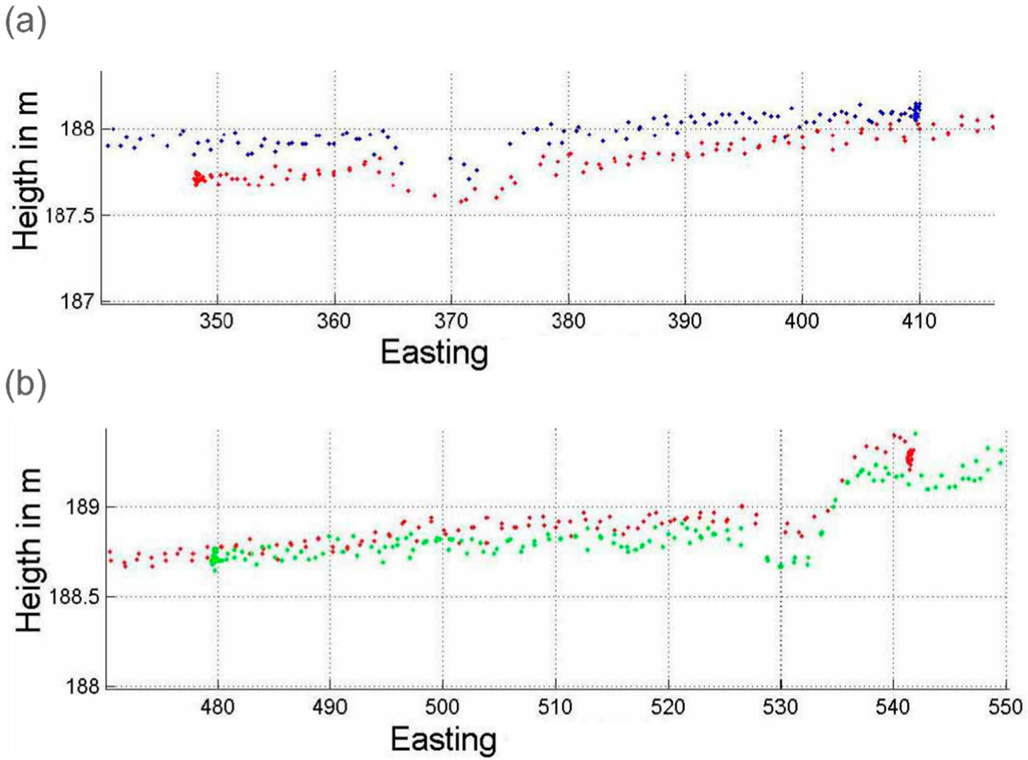
Airborne laser scanning data are acquired in a strip-wise pattern with a strip width varying depending on the chosen scan angle and the flying height. Usually, those strips are flown in parallel and overlapping until the entire region of interest has been covered. Overlap between strips, as shown in Figure 3, provides a means to verify the relative consistency between them. It is evident that imprecision in system positioning, orientation, and ranging may cause the same point to have two different heights if scanned at two different times, which always happens in neighboring overlapping data strips. These points can be considered as tie points in strip adjustment to adjust strips and eliminate or at least minimize relative error between them. However, the discrepancy between tie points from adjacent strips gives an indication of the relative offsets without any strong conclusion of the absolute error. In this section, the height discrepancy is examined between adjacent strips.
Relative Height Offset
In the test data in this research, the percentage overlap between adjacent strips was designed to be about 30% of the total swath width. A nominal swath width of 200 m would then have an overlap region on either side of 60 m. However, due to the actual conditions during the data collection, such as wind, overlap areas between strips ranged from less than 60 m to as wide as 120 m as shown in Figure 4. Since the data consists of 14 strips, 13 overlap regions were examined to quantify the relative height discrepancies. The fact that the data is dense and the overlap regions included in the testing are large increases the likelihood of having coincident and nearly coincident data points. Therefore, the relative height accuracy was obtained directly by computing the differences between such nearly coincident data points.
Three experiments were conducted during the testing. In order to minimize the effect of slope and spatial position on the collected heights, the planimetric distance between tested points was limited to be less than 0.05 m in the first test. In spite of these limitations, there were some misinterpreted differences (more than a half meter) due to the height jump between the tested points. Height jumps on building edges is one example. On building edges, two points within a few centimeters could have a great height jump since one might be on the ground and the other one is on the roof. Such outliers were detected based on the statistical interpretation of the computed discrepancy. Consequently, they were deleted from the data set to eliminate their influences. A manual examination verified the stated assumption that these outliers coincided with abrupt height transitions. Then, to include more points in the computation and strengthen the statistics, the planimetric-distance constraint was increased to include points within 0.10 m and 0.25 m. Table 1 summarizes the results for all of the 13 overlap regions with 0.05 m, 0.10 m, and 0.25 m planimetric distance allowance. However, changing the planimetric distance and including more points did not significantly change the discrepancy average in all overlap regions as shown in Table 1. This is because the planimetric distance is less than the point density. In the rest of the study, we used the 0.05 m planimetric distance allowance.
Figure 5 summarizes the behavior of the mean relative height offset between adjacent strips. As shown in Table 1, the discrepancy did not show a well-defined behavior. However, the discrepancy shows a trend with time (North–South direction) since the strips where ordered on the time they were scanned (strip 1 was the first one to scan and strip 14 was the last). In the first four overlap regions, the discrepancy was within ±0.04 m. Then, the average discrepancy between strips (5–6, 6–7, 7–8, 8–10, 10–11, and 11–12) seems to increase up to 0.10 m with a negative sign (since the discrepancy was computed by subtracting the height of the right strip from the height of the left strip). Then, in the last two overlap regions (12–13 and 13–14) the discrepancy dropped to −0.06 m.
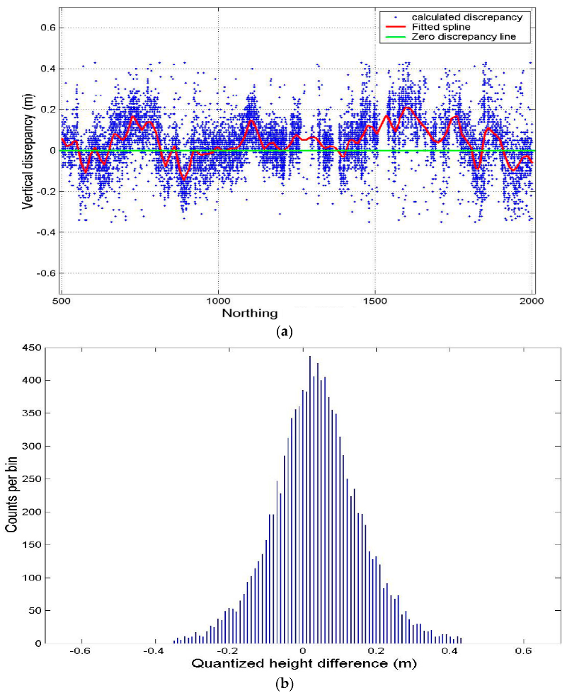
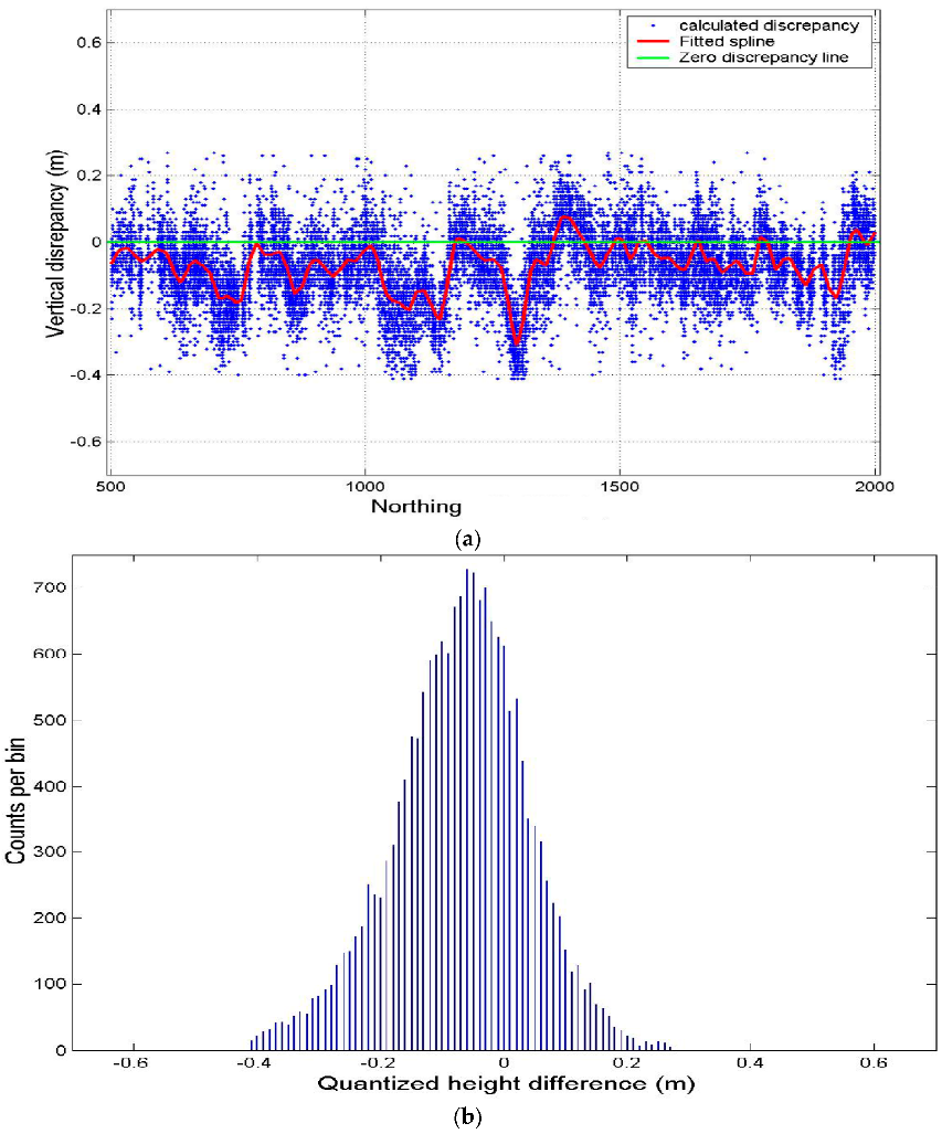
Figure 6a shows the discrepancy behavior with respect to time (North–South direction) and Figure 6b shows the histogram of the computed discrepancy for the overlap region between strips 1 and 2. In this overlap region, the average relative offset was 0.04m, which means the left data strip (strip 1) was higher in average than the right-hand strip (strip 2). On the other hand, Figure 7a,b show the relative height offset between strips 7 and 8 where the left strip (strip 7) seems to be below the right-hand one (strip 8) over most of the overlap region.
In general, the mean of the discrepancies does not equal zero and is not consistent with all strips. In addition, offsets are not purely a result of height differences at exactly corresponding points in the two strips since they are not error-free in planimetric positioning. Consequently, due to this planimetric uncertainty, the compared points might not have the same exact planimetric position and this mis-correspondence may contribute to the height differences. This correlation between height and planimetric offsets is to be expected in sloping surfaces.
4. Data Absolute Accuracy
Many sources of error affect the quality of airborne laser scanning data. Companies that work in collecting such datasets usually publish a fixed number for the uncertainty of their data. However, these numbers are usually not verified by the users because this is not a simple task. Correspondence between laser data points and ground points is not a straightforward matter. The absolute displacements can be found by measuring the location on the ground of a point or feature of known coordinates in the data set and comparing the two measurements.
4.1. Absolute Height Accuracy
The ground points were collected in a specific pattern except when on distinct features (ditches and curves on the ground). This pattern (lines) facilitates establishing a correspondence between the two data types. A buffer zone (with a width of one meter) was constructed around each ground data line and the data points inside that buffer zone were identified. Then, for each laser data point that lies within a meter or less from two ground data points, a corresponding height point with the same planimetric position was interpolated from the surrounding ground-surveyed points. The absolute accuracy was then estimated as the absolute difference between the laser height and the ground height. Since the points are nearby and the surface is flat, a linear interpolation was used. In order to minimize the effect of the planimetric uncertainty of the laser data, the interpolation was limited to totally flat areas. The slope of those areas was restricted to not exceed 10%. The slope was calculated as the rate of change of elevation for each LIDAR point using the Surface Slope tool in ArcMap.
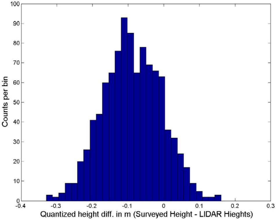
Direct differencing was applied to compute the discrepancy between the two data points from the laser and ground, i.e., the laser height was subtracted from the ground interpolated height. More than a thousand such differences were computed. Figure 8 shows the histogram of those differences. The histogram shows a bias in the differences of −0.088 m with a standard deviation of ±0.082 m. Hence, the average height of the laser data points included in the test is higher than the estimated ground by 0.088 m. Consequently, the total RMSE of the LIDAR heights from the surveyed ground (zero in the histogram) was 0.12 m with a mean value of zero. The calculated statistical characteristics represent only a small sample of the data. The tested area covers less than 2 s of collection time (about 19,000 data points since the designed scanning rate is 10,000 points/s). The 19,000 data points represent a small portion of the whole data set which is more than 3,000,000 data points. However, only 1008 points were included in the real computation since it is not practical to survey more points on the ground.
4.2. Absolute Planimetric Accuracy
Planimetric offsets are more complicated to determine since they require identifiable spatial features to establish the correspondence between the two data sets. Such features and locations for estimating the offsets might not be available, or when they exist, are usually limited. Moreover, identifying these locations is costly in time and requires great care in order to be reliable. Drainage ditches, terrain features, and building gable roofs are some examples of such features. Procedures and results of estimating the planimetric accuracy in both directions (Easting and Northing) are presented in this section.
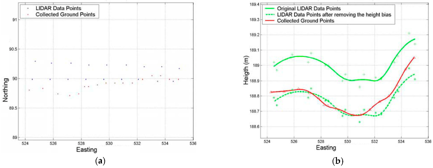
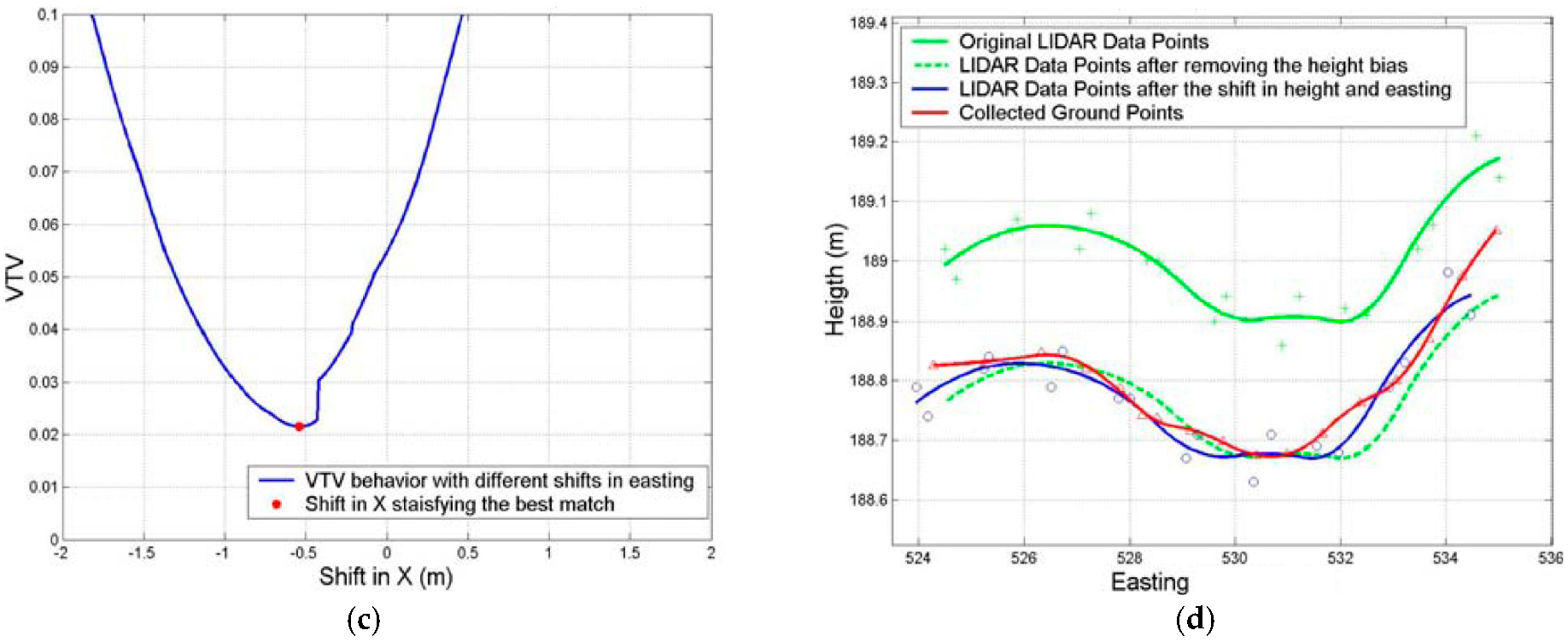
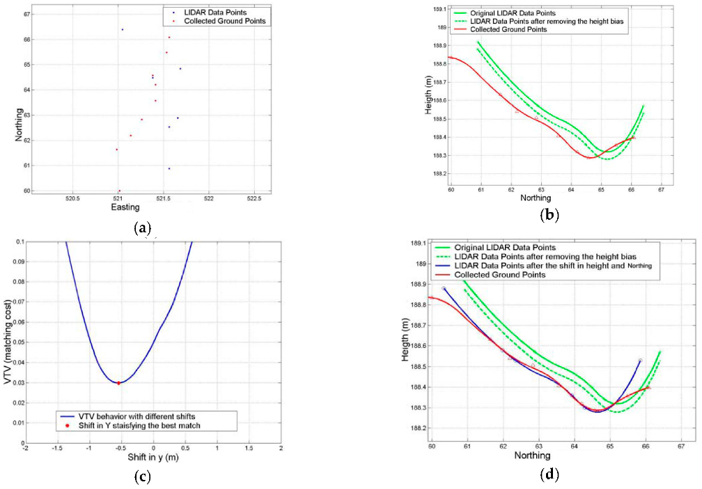
Eight positions were identified and used in obtaining the planimetric accuracy. Six of those locations were used to compute the offset in the X (Easting) direction and the other two were utilized to compute the offset in the Y (Northing) direction. In each of these locations the data points from both data sets, LIDAR and ground, were identified as shown in part (a) of Figure 9, Figure 10 and Figure 11. Parts (a) of these figures show the plan view of the points. From each set, an estimate of the two shifts was made to realize the coincidence. The idea here is to translate these two curves and obtain the shift that will maximize the match. Prior to that, the height bias should be removed in order to exclude its effect in the matching. In part (b) of the figures, the green dashed curve represents the LIDAR data after removing the height bias between the two data curves.
To get the best match between the two curves, the LIDAR data curve will be shifted gradually around the ground data set in the direction of the computed offset (X as in Figure 9 and Figure 10, and Y as in Figure 11). The shift search window ranged from −2 m to 2 m with an increment of 0.01m. At each increment, the discrepancy in Z of each ground point and its interpolated-correspondence point from the LIDAR curve data is computed. The sum of the squares of these offsets is considered as the matching cost at each location. Parts (c) of the figures show the matching cost function behavior with respect to different shift values. At the minimum matching cost, which is associated with the best match between the two curves, the corresponding shift is obtained. Parts (d) show the original data curves, after removing the height bias, and after the planimetric shift.
As stated above, eight locations were tested to obtain the planimetric shift. Table 2 summarizes the results at those selected locations. Regarding the offset in the X (Easting) direction, which is across the flight direction and coincides with the scanning direction, six locations were selected, three at the edge of the swath width of strip two and the rest at the middle of the strip. As expected at the strip edge, the offset in the scanning direction (−0.60 m as an average) was larger than at the middle of the strip (−0.30 m as an average). However, those shifts were in the same direction. The same thing could be said for the height bias, height offsets seem to be larger in magnitude at the edge of the strip. On the other hand, two locations were selected to test the accuracy along the flight direction Y (Northing), one at the middle of the strip and the other at the edge. The two locations had the same direction.
4.3. Error Behavior with Respect to Time
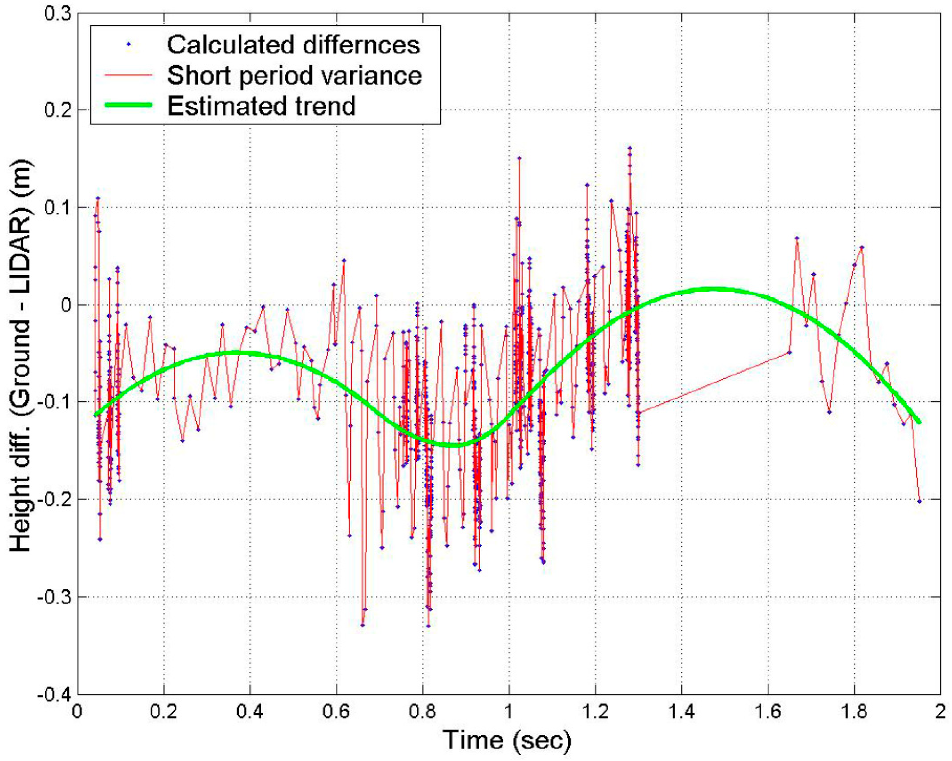
To show how errors changed while the scanner was advancing, the LIDAR data points over the test area were sorted based on the time they were scanned. Then, the calculated height differences (1008 biases) were sorted by time. The test area covered only less than two seconds of the scanning time, which contains about 19,000 data points. Figure 12 shows the behavior of the absolute height error with respect to the time they were scanned.
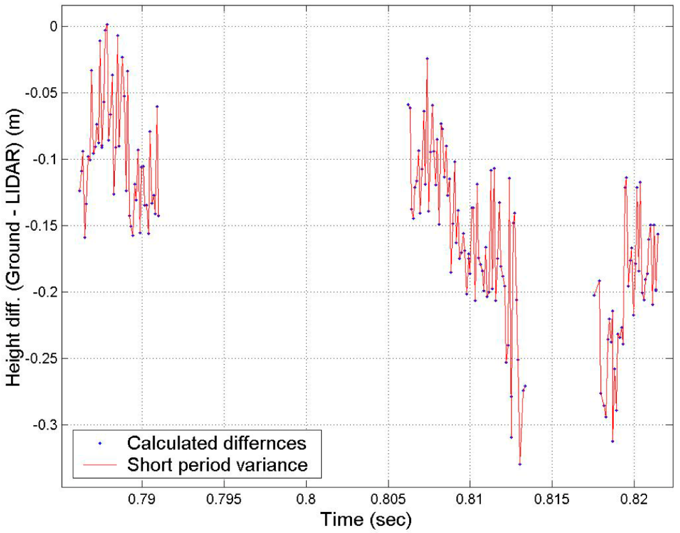
In Figure 12, the height differences between the LIDAR points and their corresponding ground-surveyed points show two types of variations. The two types can be divided in two components: a bias in the geo positioning system and a random variation around that bias. The first type of variation is called short-period variation. This variation seems to be random and has a high frequency. This variation between two consecutive points could reach 0.30 m as a maximum within 0.001 s. This random variation has a standard deviation of 0.082 m. The short period variation, Figure 13, of the uncertainty of LIDAR heights gives an indication of the system precision since the consecutive points are so close to each other in the time domain and the test was conducted on a flat surface where the height is approximately the same.
On the other hand, as shown in Figure 12, a trend (green spline) of the differences is observed which is the second form of the variation. A trend is defined as the component of a random phenomenon which has a period larger than the recorded data sample. The trend in this test data represents the biases in the geopositioning system. Although the test data represents only a small sample, this trend is very noticeable. The relative height accuracy between data strips confirms this inference regarding the two forms of random variation since the computation of the relative accuracy covers most of the data.
The total computed uncertainty of the LIDAR heights over the test area is about ±0.121 m. This uncertainty consists of two components: biases in the geopositioning of the platform and random variation around these biases due to the ranging system uncertainty. Regarding the planimetric accuracy, the computed offsets in the scanning direction over the test area show two main outcomes. First, the planimetric uncertainty is larger (almost double) at the end of the swath than at the middle. So, in general, the planimetric accuracy seems to vary based on the location along the scan (cross-track) direction. At the edge of the swath, the average offset was about 0.60 m, while at the middle it was about 0.30 m. The second outcome is that the whole strip seems to be shifted in the east direction since all the computed offsets have the same direction.
Both accuracies, relative and absolute, show two types of variation. The first variation form is the short period random variation which has a high frequency with time. This random variation seems to represent the actual precision of the LIDAR subsystem. The other variation form is the long period variation or a trend. This trend has a much lower frequency and seems to be a result of errors in the positioning/altitude subsystem. If this trend is modeled and the data is adjusted accordingly, the accuracy of data will be improved. Testing more samples that cover different parts with a longer period of time would be needed to strengthen these conclusions.
5. Results Analysis and Discussion
The relative height offsets between LIDAR data strips were examined based on the height offsets between coincident or partially coincident data points. More than 16,600 height offsets from all the 13 test overlap regions were computed. The results show a variation in the height offset between adjacent strips. Among the 13 overlap regions between adjacent strips, the average relative height offset ranges from 0 to 0.12 m. The maximum offset between coincident laser measurements from two different strips is about 0.40 m. Two variation types are observed in the discrepancy between adjacent strips, short- and long-period variations. The short-period variation is attributed with a high frequency with time and has a standard deviation of about ±0.10 m. The long-period variation has a much lower frequency than the first type. The source of the short-period variation appears to be the uncertainty in the LIDAR subsystem. Ranging and scanning observation uncertainty are some examples of error sources in the LIDAR subsystem. The short-period variation appears to be random and represents the LIDAR subsystem precision. On the other hand, the uncertainty in the navigation subsystem appears to be the source of the long-period variation, which can be modeled and corrected and consequently improve the data quality.
More than 1000 height discrepancies between the LIDAR data and collected ground points were calculated in order to examine the height absolute accuracy of the LIDAR data. The histogram of the computed differences shows a bias of about 0.088 m from the surveyed ground with a standard deviation of ±0.082 m around the middle of the histogram. The average height of the laser data points included in the test is higher than the estimated ground by 0.088 m. However, the total variation of the LIDAR heights from the surveyed ground is 0.120 m. This variation contains both the biases and its random differences. This number (0.120 m) represents a sample of the real system height precision of the LIDAR data. The computed discrepancies were then sorted based on the time they were scanned in order to examine the error behavior with respect to time. The height differences between the LIDAR points and their corresponding ground-surveyed points showed the two types of variation that were shown in the relative height accuracy. However, this time the tested sample is much smaller than in the relative height accuracy.
The variation between two consecutive points in time could reach 0.30 m as a maximum. The time span between two consecutive points in the test data is about 0.001 s since the pulse rate is 10 kHz. This short-period variation of the uncertainty of LIDAR heights gives an indication of the system precision since the consecutive points are so close to each other in the time domain and the test was conducted on a generally flat surface where the height is approximately the same.
In the scanning direction (across track), the planimetric offset of the LIDAR data from the collected ground points varies based on the location in the swath. As expected, at the strip edge, the offset in the scanning direction (−0.60 m as an average) was larger than at the middle of the strip (−0.30 m as an average). However, those shifts were in the same direction, which show the presence of a trend or bias. In the other direction (along track), the average offset from the ground was about 0.47 m. In general, the root mean square error of the planimetric offsets in both directions was estimated to be 0.50 m.
6. Conclusions
Coincident LIDAR data points in overlap regions between adjacent strips show a relative discrepancy in height. This discrepancy varies from one position to another and varies with time. Regarding the absolute height accuracy, the data points show a systematic departure from the collected ground reference and a random variation of −0.088 m. The total computed RMSE of the test data from the ground reference was about 12 cm. Planimetric offset of the LIDAR data from the ground reference in the across flight direction varies with the location in the swath. At the edge of the swath, the average planimetric offset was almost double its value in the middle.
Both relative and absolute height discrepancies of the LIDAR data have two components of variation. The first component is the short-period variation, which is random and has high frequency with time. This short-period random variation runs over the second component, which is the long-period variation. The long-period variation has a much lower frequency than the first type and represents the biases in the geopositioning system. The short-period variation is attributed to the LIDAR subsystem measurement uncertainty. System ranging resolution and scanning system-pointing precision are some examples of the error sources in the LIDAR subsystem. On the other hand, the uncertainty in the navigation subsystem appears to be the source of the long period variation, which can be modeled and accounted for in order to improve the quality of the data.
The LIDAR data accuracy evaluation is still an open area for more research and analysis, particularly with the growing application of new UAV-LIDAR systems in many applications. Such systems can provide centimeter-level accuracy and the procedure outlined in this research has the capability to evaluate the accuracy of these systems with a high degree of certainty. This will extend the use of LIDAR data in many applications such as building information models (BIMs), 3D Geographic Information Systems (GIS), mobile communications, disaster management, and city planning. Therefore, future research will focus on assessing the quality of LIDAR data produced from UAV systems and best practices of collecting LIDAR data for different applications.
Author Contributions
Methodology, A.A.; Validation, A.A.; Formal analysis, A.E.; Investigation, T.A. and A.A.; Resources, T.A.; Data curation, A.E.; Writing—original draft, A.E.; Writing—review & editing, T.A.; Project administration, A.E.; Funding acquisition, A.A. All authors have read and agreed to the published version of the manuscript.
Funding
This research received no external funding.
Data Availability Statement
Not applicable.
Conflicts of Interest
The authors declare no conflict of interest.
References
- Wani, Z.M.; Nagai, M. An approach for the precise DEM generation in urban environments using multi-GNSS. Measurement 2021, 177, 109311. [Google Scholar] [CrossRef]
- Gargoum, S.A.; El Basyouny, K. A literature synthesis of LiDAR applications in transportation: Feature extraction and geometric assessments of highways. GISci. Remote Sens. 2019, 56, 864–893. [Google Scholar] [CrossRef]
- Kulawiak, M. A Cost-Effective Method for Reconstructing City-Building 3D Models from Sparse Lidar Point Clouds. Remote Sens. 2022, 14, 1278. [Google Scholar] [CrossRef]
- Lv, D.; Ying, X.; Cui, Y.; Song, J.; Qian, K.; Li, M. Research on the technology of LIDAR data processing. In Proceedings of the First International Conference on Electronics Instrumentation and Information Systems (EIIS), Harbin, China, 3–5 June 2017. [Google Scholar]
- Elaksher, A.F. Co-registering satellite images and LIDAR DEMs through straight lines. Int. J. Image Data Fusion 2016, 7, 103–118. [Google Scholar] [CrossRef]
- Li, X.; Liu, C.; Wang, Z.; Xie, X.; Li, D.; Xu, L. Airborne LiDAR: State-of-the-art of system design, technology and application. Meas. Sci. Technol. 2020, 32, 032002. [Google Scholar] [CrossRef]
- Wehr, A. LiDAR systems and calibration. In Topographic Laser Ranging and Scanning, 2nd ed.; Shan, J., Toth, C., Eds.; CRC Press: Boca Raton, FL, USA, 2018; pp. 159–200. [Google Scholar]
- Elaksher, A.; Bhandari, S.; Carreon-Limones, C.; Lauf, R. Potential of UAV lidar systems for geospatial mapping. In Proceedings of the SPIE Optical Engineering and Applications, San Diego, CA, USA, 6–10 August 2017. [Google Scholar]
- Cao, S.; Weng, Q.; Du, M.; Li, B.; Zhong, R.; Mo, Y. Multi-scale three-dimensional detection of urban buildings using aerial LiDAR data. GISci. Remote Sens. 2020, 57, 1125–1143. [Google Scholar] [CrossRef]
- Megahed, Y.; Shaker, A.; Yan, W. Fusion of airborne LiDAR point clouds and aerial images for heterogeneous land-use urban mapping. Remote Sens. 2021, 13, 814. [Google Scholar] [CrossRef]
- Wang, X.; Li, P. Extraction of urban building damage using spectral, height and corner information from VHR satellite images and airborne LiDAR data. ISPRS J. Photogramm. Remote Sens. 2020, 159, 322–336. [Google Scholar] [CrossRef]
- Muhadi, N.A.; Abdullah, A.F.; Bejo, S.K.; Mahadi, M.R.; Mijic, A. The use of LiDAR-derived DEM in flood applications: A review. Remote Sens. 2021, 12, 2308. [Google Scholar] [CrossRef]
- Görüm, T. Landslide recognition and mapping in a mixed forest environment from airborne LiDAR data. Eng. Geol. 2019, 258, 105155. [Google Scholar] [CrossRef]
- Štular, B.; Lozić, E.; Eichert, S. Airborne LiDAR-derived digital elevation model for archaeology. Remote Sens. 2021, 13, 1855. [Google Scholar] [CrossRef]
- Mesa-Mingorance, J.L.; Ariza-López, F.J. Accuracy assessment of digital elevation models (DEMs): A critical review of practices of the past three decades. Remote Sens. 2021, 12, 2630. [Google Scholar] [CrossRef]
- Szypuła, B. Quality assessment of DEM derived from topographic maps for geomorphometric purposes. Open Geosci. 2019, 11, 843–865. [Google Scholar] [CrossRef]
- Montealegre, A.L.; Lamelas, M.T.; Riva, J.D. Interpolation routines assessment in ALS-derived digital elevation models for forestry applications. Remote Sens. 2015, 7, 8631–8654. [Google Scholar] [CrossRef] [Green Version]
- Gillin, C.P.; Bailey, S.W.; McGuire, K.J.; Prisley, S.P. Evaluation of LiDAR-derived DEMs through terrain analysis and field comparison. Photogramm. Eng. Remote Sens. 2015, 81, 387–396. [Google Scholar] [CrossRef] [Green Version]
- Von Schwerin, J.; Richards-Rissetto, H.; Remondino, F.; Spera, M.; Auer, M.; Billen, N.; Reindel, M. Airborne LiDAR acquisition, post-processing and accuracy-checking for a 3D WebGIS of Copan, Honduras. J. Archaeol. Sci. Rep. 2016, 5, 85–104. [Google Scholar] [CrossRef] [Green Version]
- Ali, T. On the selection of an interpolation method for creating a terrain model (TM) from LIDAR data. In Proceedings of the American Congress on Surveying and Mapping (ACSM) Conference, Nashville, TN, USA, 16–21 April 2004. [Google Scholar]
- Ali, T.; Mehrabian, A. A novel computational paradigm for creating a triangular irregular network (TIN) from LiDAR data. Nonlinear Anal. Theory Methods Appl. 2009, 71, e624–e629. [Google Scholar] [CrossRef]
- Ali, T. Building of robust multi-scale representations of LiDAR-based digital terrain model based on scale-space theory. Opt. Lasers Eng. 2010, 48, 316–319. [Google Scholar] [CrossRef]
- Contreras, M.; Staats, W.; Yiang, J.; Parrott, D. Quantifying the accuracy of LiDAR-derived DEM in deciduous eastern forests of the Cumberland Plateau. J. Geogr. Inf. Syst. 2017, 9, 339–353. [Google Scholar] [CrossRef] [Green Version]
- Sibona, E.; Vitali, A.; Meloni, F.; Caffo, L.; Dotta, A.; Lingua, E.; Garbarino, M. Direct measurement of tree height provides different results on the assessment of LiDAR accuracy. Forests 2016, 8, 7. [Google Scholar] [CrossRef]
- Guerra-Hernández, J.; Cosenza, D.N.; Rodriguez, L.C.E.; Silva, M.; Tomé, M.; Díaz-Varela, R.A.; González-Ferreiro, E. Comparison of ALS-and UAV (SfM)-derived high-density point clouds for individual tree detection in Eucalyptus plantations. Int. J. Remote Sens. 2018, 39, 5211–5235. [Google Scholar] [CrossRef]
- Schmelz, W.J.; Psuty, N.P. Quantification of Airborne Lidar Accuracy in Coastal Dunes (Fire Island, New York). Photogramm. Eng. Remote Sens. 2019, 85, 133–144. [Google Scholar] [CrossRef]
- Kovanič, Ľ.; Blistan, P.; Urban, R.; Štroner, M.; Blišťanová, M.; Bartoš, K.; Pukanská, K. Analysis of the Suitability of High-Resolution DEM Obtained Using ALS and UAS (SfM) for the Identification of Changes and Monitoring the Development of Selected Geohazards in the Alpine Environment—A Case Study in High Tatras, Slovakia. Remote Sens. 2020, 12, 3901. [Google Scholar] [CrossRef]
- Cățeanu, M.; Ciubotaru, A. Accuracy of Ground Surface Interpolation from Airborne Laser Scanning (ALS) Data in Dense Forest Cover. ISPRS Int. J. Geo-Inf. 2020, 9, 224. [Google Scholar] [CrossRef] [Green Version]
- Cățeanu, M.; Ciubotaru, A. The effect of lidar sampling density on DTM accuracy for areas with heavy forest cover. Forests 2021, 12, 265. [Google Scholar] [CrossRef]
- Liu, X. A new framework for accuracy assessment of LIDAR-derived digital elevation models. ISPRS Ann. Photogramm. Remote Sens. Spat. Inf. Sci. 2022, 4, 67–73. [Google Scholar] [CrossRef]
- Ussyshkin, R.V.; Smith, B. Performance analysis of ALTM 3100EA: Instrument specifications and accuracy of lidar data. In Proceedings of the ISPRS Commission I Symposium, Paris, France, 4–6 July 2006. [Google Scholar]
- Mostafa, M.; Hutton, J.; Reid, B.; Hill, R. GPS/IMU products—The Applanix approach. In Photogrammetric Week; Wichmann: Berlin/Heidelberg, Germany, 2001; Volume 1, pp. 63–83. [Google Scholar]
- Vosselman, G.; Maas, H.G. Adjustment and filtering of raw laser altimetry data. In Proceedings of the OEEPE Workshop on Airborne Laser Scanning and Interferometric SAR for Detailed Digital Terrain Models, Stockholm, Sweden, 1–3 March 2001. [Google Scholar]
Figure 1.
Area coverage of a portion of the 14 strips.
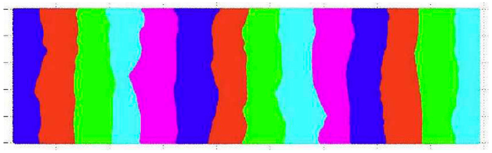
Figure 2.
The athletic area where the topographical survey was conducted.
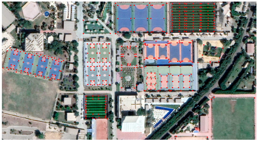
Figure 3.
Profile of the overlap area (2 m width) between (a) strip 1 and 2, (b) strip 2 and 3.

Figure 4.
Closer View of the Overlap Region.
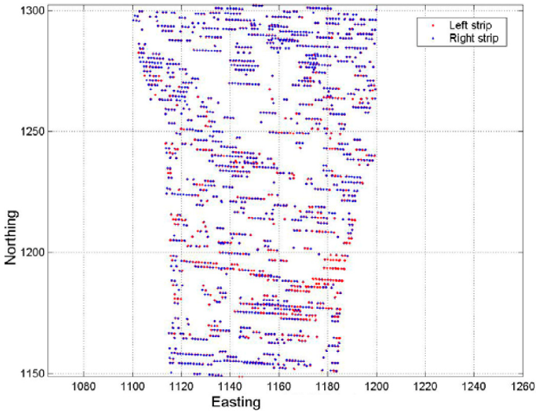
Figure 5.
Mean Relative discrepancy behavior between adjacent strips, where the x-axis represents the overlap regions (where 1 is the overlap region between strip one and two).
Figure 5.
Mean Relative discrepancy behavior between adjacent strips, where the x-axis represents the overlap regions (where 1 is the overlap region between strip one and two).
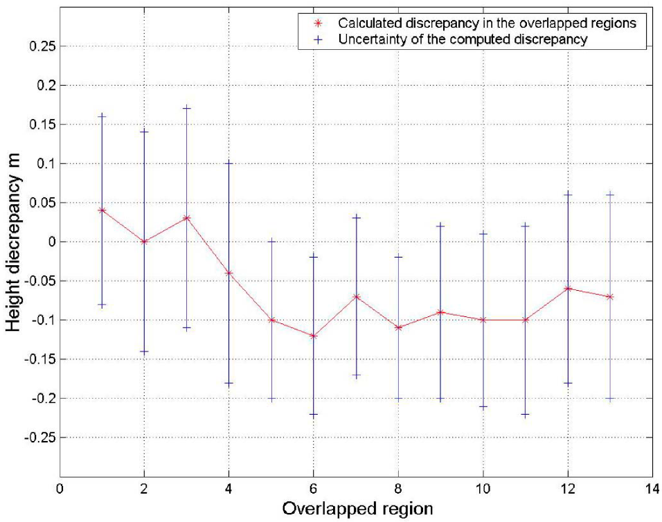
Figure 6.
(a): Relative height discrepancy along the North–South direction in the overlap region between the 1st and the 2nd strip. (b): The histogram of relative height discrepancy between the 1st strip and the 2nd strip.
Figure 6.
(a): Relative height discrepancy along the North–South direction in the overlap region between the 1st and the 2nd strip. (b): The histogram of relative height discrepancy between the 1st strip and the 2nd strip.

Figure 7.
(a): Relative height discrepancy along the North–South direction in the overlap region between the 7th and the 8th strip. (b): The histogram of the relative height discrepancy between the 7th strip and the 8th strip.
Figure 7.
(a): Relative height discrepancy along the North–South direction in the overlap region between the 7th and the 8th strip. (b): The histogram of the relative height discrepancy between the 7th strip and the 8th strip.

Figure 8.
Height differences histogram between the laser height and the ground height.

Figure 9.
(a–d) Planimetric offset in Easting (X) direction at location A.


Figure 10.
(a–d) Planimetric offset in Easting (X) direction at location B.
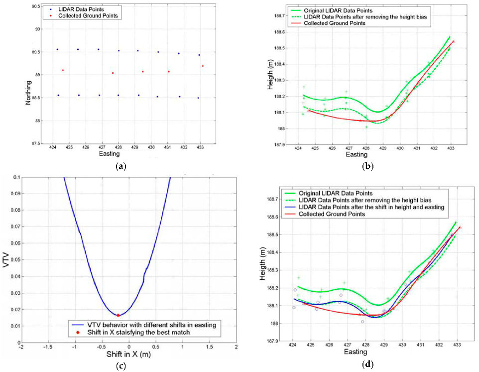
Figure 11.
(a–d) Planimetric offset in Northing (Y) direction at location G.

Figure 12.
Height accuracy (Ground—LIDAR) with respect to time.

Figure 13.
Short period variation of the height biases.


Table 1.
Relative height discrepancy between adjacent data strips.
| 1,2 | 2,3 | 3,4 | 4,5 | 5,6 | 6,7 | 7,8 | 8.9 | 9,10 | 10,11 | 11,12 | 12,13 | 13,14 | ||
|---|---|---|---|---|---|---|---|---|---|---|---|---|---|---|
| 0.05 m | #pts | 521 | 474 | 587 | 552 | 658 | 576 | 0.10 | 539 | 725 | 626 | 649 | 517 | 492 |
| Mean ΔH(m) | 0.04 | 0.00 | 0.03 | −0.04 | −0.10 | −0.12 | −0.07 | −0.11 | −0.09 | −0.10 | −0.10 | −0.06 | −0.07 | |
| STD m | 0.12 | 0.14 | 0.14 | 0.14 | 0.10 | 0.10 | 0.10 | 0.09 | 0.11 | 0.11 | 0.12 | 0.12 | 0.13 | |
| 0.10 m | #pts | 2017 | 2019 | 2193 | 2108 | 2667 | 2304 | 3172 | 2087 | 2880 | 2583 | 2616 | 2085 | 2121 |
| Mean ΔH m | 0.04 | 0.00 | 0.03 | −0.04 | −0.10 | −0.11 | −0.07 | −0.11 | −0.09 | −0.09 | −0.10 | −0.06 | −0.07 | |
| STD m | 0.12 | 0.15 | 0.14 | 0.14 | 0.11 | 0.10 | 0.10 | 0.10 | 0.11 | 0.11 | 0.11 | 0.11 | 0.12 | |
| 0.25 m | #pts | 10,891 | 11,017 | 11,944 | 11,872 | 14,761 | 11,889 | 17,702 | 11,014 | 14,768 | 13,986 | 13,951 | 11,242 | 11,142 |
| Mean ΔH m | 0.04 | 0.00 | 0.03 | −0.03 | −0.10 | −0.10 | −0.07 | −0.10 | −0.08 | −0.09 | −0.10 | −0.07 | −0.06 | |
| STD m | 0.12 | 0.15 | 0.14 | 0.15 | 0.11 | 0.11 | 0.11 | 0.11 | 0.11 | 0.12 | 0.12 | 0.12 | 0.10 |
Table 2.
Planimetric accuracy results.
| Location | Height Bias (m) | Direction | Plan. Offset | Location Description |
|---|---|---|---|---|
| A | −0.12 | X | −0.67 | At the right edge of the swath width of strip 2 |
| B | −0.03 | X | −0.29 | At the middle of the swath width of strip 2 |
| C | −0.23 | X | −0.54 | At the right edge of the swath width of strip 2 |
| D | −0.07 | X | −0.20 | At the middle of the swath width of strip 2 |
| E | −0.23 | X | −0.62 | At the right edge of the swath width of strip 2 |
| F | −0.08 | X | −0.43 | At the middle of the swath width of strip 2 |
| G | −0.04 | Y | −0.55 | At the middle of the swath width of strip 2 |
| H | −0.07 | Y | −0.40 | At the middle of the swath width of strip 2 |
Disclaimer/Publisher’s Note: The statements, opinions and data contained in all publications are solely those of the individual author(s) and contributor(s) and not of MDPI and/or the editor(s). MDPI and/or the editor(s) disclaim responsibility for any injury to people or property resulting from any ideas, methods, instructions or products referred to in the content. |
© 2023 by the authors. Licensee MDPI, Basel, Switzerland. This article is an open access article distributed under the terms and conditions of the Creative Commons Attribution (CC BY) license (https://creativecommons.org/licenses/by/4.0/).
Share and Cite
MDPI and ACS Style
Elaksher, A.; Ali, T.; Alharthy, A. A Quantitative Assessment of LIDAR Data Accuracy. Remote Sens. 2023, 15, 442. https://doi.org/10.3390/rs15020442
AMA Style
Elaksher A, Ali T, Alharthy A. A Quantitative Assessment of LIDAR Data Accuracy. Remote Sensing. 2023; 15(2):442. https://doi.org/10.3390/rs15020442
Chicago/Turabian StyleElaksher, Ahmed, Tarig Ali, and Abdullatif Alharthy. 2023. "A Quantitative Assessment of LIDAR Data Accuracy" Remote Sensing 15, no. 2: 442. https://doi.org/10.3390/rs15020442
Note that from the first issue of 2016, this journal uses article numbers instead of page numbers. See further details here.