A Three Stage Optimal Scheduling Algorithm for AGV Route Planning Considering Collision Avoidance under Speed Control Strategy

Abstract

With the trend of terminal automation and the requirement for port operation efficiency to be greatly improved, it is very necessary to optimize the traveling route of automatic guided vehicles (AGV) with reference to the connection of loading and unloading equipment. As a complex multi-equipment system, it is inevitable that AGV will collide when traveling due to various accidents in actual operation, which will lead to AGV locking and reduce the efficiency of terminal operation. Considering the locking problem of AGV, we propose a three-stage integrated scheduling algorithm for AGV route planning. Through joint optimization with quay cranes (QC) and yard blocks, a road network model is established in the front area of the container port to optimize the path of AGV in the road network, and a speed control strategy is proposed to solve the problem of AGV collision avoidance. In the first stage, we establish the AGV optimal route model with the goal of minimizing the AGV path according to the AGV road network situation. In the second stage, on the basis of the determination of AGV route planning, and when the container task is known, the AGV task assignment model is established with the goal of minimizing the maximum completion time, and the model is solved by genetic algorithm (GA). In the third stage, on the basis of AGV task assignment and route determination, the AGV route and AGV task assignment scheme are input into the simulation model by establishing the AGV collision avoidance control model for speed control, and establishing the AGV route network simulation model for automated terminals considering collision avoidance in plant simulation software. The maximum completion time obtained from the simulation model is compared with the completion time obtained from the genetic algorithm. The proposed three-stage joint scheduling algorithm can improve the loading and unloading efficiency of the port, reduce the AGV locking situation, and has a certain contribution to the formulation of the actual operation planning of the port.

1. Introduction

With the increasing number of shipping containers and the rising cost of port manual operations [1], intelligence, unmanned, and automation are becoming the trends of port development. As the most representative equipment of an unmanned port, AGV are the main carriers of horizontal transportation at the front of the automated terminal. AGV can carry out container transportation along the specified automatic guidance route according to the operation instructions. Due to the advantages of convenient operation, intelligence, and integration, AGV are safer, more efficient, and more environmentally friendly than traditional container truck transportation. With the development of automated terminals and the application of AGV, their advantages are revealed, while their problems are gradually exposed. The operation environment of automated terminals is relatively complex, which manifests in dynamic, random, sudden, and other uncertainties, making the AGV path planning problem more complex. At the same time, AGV are an important link connecting the shore and the yard, which greatly impact the operation efficiency and overall operation of the entire terminal. As container ports are a complex multi-system aggregation [2,3], once the AGV break down or collide with other AGV on the original routing, it will cause the AGV to lock up, aggravating the traffic congestion of the terminal, which is not conducive to the improvement of port traffic efficiency and the reduction of operating costs. Therefore, current research focuses on the efficient container transport route planning of AGV in the terminal. An increasing number of experts and scholars have conducted research on AGV scheduling, AGV routes, and AGV collision avoidance. Qiu et al. [4] introduced the problem of AGV scheduling and routing, investigated and classified the main existing algorithms, and pointed out that the existing algorithms are only suitable for small-scale use of AGV. AGV scheduling optimization is to allocate tasks and path planning for AGV according to container operation tasks [5]. The purpose of scheduling optimization includes one or more of the following: shortest formal path, shortest total operation time, and lowest operating cost. Kim et al. [6] used an integer programming model to study the AGV scheduling problem of automated terminals with the objective of minimizing the total delay time of tasks and the total transportation cost of AGV. Xin et al. [7] put forward an equipment rescheduling method based on the current state to reduce the impact of interference (such as job delay or machine failure) on operation efficiency, aiming at the problem that the current container terminal scheduling is mostly offline scheduling, which reduces the container handling delay time and saves energy consumption. Confessore et al. [8] established a model for the AGV scheduling problem, gave a mixed integer programming model with the shortest running time as the goal, and solved the running route and task order of AGV by using a soft time window and penalty factor constraints. Errico et al. [9] established the hard time window and random processing time model of the AGV route based on the branching method and cutting plane rule. Wu et al. [10] developed a novel AGV multi-state scheduling algorithm (MSSA), which achieved a good trade-off between AGV utilization and total processing span. Compared with the traditional idle scheduling strategy, MSSA schedules more AGV and tasks in each calculation, making its optimization goal closer to the global optimization goal. Li et al. [11] studied the relationship between AGV scheduling tasks, charging threshold, and power consumption in the smart factory, and jointly optimizing the AGV charging problem and the AGV operation sequence.

AGV route planning is mainly divided into two categories: one is static research, and the other is dynamic research [12]. In the research of static path planning, Zhong et al. [13] proposed a mixed integer planning model based on path optimization, integrated scheduling, conflicts, and deadlocks to minimize the delay time of AGV under the condition of known task allocation, and conducted large-scale and small-scale experiments to prove the effectiveness of the model. Chen et al. [14] developed an effective routing of multiple AGV based on the repulsive potential field optimized ant agent (Rf Ant agent). Aiming at the congestion phenomenon of nodes, they introduced a guiding factor into the path node selection model to determine the direction of AGV in the centralized control node. Xing et al. [15] proposed a novel tabu search (NTS) algorithm to solve the conflict when multiple AGV work at the same time in the automatic warehouse, which improved the efficiency of AGV picking goods in the automatic warehouse. According to the location of each picking point in the warehouse, and the initial solution generation and termination conditions in the proposed algorithm, relocation and exchange operations were designed for the neighborhood search process. Homayouni et al. [16,17] studied the basic scheduling problem of AGVs and QCs. Taking the maximum completion time of QCs as the object, a mixed integer programming model was proposed by combining a quadratic genetic algorithm (GA) with a simulated annealing method. As for the research on static route planning, scholars mainly model and solve AGV route planning based on the stability of the static road network, with the goal of minimizing the total travel distance, and rarely consider AGV scheduling and AGV collision avoidance.

In the process of automated terminal AGV transporting of containers, due to the unmanned operation state, the implementation of AGV operation tasks will inevitably lead to hidden dangers of collision and deadlock. Jerzy et al. [18] divided the transport road network into nonoverlapping unidirectional regions, and the transmission network can be expressed as a segment composed of unidirectional regions and a segment composed of other regions. The effectiveness of the proposed method was verified by simulation. If they cannot be resolved, they will directly affect the implementation of AGV tasks. AGV cannot complete the scheduled tasks on time. Therefore, in the process of AGV transportation, it is also necessary to consider AGV conflict control during driving. Liu et al. [19] used Dijkstra algorithm to improve the optimal path search method of a single AGV. Priority based traffic rules were introduced into the directed graph, and the speed and geometric trajectory of the AGV were adjusted, thus effectively solving the collision and conflict between vehicles. Umar et al. [20] proposed a genetic algorithm using task priority to detect and avoid AGV conflicts in order to solve the path interference problem of AGV. Dimitri et al. [21] proposed a strategy based on time logic according to the problem of AGV collision avoidance in FMS, used time Petri nets to model, and proved its feasibility through simulation.

To sum up, the current literature on AGV route planning mainly focuses on the task allocation, route planning and collision avoidance of AGV. Most of the AGV route planning research on collision avoidance is based on intelligent factory. As a large logistics handling system, the automated terminal requires multiple operation subsystems to be optimized at the same time, so it has a certain complexity and challenge. The research on collision avoidance of AGV is generally based on the existing route to schedule the AGV in the collision. It ignores the impact of AGV’s task allocation on the route selection, so we propose a three-stage algorithm that combines heuristics and simulation, and uses the topology method to build an automatic container terminal network diagram. The AGV task allocation, route planning, and AGV collision avoidance are jointly optimized within a framework to reduce the AGV collision through a speed control strategy and improve the port operation efficiency

The remainder of this paper is organized as follows. Section 2 describes the problem formulation. Section 3 formulates three submodels about AGV route scheduling, AGV tasks assignment, and AGV collision avoidance control. Section 4 illustrates the framework of the proposed algorithm, the coding process, and the process of the simulation model. Case studies are presented in Section 5, and the conclusions are drawn in Section 6.

2. Problem Formulation

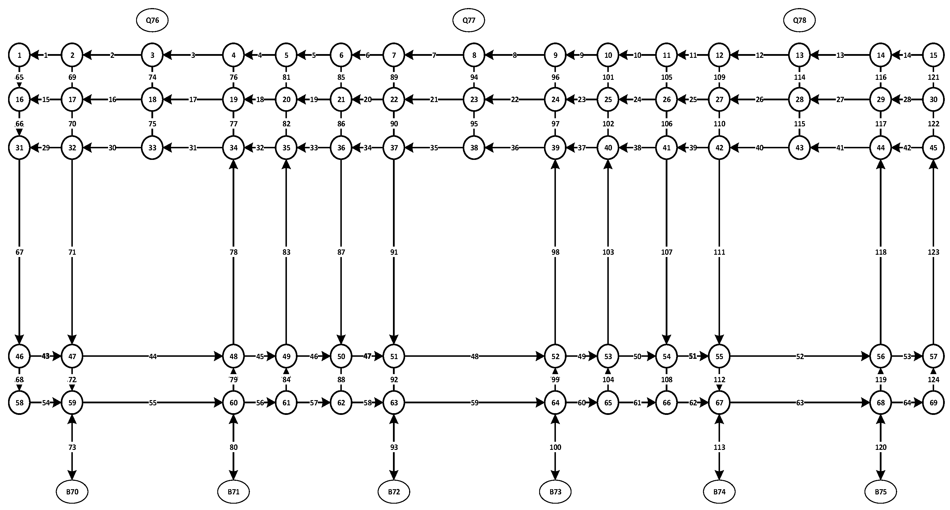
In the automatic terminal loading and unloading process, when a container ship is berthed and QC are loading and unloading the ship according to the port operation schedule, AGV are required to work cooperatively to unload the container from the QC and send it to the yard blocks. With the layout of an automated terminal as a reference, we built an AGV road network model, as shown in Figure 1. We can see that AGV travel in a given direction in the specified road network model. When receiving task information, they pick up containers at the designated block or QC and send them to the designated block or QC.

In the process of traveling, AGV have four handling and transportation modes: (1) only unloading, (2) only loading, (3) loading first and unloading later, and (4) unloading first and loading later. Due to the large number of container terminal operations, AGV may encounter collisions during travelling, which are mainly divided into three categories: (A) pursuit in the same direction, (B) conflict at interaction points, and (C) conflict in the opposite direction. With the layout of an automated terminal as a reference, we built an AGV road network model, as shown in Figure 1.

We can see that AGV travel in a given direction in the specified road network model. When receiving task information, they picks up boxes at the designated box area or quayside bridge and send them to the designated box area or quayside bridge. In the process of driving, AGV have four transportation modes: (1) unloading only, (2) loading only, (3) loading first and unloading later, and (4) unloading first and loading later. Due to the large volume of container terminal operations, AGV may encounter collisions during driving, which are mainly divided into three categories: (A) chasing conflict in the same direction, (B) interaction conflict, and (C) conflict in the opposite direction. In actual operation, AGV locking is a difficult problem. When planning AGV road strength, we should consider the environment and task allocation of the actual port operation area, and pay attention to collision avoidance.

The essence of AGV scheduling planning is the AGV route optimization problem. Therefore, the core work of this paper is to realize a collision avoidance design of AGV by optimizing the trajectory of AGV. At present, route planning of AGV is an important part of intelligent control systems and the key to ensure work safety. When encountering obstacles, the traditional path planning algorithm is mainly used to solve the problem when the robot encounters obstacles, to find and plan the correct path. There are two main types of AGV route planning: one is carried out in a static environment, and the other is carried out in a dynamic environment.

(1)

AGV route planning in the static environment

Under the condition of a static route network, AGV can sense the surrounding environment without fully understanding the surrounding environment, and use this method to determine the running trajectory of AGV. Therefore, this route is usually used when there are only static known obstacles in the environment. However, in order to plan the path of AGV in a stationary environment, the distance between the target point and the target must be determined first to avoid the existence of obstacles and blockage, and the shortest path needs to be planned to ensure that the AGV can reach the destination in the shortest time.

(2)

AGV route planning in the dynamic environment

Due to the changing environment, a lot of information cannot be controlled. Safety and timeliness should be taken into account when planning routes. No matter which performance metric you use, you need to consider target attraction, dynamic security, and time constraints. In a complex road network, due to the large number of AGV running, it is difficult for path planning to avoid path conflicts between vehicles, and at the same time, road deadlock caused by path conflicts cannot be eliminated, which will lead to traffic efficiency decline, and may lead to the standstill of the lateral traffic system.

Therefore, we propose a three-stage optimization algorithm for joint AGV route and task allocation, using GA to find the initial AGV route scheme. On this basis, in the simulation model, the proposed speed control strategy is to make adjustments to the route scheme to prevent collisions.

3. Modeling

This problem involves three mathematical models. Model 1 is the optimal route model of AGV. The objective is to minimize the traveling distance of AGV. The AGV transportation area network is the input data, and the output result is AGV route schedule. Figure 2 is the AGV transportation area network. Model 2 is the AGV task assignment model. The container task set is input data, and the output result is the assignment schedule of the container task. Model 3 is the AGV collision avoidance control model. The container assignment schedule and AGV route schedule are the input data, and the output result is the final driving scheme of AGV.

3.1. Assumptions

(1)

In order to simplify the modeling, the route of AGV is only unidirectional, so there will be no opposite conflict.

(2)

Only one AGV can be driving in any road section.

(3)

The actual loading and unloading time of a container by QC follows the normal distribution of (120, 20), when the standard operation time of loading and unloading each container by the QC is about 120 s.

(4)

Each task can only be completed by one AGV, and each AGV can only load one container at a time.

(5)

The berths and yard blocks served by an AGV are not fixed.

(6)

Ignore the weather, AGV damage, and other force majeure factors.

(7)

The number of AGV and QC is known.

(8)

The number of tasks and the corresponding loading and unloading blocks of each task are known.

3.2. AGV Route Modeling

Set
$Q$	Set of QCs’ nodes
$B$	Set of blocks’ nodes
$N$	Set of nods in the route network, $n\in N$.
$E$	Set of sections of the route between node a and node b, $e_{ab}\in E$.
$K$	Set of AGVs, $\mathrm{k}\in K$.
$J$	Set of containers, $J=J^{+}+J^{-}$
$J^{+}$	Set of loading containers
$J^{-}$	Set of unloading containers
$\overline{J}$	Set of all tasks, $\overline{J}=\{I+F\}+J$, $I$ is virtual started task, $F$ is virtual finished task
Parameter
$T_{qb}$	Set of traveling time between QC q and block b
${\mathrm{qt}}_{ij}$	The travelling time of AGVq transport task i and j
${\mathrm{t}}_{qj}$	The travelling time of AGVq transport task i
$s_{qij}$	The travelling time of AGVq transport task I and task j on empty state
$h_{qi}$	The waiting time of AGVq at QC i
$h_{bi}$	The waiting time of AGVq at block b
$g{p}_i$	The earliest time that the AGV can be operated at the QC for task i
$q{r}_j$	Time when quayside crane completes container task j, $q{r}_j=\{\begin{array}{l}q{p}_j,if \mathrm{h}=\mathrm{I}\\ q{r}_i+q{t}_{ij},else\end{array}$
$L$	The length of AGV
$L_s$	Safe distance to be kept by AGV when travelling or stopping for waiting
$v_0$	AGV’s normal constant speed
$v_1$	AGV deceleration speed
$a$	The acceleration of AGV acceleration and deceleration under speed control
$t_1$	The speed after AGV decelerates from normal speed
Decision variable:
$Z_{ij}$	1, if the route path from node i to node j; 0, otherwise.
${\mathrm{X}}_{abk}$	1, if AGV k chooses the route path from node a to node b; 0, otherwise.
$y_{ijk}$	1, AGV k completes task j after completing task i; 0, otherwise.

$$\min ({\displaystyle \sum _{i\in N}{X}_{qi}{e}_{qi}}+{\displaystyle \sum _{i.j\in N}{X}_{ij}{e}_{ij}}+{\displaystyle \sum _{j\in N}{X}_{jb}{e}_{jb}})$$

(1)

The objective function (1) is to minimize the total traveling distance of AGV from the QC to the yard block. AGV load (unload) containers at the QC and transport containers to the designated yard block through the AGV route network. The traveling distance of these three parts constitutes the total traveling distance from the QC to the yard block, and also corresponds to the first, second and third items in the formula.

$${\displaystyle \sum _{i\in N}{Z}_{qi}}={\displaystyle \sum _{j\in N}{Z}_{jb}},q\in Q,b\in B$$

(2)

$${\mathrm{Z}}_{ij}<X_{ijk},i,j\in N,\forall k\in \mathrm{K}$$

(3)

$${\displaystyle \sum _{i,j\in N}{X}_{ijk}}\le n-1,\forall k\in \mathrm{K}$$

(4)

Constraint (2) indicates that the AGV travelling path driving path is a cycle with a beginning and an end, and cannot be terminated halfway. Constraint (4) and (3) indicates the road section with node i to node j. Constraint (4) indicates elimination of sub-circuits.

3.3. AGV Task Assignment Modeling

Set
$J$	Set of containers, $J=J^{+}+J^{-}$
$J^{+}$	Set of loading containers
$J^{-}$	Set of unloading containers
$\overline{J}$	Set of all tasks, $\overline{J}=\{I+F\}+J$, $I$ is virtual started task, $F$ is virtual finished task
$T_{qb}$	Set of traveling time between QC q and block b
Parameter
${\mathrm{qt}}_{ij}$	The travelling time of AGVq transport task i and j
${\mathrm{t}}_{qj}$	The travelling time of AGVq transport task i
$s_{qij}$	The travelling time of AGVq transport task I and task j on empty state
$h_{qi}$	The waiting time of AGVq at QC i
$h_{bi}$	The waiting time of AGVq at block b
$g{p}_i$	The earliest time that the AGV can be operated at the QC for task i
$q{r}_j$	Time when quayside crane completes container task j, $q{r}_j=\{\begin{array}{l}q{p}_j,if \mathrm{h}=\mathrm{I}\\ q{r}_i+q{t}_{ij},else\end{array}$
$L$	The length of AGV
$L_s$	Safe distance to be kept by AGV when travelling or stopping for waiting
$v_0$	AGV’s normal constant speed
$v_1$	AGV deceleration speed
$v_2$	AGV acceleration speed
$a$	The acceleration of AGV acceleration and deceleration under speed control
$t_1$	The speed after AGV decelerates from normal speed
$L$	The length of AGV
$L_s$	Safe distance to be kept by AGV when travelling or stopping for waiting
$v_0$	AGV’s normal constant speed
$v_1$	AGV deceleration speed
Variable
$y_{ijk}$	1, AGV k completes task j after completing task i; 0, otherwise.

In the automated container terminal operation system in Figure 1, AGV have four transportation modes: (a) only unloading; (b) only loading; (c) loading first and unloading later; and (d) unloading first and loading later. Different transportation modes determine the empty travelling time and overall travelling time of AGV. For example, the empty car travelling time algorithm of the loading only mode and the loading first unloading mode is completely different, so it is necessary to classify $q{t}_{ij}$ and discuss $s_{ij}$, travelling time. $q{t}_{ij}$ represents the time interval between AGV arriving at the QC of task i and at the QC of task j. Because $q{t}_{ij}$ has different values under different loading and unloading task modes, the initial virtual start ends the task. $s_{ij}$ represents the deadhead time of the time interval between AGV arriving at the QC under task i and the QC under task j. $s_{ij}$ represents the time interval between AGV arriving at the QC of task i and the QC of task j. Under the above four transportation modes, the values of $q{t}_{ij}$ are:

The QC operation is carried out according to the QC operation priority sequence planning. The sequence of tasks should be considered when calculating $q{t}_{ij}$. For example, for the QC q, four loading and unloading tasks are arranged, and the third task is carried out after the first task completion. We explain the calculation of $q{t}_{ij}$, $s_{ij}$ under 4 different types in

Table 1. Time interval between AGV arriving at adjacent tasks.

	$j\in J^{+}$	$j\in J^{-}$
$i\in J^{+}$	$q{t}_{ij}=h_{qi}+s_{ij}+h_{bi}+t_j$	$q{t}_{ij}=h_{qi}+s_{ij}$
$i\in J^{-}$	$q{t}_{ij}=h_{qi}+t_i+h_{bi}+s_{ij}+h_{bj}+t_j$	$q{t}_{ij}=h_{qi}+t_i+h_{bi}+s_{ij}$

and

Table 2. Traveling time of AGV transport adjacent tasks on empty state.

	$j\in J^{+}$	$j\in J^{-}$
$i\in J^{+}$	$s_{ij}=t(q_i,b_j)$	$s_{ij}=t(q_i,b_j)$
$i\in J^{-}$	$s_{ij}=t(q_i,b_j)$	$s_{ij}=t(b_i,q_j)$

. M is a maximum number to ensure that the QC operate in the sequence of the operation priority sequence planning.

Under the four transportation modes, the meaning of deadhead time is different. Under the unloading mode, deadhead time is the time from the container area in the yard of the previous task to the quayside bridge position of the next task. The idling time in the packing mode is the time of moving from the quayside bridge position of the previous task to the container area of the storage yard of the next task. The deadhead time under the loading and unloading mode is the moving distance from the quayside bridge position of the previous task to the quayside bridge position of the next task, In the unloading before loading mode, the idling time is the moving distance from the container area in the storage yard of the previous task to the container area in the storage yard of the next task.

$h_{qi}$ is the AGV’s waiting time for container loading and unloading at the QC may occur in the following two situations due to the arrival of the QC:

(1)

AGV arrived late and the QC waited for AGV. $h_{qi}=(q{r}_j+q{t}_{ji})-q{p}_i$

(2)

AGV arrives early and needs to wait for the QC. $h_{qi}=q{p}_i-(q{r}_j+q{t}_{ji})$

$$\min \max {\displaystyle \sum _{j\in \overline{J}}{\displaystyle \sum _{i\in \overline{J}}q{t}_{ij}}}·y_{ijk}\hspace{1em}for \forall \mathrm{k}\in K$$

(5)

$${\displaystyle \sum _{\mathrm{k}\in K}{\displaystyle \sum _{j\in \overline{J}}{y}_{ijk}}}=1,for i\in J$$

(6)

$${\displaystyle \sum _{\mathrm{k}\in K}{\displaystyle \sum _{j\in \overline{J}}{y}_{ijk}}}=1,for j\in J$$

(7)

$${\displaystyle \sum _{i\in \overline{J}}{y}_{ihk}}-{\displaystyle \sum _{j\in \overline{J}}{y}_{hjk}}=0,for \forall h\in J,\forall k\in K$$

(8)

$${\displaystyle \sum _{j\in \overline{J}}{y}_{Ijk}}=1,for \forall k\in K$$

(9)

$${\displaystyle \sum _{i\in \overline{J}}{y}_{iFk}}=1,for \forall k\in K$$

(10)

$$y_{ijk}\in \{0,1\},for \forall i,j\in \overline{J},k\in K$$

(11)

$$q{t}_{ij}=(h_{qi}+t_i+h_{bi}+s_{ij})y_{ijk},i,j\in J^{-},k\in K$$

(12)

$$q{t}_{ij}=(h_{qi}+s_{ij}+h_{bi}+t_j)y_{ijk},i,j\in J^{+},k\in K$$

(13)

$$q{t}_{ij}=(h_{qi}+s_{ij})y_{ijk},i\in J^{+},j\in J^{-},k\in K$$

(14)

$$q{t}_{ij}=(h_{qi}+t_i+h_{bi}+s_{ij}+h_{bj}+t_j)y_{ijk},i\in J^{-},j\in J^{+},k\in K$$

(15)

$$s_{ij}=t(b_i,q_j)y_{ijk},i,j\in J^{-},k\in K$$

(16)

$$s_{ij}=t(q_i,b_j)y_{ijk},i,j\in J^{+},k\in K$$

(17)

$$s_{ij}=t(q_i,b_j)y_{ijk},i\in J^{+},j\in J^{-},k\in K$$

(18)

$$s_{ij}=t(b_i,q_j)y_{ijk},i\in J^{-},j\in J^{+},k\in K$$

(19)

$$t_i=t(q_i,b_j),i\in J^{-},t\in T$$

(20)

$$t_i=t(q_i,b_j),i\in J^{+},t\in T$$

(21)

$$h_{qi}=(q{r}_j+q{t}_{ji})-q{p}_i,q{p}_i\in qp$$

(22)

$$q{r}_j=g{p}_j,h\in I,q{p}_i\in qp$$

(23)

$$q{r}_j=(q{r}_i+q{t}_{ij})y_{ijk},j\ne I,k\in K$$

(24)

The objective function (5) is minimum AGV maximum completion time. Constraint (6) means that for each task, subsequent tasks can only be completed by the same individual AGV, and each task can only be completed once. Constraint (7) means that for each task, the previous task can only be completed by one AGV, and each task can only be started once. Constraint (8) indicates transportation balance, that is, for intermediate tasks, each task has a successor task and a successor task. Constraint (9) indicates that each AGV has a start task. Constraint (10) indicates that each task has an end task. Constraint (11) indicates that the decision variable AGV sequence is 0–1 variable. Constraints (12)–(15) represent the total time required to complete the task. Constraints (16)–(19) indicate the idling time of the vehicle during the task completion. Constraint (20)–(21) represent the time for AGV to complete the task. Constraints (22)–(24) represent the time when the quayside crane completes the container task.

3.4. AGV Collision Avoidance Control Modeling

Because AGV may encounter intersection collision during driving, it is necessary to control the speed of vehicles to be collided. The speed control strategy is as follows: select AGV1 with lower control priority, AGV1 decelerates to v1 with acceleration a, then AGV1 moves at a constant speed with speed $v_1$, then AGV2 with higher control priority accelerates to $v_2$ with acceleration a, then continues to drive at a constant speed with acceleration $v_2$, and finally passes the intersection.

$$\min T=(l_s^{″}-l_s)/v_1+(l_s^{″}-l_s^{‴}+L)/v_2+2(t_1+t_2)$$

(25)

$$(l_s^{″}-l_s)/v_1+(v_0-v_1)/a=(l_s^{″}-l_s^{‴}+L)/v_2+(v_2-v_0)/a$$

(26)

$$l_s=(v_0^2-v_1^2)/2a$$

(27)

$$t_1=(v_0-v_1)/a$$

(28)

$$t_2=(v_2-v_0)/a$$

(29)

$$l_s^{‴}=(v_2^2-v_0^2)/2a$$

(30)

The objective function (25) shows the time cost of AGV passing through the target node. Contract (26) illustrates time required for AGV with high priority and AGV with low priority to pass through the target node is the same. Contract (27) illustrates the distance required for the AGV to decelerate from normal speed $v_0$ to speed $v_1$. Contract (28) shows the time required for the AGV to arrive at the conflict node by slowing down. Contract (29) shows the travel time required for vehicles with higher priority to accelerate to reach the conflict node. Contract (30) shows the time required for vehicles with higher priority to accelerate from $v_0$ to $v_2$.

4. Solution Technology

We propose a hybrid technique of combining algorithms and simulations to solve models. In the first stage, AGV route planning is essentially a “shortest path problem”. The classical Dijkstra algorithm is a mature and commonly used algorithm to solve the shortest path problem. We use Dijkstra to solve the model and obtain the AGV optimal route planning scheme. In the second stage, we use GA to solve the AGV task assignment problem, and the AGV route planning scheme is obtained from the first stage as known information. In the third stage, the simulation model is used to verify the AGV operation efficiency under the task sequence and speed control strategy compared with the conventional scheme. Figure 3 is the technical roadmap of the three-stage method.

4.1. GA for the Assignment Model

4.1.1. Coding of Chromosomes

We adapted the real number coding method to represent chromosomes. In Figure 4, the length of the chromosome is the sum of the number of containers plus the number of AGV plus one, that is, n + m + 1, and the value of the gene is the task to be handled. Tasks of different AGV are separated by 0. Part 3 in Figure 4 shows that the container operation task sequence of AGV1 is {10, 3, 2}, AGV2 is {5, 8, 1}, and AGV3 is {7, 4, 9}.

4.1.2. Fitness Function

AGV scheduling problem is a minimization problem. Chromosomes with higher adaptability should have smaller objective functions $f_1(x)=1/(1+\exp (\frac{y_1(x)}{1000}))$, where $f_1(x)$ is the value of fitness value and $y_1(x)$ is the objective function value.

4.1.3. Selecting and Crossing

Since the fitness function is to select the smaller fitness value, the roulette wheel gambling method can be used to save the superior genetic genes of the previous generation to the next generation, and combining with the elite retention strategy, so as to avoid the loss of the optimal solution or the decline of the quality of the optimal solution after cross mutation operation, thus ensuring that the designed algorithm is globally convergent to a certain extent.

Since there are zero elements in chromosomes, they cannot be crossed directly. The method of linear crossing is adopted here, and the specific steps are as follows in Figure 5:

4.1.4. Chromosomal Mutation

The mutation mode is to select exchange mutation. In Figure 6, a chromosome is randomly selected from the parent, and two genes are randomly selected at any part of the chromosome and exchanged to generate offspring, so as to change the AGV operation sequence. Finally, the modified task sequence is repaired to make the container handling task legal.

4.2. Simulation Considering AGV Collision Avoidance Control

Under the AGV road network of the automated terminal, due to the characteristics of random and discrete container terminal operations, it is affected by many factors in the scheduling optimization. In addition, the impact of many factors, including terminal structure layout, technology, and so on, have brought great impact and difficulties to the actual operation of the terminal.

We adapt the discrete simulation technology to carry out simulation research on the AGV route planning, and analyze the results under different AGV collision avoidance control modes, to compare the advantages and disadvantages of them, so as to apply them to the actual production process of the wharf.

We use plant simulation software to simulate the horizontal transportation layout of the automatic terminal, as shown in Figure 7. When building a simulation model in plant simulation, the first step we must perform is to select all the elements required for simulation, which mainly includes three kinds of entities: entity, container, and transporter. This model mainly designs the following elements:

When building a simulation model in plant simulation, it mainly includes three types of entities: entity, container, and transporter. This model mainly designs the following elements:

(1)

Entity: 1000 containers; three QC, five YCs and five Blocks.

(2)

Events: container generation, container unloading operation, AGV pick-up operation, AGV transportation, YCs loading and unloading operation, etc.

(3)

Control logic: sensor_ ctrl, conflict, exit_ ctrl, container_ in, container_ Out, etc.

In plant simulation, we divide the basic unit objects used in logistics simulation modeling into five categories, for a total of 33. These object units can be divided into control and framework types according to their functions, and production, transportation, and resource types according to their uses. The objects used to create the simulation model in this paper are basically shown in

Table 3. Basic modeling objects.

No.	Icon	Object	Function
1		Entity	Moving object unit for simulation modeling of container entity
2		Trolley	Moving object unit for AGV simulation modeling
3		Source	Generation unit for container generation
4		Track	Track unit for road simulation modeling
5		storage	A storage unit for simulation modeling of container locations in a storage yard
6		Methods	An information unit for editing and controlling active events
7		Generator	The firing unit, which is used to invoke the method
8		Dialog	Dialog encapsulation for simulation models

.

This simulation is aimed at AGV route planning in the horizontal transportation area of the automated terminal.

4.2.1. Simulation Experiment Observation Index

When using plant simulation for simulation, it is necessary to record relevant observation indicators in the simulation process for analysis. The specific observation indicators are as follows:

(1)

The makespan for AGV to complete loading and unloading tasks;

(2)

Number of collision avoidance control strategies under speed control strategy;

(3)

Utilization of AGVs

4.2.2. Simulation Experimental Parameters

The main content of this paper is to simulate the AGV path planning problem. Based on the determination of AGV route and AGV scheduling, the actual travelling of AGV at terminal is simulated.

The experimental parameters of some facilities and equipment in this model are initialized as follows: Unloading speed of QC follows normal distribution (2:00, 0:20). The mean value is 120 s, the variance is 20 s, the maximum value is 140 s, and the minimum value is 100 s, $L=6 \mathrm{m}$, $v_0=4 \mathrm{m}/\mathrm{s}$, $v_1=2 \mathrm{m}/\mathrm{s}$, $v_2=4 \mathrm{m}/\mathrm{s}$. In addition, there are five container buffer areas in the terminal yard.

5. Analysis of Case Study

5.1. Parameter Setting

Through the design combined with the above mathematical model, the corresponding calculation is as follows. The number of quayside Bridges was set as three, and the number of box areas was six. One quayside bridge can operate multiple box areas at the same time.

The corresponding calculation example of the design combined with the above mathematical model was as follows: the number of quayside bridges was three, and the number of box areas was six. One quayside bridge can operate multiple box areas at the same time. We set the AGV road network by taking the wharf layout in Part 1 in Figure 1 as the model and referring to actual automatic wharf data, as shown in Part 1 in Figure 5.

5.2. Analysis of Results

The calculation was carried out in Matlab2018a. Firstly, the AGV path planning model was adopted to plan the shortest AGV operating route, in which the shortest distance between yard and field bridge is shown in

Table 4. Distance of AGV in each container interaction area.

Distance	QC1	QC2	QC3	Y1	Y2	Y3	Y4	Y5	Y6
QC1	0	70	140	140	110	220	180	290	250
QC2	330	0	70	220	180	150	110	220	180
QC3	400	330	0	290	250	220	180	150	110
B1	110	180	250	0	60	170	130	240	200
B2	150	220	300	40	0	210	170	280	240
B3	180	110	180	70	30	0	60	170	130
B4	220	150	220	110	70	30	0	210	170
B5	250	180	110	140	100	70	30	0	60
B6	290	220	150	180	140	110	70	40	0

.

In the AGV scheduling model, 1000 container tasks were randomly generated at first, as shown in

Table 5. Container task schedule.

Task No.	Starting Position	Target Position
1	QC1	Y1
2	QC2	Y3
3	QC1	Y4
$⋮$	$⋮$	$⋮$
999	QC1	Y5
1000	QC3	Y6

. GA was used to solve the AGV task assignment, and the initial population size was set to 200. If the crossover coefficient of the method is set too low, the overall performance of GA will be reduced. If the mutation probability is set too high, the GA will fall into the local optimum. Therefore, the crossover probability was set to 0.75 and the mutation probability was 0.1. Where the number of AGV was six and containers was 30, when the number of iterations approached 4000, the convergence result was finally obtained, proving the effectiveness of the algorithm, as shown in Figure 8.

Based on the above solution results and parameters, for the accuracy of problem research, according to the task completion time under different container tasks and different AGV quantities, the task completion time is shown in

Table 6. Makespan under different container tasks and different AGV quantities.

Experiment No.	The Number of AGV	The Number of Tasks	Completion/s	Experiment No.	The Number of AGV	The Number of Tasks	Completion/s
Exp 01	5	30	1960	Exp 16	8	200	8258.333
Exp 02	6	30	1678.333	Exp 17	9	200	7780
Exp 03	7	30	1448.333	Exp 18	10	200	6605
Exp 04	8	30	1370	Exp 19	5	400	32,036.67
Exp 05	9	30	1180	Exp 20	6	400	23,632.5
Exp 06	10	30	894.1667	Exp 21	7	400	20,610
Exp 07	5	100	6632.5	Exp 22	8	400	19,823.33
Exp 08	6	100	5903.333	Exp 23	9	400	17,146.67
Exp 09	7	100	5008.333	Exp 24	10	400	15,200
Exp 10	8	100	4140.833	Exp 25	5	1000	70,726.67
Exp 11	9	100	3588.333	Exp 26	6	1000	64,106.67
Exp 12	10	100	3358.333	Exp 27	7	1000	56,153.33
Exp 13	5	200	15,075.83	Exp 28	8	1000	52,202.5
Exp 14	6	200	11,896.67	Exp 29	9	1000	43,945
Exp 15	7	200	9847.5	Exp 30	10	1000	42,871.67

.

Table 7. Comparison of AGV makespan time with and without speed control strategy.

Experiment No.	The Number of AGV	The Number of Tasks	Completion/s
			Without Speed Control Strategy	With Speed Control Strategy
Exp 01	5	30	1960	1960
Exp 02	6	30	1678.333	1678.333
Exp 03	7	30	1448.333	1448.333
Exp 04	8	30	1370	1370
Exp 05	9	30	1180	1180
Exp 06	10	30	894.1667	894.1667
Exp 07	5	100	7283.8	6632.5
Exp 08	6	100	6331.12	5903.333
Exp 09	7	100	5313.8	5008.333
Exp 10	8	100	4244.11	4140.833
Exp 11	9	100	3691.4	3588.333
Exp 12	10	100	3412.5	3358.333
Exp 13	5	200	39,588	15,075.83
Exp 14	6	200	25,667.4	11,896.67
Exp 15	7	200	20,712	9847.5
Exp 16	8	200	18,083.3	8258.333
Exp 17	9	200	13,218.4	7780
Exp 18	10	200	10,991.4	6605
Exp 19	5	400	71,610.55	32,036.67
Exp 20	6	400	50,213.1	23,632.5
Exp 21	7	400	44,089.3	20,610
Exp 22	8	400	38,805	19,823.33
Exp 23	9	400	34,143.4	17,146.67
Exp 24	10	400	29,325.1	15,200
Exp 25	5	1000	150,145.72	70,726.67
Exp 26	6	1000	119,282.64	64,106.67
Exp 27	7	1000	996,131.5	56,153.33
Exp 28	8	1000	899,917	52,202.5
Exp 29	9	1000	810,989	43,945
Exp 30	10	1000	770,183	42,871.67

shows the comparison between the AGV completion time based on the speed control strategy proposed in this paper and the AGV completion time based on conventional methods. The AGV makespan of conventional method was solved by GAMS solver. We can see that in Exp 01–Exp 05, there was no error in the completion time, which indicates that in a small-scale case, AGV did not collide. However, we found that with the increase in the number of tasks, the AGV collision avoidance model based on speed control strategy had greater advantages.

Table 8. The Computational Complexity of the proposed algorithm.

The Number of AGV	The Number of Tasks	Best	Average	Worst
5	30	1204	1960	2341.44
5	100	4981.3	6632.5	9982.3
5	200	11,092	15,075.83	21,507

shows the computational complexity of the proposed algorithm.

The assignment results and AGV path results obtained from the AGV task assignment model were input to the simulation model with the collision avoidance strategy for simulation, and the speed control strategy was applied in the simulation. The collision avoidance strategies under different numbers of container tasks are shown in Figure 9 and Figure 10.

In Figure 9, we can find that no matter the number of AGV (5/6/7/8/9/10), the completion time of AGV based on speed control is far less than that of AGV under conventional scheduling, because AGV travelling under speed control can avoid node conflicts well. The AGV route planning under conventional scheduling will encounter conflicts during travelling, which will lead to AGV locking. The AGV completion time will naturally increase, which proves that the AGV conflict can be alleviated based on the speed control strategy. In Figure 10, we can also find that, no matter how the number of AGV changes, the total waiting time between AGV and QC based on speed control is far less than that under conventional scheduling, because the reduction of node conflicts in AGV route planning brings about the improvement of transportation efficiency, and AGV can arrive at the assignment QC on time. The AGV locking problem often occurs under conventional scheduling, causing AGV congestion and failure to transport containers in time. It proves that the three-stage optimization algorithm proposed in this paper has significantly improved the conflict problem in the AGV road planning.

6. Conclusions

As a large loading and unloading logistics system, the automated terminal has high complexity and information requirements. As the connection between the sea side loading and unloading area and the land side storage area of the terminal, AGV’s transportation efficiency has a great impact on the operating efficiency of the terminal. Therefore, we proposed a three stage model to solve the problem of AGV route planning considering the assignment of AGV tasks, and also used a speed control strategy to solve the problem of collision avoidance during AGV traveling. The model is solved by heuristic algorithm and simulation. The validity of the proposed model was verified by a large-scale numerical example, which improved the operation efficiency of the port. In the actual process, there are still many factors to consider, such as the impact of AGV charging on the AGV traveling. Therefore, in the future, the research on collision avoidance route of AGV considering charging is a major trend.