Sensitivity Analysis of the Battery Model for Model Predictive Control: Implementable to a Plug-In Hybrid Electric Vehicle


Abstract
1. Introduction
2. Vehicle Model
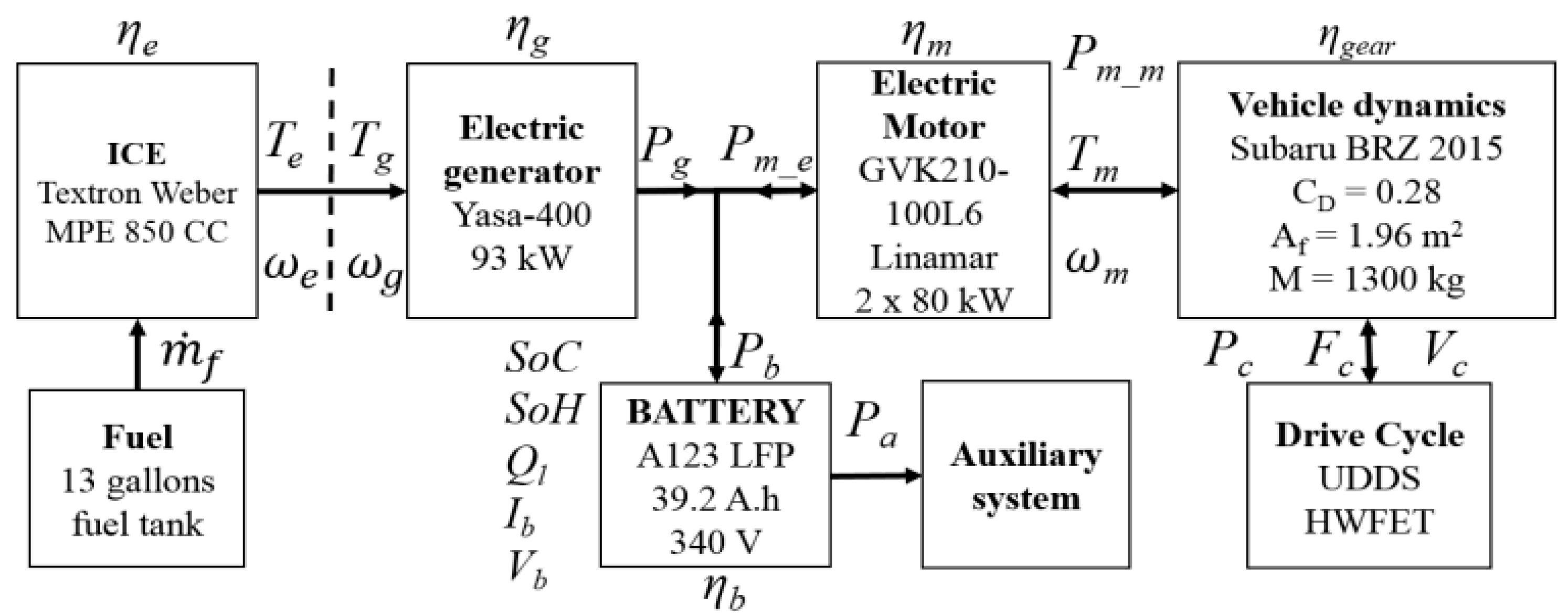
2.1. Overview
2.2. Vehicle Dynamics Model: State Space Equations
3. Model Predictive Control Strategy
3.1. Overview
3.2. Objective Function
3.3. Optimization Solver
4. Battery Models for the Sensitivity Analysis
4.1. Methodology
4.2. Development of Battery Models
4.3. Battery Dynamics Model Equations
4.4. Aging of Battery Models
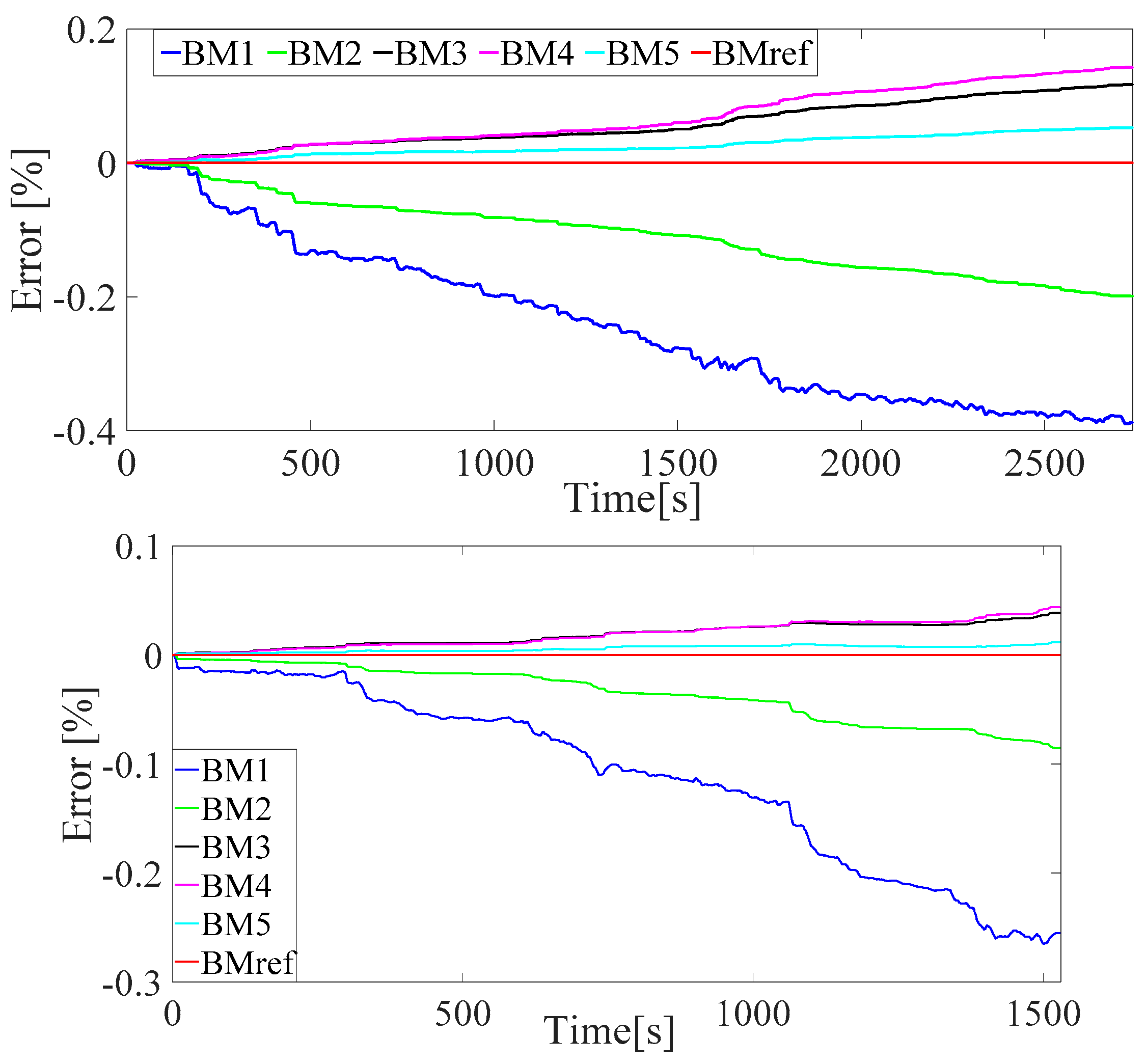
5. Simulation Results
- the electric generator power entirely dependent on the fuel consumption as shown in Figure 2,
- the auxiliary power defined as the same constant for the MPC model and the real vehicle,
- the electric motor power depending on its efficiency, the vehicle dynamics, and the speed profile, which are the same between the MPC model and the real vehicle.
6. Conclusions
Author Contributions
Funding
Conflicts of Interest
Nomenclature
| Symbol | Name | Units |
| Discrete time | [s] | |
| Step time | [s] | |
| X | State variables | - |
| U | Control input | - |
| W | Disturbance vector | - |
| Rolling resistance | [N] | |
| Grading resistance | [N] | |
| Aerodynamic drag resistance | [N] | |
| Acceleration ristance | [N] | |
| Sum of every resistant force applied to the car | [N] | |
| Power provided by the battery | [W] | |
| Electric power requested by the motor | [W] | |
| Power provided by the generator | [W] | |
| Constant power consumed by the auxiliary electric system | [W] | |
| Power provided by the battery | [W] | |
| Power requested by the car | [W] | |
| Mechanical power provided by the motor | [W] | |
| Car speed | [m/s] | |
| Caacceleration | [m/s2] | |
| Earth gravitational constant | [m/s2] | |
| Motor speed | [rads/s] | |
| Generator speed | [rads/s] | |
| Engine speed | [rads/s] | |
| Generator torque | [N.m] | |
| Engine torque | [N.m] | |
| Motor torque | [N.m] | |
| Sum of the engine and generator flywheel moment of inertia | [kg/m2] | |
| Inertia mass due to all rotating parts | [kg] | |
| Car mass | [kg] | |
| Battery coulomb efficiency | - | |
| Generator efficiency | - | |
| Motor gear ratio efficiency | - | |
| Motor efficiency | - | |
| Enge efficiency | - | |
| Battery voltage | [V] | |
| Battery open circuit voltage | [V] | |
| RS | Series resistance | [Ω] |
| RT_S | Short transient voltage response resistance | [Ω] |
| CT_S | Short transient voltage response capacitance | [F] |
| RT_L | Long transient voltage response resistance | [Ω] |
| CT_L | Long transient voltage response capacity | [F] |
| Current provided/received by the battery | [A] | |
| Battery State of Charge | - | |
| Nominal battery capacity | [A.h] | |
| Battery capacity fades | - | |
| ΔSoC | Equivalent cumulative SoC variation for a given Crate | - |
| Nominal energy capacity of the battery | [J] | |
| End of life percentage of a battery for EVs | - | |
| End of life percentage of a battery for stationary applications | ||
| Cradle-to-gate embodied primary energy per unit of electrical energy capacity for lithium battery | - | |
| Energy density of the fuel | [J/kg] | |
| Energy cost function | [J] | |
| Instant fuel consumption | [kg/s] | |
| Car static rolling coefficient | - | |
| Car dynamic rolling coefficient | - | |
| Car drag coefficient | - | |
| Gear reduction | - | |
| Wheels radius | [m] | |
| Car front size surface | [m2] | |
| Air density | [kg/m3] | |
| R | Perfect gas constant | [J/mol·K] |
| Ea | Activation energy | J/mol |
| z | Power law factor | - |
| B | Pre-exponent factor | - |
References
- Shahverdi, M.; Mazzola, M.S.; Grice, Q.; Doude, M. Pareto Front of Energy Storage Size and Series HEV Fuel Economy Using Bandwidth-Based Control Strategy. IEEE Trans. Transp. Electr. 2016, 2, 36–51. [Google Scholar] [CrossRef]
- Shahverdi, M.; Mazzola, M.; Grice, Q.; Doude, M. Bandwidth-Based Control Strategy for a Series HEV with Light Energy Storage System. IEEE Trans. Veh. Technol. 2016, 66, 1040–1052. [Google Scholar] [CrossRef]
- Overall Objectives of Model Predictive Control. Course of the University of California. Available online: https://chemengr.ucsb.edu/~ceweb/faculty/seborg/teaching/SEM_2_slides/Chapter_20%203-6-05.pdf (accessed on 19 March 2017).
- Qin, S.J.; Thomas, A.B. A survey of industrial model predictive control technology. Control Eng. Pract. 2003, 11, 733–764. [Google Scholar] [CrossRef]
- Malikopoulos, A. Supervisory power management control algorithms for hybrid electric vehicles: A survey. IEEE Trans. Intell. Transp. Syst. 2014, 15, 1869–1885. [Google Scholar] [CrossRef]
- Kermani, S.; Delprat, S.; Guerra, T.M.; Trigui, R. Predictive Control for HEV Energy Management: Experimental Results. In Proceedings of the IEEE Vehicle Power and Propulsion Conference (VPPC), Dearborn, MI, USA, 7–11 September 2009. [Google Scholar]
- Yu, K.; Xu, X.; Liang, Q.; Hu, Z.; Yang, J.; Guo, Y.; Zhang, H. Model Predictive Control for Connected Hybrid Electric Vehicle. Math. Probl. Eng. 2015, 2015. [Google Scholar] [CrossRef]
- Shahverdi, M.; Mazzola, M.; Abdelwahed, S.; Doude, M.; Zhu, D. MPC-based power management system for a plug-in hybrid electric vehicle for relaxing battery cycling. In Proceedings of the IEEE Transportation Electrification Conference and Expo (ITEC), Chicago, IL, USA, 27–29 June 2016. [Google Scholar]
- Di Cairano, S.; Liang, W.; Kolmanovsky, I.V.; Kuang, M.L.; Phillips, A.M. Power smoothing energy management and its application to a series hybrid powertrain. IEEE Trans. Control Syst. Technol. 2013, 21, 2091–2103. [Google Scholar] [CrossRef]
- Patil, R.M.; Filipi, Z.; Fathy, H.K. Comparison of Supervisory Control Strategies for Series Plug-In Hybrid Electric Vehicle Powertrains through Dynamic Programming. IEEE Trans. Control Syst. Technol. 2014, 22, 502–509. [Google Scholar] [CrossRef]
- Yan, F.; Wang, J.; Huang, K. Hybrid electric vehicle model predictive control torque-split strategy incorporating engine transient characteristics. IEEE Trans. Veh. Technol. 2012, 61, 2458–2467. [Google Scholar] [CrossRef]
- Patil, R.M.; Kelly, J.C.; Filipi, Z.; Fathy, H.K. A Framework for the Integrated Optimization of Charging and Power Management in Plug-in Hybrid Electric Vehicles. IEEE Trans. Veh. Technol. 2013, 62, 2402–2412. [Google Scholar] [CrossRef]
- Malikopoulos, A.A.; Smith, D.E. An optimization model for plug-in hybrid electric vehicles. In Proceedings of the ASME Internal Combustion Engine Division Fall Technical Conference, Morgantown, WV, USA, 2–5 October 2011. [Google Scholar]
- Mayne, D.Q.; Rawlings, J.B. Model Predictive Control: Theory and Design; Nob Hill Publishing, LLC: Madison, WI, USA, 2009. [Google Scholar]
- Yip, W.S.; Marlin, T.E. The Effect of Model Fidelity on Real-time Optimization Performance. Comput. Chem. Eng. 2004, 28, 267–280. [Google Scholar] [CrossRef]
- Nafsun, A.I.; Yusoff, N. Effect of Model-Plant Mismatch on MPC Controller Performance. J. Appl. Sci. 2011, 148, 3579–3585. [Google Scholar] [CrossRef]
- Badwe, A.S.; Shah, S.L.; Patwardhan, S.C.; Patwardhan, R.S. Model-Plant Mismatch Detection in MPC Applications using Partial Correlation Analysis. IFAC Proc. 2008, 41, 14926–14933. [Google Scholar] [CrossRef]
- Tufa, L.D.; Ka, C.Z. Effect of Model Plant Mismatch on MPC Performance and Mismatch Threshold Determination. In Proceedings of the 4th International Conference on Process Engineering and Advanced Materials, Kuala Lumpur, Malaysia, 15–17 August 2016; pp. 1008–1014. [Google Scholar]
- Patwardhan, R.S.; Shah, S.L. Issues in performance diagnostics of model-based controllers. J. Process Control 2002, 12, 413–427. [Google Scholar] [CrossRef]
- Badwe, A.S.; Patwardhan, R.S.; Shah, S.L.; Patwardhan, S.C.; Gudi, R.D. Quantifying the impact of model-plant mismatch on controller performance. J. Process Control 2010, 20, 408–425. [Google Scholar] [CrossRef]
- Ahmad, M.W.; Eftekhari, M.; Steffen, T.; Rowley, P. The Effect of Model and Objective Function Mismatch in Model Predictive Control (MPC) for a Solar Heating System with a Heat Pump. In Proceedings of the 2014 UKACC International Conference on Control, Loughborough, UK, 9–11 July 2014. [Google Scholar]
- Liu, J.; Jayakumar, P.; Stein, J.L.; Ersal, T. A study on model fidelity for model predictive control-based obstacle avoidance in high-speed autonomous ground vehicles. Veh. Syst. Dyn. 2016, 54, 1629–1650. [Google Scholar] [CrossRef]
- Michael, M.; Masood, S. Li-Ion Battery Pack and Applications. In Rechargeable Batteries; Springer International Publishing: Cham, Switzerland, 2015; pp. 455–476. [Google Scholar]
- Nicolas, S.; Jian, S.; Masood, S.; Michael, M. Sensitivity analysis of the battery model for model predictive control implemented into a plug-in hybrid electric vehicle. In Proceedings of the IEEE Transportation Electrification Conference and Expo (ITEC), Chicago, IL, USA, 22–24 June 2017. [Google Scholar]
- Sockeel, N.; Shahverdi, M.; Mazzola, M.; Meadows, W. High-Fidelity Battery Model for Model Predictive Control Implemented into a Plug-In Hybrid Electric Vehicle. Batteries 2017, 3, 13. [Google Scholar] [CrossRef]
- Nicolas, S.; Jian, S.; Masood, S.; Michael, M. Pareto front analysis of the objective function in model predictive based power management system of a plug-in hybrid electric vehicle. In Proceedings of the IEEE Transportation Electrification Conference and Expo (ITEC), Long Beach, CA, USA, 13–15 June 2018. [Google Scholar]
- Nicolas, S.; Jian, S.; Masood, S.; Michael, M. Sensitivity analysis of the vehicle model mass for model predictive based power management system of a plug-in hybrid electric vehicle. In Proceedings of the IEEE Transportation Electrification Conference and Expo (ITEC), Long Beach, CA, USA, 13–15 June 2018. [Google Scholar]
- Charles, J.; Benson, S.M. On the importance of reducing the energetic and material demands of electrical energy storage. Energy Environ. Sci. 2013. [Google Scholar] [CrossRef]
- MathWorks. Fmincon. 2018. Available online: https://www.mathworks.com/help/optim/ug/fmincon.html (accessed on 31 October 2018).
- Bai, J.; Abdelwahed, S. Efficient Algorithms for Performance Management of Computing Systems. In Proceedings of the IEEE Fourth International Workshop on Feedback Control Implementation and Design in Computing Systems and Networks (FeBID), San Francisco, CA, USA, April 2009. [Google Scholar]
- Meyer, R.; DeCarlo, R.A.; Meckl, P.H.; Doktorcik, C.; Pekarek, S. Hybrid Model Predictive Power Flow Control of a Fuel Cell-Battery Vehicle. In Proceedings of the IEEE American Control Conference, San Francisco, CA, USA, 29 June–1 July 2011. [Google Scholar]
- Einhorn, M.; Conte, F.V.; Kral, C.; Fleig, J. Comparison, Selection, and Parametrization of Electrical Battery Models for Automotive Applications. IEEE Trans. Power Electron. 2013, 28, 1429–1437. [Google Scholar] [CrossRef]
- He, H.; Xiong, R.; Fan, J. Evaluation of Lithium-Ion Battery Equivalent Circuit Model for State of Charge Estimation by an Experimental Approach. Energies 2011, 4, 582–598. [Google Scholar] [CrossRef]
- Chen, M.; Rincon-Mora, G.A. Accurate Electrical Battery Model Capable of Predicting Runtime and I-V Performance. IEEE Trans. Energy Convers. 2006, 21, 504–511. [Google Scholar] [CrossRef]
- Orcioni, S.; Buccolini, L.; Ricci, A.; Conti, M. Lithium-ion Battery Electrothermal Model, Parameter Estimation, and Simulation Environment. Energies 2017, 10, 375. [Google Scholar] [CrossRef]
- Cicconi, P.; Germani, M.; Landi, D.; Mengarelli, M. Virtual Prototyping Approach to Evaluate the Thermal Management of Li-Ion Batteries. In Proceedings of the 2014 IEEE Vehicle Power and Propulsion Conference (VPPC), Coimbra, Portugal, 27–30 October 2014. [Google Scholar]
- Li, J.; Mazzola, M.S. Accurate battery pack modeling for automotive applications. J. Power Sources 2013, 237, 215–228. [Google Scholar] [CrossRef]
- Sockeel, N.; Ball, J.; Shahverdi, M.; Mazzola, M. Passive tracking of the electrochemical impedance of a hybrid electric vehicle battery and state of charge estimation through an extended Kalman filter. In Proceedings of the IEEE Transportation Electrification Conference and Expo (ITEC), Chicago, IL, USA, 22–24 June 2017. [Google Scholar]
- Sockeel, N.; Ball, J.; Shahverdi, M.; Mazzola, M. Passive tracking of the electrochemical impedance of a hybrid electric vehicle battery and state of charge estimation through an extended and unscented Kalman filter. Batteries 2018, 4, 52. [Google Scholar] [CrossRef]
- Wang, J.; Liu, P.; Hicks-Garner, J.; Sherman, E.; Soukiazian, S.; Verbrugge, M.; Tataria, H.; Musser, J.; Finamore, P. Cycle-life model for graphite-LifePO4 cells. J. Power Sources 2010, 196, 3942–3948. [Google Scholar] [CrossRef]
- MathWorks. Polyval. 2018. Available online: https://www.mathworks.com/help/matlab/ref/polyval.html?searchHighlight=polyval&s_tid=doc_srchtitle (accessed on 31 October 2018).
- MathWorks. Polyfit. 2018. Available online: https://www.mathworks.com/help/matlab/ref/polyfit.html?searchHighlight=polyfit&s_tid=doc_srchtitle (accessed on 31 October 2018).
- MathWorks. Interp1. 2018. Available online: https://www.mathworks.com/help/matlab/ref/interp1.html?searchHighlight=interp1&s_tid=doc_srchtitle (accessed on 31 October 2018).


| Power-Train Components | Name | Characteristics |
|---|---|---|
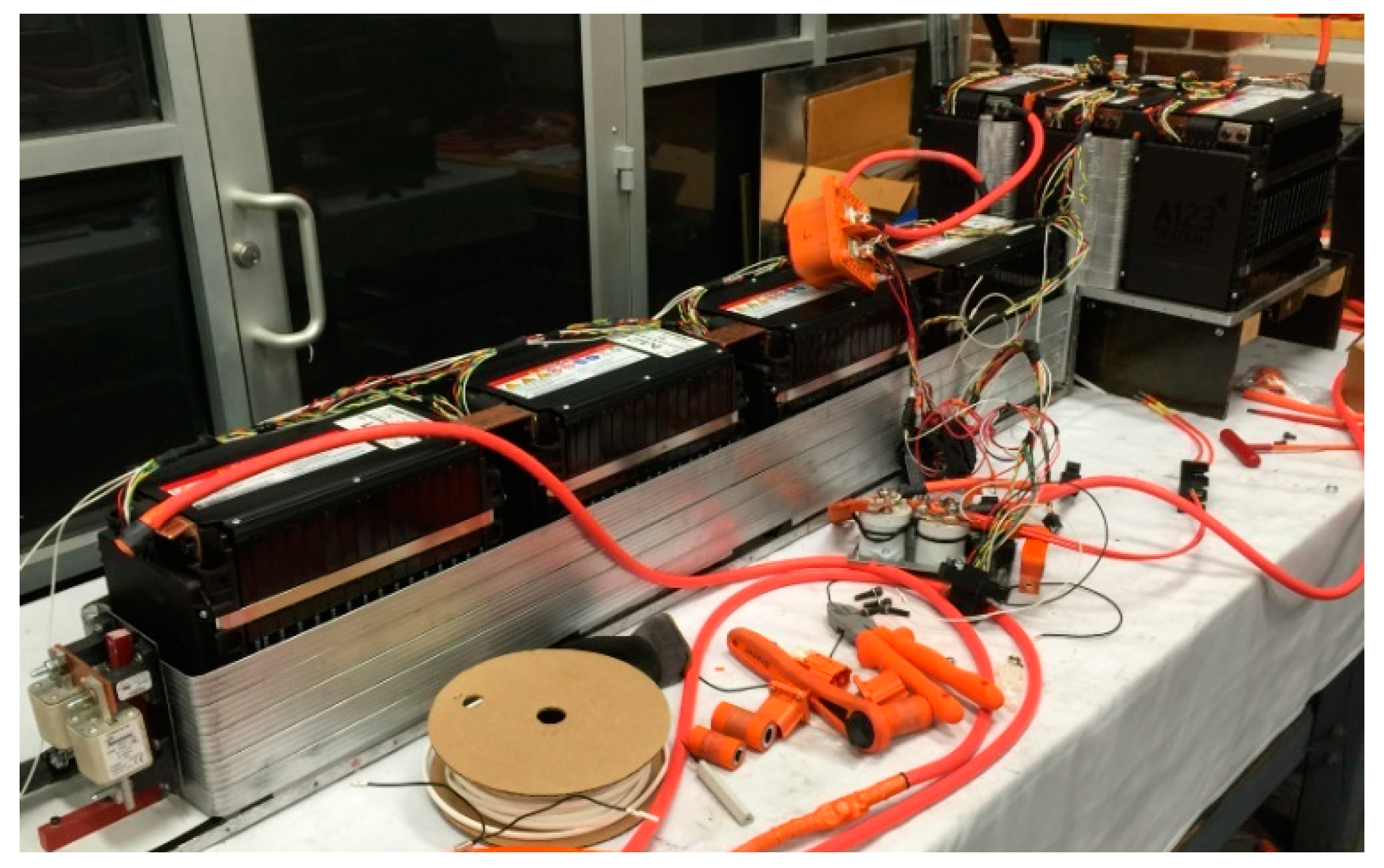
| Energy Storage System (ESS) | Lithium iron phosphate (LFP) prismatic cells from A123 | Capacity = 39.2 Ah; nominal voltage = 340 V; nominal energy = 13.3 kWh; configuration: 7×15s2p. |
| Internal Combustion Engine (ICE) | Model MPE850 from Weber | 41 kW, 2 cylinders, 850 cc. |
| Electric Generator | Model YASA-400 | 93 kW, axial flux permanent magnet. |
| Electric Motors Unit | Model GVK210-100L6 from Linamar | 2 × 80 kW, unit ratio = 8.49. |
| Vehicle dynamics | 2015 Subaru BRZ Limited | Drag coefficient = 0.28; frontal area = 1.9695 m2; PHEV mass = 1300 kg; wheel radius = 0.3 m. |
| Name | Notation | Value |
|---|---|---|
| Algorithm type | Algorithm | Interior-point |
| Step tolerance | TolX | 1 |
| Function tolerance | TolFun | 0.01 |
| Maximum Iteration | MaxIter | 1000 |
| Maximum Function Evaluation | MaxFunEval | 1000 |
| Constraint Tolerance | TolCon | 0.1 |
| Name | BM1 | BM2 | BM3 | BM4 | BM5 | BMref |
|---|---|---|---|---|---|---|
| Voc (V) | 350 | g(SoC) | ||||
| RS (Ω) | 0 | 0 | 0.15 | f(SoC) | 0.095 | 0.1094 |
| RT_S (Ω) | 0 | 0 | 0 | 0 | 0.0118 | 0.1111 |
| CT_S (F) | 0 | 0 | 0 | 0 | 287.8 | 422.7 |
| RT_L (Ω) | 0 | 0 | 0 | 0 | 0 | 0.1115 |
| CT_L (F) | 0 | 0 | 0 | 0 | 0 | 10,196 |
| Function | BM1 | BM2 | BM3 | BM4 | BM5 | BMref | |
|---|---|---|---|---|---|---|---|
| Ib | - | 1 | 1 | 9 | 9 | 1 | 1 |
| Voc | “Polyfit” | - | 936 | 936 | 936 | 936 | 936 |
| “Polyval” | - | 31 | 31 | 31 | 31 | 31 | |
| Vb | - | - | - | 2 | 2 | 3 | 4 |
| Rs | “Interp1” | - | - | - | 10 | - | - |
| VT_S | - | - | - | - | - | 4 | 4 |
| VT_L | - | - | - | - | - | - | 4 |
| Total Computation Cost | 1 | 968 | 978 | 988 | 975 | 980 | |
| Computation time | 512 s | 919 s | 921 s | 977 s | 903 s | 909 s | |
| Simulation time | 2740 s | 2740 s | 2740 s | 2740 s | 2740 s | 2740 s | |
| Battery model computation time | 0.0097 s | 0.0170 s | 0.0170 s | 0.0180 s | 0.0168 s | 0.0169 s | |
© 2018 by the authors. Licensee MDPI, Basel, Switzerland. This article is an open access article distributed under the terms and conditions of the Creative Commons Attribution (CC BY) license (http://creativecommons.org/licenses/by/4.0/).
Share and Cite
Sockeel, N.; Shi, J.; Shahverdi, M.; Mazzola, M. Sensitivity Analysis of the Battery Model for Model Predictive Control: Implementable to a Plug-In Hybrid Electric Vehicle. World Electr. Veh. J. 2018, 9, 45. https://doi.org/10.3390/wevj9040045
Sockeel N, Shi J, Shahverdi M, Mazzola M. Sensitivity Analysis of the Battery Model for Model Predictive Control: Implementable to a Plug-In Hybrid Electric Vehicle. World Electric Vehicle Journal. 2018; 9(4):45. https://doi.org/10.3390/wevj9040045
Chicago/Turabian StyleSockeel, Nicolas, Jian Shi, Masood Shahverdi, and Michael Mazzola. 2018. "Sensitivity Analysis of the Battery Model for Model Predictive Control: Implementable to a Plug-In Hybrid Electric Vehicle" World Electric Vehicle Journal 9, no. 4: 45. https://doi.org/10.3390/wevj9040045
APA StyleSockeel, N., Shi, J., Shahverdi, M., & Mazzola, M. (2018). Sensitivity Analysis of the Battery Model for Model Predictive Control: Implementable to a Plug-In Hybrid Electric Vehicle. World Electric Vehicle Journal, 9(4), 45. https://doi.org/10.3390/wevj9040045