Physics-Informed Feature Analysis and Exploratory Clustering of Electric Vehicle On-Board Charger Behaviour

Abstract

Electric vehicle (EV) smart charging changes the operating point of the vehicle on-board charger (OBC), so conversion efficiency and grid-side power quality can vary materially with the charging current. This study reanalyses an experimental dataset of 38 EV models represented by 39 test units manufactured between 2011 and 2022. The source study established the measured current-dependent efficiency and reactive-power behaviour; the present work extends those measurements through vehicle-level physics-informed loss decomposition, a 24-variable descriptive feature set, formal statistical comparisons, exploratory clustering with stability analysis, and annual energy scenario sensitivity. A three-component loss model separating fixed, current-proportional, and ohmic effects reproduced the measured efficiency curves with a median root mean square error of 0.22 percentage points. For clustering, an exact redundant efficiency descriptor was removed, and eight variables were retained. Stage 1 separated four motor-winding-integrated chargers from 32 dedicated OBCs (silhouette coefficient 0.474; Ward adjusted Rand index 1.00). The finer four-way partition of the dedicated OBC subset had a lower silhouette coefficient of 0.324 and showed substantial bootstrap sensitivity; it is therefore reported as exploratory rather than as a universal OBC typology. Peak efficiency increased by 0.53 percentage points per model year, whereas the fitted fixed-loss coefficient showed no significant temporal trend. Across 21 paired vehicles, the mean same-current difference between the three-phase and curtailed single-phase operation was 6.32 percentage points; because total transferred power also changes with phase count, this value is not interpreted as an isolated causal phase effect. For a 2500 kWh/year battery-delivered reference demand, the minimum operation supported a current produced at an extreme-case fleet-average, with an additional conversion loss of approximately 190 kWh/year relative to operation at the most efficient measured set-point. Sensitivity analysis shows that the additional energy scales strongly with annual demand and with the fraction of energy charged at low current. The resulting vehicle-specific loss parameters provide a reproducible basis for OBC-aware smart-charging studies, while the dataset-derived behavioural groups require validation on independent vehicles and operating conditions.

1. Introduction

The global transition towards electric vehicles (EVs) increases the importance of alternating-current (AC) charging at homes and workplaces, where the vehicle on-board charger (OBC) is the final power–electronic conversion stage between the grid and the battery [1,2,3,4,5,6,7,8,9,10]. Its operating point determines not only AC-to-DC conversion efficiency but also power factor and reactive-power exchange. Smart-charging controllers deliberately vary the charging current to manage demand, tariffs, renewable energy availability, and network constraints [11,12,13,14,15,16]; consequently, they move each OBC along a vehicle-specific part-load characteristic rather than operating it at one rated efficiency. Low-current operation is particularly important because fixed converter and auxiliary losses are distributed over a smaller power throughput. Phase allocation can further change the operating condition of three-phase-capable vehicles [17,18]. Dedicated OBCs and motor-winding-integrated charging arrangements also differ in topology and control [7,19], so a fleet-average or constant-efficiency representation can obscure substantial vehicle-to-vehicle differences in efficiency, power factor, and reactive power. The experimental campaign of Sevdari et al. [20] is the empirical basis of this study. It reported charging-efficiency, power-factor, and reactive-power measurements for 38 EV models over current set-points from 6 A to 32 A and showed that current modulation can increase charging energy demand, particularly at low current, while some vehicles exhibit substantial reactive-power exchange. Those observations are therefore not claimed here as new experimental findings. Instead, the present work asks what additional, physically interpretable and statistically qualified information can be extracted from the published vehicle-resolved measurements. The present reanalysis extends Ref. [20] in four ways. First, each measured efficiency curve is represented by a constrained three-component loss model that separates fixed, current-proportional, and ohmic contributions. Second, the measured and fitted quantities are assembled into a unified 24-variable descriptive representation spanning efficiency, loss parameters, power factor, and reactive power. Third, the study quantifies model–year trends and the same-current three-phase versus curtailed single-phase difference using formal uncertainty and paired statistics. Fourth, it uses exploratory clustering to examine recurring behavioural groups and, in response to the limited sample size, evaluates their stability by Ward clustering, 1000-resample bootstrap analysis, leave-one-out reruns, small-group removal, and reduced-feature sensitivity. The finer groups are interpreted only as structures observed in this dataset.

The contributions to the literature are therefore:

• A vehicle-specific physics-informed loss representation and 24-variable electrical description that connect measured OBC efficiency curves with power-factor and reactive-power behaviour.
• A stability-qualified exploratory grouping analysis based on an eight-variable non-exact-redundant subset, with independent Ward comparison, bootstrap resampling, leave-one-out analysis, and feature/small-group sensitivity.
• Quantified technology trends, same-current three-phase versus curtailed single-phase differences, and annual energy sensitivity scenarios that indicate when OBC-aware charging models can materially change energy estimates.

The remainder of this article is organised as follows. Section 2 positions the reanalysis within the OBC literature and describes the DTU dataset, harmonisation, and analytical scope. Section 3 presents the loss model, descriptive features, statistical analyses, exploratory clustering and stability procedures, scenario sensitivity, and reproducibility materials. Section 4 reports and discusses the results with explicit attention to stability and external-validity limits. Section 5 provides the principal conclusions.

2. Literature Context and Experimental Dataset

2.1. State-of-the-Art and Positioning of the Present Reanalysis

Research on EV charging spans charging infrastructure, OBC converter design, smart-charging coordination, grid-impact assessment, and vehicle-side conversion measurements [1,2,3,4,5,6,7,8,9,10,11,12,13,14,15,16,17,18,19]. Dedicated OBCs typically combine a grid-side power-factor-correction stage with DC-DC conversion, whereas integrated arrangements may reuse traction system components [4,5,6,7,8,9,10,19]. These topology studies explain the physical origins of fixed, proportional, switching, and ohmic losses, but they commonly evaluate prototypes or restricted operating points rather than a broad set of production vehicles. Smart-charging studies demonstrate the operational value of current modulation for peak management, flexibility, and renewable energy integration [2,11,17,18]. However, optimisation formulations frequently use constant or vehicle-independent charging efficiency. That simplification is most consequential at low power, where fixed losses become proportionally larger. Independent experimental work has likewise shown that power–electronic efficiency is lower at low power transfer [9]. Phase allocation and load-balancing studies focus mainly on network imbalance, conductor loading, and voltage effects [12,13,14,15,16]. When a three-phase-capable vehicle is operated in a curtailed single-phase mode at the same per-phase current, total transferred power is approximately one third of the corresponding three-phase value, so any efficiency difference combines phase configuration with the ordinary effect of lower total throughput. The present paper therefore reports this quantity as a same-current configuration difference rather than as a pure phase effect.

The vehicle-resolved campaign of Sevdari et al. [20] is especially relevant because it measured efficiency, power factor, and reactive power for a broad production–EV sample across multiple current set-points. Ref. [20] already established the low-current efficiency and reactive-power behaviour of the measured vehicles. The present study does not repeat that novelty claim; it adds physics-informed parameterisation, integrated feature construction, formal trend and paired analyses, exploratory behavioural grouping with resampling stability tests, and scenario sensitivity.

The literature supports a physically interpretable analysis of OBC behaviour but also establishes two constraints on the present reanalysis: low-current inefficiency is already an empirical finding in the source study, and a grouping derived from one experimental corpus cannot be assumed to generalise to unseen vehicles. Accordingly, the current contribution is framed as a reanalysis that quantifies and organises the measured behaviour rather than as external validation of a universal OBC classification. The analysis therefore uses the DTU measurements to estimate vehicle-specific loss parameters, descriptive electrical features, trend statistics, same-current configuration differences, and exploratory behavioural groups. The latter are accompanied by explicit stability analyses and are treated as dataset-derived structures whose external validity remains to be tested.

2.2. Data Source and Experimental Scope

This study uses the open experimental dataset entitled Experimental Validation of Onboard Electric Vehicle Chargers to Improve the Efficiency of Smart Charging Operation, published through DTU Data under DOI: 10.11583/DTU.25425262 and released in conjunction with the experimental investigation by Sevdari et al. [20]. The dataset provides vehicle-resolved measurements of electric vehicle (EV) on-board charger (OBC) performance under controlled alternating-current charging conditions. Unlike charging session datasets that report only energy consumption, connection duration, or charging-station utilisation, this dataset directly characterises the electrical behaviour of the vehicle-side power-conversion stage across multiple charging-current set-points. The source data comprise five measurement matrices containing conversion efficiency, power factor, and per-phase reactive power under conventional three-phase and curtailed single-phase charging. Each matrix is indexed by vehicle and per-phase charging-current set-points, where

$$I\in \{6,8,\dots ,32\}\mathrm{A}.$$

The current set-points increase in 2 A increments, although the available range differs among vehicles according to the maximum AC charging current supported by the corresponding OBC. The three-phase matrices describe normal operation of three-phase-capable vehicles, whereas the curtailed matrices report the same electrical quantities when these vehicles are operated using only one phase. This paired measurement structure enables direct comparison of OBC behaviour under different phase configurations while retaining a common per-phase current reference. Conversion efficiency is defined in the original experimental campaign as the ratio of the direct-current power delivered to the battery to the alternating-current active power measured at the grid-side charging interface:

$$\eta ={\displaystyle \frac{P_{\mathrm{D}\mathrm{C}}}{P_{\mathrm{A}\mathrm{C}}}},$$

where $P_{\mathrm{D}\mathrm{C}}$ is the DC power delivered to the battery and $P_{\mathrm{A}\mathrm{C}}$ is the AC active power drawn by the vehicle. Power factor is reported as a dimensionless quantity, whereas reactive power is reported in var per phase. The simultaneous availability of efficiency, power-factor, and reactive-power measurements enables the OBC to be assessed as both an energy-conversion device and a grid-connected power–electronic load. The investigated vehicles span model years 2011–2022 and include conventional dedicated OBCs as well as vehicles employing motor-winding-integrated charging architectures. The dataset therefore captures differences associated with vehicle generation, converter topology, supported charging-current range, low-current operability, and phase configuration. These characteristics make it particularly suitable for examining whether production EVs exhibit recurring and electrically interpretable patterns of OBC behaviour. Following the harmonisation and quality-control procedures described in Section 2.2, the analytical corpus contains 39 independently measured test units representing 38 distinct EV models. The difference between the number of models and test units arises because two separate units of the 2017 VW e-Golf were experimentally evaluated. Valid conversion-efficiency measurements are available for 36 test units, while power-factor and reactive-power measurements are available for 38 test units. The Volvo XC40 Recharge and two Polestar 2 variants are represented only in the power quality matrices and do not contain corresponding efficiency measurements. Paired three-phase and curtailed single-phase efficiency measurements are available for 21 vehicles. The final three-phase dataset contains 311 valid efficiency observations, 294 power-factor observations, and 305 reactive-power observations. The curtailed single-phase dataset contains 213 efficiency observations, 246 power-factor observations, and 246 reactive-power observations. Differences among these totals reflect vehicle-specific current limits, unavailable measurements, and instances in which a vehicle could not sustain charging at a particular set-point. The dataset composition is summarised in

Table 1. Composition of the harmonised OBC measurement dataset.

Operating Configuration	Measurement Quantity	Test Units Represented	Valid Observations	Unit
Three-phase	Conversion efficiency	36	311	%
Three-phase	Power factor	38	294	-
Three-phase	Per-phase reactive power	38	305	var
Curtailed single-phase	Conversion efficiency	21 paired vehicles	213	%
Curtailed single-phase	Power factor	Three-phase-capable vehicles	246	-
Curtailed single-phase	Per-phase reactive power	Three-phase-capable vehicles	246	var

. The positioning of the source study, related OBC research, and the present reanalysis in tabulated in

Table 2. Positioning of the source study, related OBC research, and the present reanalysis.

Research Area	Refs.	What is Established	Remaining Issue for This Study	Role in Present Reanalysis
Charging systems and OBC architectures	[1,3,4,5,6,7,8,9,10,19]	Converter requirements, topology and physical loss mechanisms	Often prototype/rated-point focused	Physical basis for loss decomposition
Smart charging and flexibility	[2,11,17,18]	Current modulation, scheduling and flexibility value	Efficiency often simplified as constant	Motivates vehicle-specific efficiency functions
Phase allocation/load balancing	[12,13,14,15,16]	Network effects of phase choice and current allocation	Phase count and total-power effects can be confounded	Same-current comparison is explicitly scope-qualified
Independent loss measurements	[9]	Low-power transfer can reduce power–electronic efficiency	Different vehicles/conditions; not a validation set for the DTU groups	Provides qualitative external consistency only
DTU source experiment	[20]	Vehicle-resolved efficiency, PF and Q across current set-points; low-current losses already demonstrated	No physics-informed loss decomposition or resampling stability analysis	Primary measurement corpus for the present reanalysis
Present reanalysis	-	Loss parameters, 24 descriptive variables, formal trend/paired statistics, exploratory grouping and scenario sensitivity	Single source dataset; fine grouping has limited stability	Scope-qualified, reproducible feature-level analysis

.

The measurements were transformed into a long-form analytical structure in which each row represents one test unit, one phase configuration, and one charging-current set-point. Vehicle identity, manufacturer, model, model year, phase configuration, current set-point, efficiency, power factor, and reactive power were retained as separate fields. This structure preserves the vehicle-specific nature of the measurements and prevents observations from different vehicles or operating configurations from being inadvertently pooled.

2.3. Data Harmonisation and Quality Control

The five original measurement matrices were not directly suitable for integrated analysis because vehicle identifiers and model descriptions were inconsistent across files. Documented examples include “Renault Zoe50N (2021)” versus “Renault Zoe ZE50 R110 (2021)”, inconsistent Nissan LEAF naming, and the manufacturer typographical error “Hyudai”. Vehicle, variant, and model–year labels were therefore harmonised before matrix merging. Independently tested duplicate physical units were retained separately and assigned [A] and [B] suffixes. The analysis-label mapping used for the feature-level stability and sensitivity analyses is supplied with the reproducibility package.

QC1: Physically inadmissible power-factor values: Power factor must satisfy.

$$0\le \mathrm{P}\mathrm{F}\le 1.$$

Accordingly, values greater than unity were classified as physically inadmissible and removed. One such observation was identified for the 2022 VW ID.3 Pro at a current set-point of 20 A, where the reported power factor was 90.16. Because this value lies within the numerical range expected for conversion efficiency rather than power factor, it was interpreted as a probable cross-sheet transcription error. The value was therefore excluded from the power quality dataset and was not imputed.

QC2: Zero-efficiency entries representing non-sustained charging. Efficiency values equal to zero were not interpreted as physically measured zero-efficiency conversion events. A true efficiency of zero would imply that the vehicle continuously drew AC power while delivering no DC power to the battery, which was inconsistent with the structure of the reported measurements. These entries were therefore interpreted as indicators that the vehicle could not initiate or sustain charging at the corresponding current set-point.

This condition occurred at 6 A for the Renault Zoe R90, both Renault Zoe ZE50 test units, and the Nissan Townstar. These vehicles employ motor-winding-integrated charging arrangements, and their inability to maintain charging at the minimum set-point represents an important operating characteristic rather than a conventional missing value. The zero entries were excluded from efficiency curve fitting and from calculations requiring a valid operating efficiency. However, their information content was preserved through the binary fails-at-6 A feature and the minimum-operable-current feature.

QC3: Retention of independently measured duplicate models: The two 2017 VW e-Golf test units were retained as independent experimental observations rather than averaged into a single model-level curve. Their measured peak efficiencies were 88.40% and 88.44%, while the mean absolute difference between their efficiency curves was 0.31 percentage points. The close agreement provides an internal indication of repeatability and supports the treatment of vehicle-level curve characteristics as reproducible electrical descriptors. Nevertheless, the pair does not provide a sufficient sample for estimating general manufacturing variability across the wider vehicle population.

No interpolation or general statistical imputation was applied to the original measurement matrices. Missing cells were retained as unavailable observations because they predominantly reflect differences in the maximum supported charging current or the availability of a particular measurement quantity rather than random data loss. Each vehicle was therefore analysed only over its experimentally observed operating range. Median imputation subsequently used for a small number of missing power quality features during clustering is described separately in Section 3 and does not modify the underlying experimental measurements. The harmonisation and quality-control workflow produced cleaned measurement matrices and a long-form analytical dataset in which each exclusion or identifier correction was logged. The supplementary reproducibility package supplies the analysis-ready vehicle-feature table and analysis-label map used for the resampling and sensitivity analyses, allowing the feature-level clustering results to be independently reproduced from the reported inputs.

2.4. Analytical Scope and Limitations

The principal advantage of the DTU dataset is that OBC performance is measured over a sequence of controlled current set-points rather than represented by a single rated-power or peak-efficiency value. Consequently, each vehicle is described by an experimentally observed efficiency curve and corresponding power quality trajectories. This permits analysis of low-current losses, current-dependent efficiency variation, minimum operable current, power-factor deterioration, reactive-power magnitude, and phase-curtailment sensitivity. The dataset also supports a physics-informed representation of OBC losses. For a vehicle operating at current set-point $I$, the measured efficiency curve can be represented using the three-term model, $\eta \left(I\right)=1-\left({\displaystyle \frac{a}{I}}+b+cI\right),$ where $a$ represents the contribution of fixed losses, $b$ represents the current-proportional loss component, and $c$ represents the ohmic loss component. The availability of repeated efficiency measurements across the current range permits these parameters to be estimated separately for each vehicle rather than assumed to be identical across the fleet.

The combination of efficiency, power factor, and reactive power is also important because these quantities describe different aspects of OBC operation. High conversion efficiency does not necessarily imply favourable grid-side behaviour. An OBC may deliver a large proportion of the drawn active power to the battery while simultaneously exhibiting a reduced power factor or substantial reactive-power exchange. Conversely, an OBC with near-unity power factor may still exhibit considerable part-load conversion losses. A multidimensional feature representation is therefore required to characterise the complete electrical behaviour of the charger. The paired curtailed measurements provide a further analytical advantage because the same vehicle is observed under three-phase and curtailed single-phase operation at common per-phase current set-points. The resulting within-vehicle comparison reduces confounding from vehicle architecture and rated charging capability. However, it does not hold total transferred power constant: at the same per-phase current, single-phase operation transfers approximately one third of the power of the corresponding three-phase case. The paired statistic is therefore used as a same-current configuration comparison and is not interpreted as an isolated causal effect of phase count. The dataset remains a cross-sectional experimental corpus from one measurement campaign rather than an independent multi-site validation set. Most models are represented by one test unit, the measurements correspond to controlled steady-state operating points, and state of charge (SOC), ambient and battery temperature, grid-voltage variation, ageing, and manufacturing variability are not comprehensively resolved. Consequently, the loss parameters describe the measured units under the reported conditions, and the exploratory behavioural groups must not be interpreted as a definitive classification of all vehicles of the same model or topology.

3. Materials and Methods

The analytical workflow is shown in Figure 1. The sequence is deliberately ordered so that data harmonisation precedes vehicle-level loss fitting; fitted loss coefficients and directly measured descriptors are then assembled into the descriptive feature matrix; statistical analyses, exploratory clustering, stability tests, same-current configuration comparison, and annual energy sensitivity are applied only after feature construction.

3.1. Physics-Informed Loss Model and Feature Construction

• AC input power and conversion efficiency

Let $m$ denote the number of active phases, $V$ the root-mean-square phase voltage, $I$ the per-phase charging-current set-point, and $\cos \varphi$ the displacement power factor. The grid-side AC active power drawn by the OBC is expressed as

$$P_{\mathrm{A}\mathrm{C}}=mVI\mathrm{c}\mathrm{o}\mathrm{s} \varphi .$$

(1)

Following the definition adopted in the original experimental campaign, conversion efficiency is the ratio of the DC power delivered to the battery, $P_{\mathrm{D}\mathrm{C}}$, to the AC active power drawn at the measurement point, $P_{\mathrm{A}\mathrm{C}}$. Equivalently, efficiency may be expressed in terms of the total converter loss, $P_{\mathrm{l}\mathrm{o}\mathrm{s}\mathrm{s}}$, as

$$\eta ={\displaystyle \frac{P_{\mathrm{D}\mathrm{C}}}{P_{\mathrm{A}\mathrm{C}}}}=1-{\displaystyle \frac{P_{\mathrm{l}\mathrm{o}\mathrm{s}\mathrm{s}}}{P_{\mathrm{A}\mathrm{C}}}}.$$

(2)

The measured efficiency values were converted from percentages to per-unit quantities before model fitting. The resulting root mean square error values were subsequently converted back to percentage points to preserve direct engineering interpretation.

• Converter-loss decomposition

The total OBC loss was represented using the classical quadratic loss model

$$P_{\mathrm{l}\mathrm{o}\mathrm{s}\mathrm{s}}=P_0+k_1{P}_{\mathrm{A}\mathrm{C}}+k_2{P}_{\mathrm{A}\mathrm{C}}^2,$$

(3)

where $P_0$ represents approximately fixed losses associated with control electronics, gate drives, magnetic components, auxiliary systems, and cooling overheads. The coefficient $k_1$ represents losses that scale approximately in proportion to converter throughput, including semiconductor conduction and switching contributions, whereas $k_2$ represents predominantly ohmic losses associated with windings, filters, connectors, and cabling. Substituting Equation (3) into Equation (2), and applying Equation (1) under approximately constant phase voltage and displacement factor, gives an efficiency model expressed directly in terms of the controllable per-phase current set-point:

$$\eta (I)=1-\left({\displaystyle \frac{a}{I}}+b+cI\right),a,b,c\ge 0.$$

(4)

The model coefficients are related to the underlying loss terms through

$$a={\displaystyle \frac{P_0}{mV\mathrm{c}\mathrm{o}\mathrm{s} \varphi }},b=k_1,c=k_{2}mV\mathrm{c}\mathrm{o}\mathrm{s} \varphi .$$

(5)

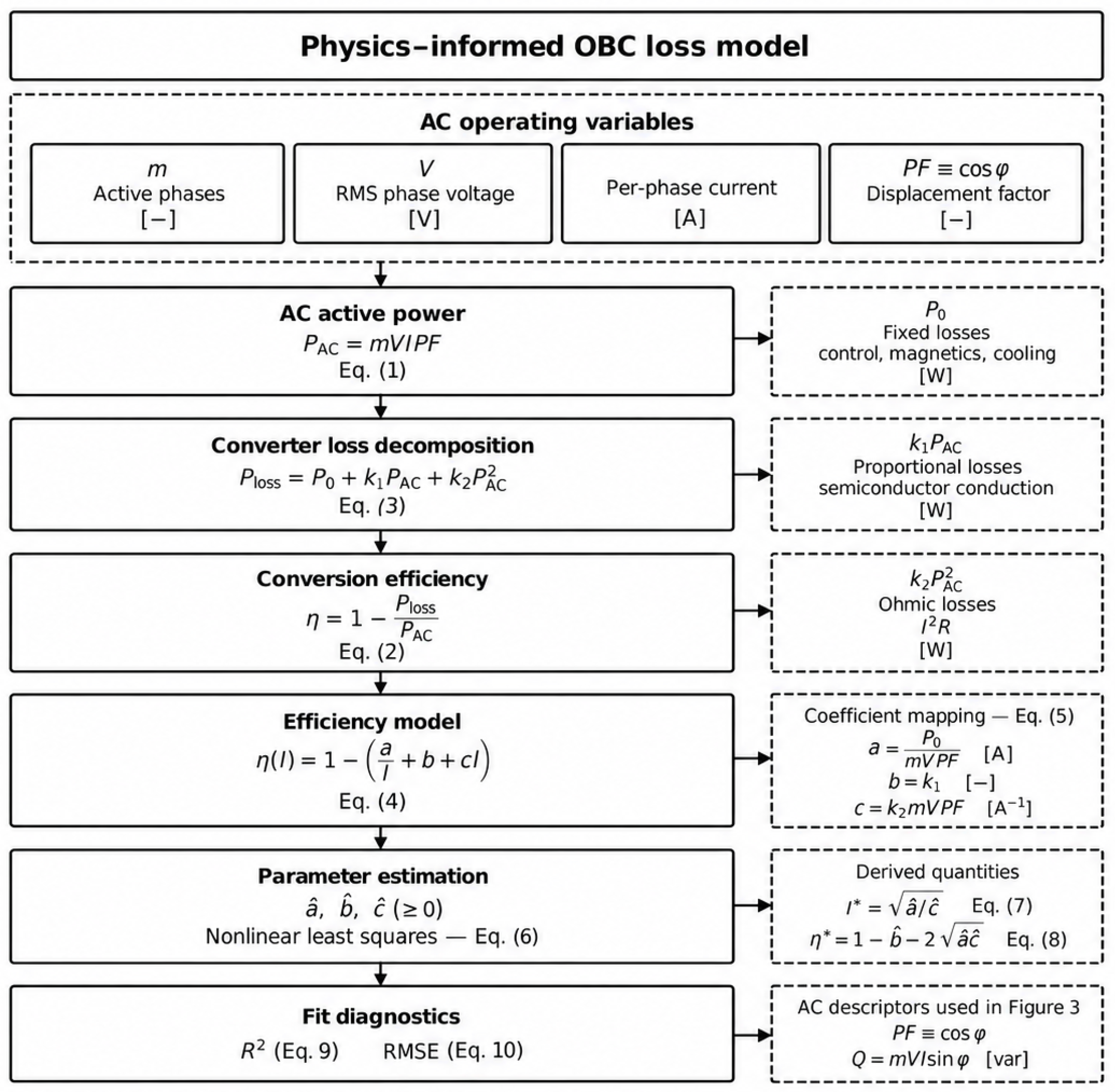
The coefficient $a$ has units of amperes, $b$ is dimensionless, and $c$ has units of inverse amperes. Accordingly, $a/I$ captures the increasing proportional influence of fixed losses at low charging current, $b$ represents the current-proportional loss floor, and $cI$ represents the increase in ohmic losses at higher current. Figure 2 illustrates the physical and computational structure of the proposed loss model. The measured AC operating variables determine the input active power; the total converter loss is decomposed into fixed, proportional, and ohmic components, and constrained nonlinear parameter estimation produces vehicle-specific loss coefficients and derived efficiency-optimal operating quantities.

• Vehicle-level parameter estimation

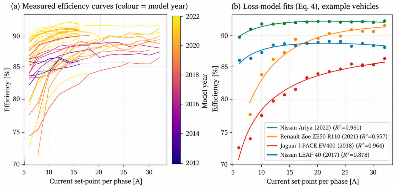
Equation (4) was fitted independently to the valid three-phase efficiency measurements of each vehicle using trust-region-reflective nonlinear least squares implemented through scipy.optimize.curve_fit [21]. Non-negativity constraints were imposed on all three coefficients to preserve their physical interpretation. For a vehicle with $n$ valid operating points, the fitted parameters were obtained from

$$\left(\widehat{a},\widehat{b},\widehat{c}\right)=\mathrm{a}\mathrm{r}\mathrm{g}\hspace{0.17em}\mathrm{m}\mathrm{i}\mathrm{n}\hspace{0.17em}\mathrm{a},\mathrm{b},\mathrm{c}\ge 0{\displaystyle \sum _{i=1}^n}{\left[{\eta }_i−\eta ,\left(I_i;a,b,c\right)\right]}^2.$$

(6)

The optimisation was initialised using

$$(a,b,c)=\left(0.5, 0.05, {10}^{-4}\right).$$

Only experimentally valid current set-points were included in the objective function. Vehicles with fewer than four valid efficiency observations were excluded from parameter fitting because the available information was considered insufficient for stable estimation of three constrained coefficients. Converged boundary estimates (e.g., b = 0) were treated as unresolved components, not confirmed zero losses.

• Efficiency-optimal operating point

Differentiating Equation (4) with respect to current gives

$${\displaystyle \frac{\mathrm{d}\eta }{\mathrm{d}I}}={\displaystyle \frac{a}{I^2}}-c.$$

Setting the derivative equal to zero produces the interior efficiency-optimal current:

$$I^{\ast }=\sqrt{{\displaystyle \frac{a}{c}}}.$$

(7)

At $I^{\ast }$, the fixed-loss and ohmic-loss contributions are equal. Substitution into Equation (4) yields the corresponding model-predicted peak efficiency:

$${\eta }^{\ast }=\eta ,\left(I^{\ast }\right)=1-b-2\sqrt{ac}.$$

(8)

The coefficient $a$ therefore governs the depth of the low-current efficiency penalty, whereas $b$ and the geometric mean $\sqrt{ac}$ jointly determine the attainable efficiency ceiling. Where $I^{\ast }$ exceeded the largest experimentally supported current, the vehicle was interpreted as exhibiting a monotonically increasing efficiency curve over the measured range, and the observed optimum occurred at the maximum available current set-point.

• Model-fit evaluation

Goodness of fit was evaluated using the coefficient of determination,

$$R^2=1-{\displaystyle \frac{{\displaystyle {\sum }_{i=1}^n}{\left({\eta }_i−{\widehat{\eta }}_i\right)}^2}{{\displaystyle {\sum }_{i=1}^n}{\left({\eta }_i−\overline{\eta }\right)}^2}},$$

(9)

and the root mean square error,

$$\mathrm{R}\mathrm{M}\mathrm{S}\mathrm{E}=\sqrt{{\displaystyle \frac{1}{n}}{\displaystyle \sum _{i=1}^n}{\left({\eta }_i−{\widehat{\eta }}_i\right)}^2}.$$

(10)

For nearly flat efficiency curves, the denominator of Equation (9) becomes small, meaning that modest absolute residuals can produce comparatively low $R^2$ values. RMSE was therefore treated as the primary measure of absolute fit quality, while $R^2$ was retained as a complementary measure of explained variation.

• Feature construction

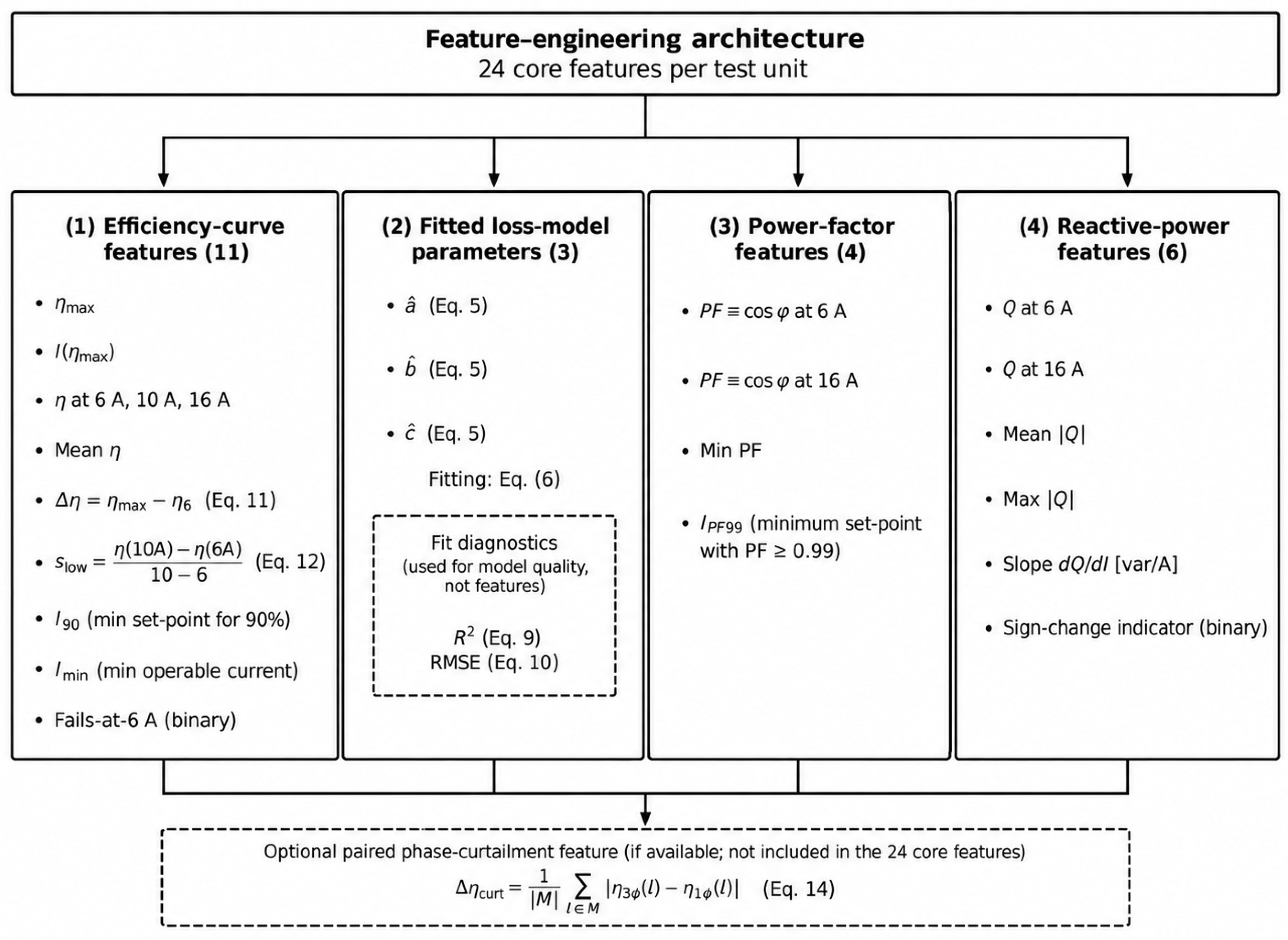
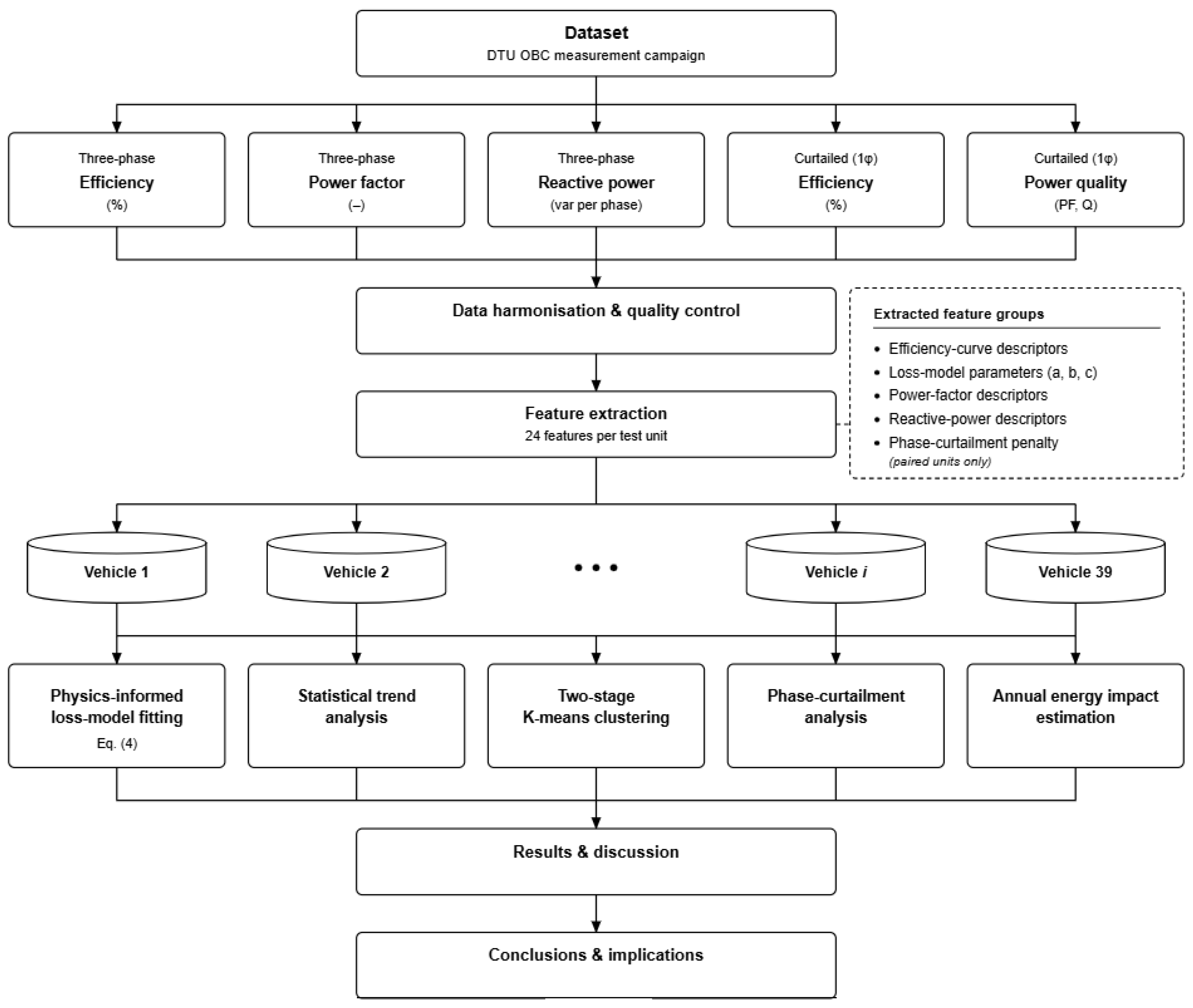
A total of 24 analytical features were extracted for each test unit. These features were organised into three principal blocks: efficiency curve descriptors, physics-informed loss coefficients, and grid-side power quality descriptors. The $R^2$ and RMSE values were retained as model-fit diagnostics but were not counted among the 24 characterisation features. Figure 3 summarises the complete feature-engineering architecture.

• Efficiency curve descriptors

Eleven features were extracted from each valid three-phase efficiency curve: peak measured efficiency, ${\eta }_{\mathrm{m}\mathrm{a}\mathrm{x}}$; the corresponding current set-point, $I\left({\eta }_{\mathrm{m}\mathrm{a}\mathrm{x}}\right)$; efficiencies at 6 A, 10 A, and 16 A; mean efficiency over all valid set-points; the low-current part-load penalty; the low-current efficiency slope; the minimum current required to reach 90% efficiency, $I_{90}$; the minimum operable current, $I_{\mathrm{m}\mathrm{i}\mathrm{n}}$; and the binary fails-at-6 A indicator. The low-current part-load penalty was defined as

$$\Delta \eta ={\eta }_{\mathrm{m}\mathrm{a}\mathrm{x}}-{\eta }_6.$$

(11)

For vehicles with valid observations at both 6 A and 10 A, the low-current slope was calculated as

$$s_{\mathrm{l}\mathrm{o}\mathrm{w}}={\displaystyle \frac{\eta (10 \mathrm{A})-\eta (6 \mathrm{A})}{10 \mathrm{A}-6 \mathrm{A}}},$$

(12)

and was reported in percentage points per ampere. The threshold feature $I_{90}$ was defined as the smallest measured current set-point at which conversion efficiency reached or exceeded 90%.

• Physics-informed loss descriptors

The fitted coefficients $\widehat{a}$, $\widehat{b}$, and $\widehat{c}$ constituted three additional features. These parameters provide more physically interpretable information than curve-shape descriptors alone because they separately represent low-current fixed-loss behaviour, proportional converter losses, and high-current ohmic effects. The coefficient of determination and RMSE were retained as diagnostic quantities for evaluating the numerical adequacy of each vehicle-level fit. They were not included in the primary count of 24 behavioural features because they describe model-fit quality rather than the underlying electrical behaviour of the OBC.

• Power-factor and reactive-power descriptors

Power quality features were derived from the measured power factor, denoted by $\lambda$, and the measured per-phase reactive power, denoted by $Q$. Their relationships to active and apparent power are

$$\lambda (I)={\displaystyle \frac{P_{\mathrm{A}\mathrm{C}}(I)}{S_{\mathrm{A}\mathrm{C}}(I)}},Q(I)=P_{\mathrm{A}\mathrm{C}}(I)\mathrm{t}\mathrm{a}\mathrm{n} \varphi (I),$$

(13)

where $S_{\mathrm{A}\mathrm{C}}$ is the apparent power. Four power-factor features were extracted: power factor at 6 A, power factor at 16 A, minimum measured power factor, and the smallest current set-point at which $\lambda \ge 0.99$, denoted by $I_{\mathrm{P}\mathrm{F}99}$. Six reactive-power features were extracted: reactive power at 6 A, reactive power at 16 A, mean absolute reactive power, maximum absolute reactive power, the ordinary-least-squares slope of $Q\left(I\right)$ in var/A, and a binary indicator identifying a capacitive-to-inductive or inductive-to-capacitive sign transition. Together, the 11 efficiency curve descriptors, three loss coefficients, four power-factor features, and six reactive-power features produced the 24-dimensional analytical representation.

• Same-current phase-configuration descriptor

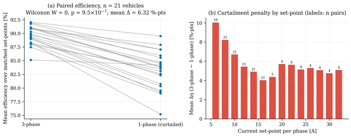
For the 21 vehicles with matched three-phase and curtailed single-phase efficiency measurements, a same-current configuration difference was calculated over the common set of valid per-phase current set-points:

$$\Delta {\eta }_{\mathrm{c}\mathrm{u}\mathrm{r}\mathrm{t}}={\displaystyle \frac{1}{\mid \mathcal{M}\mid }}\sum _{I\in \mathcal{M}}\left[{\eta }_{3\varphi }\left(I\right)-{\eta }_{1\varphi }\left(I\right)\right],$$

(14)

where M denotes the set of per-phase current values measured under both configurations. This within-vehicle comparison controls for vehicle identity and current set-point, but it does not hold total charging power constant: at the same per-phase current, single-phase operation transfers approximately one third of the power of three-phase operation. The statistic is therefore interpreted as a combined phase-configuration and total-throughput difference, not as a causal phase-only effect.

3.2. Statistical Analyses and Same-Current Configuration Comparison

• Model–year technology trends

Technology trends were examined by relating each vehicle-level response $y_i$ to model year $x_i$. The ordinary-least-squares slope was calculated as

$$\widehat{\beta }={\displaystyle \frac{{\displaystyle {\sum }_{i=1}^n}\left(x_i-\overline{x}\right)\left(y_i−\overline{y}\right)}{{\displaystyle {\sum }_{i=1}^n}{\left(x_i−\overline{x}\right)}^2}}.$$

(15)

Uncertainty was quantified using a 10,000-replicate nonparametric case-resampling bootstrap. Vehicles were sampled with replacement, Equation (15) was recomputed for each bootstrap replicate, and the percentile-based 95% confidence interval was defined as

$${\mathrm{C}\mathrm{I}}_{95\%}\left(\beta \right)=\left[{\beta }_{0.025}^{\ast }, {\beta }_{0.975}^{\ast }\right],$$

(16)

where ${\beta }_q^{\mathrm{*}}$ denotes the $q$-quantile of the bootstrap slope distribution. Monotonic association was evaluated using Spearman’s rank correlation:

$${\rho }_{\mathrm{s}}=\mathrm{c}\mathrm{o}\mathrm{r}\mathrm{r}\left[\mathrm{r}\mathrm{a}\mathrm{n}\mathrm{k}\left(x\right),\mathrm{r}\mathrm{a}\mathrm{n}\mathrm{k}\left(y\right)\right].$$

(17)

This formulation is appropriate in the presence of tied ranks and where the relationship is monotonic but not necessarily linear.

• Same-current paired configuration analysis

For vehicle $i$, the paired efficiency difference was defined as

$${\Delta }_i={\overline{\eta }}_{3\varphi ,i}-{\overline{\eta }}_{1\varphi ,i}.$$

The primary inferential procedure was the Wilcoxon signed-rank test. Its test statistic was calculated from the ranked absolute paired differences as

W = min(W⁺, W⁻), W⁺ = Σ(Δ_i > 0) R_i, W⁻ = Σ(Δ_i < 0) R_i.

(18)

where $R_i$ is the rank assigned to $\mid {\Delta }_i\mid$. A paired-samples $t$-test was additionally reported as a parametric sensitivity analysis. The standardised paired effect size was quantified using Cohen’s $d_z$:

$$d_z={\displaystyle \frac{\overline{\Delta }}{s_{\Delta }}},$$

(19)

where $\overline{\Delta }$ and $s_{\Delta }$ are the mean and standard deviation of the paired differences. The matched-pairs rank-biserial correlation was calculated as

rᵣᵦ = (W⁺ − W⁻)/(W⁺ + W⁻).

(20)

• Across-group comparisons

Differences among the reference behavioural groups were evaluated using the Kruskal–Wallis test:

$$H={\displaystyle \frac{12}{N(N+1)}}{\displaystyle \sum _{j=1}^g}{n}_j{\overline{R}}_j^{ 2}-3(N+1),$$

(21)

where N is the total number of observations, g is the number of reference groups, n_j is the size of group j, and R_j is its mean rank. Tie corrections were applied computationally. Two-sided p-values were used throughout. Because the finer partition is exploratory and some groups are small, these tests are treated as descriptive screening rather than as proof of a population-level taxonomy.

3.3. Exploratory Clustering, Feature Selection, and Stability Analysis

• Clustering variables and preprocessing

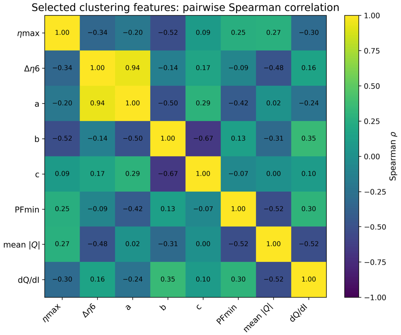
The 24 variables were retained for descriptive characterisation, but they were not all entered into K-means. The primary clustering set was reduced to eight variables chosen to represent complementary electrical dimensions while excluding identifiers, sparse threshold variables, binary indicators, direct duplicate-current measures, and an exact algebraic redundancy: peak efficiency (ηmax), the 6 A part-load difference (Δη6 = ηmax − η6), fitted coefficients a, b, and c, minimum power factor (PFmin), log10(mean |Q|), and reactive-power slope dQ/dI. The η6 descriptor was excluded because η6 = ηmax − Δη6, so retaining ηmax, η6, and Δη6 would exactly duplicate one degree of information. The logarithmic transformation was applied to mean absolute reactive power because its magnitude spans approximately two orders. Each selected variable was standardised before clustering:

$$z_{ij}={\displaystyle \frac{x_{ij}-{\mu }_j}{{\sigma }_j}},$$

(22)

where μj and σj are the sample mean and sample standard deviation of feature j. Missing power quality descriptors affected three of the 36 efficiency-characterised test units and were median-imputed after feature assembly. The remaining selected variables were available from the measured or fitted data. The Spearman screening showed that Δη6 and a remained strongly associated (ρ = 0.94); therefore, reduced-feature reruns excluding either member of this pair were included as sensitivity checks rather than claiming complete statistical independence among the eight variables. 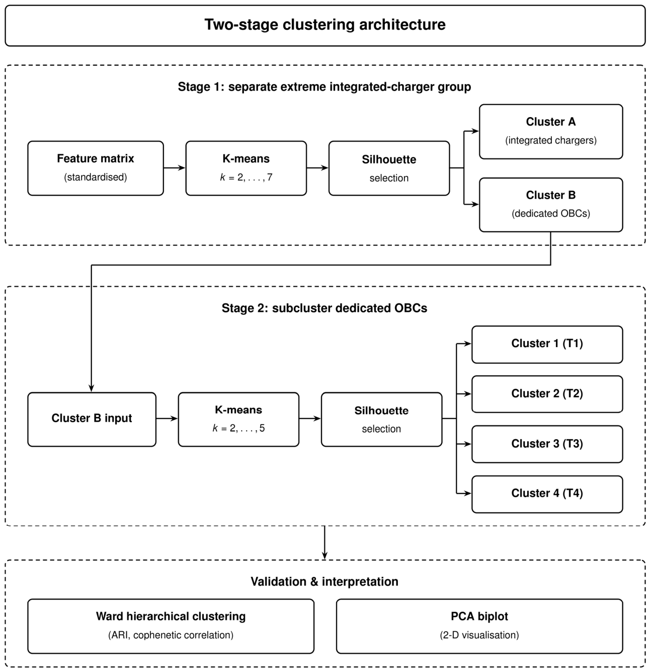Figure 4 illustrates the exploratory two-stage clustering and stability-analysis workflow.

• Stage 1 partition

Stage 1 applied K-means clustering with 50 independent initialisations and a fixed random seed of 42. For a candidate partition containing $k$ clusters, the method minimised the within-cluster sum of squares:

$$J\left(C_1,\dots ,C_k\right)={\displaystyle \sum _{r=1}^k}\sum _{i\in C_r}{\parallel {\mathbf{z}}_i-{\mathit{\mu }}_r\parallel }_2^2,$$

(23)

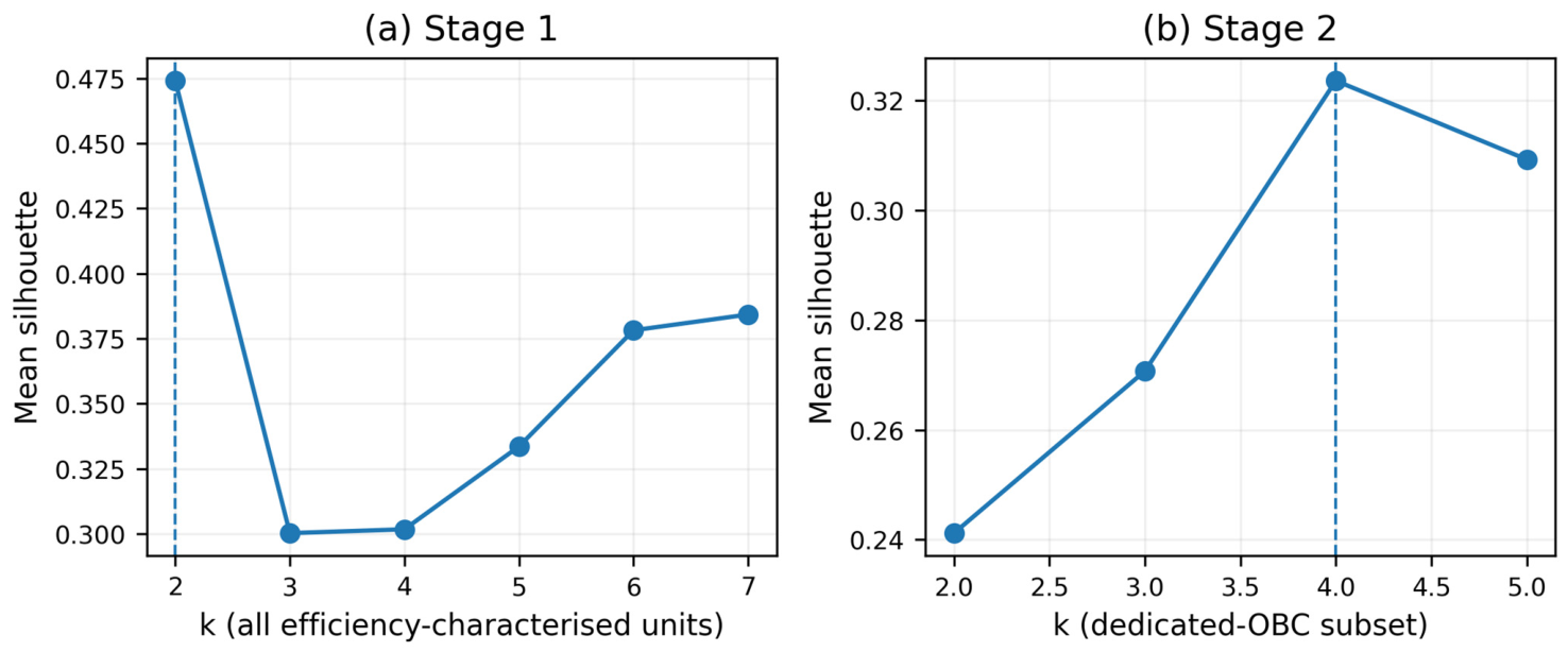
where ${\mathbf{z}}_i$ is the standardised feature vector of vehicle $i,$and ${\mathit{\mu }}_r$ is the centroid of cluster $C_r$. Candidate solutions were evaluated for $k=2,\dots ,7$. The preferred number of clusters was selected using the mean silhouette coefficient [22]. For observation $i$,

$$s(i)={\displaystyle \frac{b\left(i\right)-a\left(i\right)}{\mathrm{m}\mathrm{a}\mathrm{x}\left\{a\right(i),b(i\left)\right\}}},$$

(24)

where $a\left(i\right)$ is the mean distance between observation $i$ and the other members of its assigned cluster, whereas $b\left(i\right)$ is the smallest mean distance between $i$ and any alternative cluster.

• Ward method comparison

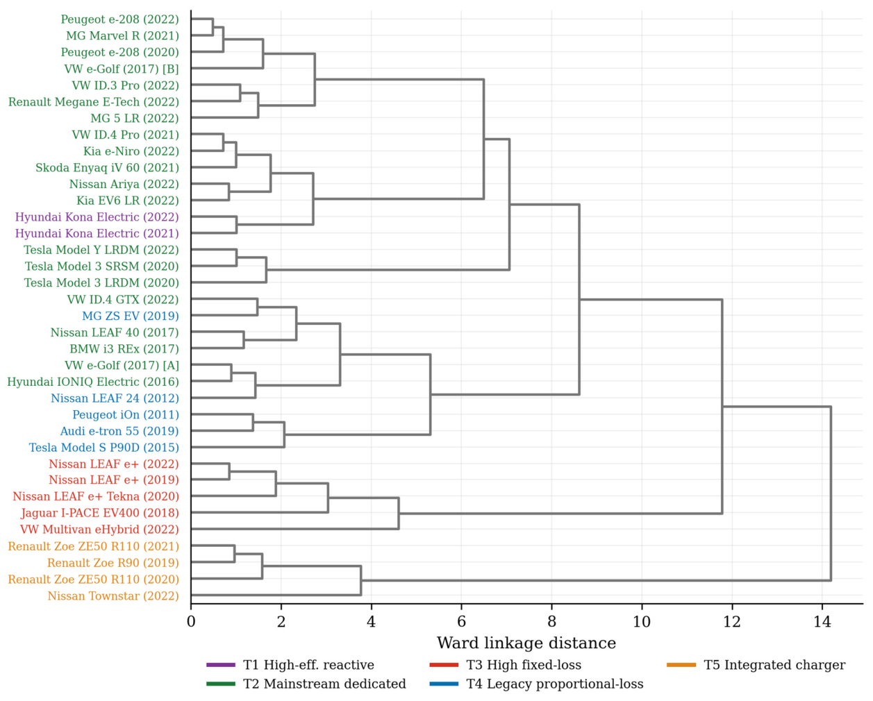
The Stage 1 partition was independently evaluated using agglomerative hierarchical clustering with Ward linkage. At each step, the pair of clusters producing the smallest increase in total within-cluster variance was merged according to

$$d_{\mathrm{W}}\left(C_p,C_q\right)={\displaystyle \frac{\mid C_p\mid \mid C_q\mid }{\mid C_p\mid +\mid C_q\mid }}{\parallel {\mathit{\mu }}_p-{\mathit{\mu }}_q\parallel }_2^2.$$

(25)

Dendrogram fidelity was quantified using the cophenetic correlation coefficient:

$$r_{\mathrm{c}\mathrm{o}\mathrm{p}\mathrm{h}}=\mathrm{c}\mathrm{o}\mathrm{r}\mathrm{r}\left(d_{ij},t_{ij}\right),$$

(26)

where $d_{ij}$ is the original pairwise distance between observations $i$ and $j$, and $t_{ij}$ is the corresponding cophenetic distance in the hierarchical tree. Agreement between the K-means and Ward partitions was quantified using the adjusted Rand index [23]:

$$\mathrm{A}\mathrm{R}\mathrm{I}={\displaystyle \frac{\mathrm{R}\mathrm{I}-\mathbb{E}\left[\mathrm{R}\mathrm{I}\right]}{\mathrm{m}\mathrm{a}\mathrm{x}\left(\mathrm{R}\mathrm{I}\right)-\mathbb{E}\left[\mathrm{R}\mathrm{I}\right]}}.$$

(27)

An ARI of 1 indicates identical partitions, whereas a value near 0 indicates agreement no greater than expected under random labelling.

• Exploratory Stage 2 partition

The two-stage strategy was not preregistered or specified independently of the data. It was adopted after the silhouette-optimal Stage 1 solution (k = 2) isolated four electrically extreme motor-winding-integrated chargers from the remaining 32 units. Stage 2 then re-standardised and reclustered the 32-unit dedicated OBC subset for k = 2, …, 5. The resulting four subgroups, together with the Stage 1 minority group, define the five-group reference partition used for descriptive comparisons. Because this is a data-informed second step and Stage 2 separation is only moderate, the groups are not presented as universal OBC behavioural groups.

Stability was evaluated in four ways. First, Ward hierarchical clustering was compared with K-means using the adjusted Rand index (ARI) and cophenetic correlation. Second, 1000 vehicle-level bootstrap resamples were fitted with the same two-stage pipeline; labels were optimally aligned to the reference partition and ARI, assignment accuracy, and groupwise Jaccard overlap were recorded. Third, each test unit was removed in turn, and the full pipeline was rerun, with both fixed-k agreement and silhouette-selected k recorded. Fourth, sensitivity analyses removed the two-unit high-efficiency/reactive group, removed the integrated-charger group, and repeated clustering after excluding highly correlated efficiency/loss descriptors. These analyses test the dependence of the finer partition on individual vehicles, small groups, and feature choice.

• Principal component visualisation

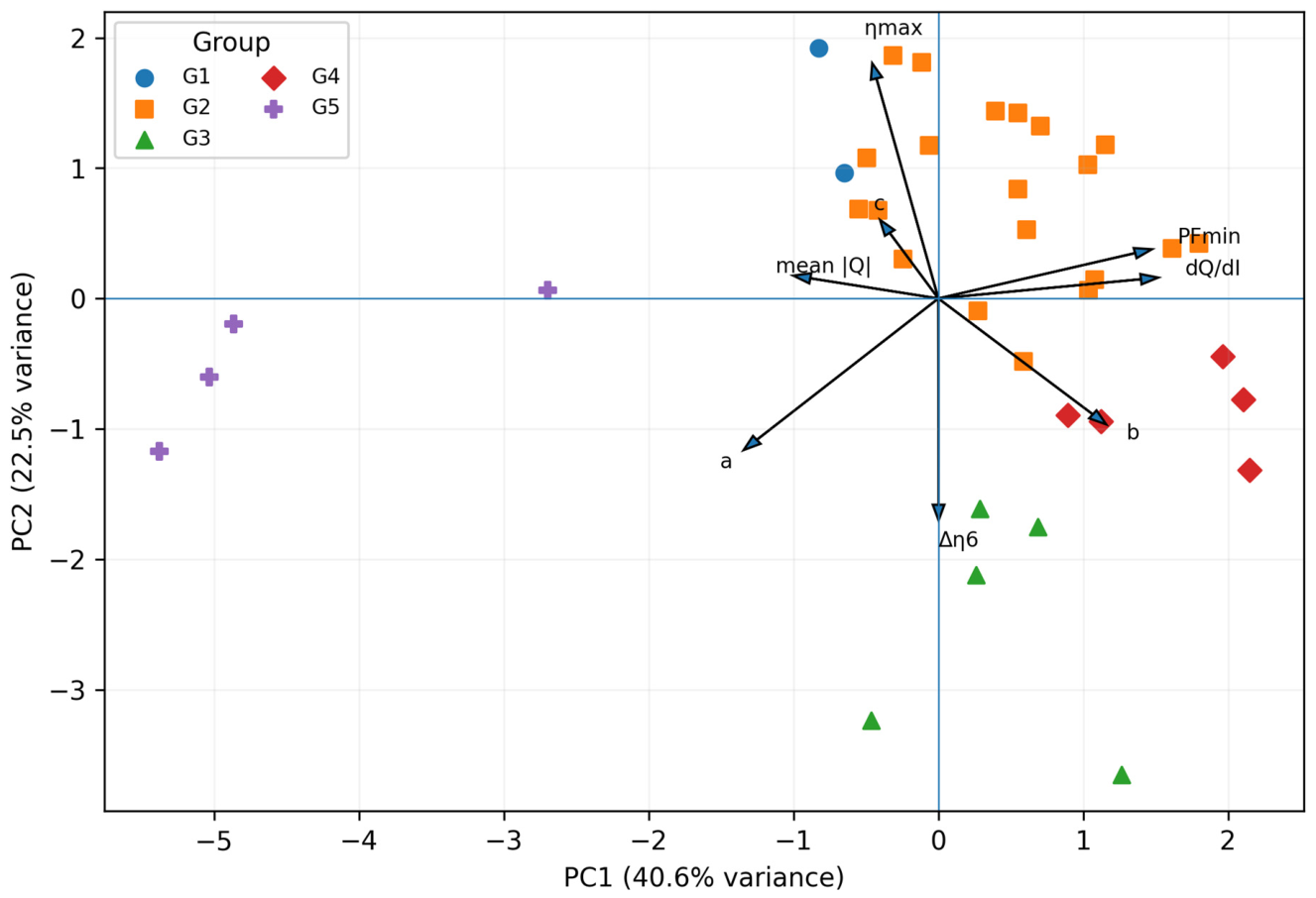
Principal component analysis was used exclusively for visualisation and did not determine cluster membership. For the standardised feature matrix $\mathbf{Z}$, the sample covariance matrix was calculated as

$$\mathbf{S}={\displaystyle \frac{{\mathbf{Z}}^{\mathsf{T}}\mathbf{Z}}{n-1}}.$$

The principal axes were obtained from

$$\mathbf{S}{\mathbf{v}}_k={\lambda }_k{\mathbf{v}}_k,$$

(28)

where ${\lambda }_k$ and ${\mathbf{v}}_k$ are the $k$-th eigenvalue and eigenvector. The first two eigenvectors defined the biplot axes, while the corresponding feature coefficients were displayed as loading vectors.

3.4. Annual Energy Scenario and Sensitivity Analysis Approach

The measured current-dependent efficiencies were translated into annual energy using a transparent reference scenario. The baseline case assumes 2500 kWh/year of DC energy delivered to the battery:

$$D=2500 \mathrm{k}\mathrm{W}\mathrm{h} \mathrm{y}\mathrm{e}\mathrm{a}{\mathrm{r}}^{-1}$$

This reference corresponds to approximately 13,900 km/year at 0.18 kWh/km. It is not intended to represent every user. For battery-delivered annual energy D and operating efficiency η, the required grid-side AC energy is

$$E_{\mathrm{A}\mathrm{C}}={\displaystyle \frac{D}{\eta }}.$$

(29)

The corresponding annual conversion loss is

$$L(\eta )=E_{\mathrm{A}\mathrm{C}}-D=D\left({\displaystyle \frac{1}{\eta }}−1\right).$$

(30)

Two bounding policies define a transparent upper-contrast reference. Under Pbest, all delivered energy is charged at the vehicle’s most efficient measured current set-point (ηmax). Under Pmin, all delivered energy is charged at the minimum supported current, with efficiency denoted ηmin. The resulting difference is

$$\Delta L_{\mathrm{d}\mathrm{m}}=L({\eta }_{\mathrm{l}\mathrm{o}\mathrm{w}})-L({\eta }_{\mathrm{m}\mathrm{a}\mathrm{x}})=D\left({\displaystyle \frac{1}{{\eta }_{\mathrm{l}\mathrm{o}\mathrm{w}}}}−{\displaystyle \frac{1}{{\eta }_{\mathrm{m}\mathrm{a}\mathrm{x}}}}\right).$$

(31)

For the paired three-phase and curtailed single-phase measurements, the analogous annualised same-current configuration contrast is

$$\Delta L_{\mathrm{c}\mathrm{u}\mathrm{r}\mathrm{t}}=D\left({\displaystyle \frac{1}{{\overline{\eta }}_{1\varphi }}}−{\displaystyle \frac{1}{{\overline{\eta }}_{3\varphi }}}\right).$$

(32)

These quantities are controlled scenario contrasts, not predictions of an individual user’s realised annual loss. Sensitivity analysis therefore varies annual battery-delivered energy (1500, 2500, and 4000 kWh/year) and the fraction of energy delivered at the minimum-current operating point (20%, 50%, 80%, and 100%). An additional residential/public mix example varies the share of annual energy assigned to home AC charging and the fraction of home energy delivered at minimum current; the remaining energy is treated as best-set-point AC charging for the purpose of isolating OBC conversion effects. SOC-specific or time-resolved smart-charging profiles are not simulated because the source dataset does not contain the required SOC trajectories, timestamps, or charging session load profiles.

3.5. Computational Reproducibility

The feature-level analyses were conducted in Python 3 using pandas, NumPy 1.2, SciPy 1.18.0, scikit-learn 1.9.1, and Matplotlib 3.11.2 [21,24]. Random seeds were fixed where stochastic algorithms were used. The supplementary reproducibility package contains the analysis-ready vehicle-feature table, the clustering/stability/scenario script, the analysis-label identifier map, and a README describing execution. The package reproduces the clustering, stability, group-summary, and annual sensitivity results from the reported feature inputs. The underlying raw measurements remain publicly available through DTU Data [20].

4. Results and Discussion

This section reports the measured OBC characteristics, loss-model results, power quality behaviour, model–year trends, exploratory grouping and stability analyses, the same-current three-phase versus curtailed single-phase comparison, and annual energy sensitivity. Results inherited directly from the source measurements are distinguished from quantities generated by the present reanalysis.

4.1. Results

4.1.1. Measured OBC Efficiency Landscape

Of the 39 test units, three (the Volvo XC40 Recharge and two Polestar 2 variants) contain power quality measurements but no conversion-efficiency observations, leaving 36 units for efficiency curve and loss-model analyses. Figure 5 displays the source efficiency measurements [20]. Their general rise with charging current and the inability of several integrated-charger vehicles to sustain 6 A are properties of the published experimental dataset rather than new measurements produced by this study; the new analysis begins with their loss-model parameterisation and subsequent feature-level comparisons.

4.1.2. Physics-Informed Loss-Model Performance

The physics-informed model defined in Equation (4) provided a strong representation of the vehicle-level efficiency curves. vehicle-level efficiency and fitted-loss descriptors are provided in the Supplementary Materials. Across the 36 fitted test units, the median coefficient of determination was $R^2=0.968$, while the median RMSE was 0.22 percentage points. A total of 31 of the 36 fitted vehicles achieved $R^2>0.89$. The lowest $R^2$ values were obtained for the Peugeot iOn ($R^2=0.14$), Audi e-tron 55 ($R^2=0.59$), Nissan LEAF 40 ($R^2=0.88$), and MG ZS EV ($R^2=0.89$). These vehicles exhibit comparatively flat measured efficiency curves, resulting in a small denominator in Equation (9). Their RMSE values remained between 0.27 and 0.84 percentage points, confirming that the absolute fitting errors were small despite the reduced explained-variance values. The analytic optimum derived in Equations (7) and (8) also agreed closely with the measured operating behaviour. Of the 30 vehicles with a non-degenerate ohmic-loss coefficient, $\widehat{c}>0$, 18 had a predicted optimal current

$$I^{\mathrm{*}}=\sqrt{{\displaystyle \frac{\widehat{a}}{\widehat{c}}}},$$

above the maximum experimentally supported current. This result is consistent with their monotonically increasing measured efficiency curves. For the 12 vehicles with an interior optimum, the model-predicted current agreed with the observed optimum to a median absolute difference of 1.8 A, approximately one experimental current increment. The model-predicted peak efficiency,

$${\eta }^{\ast }=1-\widehat{b}-2\sqrt{\widehat{a}\widehat{c}},$$

differed from the observed maximum by a median of only 0.15 percentage points. The fitted coefficients also exhibited clear physical differentiation. The fixed-loss coefficient $\widehat{a}$ had a fleet-wide mean of 0.70 A with a standard deviation of 0.48 A. Its mean value was 1.68 A for the motor-winding-integrated charger group, approximately 2.4 times the corresponding mean of 0.57 A for the remainder of the fleet. The proportional coefficient $\widehat{b}$ exhibited the opposite pattern, averaging 0.006 for the integrated chargers and 0.054 for the other vehicles. This contrast provides a direct quantitative signature of the different OBC conversion architectures. The ohmic coefficient $\widehat{c}$ remained comparatively small, with a mean of approximately $1.3\times {10}^{-3}{\mathrm{A}}^{-1}$. Figure 6a presents all measured three-phase efficiency curves coloured by model year, while Figure 6b shows representative measured and fitted curves spanning the identified OBC behavioural groups. Peak efficiency across the corpus averaged 89.6%, with a standard deviation of 2.5% and a range of 82.9–93.1%. Efficiency at 6 A averaged 84.3%, with a standard deviation of 5.4% and a range of 69.3–90.6%. The mean part-load penalty was 5.1 percentage points and reached a maximum of 14.7 percentage points for the Jaguar I-PACE.

4.1.3. Power-Factor and Reactive-Power Behaviour

Figure 7 presents the measured grid-side power quality behaviour. Most dedicated OBCs operated with a power factor above 0.97 over the supported current range and reached a power factor of at least 0.99 between approximately 10 and 14 A. Two vehicle groups departed substantially from this general behaviour. The Hyundai Kona test units combined high conversion efficiency with a pronounced reactive-power response, reaching approximately 1.8 kvar at current set-points of 10–12 A and minimum power factors of approximately 0.91. The motor-winding-integrated chargers—including the Renault Zoe R90, Renault Zoe ZE50 variants, and Nissan Townstar—exhibited the most severe low-current power quality behaviour. Their minimum power factors ranged from approximately 0.54 to 0.87, while their low-current reactive-power magnitudes reached approximately 2–5 kvar. These vehicles also displayed steep negative reactive-power slopes and, in several cases, capacitive-to-inductive sign transitions. By contrast, the Tesla Model 3 and Model Y test units maintained absolute reactive-power magnitudes below approximately 45 var throughout the measured range, indicating grid-side operation close to unity power factor.

4.1.4. Technology Trends in OBC Performance

Table 3. Technology-trend regressions of OBC characteristics against model year, 2011–2022.

Feature	n	OLS Slope/Year	95% CI Low	95% CI High	Pearson r	p (OLS)	Spearman ρ	p (Spearman)
Peak efficiency (%)	36	0.533	0.324	0.774	0.618	<1 × 10−4	0.648	<1 × 10−4
Efficiency at 6 A (%)	32	0.450	−0.034	1.198	0.248	0.171	0.506	0.003
Mean efficiency (%)	36	0.514	0.234	0.858	0.472	0.004	0.599	1 × 10−4
Fixed-loss coefficient a (A)	36	0.022	−0.036	0.058	0.130	0.450	−0.027	0.875
Power factor at 6 A	32	0.003	−0.0001	0.0048	0.407	0.021	0.412	0.019
Mean |Q| (var)	37	18.422	−46.887	64.914	0.089	0.603	0.158	0.351

reports the formal regressions of the selected OBC features against vehicle model year. Peak conversion efficiency increased by 0.5333 percentage points per model year, with a 95% bootstrap confidence interval of 0.3242–0.7736 percentage points per year. The relationship was supported by both the Pearson correlation, $r=0.6183$, and the Spearman rank correlation, $\rho =0.6484$. Mean OBC efficiency increased by 0.5136 percentage points per model year. Efficiency at 6 A also exhibited a positive rank-based association with model year, although the bootstrap confidence interval for the ordinary-least-squares slope crossed zero. This indicates that low-current improvement was heterogeneous across the fleet, with several recent vehicles continuing to exhibit weak part-load performance. The fixed-loss coefficient $\widehat{a}$ showed no meaningful temporal trend. Its Spearman correlation with model year was $\rho =-0.0273$, with $p=0.8746$. This finding indicates that improvements in the OBC efficiency ceiling were not accompanied by a systematic reduction in the fixed-loss component that dominates low-current charging. Power factor at 6 A improved modestly with model year, whereas mean absolute reactive power did not exhibit a statistically meaningful trend.

Figure 8 illustrates the model–year relationships for peak efficiency and efficiency at the minimum operable current.

4.1.5. Feature-Correlation Structure

Figure 9 presents the Spearman correlation structure of the eight-variable clustering set. Peak efficiency is negatively associated with the proportional-loss coefficient, while the 6 A part-load difference Δη6 is strongly associated with the fitted fixed-loss coefficient a (ρ = 0.94). Minimum power factor is negatively associated with mean absolute reactive power. These relationships confirm that the selected variables are physically interpretable but not statistically orthogonal; cluster sensitivity to feature removal is therefore reported below.

4.1.6. Exploratory OBC Behavioural Groups and Stability

With the eight-variable input, Stage 1 selected k = 2, with a mean silhouette coefficient of 0.474. The minority group comprised the Renault Zoe R90, both Renault Zoe ZE50 test units, and the Nissan Townstar; the remaining 32 units formed the dedicated OBC subset. Ward clustering reproduced this Stage 1 split exactly (ARI = 1.00) with a cophenetic correlation of 0.81. The stability of this top-level separation supports treating the integrated-charger group as a strong within-dataset structure.

After re-standardisation of the 32 dedicated OBCs, Stage 2 selected k = 4, but the maximum mean silhouette coefficient was only 0.324, indicating appreciable overlap among the finer groups. Ward clustering of the dedicated subset showed substantial but not exact agreement with the four-group K-means partition (ARI = 0.869; cophenetic correlation = 0.665). Accordingly, the finer groups are treated as an exploratory within-dataset reference rather than as externally validated OBC classes.

Resampling confirmed the distinction between the robust top-level split and the less stable finer partition. In 36 leave-one-out reruns, Stage 1 selected k = 2 in every case; Stage 2 selected k = 4 in 30 cases, k = 5 in five cases, and k = 3 in one case. For the fixed-k pipeline, the median leave-one-out ARI was 1.00, but the minimum was 0.424 when influential individual vehicles were omitted. Across 1000 bootstrap resamples, the median ARI relative to the five-group reference partition was 0.429 (95% empirical interval 0.152–0.968), and the median aligned assignment accuracy was 0.667. Only 11.7% of resamples achieved ARI >= 0.80. The integrated-charger group (G5) had the highest bootstrap Jaccard stability (median 1.00; mean 0.956), whereas the finer dedicated OBC groups were substantially less stable. Removing the two-unit G1 group changed the preferred Stage 2 solution, further demonstrating small-group sensitivity.

Feature sensitivity gave the same message. Eliminating the exact redundant η6 descriptor retained the five-group reference memberships while increasing the Stage 1 silhouette coefficient. Residual redundancy remained important: removing Δη6 preserved the Stage 1 k = 2 split but changed the preferred Stage 2 solution from k = 4 to k = 5 and reduced agreement with the reference partition to ARI = 0.497. Removing the retained Stage 2 k = 4 produced ARI = 0.968 relative to the reference partition. These results reinforce that the top-level integrated-charger separation is more stable than the finer dedicated OBC partition. The five groups are therefore retained only as a convenient descriptive reference for the measured units and are not claimed to be population-level OBC classes. Figure 10 illustrates the silhouett-based cluster-number selection using the eight-variable feature set.

Table 4. Efficiency and fitted-loss characteristics of the five dataset-derived reference groups.

Group	n	ηmax (%)	η6 (%)	Δη6 (pp)	a (A)	b (-)	c (A−1)
G1	2	92.34	89.12	3.22	0.425	0.028	0.002
G2	20	90.59	86.78	3.81	0.501	0.039	0.002
G3	5	86.95	74.01	12.94	1.156	0.067	0.001
G4	5	86.25	83.02	3.23	0.336	0.115	0.001
G5	4	90.57	c	-	1.683	0.006	0.001

and

Table 5. Power quality and contextual characteristics of the five dataset-derived reference groups.

Group	n	PFmin	Mean |Q| (Var)	dQ/dI (Var/A)	Mean Year	Δηcfg (pp)
G1	2	0.917	1446	−45.8	2021.5	4.07
G2	20	0.986	421	0.3	2020.2	7.04
G3	5	0.971	238	−1.5	2020.2	-
G4	5	0.959	551	17.7	2015.2	0.93
G5	4	0.648	2000	−244.6	2020.5	6.02

summarise the five dataset-derived reference groups. G1 contains the two high-efficiency Hyundai Kona units with pronounced reactive-power behaviour; G2 is the large mainstream dedicated OBC group; G3 contains units with severe low-current deterioration and large fixed-loss terms; G4 contains older, higher proportional-loss units; and G5 contains the four motor-winding-integrated chargers. These labels are descriptive shorthand for this dataset, not universal classes.

G2 represents the large mainstream dedicated OBC group, with a mean peak efficiency of approximately 90.6%, moderate fitted fixed losses, and near-unity minimum power factor. G1 has the highest mean peak efficiency but elevated reactive-power magnitude. G3 is distinguished by a mean 6 A part-load difference of approximately 12.9 percentage points and the largest fitted fixed-loss coefficient among the dedicated OBCs. G4 contains the oldest mean model year and the largest proportional-loss coefficient. G5 combines relatively high peak efficiency with weak low-current operation, reduced power factor, and the largest reactive-power magnitudes. Given the resampling results, these descriptions apply to the measured units and should not be extrapolated as stable population clusters. The two independently measured 2017 VW e-Golf units were both assigned to G2, providing an internal repeatability check for the descriptive grouping. Figure 11 presents the principal component biplot of the eight-variable standardised space. The first two principal components explain 63.2% of the total variance (40.6% and 22.5%, respectively). The loading vectors indicate the direction and relative contribution of each variable to the visual separation; PCA is used only for visualisation and does not determine group membership.

Figure 12 presents the Ward-linkage dendrogram for the 36 efficiency-characterised units using the eight-variable set. The top-level split isolates the integrated-charger group, consistent with the Stage 1 ARI of 1.00; the lower branches also illustrate the weaker separation among dedicated OBC groups.

4.1.7. Same-Current Three-Phase Versus Curtailed Single-Phase Comparison

Across the 21 vehicles with paired three-phase and curtailed single-phase measurements, the mean three-phase minus single-phase efficiency difference at matched per-phase current set-points was 6.32 percentage points (SD 2.77; bootstrap 95% CI 5.18–7.49). Every paired vehicle had lower measured efficiency in curtailed single-phase operation. The Wilcoxon signed-rank test gave p = 9.5 × 10⁻⁷, the paired-samples test gave t = 10.47 with p = 1.4 × 10⁻⁹, Cohen’s dz = 2.29, and the matched-pairs rank-biserial correlation was 1.00.

Figure 13a compares the paired vehicle means, while Figure 13b shows the difference by per-phase current set-point. The difference exceeded approximately 9 percentage points at 6 A and declined towards approximately 2–4 percentage points above 20 A. This should not be interpreted as an isolated “phase penalty”: at the same per-phase current, curtailed single-phase operation transfers roughly one third of the total power of three-phase operation. The observed 6.32-percentage-point contrast therefore combines phase configuration with lower total power throughput and the associated amplification of fixed losses. The available dataset does not provide a systematic set of equal-total-power three-phase/single-phase pairs across the fleet, so a pure phase-count effect cannot be identified without additional experiments.

Table 6. Paired statistical evaluation of the same-current three-phase versus curtailed single-phase efficiency difference.

n	Mean Δ (pp)	SD (pp)	95% CI (pp)	Wilcoxon p	Cohen dz	Rank-Biserial
21	6.32	2.77	5.18–7.49	9.5 × 10−7	2.29	1.00

tabulates the paired statistical evaluation of the same-current three-phase versus curtailed single-phase efficiency difference.

4.1.8. Annual Energy Scenario and Sensitivity Analysis

Table 7. Annual OBC conversion losses and minimum-current versus best-set-point contrast by dataset-derived group for the 2500 kWh/year reference case.

Group	n	Lbest (kWh/y)	Lmin (kWh/y)	ΔL (kWh/y)	SD ΔL
G1	2	207.4	305.8	98.4	34.7
G2	20	260.3	383.1	122.9	53.0
G3	5	377.3	884.3	507.0	83.4
G4	5	399.6	512.5	112.9	90.5
G5	4	260.6	530.8	270.2	41.7

retains the 2500 kWh/year reference calculation as a transparent bounding comparison. Under the best measured set-point, mean annual OBC conversion losses are approximately 293 kWh/vehicle. Figure 14 illustrates the annual OBC scenario analysis. If every unit of annual battery-delivered energy were instead charged at the minimum supported current, the reference fleet-average additional conversion loss is approximately 190 kWh/year. This value is an extreme policy contrast, not an estimate of typical real-world charging behaviour. G3 and G5 show the largest group-average contrast, reflecting their weaker low-current efficiency.

Table 8. Sensitivity of the fleet-average additional conversion energy to annual battery-delivered energy and low-current charging fraction.

Annual DC Energy (kWh/y)	Energy at Minimum Current	Additional Grid Energy (kWh/y)
1500	20%	22.8
1500	50%	57.0
1500	80%	91.1
1500	100%	113.9
2500	20%	38.0
2500	50%	94.9
2500	80%	151.9
2500	100%	189.9
4000	20%	60.8
4000	50%	151.9
4000	80%	243.0
4000	100%	303.8

reports scenario sensitivity based on the 190 kWh/year fleet-average bounding contrast in Table 7. At 2500 kWh/year, moving 20%, 50%, and 80% of delivered energy from the best measured set-point to minimum-current operation scales the fleet-average additional energy to approximately 38, 95, and 152 kWh/year, respectively. At the 100% extreme, the corresponding values are approximately 114, 190, and 304 kWh/year for 1500, 2500, and 4000 kWh/year of battery-delivered energy. A 70% home–AC share with half of the home energy delivered at minimum current corresponds to an overall 35% low-current fraction and approximately 66 kWh/year of additional grid energy in the 2500 kWh/year reference case. These calculations isolate OBC conversion effects; they are not substitutes for SOC- and time-resolved charging simulations.

4.2. Discussion

4.2.1. OBC Efficiency and Part-Load Behaviour

The fitted loss model adds a physically interpretable layer to the source measurements. Ref. [20] already showed that current modulation can increase charging energy demand; the present decomposition attributes much of the vehicle-specific low-current deterioration to the fixed-loss term and shows that the fitted fixed-loss coefficient has no clear model–year trend. Peak efficiency therefore cannot, by itself, represent the energy implications of deep current modulation. This mechanism is qualitatively consistent with independent measurements showing reduced power–electronics efficiency at low power transfer [9], although Ref. [9] is not an external validation dataset for the present groups.

4.2.2. Power Quality and Topological Differences

The power quality results reinforce the need to distinguish conversion efficiency from grid-side electrical behaviour. Some high-efficiency units exhibit substantial reactive-power exchange, whereas other vehicles maintain near-unity power factor. The partial independence of the efficiency and power quality blocks supports their joint descriptive use, but the correlation analysis also shows that the selected clustering variables are not fully orthogonal.

4.2.3. Interpretation and Stability of Dataset-Derived Groups

The strongest grouping result is the Stage 1 separation of the four motor-winding-integrated chargers: it is reproduced exactly by Ward clustering and selected as k = 2 in every leave-one-out rerun. The finer partition of dedicated OBCs is materially less stable. Its Stage 2 silhouette coefficient is 0.324, bootstrap agreement with the five-group reference partition is modest, and removal of the two-unit G1 group changes the preferred Stage 2 solution. The five-group partition is therefore treated as a dataset-derived exploratory structure. It is useful for descriptive comparison, but its boundaries and group counts should not be assumed to persist in a larger or independent fleet.

4.2.4. Implications for Smart Charging and Aggregator Operation

The same-current three-phase versus curtailed single-phase comparison has practical relevance for schedulers, but its interpretation must be precise. The 6.32-percentage-point mean difference is observed at equal per-phase current, not equal total charging power; it therefore combines phase-count effects with the ordinary efficiency effect of operating the converter at lower total throughput. A controller that simultaneously reduces phase count and current may still incur a substantial conversion penalty, but the present data cannot separate the causal contribution of phase configuration from power level. Equal-total-power experiments or a source dataset with sufficiently overlapping three-phase and single-phase operating points are required for that identification.

4.2.5. External Validity, Limitations, and Future Work

The principal limitation is external validity. The physics-informed parameters, feature correlations, and behavioural groups are estimated from one DTU experimental campaign, and most models are represented by a single physical test unit. The resampling analyses quantify internal sensitivity but do not substitute for an independent validation set. The small G1 (n = 2) and G5 (n = 4) groups are especially unsuitable for population-level inference. Battery SOC, ambient and battery temperature, grid-voltage variation, ageing, and time-resolved charging trajectories are not fully resolved, so the annual energy analysis remains a controlled scenario study rather than a prediction of user behaviour. Future work should test the loss model and grouping procedure on independent EV fleets, repeated units of the same model, equal-total-power phase comparisons, and field charging profiles with SOC, temperature, voltage, tariffs, renewable availability, and network constraints. Closed-loop studies can then compare constant-efficiency scheduling with OBC-aware optimisation under realistic operating conditions.

5. Conclusions

This study reanalysed the open DTU OBC measurements using a physics-informed loss model, electrical feature construction, formal statistics, and stability-qualified exploratory clustering. The loss model reproduced vehicle-level efficiency curves with a median RMSE of 0.22 percentage points. Peak efficiency increased by approximately 0.53 percentage points per model year, but the fitted fixed-loss coefficient did not show a corresponding temporal improvement. The eight-variable clustering analysis identifies a robust top-level separation of four motor-winding-integrated chargers from the dedicated OBC sample, while the finer five-group reference partition has only moderate Stage 2 separation and substantial bootstrap sensitivity. It is therefore reported as a dataset-derived exploratory structure rather than as a general OBC taxonomy. Across 21 paired vehicles, three-phase efficiency exceeded curtailed single-phase efficiency by 6.32 percentage points on average at matched per-phase current, but this contrast also reflects the associated reduction in total power throughput and is not a phase-only causal estimate. The 2500 kWh/year annual energy calculation is likewise a bounding reference: continuous minimum-current operation gives an approximately 190 kWh/year fleet-average additional conversion loss relative to the best measured set-point, whereas partial low-current operation produces proportionally smaller values. The most defensible practical outcome is therefore the vehicle-specific loss representation, which can be incorporated into OBC-aware charging studies; broader use of the exploratory groups requires independent experimental validation.