Reliability Assessment of Second-Life EV Batteries Using Probabilistic Deep Learning Models for State-of-Health Prediction

Abstract

Accurate State-of-Health (SOH) prediction is essential for deploying retired electric vehicle batteries into reliable second-life energy storage systems. However, this task is challenged by sparse and noisy operational data from onboard Battery Management Systems (BMS). This study systematically evaluates a spectrum of deep learning architectures for SOH forecasting under BMS-style data constraints derived from laboratory cycling data: a BiLSTM on aggregated cycle statistics (Model A), preliminary zero-shot transfer to a single unseen cell (Model B), a waveform BiLSTM with full intra-cycle voltage, current, and temperature trajectories (Model C), a baseline TCN (Model D) and a probabilistic TCN-GPR hybrid (Model E). All models are constrained to identical low-fidelity BMS-style variables extracted from the NASA battery aging dataset. Model C achieves the lowest point accuracy error of 0.46% ± 0.18% MAE across five random seeds, demonstrating that high-resolution waveform inputs capture degradation signatures, notably voltage plateau morphology, transient dynamics, and implicit SOC information, that aggregated features irreversibly lose. Model D using the same waveform inputs and evaluation protocol as Model C, achieves a MAE of 2.99% at a single seed, providing direct architectural comparison evidence that the BiLSTM’s position-sensitive temporal summarization outperforms GlobalAveragePooling1D under these conditions. Model E achieves a higher MAE of 2.12% ± 0.33% but uniquely provides calibrated predictive distributions of 99.4% ± 1.2% coverage, NLL = −1.877 ± 0.038, with approximately uniform 95% predictive intervals (mean width 19.83% SOH across 34 test cycles at seed = 42), reflecting the near-constant posterior variance produced by the large optimized GPR length-scale under the frozen two-stage training design. A paired t-test confirms that Model C statistically significantly outperforms Model E on point accuracy (p < 0.01). Isotonic regression recalibration reduces mean calibration error from 0.138 to 0.010, demonstrating that shape-level miscalibration is correctable post hoc. The central implication for second-life battery deployment is a clear accuracy–uncertainty trade-off: Model C is preferred when point estimates suffice, while Model E is essential for risk-aware decisions requiring confidence intervals.

1. Introduction

The global transition to electric vehicles (EVs) is a key effort to decarbonize the transportation sector. While EVs produce significantly lower lifetime emissions than internal-combustion-engine vehicles, the carbon footprint of lithium-ion battery (LIB) manufacturing remains a challenge. Producing LIBs emits between 56 and 494 kg of CO₂ per kWh, a range reflecting variation in grid carbon intensity, battery chemistry, and manufacturing location, contributing substantially to an EV’s upfront emissions [1]. Repurposing retired EV batteries for second-life applications, such as stationary energy storage, can mitigate this impact by extending battery service life, potentially increasing total lifetime use by up to 72% [2].

Accurate State of Health (SOH) prediction is essential to enabling such second-life applications. However, battery management system (BMS) logs, which are often the primary data source available for retired batteries, are inherently sparse, low-fidelity, and noisy. This challenge is acute in arid climates, where thermal stress during first-life use may accelerate degradation mechanisms such as SEI growth and lithium plating, leading to rapid capacity fade [2]. Despite its practical importance, modeling battery degradation under these realistic data constraints remains significantly underexplored in the literature.

1.1. The Imperative for a Circular EV Battery Economy and Stakeholder Ecosystem

Rapid EV adoption is accelerating the need for sustainable end-of-life strategies for lithium-ion batteries. As batteries retire from vehicular service, they often retain 70–80% of their initial capacity, making them suitable for less demanding second-life applications such as grid storage and backup power. The linear ‘take, make, dispose’ model for these resource-intensive products is unsustainable [3]. Life cycle assessments demonstrate compelling benefits for circularity: repurposing batteries for second-life storage can reduce global warming potential by 19.4% and the levelized cost of storage (LCOS) by 32.4% compared to deploying new batteries [4]. By 2030, the International Energy Agency (IEA) projects that 100–120 GWh of EV batteries will be retired annually, presenting a vast recoverable resource if managed circularly [5], with recycling and repurposing strategies identified as critical to realizing this potential [6].

The global push for vehicle electrification extends beyond climate and environmental goals. Governments across developed and developing economies are actively promoting EV adoption to secure or expand their positions in the global automotive value chain [7]. The EV transition serves dual policy goals: advancing climate objectives while enabling industrial transformation, with nations engaging in green industrial policy competition to upgrade their automotive capabilities [7]. However, emerging economies face unique structural and behavioral barriers to EV adoption, including infrastructure gaps, policy uncertainty, consumer affordability concerns, and a value–action gap where environmental awareness does not translate into purchase behavior [8]. The broader policy landscape surrounding vehicle electrification and its downstream implications for battery circularity is examined by Dua [9], who highlights several policy dilemmas directly relevant to second-life battery markets: the tension between incentivizing EV adoption and ensuring equitable access across developed and developing economies; the debate over continued EV subsidies; and the challenge of addressing global north–south disparities in clean transport investment. Complementing this, Dua et al. 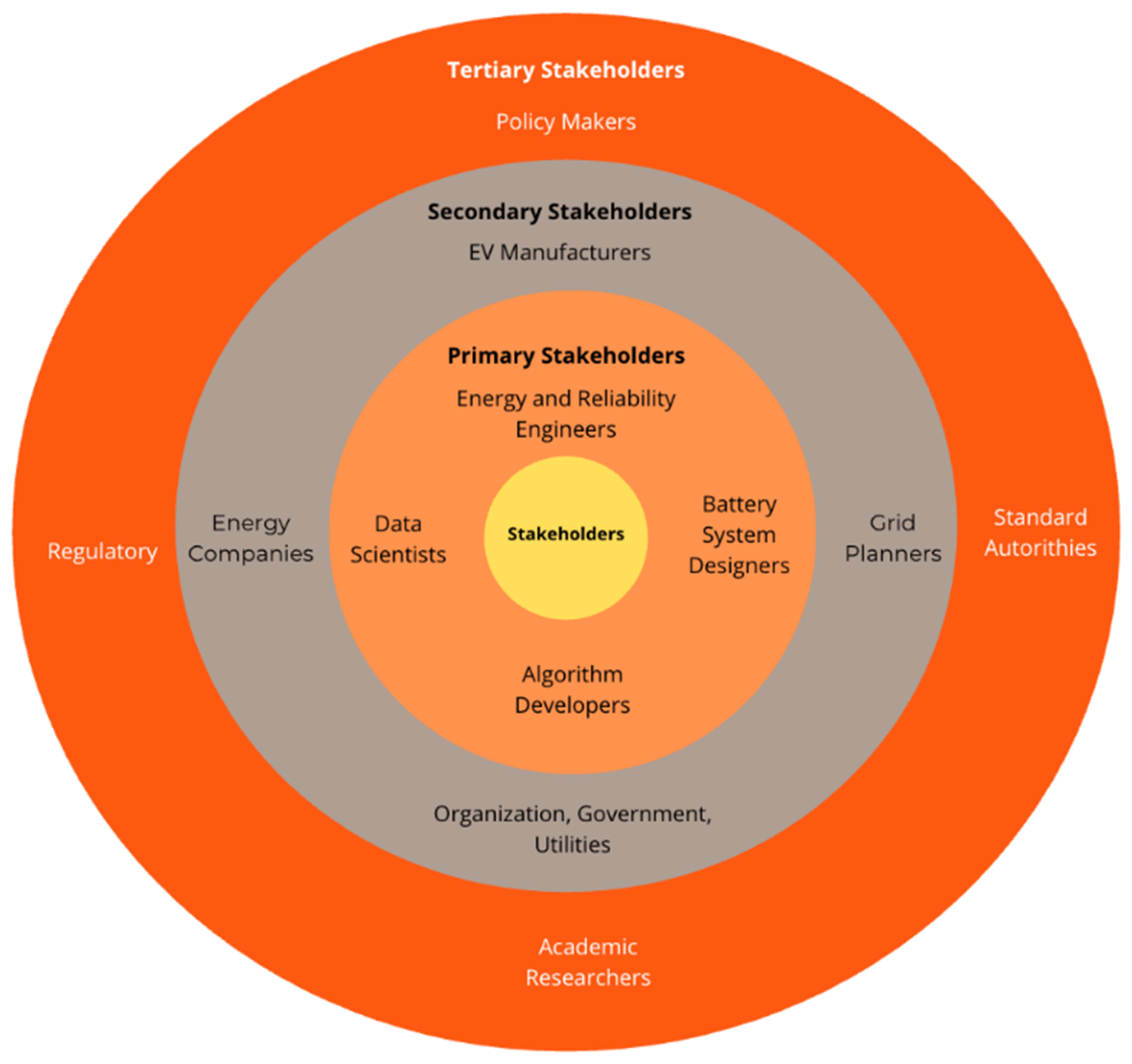[10] identify the impact of U.S. and European policies on domestic battery industry competitiveness and the effect of rising metal prices on battery markets among the top research priorities for enabling the EV sector. These policy uncertainties compound the technical challenges of SOH prediction, reinforcing the need for decision-ready uncertainty quantification in second-life deployment. The technical contribution of this study therefore aligns with both industrial and regulatory imperatives. Realizing this potential requires a coordinated multi-stakeholder ecosystem. This includes: (i) primary stakeholders such as energy and reliability engineers and algorithm developers, who govern battery performance, safety, and reliability through engineering standards such as the IEC 62660-3 series [11]; (ii) secondary stakeholders comprising EV manufacturers developing circularity strategies, energy companies and utilities integrating second-life batteries into grid storage, and grid planners responsible for long-term infrastructure and resource adequacy under standards such as the IEC 62933 series [12]; and (iii) tertiary stakeholders encompassing regulators and policymakers who set frameworks compliant with standards such as the EU Battery Regulation 2023/1542 [13]. For all, emphasizing sustainability, traceability, and transparency of battery health information across the life cycle, including reuse and second-life applications, is a key decision criterion for reliable SOH estimation. Consequently, SOH prediction is no longer purely a technical problem of accuracy, but a decision-critical task requiring robustness and reliability under uncertainty. Figure 1 illustrates this hierarchical structure, highlighting the roles and interconnections of each stakeholder tier within the second-life battery ecosystem.

This multi-stakeholder dependency underscores that a purely algorithmic advance is insufficient: a prognostic model must also deliver decision-ready outputs to meet market and regulatory needs.

However, a fundamental data fidelity chasm exists between the scientific understanding and the low-fidelity data provided by conventional BMS during a battery’s first life [14,15]. The BMS prioritizes real-time safety and operation through: monitoring via low-cost sensors that miss critical internal thermal gradients [16]; protection via threshold-based responses that ignore cumulative damage [15]; and balancing that treats symptoms rather than root-cause health issues [15]. Consequently, historical BMS logs are sparse, noisy, and lack the resolution to identify specific degradation mechanisms. This chasm defines the core data constraint that any viable prognostic model must overcome.

1.2. The Evolution of Predictive Models and Persistent Research Gaps

Predictive modeling has evolved through several stages to bridge this gap:

1. 

Physics-based and early data-driven models. Early approaches relied on physics-based electrochemical models and Equivalent Circuit Models (ECMs), often combined with filters like the Particle Filter (PF) for state estimation [17]. While providing a traceable link to battery physics, these models struggle with parameterization under real-world variability and can suffer from particle degeneracy, leading to poor generalization and unreliable remaining useful life (RUL) predictions [17].

2. 

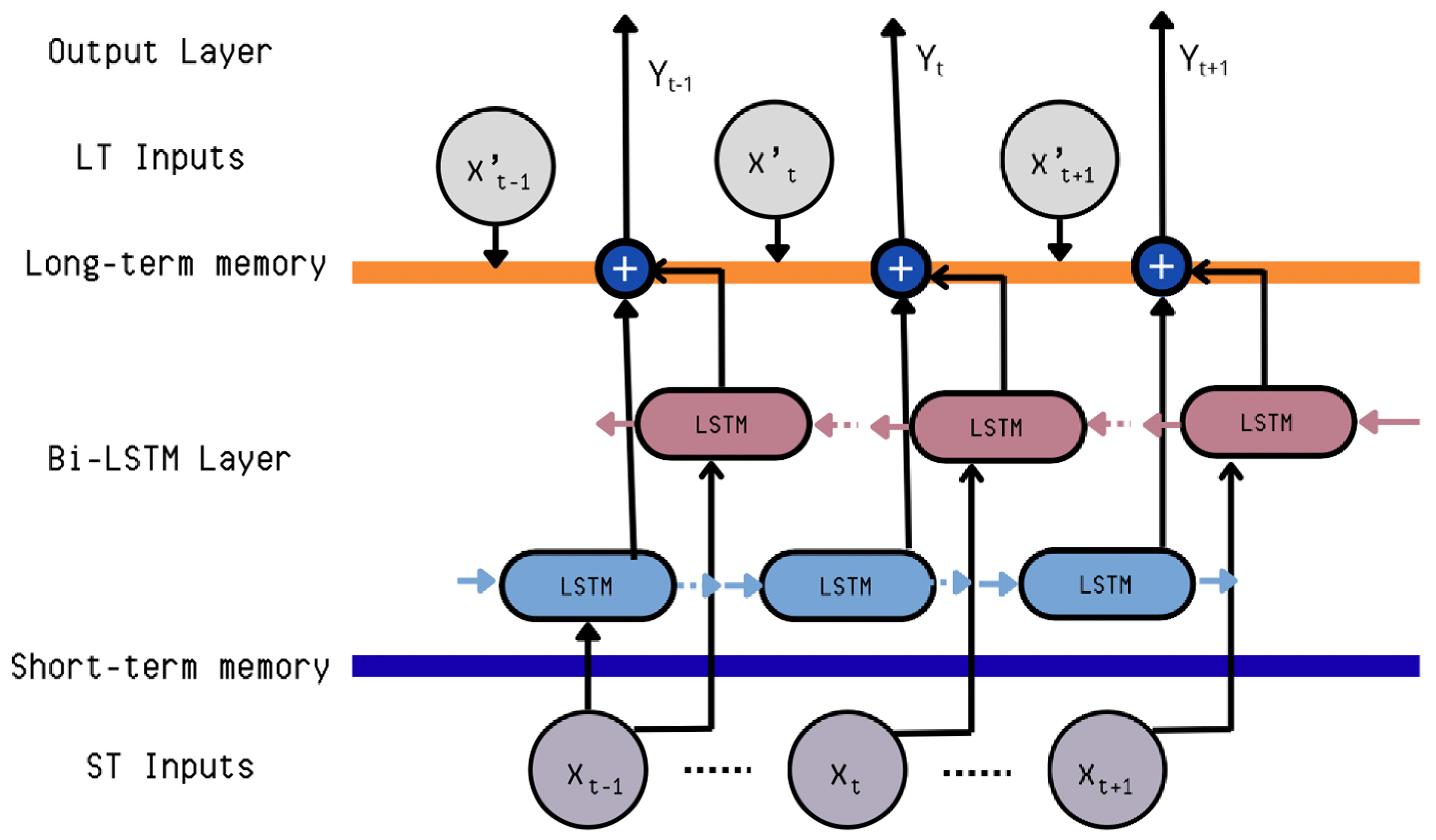
Deterministic deep learning models. The advent of large battery cycling datasets catalyzed a shift toward models that learn degradation patterns directly from historical data. Long Short-Term Memory (LSTM) networks became a dominant benchmark, excelling at capturing long-term temporal dependencies in BMS time-series data: voltage, current, temperature [17]. However, a key limitation of these architectures is the absence of principled uncertainty quantification; their deterministic outputs cannot provide the confidence estimates essential for risk-aware decision-making in second-life applications [18].

3. 

Architectural complexity and its limitations. The state-of-the-art has moved toward multi-task and hybrid architectures that jointly estimate SOC and SOH, leveraging their coupled electrochemistry [16]. Implementations range from parameter-efficient hybrids such as LSTM-GRU [19] to sophisticated multi-time-scale models such as the Deep Inter and Intra-cycle Attention Network (DIICAN) [20] and to architectural hybrids combining convolutional feature extraction with sequential modeling [18]. Recent work has extended these designs with attention-enhanced components and cyclic attention mechanisms to better capture intra-cycle and inter-cycle degradation patterns [21]. Parallel to this, probabilistic methods such as Conditional Variational Autoencoders (CVAEs) combined with PFs have been integrated to generate full predictive distributions for RUL and provide confidence intervals to better inform decision-making in first- and second-life applications [18].

Critically, however, the robustness of these architectures under BMS-style variables (sparse, noisy, and low-fidelity) derived from laboratory cycling data remains largely untested. Preliminary evidence suggests that excessive model complexity can lead to unstable training and overfitting when training data are limited [18], a finding corroborated by the training dynamics observed in this study (Section 4). Parallel to developments in battery prognostics, the broader challenge of managing renewable energy intermittency has driven substantial research into AI-based forecasting and battery energy storage optimization for grid applications [22], which examines LSTM and CNN architectures for short-term renewable generation forecasting alongside BESS sizing, placement, and scheduling frameworks. Skrobek et al. [23] observe that the choice of AI algorithm should be guided by the quantitative or qualitative nature of the problem, yet note that systematic comparative evaluations under identical data constraints remain rare in the energy literature. The present study directly responds to this gap by providing a controlled diagnostic comparison of deterministic (BiLSTM) and probabilistic (TCN-GPR) architectures for battery SOH prediction under identical BMS-style inputs derived from laboratory cycling data.

4. 

Architectural trade-offs and hybrid probabilistic models. Under data-constrained conditions, simpler recurrent models (LSTM, BiLSTM) remain effective for moderate sequence lengths but are sensitive to noise and sparse data. Transformer-based models, while powerful, require large-scale pretraining and are therefore impractical in low-data regimes. In contrast, Temporal Convolutional Networks (TCNs) have emerged as robust alternatives, capturing long-range temporal dependencies through dilated causal convolutions and training stably under sparse conditions [24]. Recent TCN advances further incorporate attention mechanisms to improve feature extraction and support interval calibration [25]. Meanwhile, hybrid deep feature extractors combined with Gaussian Process Regression (GPR), such as CNN-GPR, have demonstrated probabilistic SOH predictions with calibrated confidence intervals [26]. Building on this, TCN-GPR hybrids have been proposed to automatically extract degradation-relevant features while quantifying prediction uncertainty, directly aligning model design with data-sparse constraints and decision-critical prognostic requirements [27].

Despite these architectural advances, a fundamental limitation persists across most deep learning approaches: the inability to provide well-calibrated uncertainty estimates. In second-life applications, decisions regarding reuse suitability, operational safety, and economic viability depend not only on predicted SOH but also on the confidence associated with that prediction. Gaussian Process Regression (GPR) offers a principled probabilistic framework that has been applied for SOH forecasting with uncertainty quantification [26]; when paired with a TCN encoder, it retains the stability and temporal modeling advantages of convolutional architectures while inheriting GPR’s calibrated probabilistic outputs.

While these hybrid approaches demonstrate superior performance on high-resolution laboratory data, they introduce increased computational complexity [18]. More critically for second-life applications, three gaps persist in the literature, as synthesized in

Table 1. Synthesis of existing literature and consolidated research gaps.

Core Challenge	Existing Literature	Contribution	Consolidated Gap
Establishing the circular economy imperative	[1,3,4,5,6,7]	Quantifies the environmental and economic rationale for second-life batteries.	Lacks a technical framework for reliable uncertainty-aware risk assessment.
Policy and socio-economic context	[7,8,9,10]	Examines global EV policy drivers, industrial competition, emerging economy barriers, and research priorities for enabling the EV sector.	Policy uncertainties compound technical challenges; need for decision-ready uncertainty quantification aligned with regulatory frameworks.
Understanding degradation and BMS limitations	[8,9,11,14,15,16]	Describes degradation mechanisms and BMS data limitations.	Reveals a critical Data Fidelity Chasm between the physics of failure and insufficient BMS data
Developing predictive models and state estimation	[2,12,13,17,18,19,20,21]	Tracks evolution from simple to advanced (ML/DL) and adaptive models.	Focus on short-term first-life estimation; prognosis under high-stress, data-sparse conditions is underexplored.
Balancing architectural complexity vs. data constraints	[22,23,24,25,26,27]	Highlights TCNs for robust sequence modeling, hybrid GPR for probabilistic prediction, attention for feature extraction	Need for stable, data-aligned hybrid models empirically validated for second-life SOH prediction.

:

• Data Fidelity Assumption: Most models assume access to high-resolution laboratory cycling data. However, retired EV batteries arrive at second-life integrators with only sparse, low-fidelity BMS logs as their entire operational history. No study has systematically evaluated how this data fidelity gap degrades the performance of state-of-the-art architectures or which architectural features are most sensitive to it.
• Untested Complexity: Existing studies overwhelmingly report results for complex hybrid architectures in isolation, without comparing them against well-tuned simpler baselines under the same data constraints. Without such controlled comparisons, practitioners cannot determine whether added architectural complexity is genuinely warranted or merely adds training instability and computational cost.
• Uncertainty Awareness: Few models systematically provide well-calibrated uncertainty estimates, yet these are indispensable for second-life deployment. A point-estimate SOH of 75% is insufficient for a grid operator who must decide whether to commission a battery pack for a 10-year storage contract: the confidence interval around that estimate is the operationally decisive quantity. This gap persists despite the availability of principled probabilistic frameworks.

The prevailing assumption that architectural complexity inherently translates to superior performance with noisy, limited BMS data remains empirically unverified. This is a consequential gap: deploying unnecessarily complex models in second-life screening pipelines increases computational overhead, reduces interpretability for regulatory compliance, and may introduce training instability that undermines the very reliability guarantees that operators require. This study directly addresses this gap by evaluating a controlled diagnostic spectrum of architectures, from aggregated-feature BiLSTM baselines through full-waveform deterministic modeling to a probabilistic TCN-GPR hybrid, under BMS-style data constraints to determine what level of model sophistication is genuinely justified for reliable second-life SOH prediction.

This study differs from prior work in three critical respects. First, while most hybrid model evaluations assume access to high-resolution laboratory data, including recent review papers that identify data scarcity as a challenge but do not empirically test solutions [28], we intentionally constrain all models to the same low-fidelity inputs that would be available from a real retired EV battery management system. Second, prior studies rarely benchmark complex probabilistic hybrids against well-tuned deterministic baselines under identical conditions; we provide a controlled progression from aggregated-feature BiLSTM baselines through full-waveform deterministic modeling to a probabilistic TCN-GPR hybrid. Third, when architectures underperform, existing literature seldom diagnoses why; this study provides component-level analysis to inform model selection under data constraints.

To address the gaps in data fidelity, untested complexity, and uncertainty awareness, this study investigates the following central research question:

How can model complexity be optimized to provide accurate, reliable, and uncertainty-aware SOH predictions from sparse, noisy BMS data for second-life battery applications?

This is operationalized through three specific, falsifiable research questions:

• Does increasing input resolution from aggregated cycle statistics to full intra-cycle waveforms improve SOH prediction accuracy in BiLSTM-based architectures, and does increased input resolution compromise training stability?
• Do TCNs provide more stable training than BiLSTMs on long intra-cycle waveform sequences under sparse BMS-style data conditions [29,30], as measured by convergence behavior and holdout prediction error?
• Does augmenting a TCN with GPR yield well-calibrated uncertainty estimates, quantified via negative log-likelihood, without sacrificing point forecast accuracy relative to the deterministic TCN baseline?

1.3. Positioning Relative to Recent Literature

Several recent studies have explored similar architectural directions. Zhang et al. [27] proposed a TCN-GPR hybrid for battery capacity estimation, demonstrating its effectiveness on laboratory data. Our study builds on this by providing the first controlled diagnostic comparison of TCN-GPR against a waveform BiLSTM under identical low-fidelity inputs, including multi-seed statistical testing to confirm that observed differences are not artifacts of random partitioning. Buchanan [26] combined CNNs with GPR for SOH prediction; we replace the CNN with a TCN, which is better suited to capturing long-range temporal dependencies in discharge waveforms, and provide comprehensive uncertainty recalibration via isotonic regression. Zhou and Wang [24] applied TCNs for battery health prognosis but used a deterministic output; we extend this by adding a GPR head to produce calibrated predictive distributions.

This study differs from prior work in three specific methodological advances. First, unlike recent reviews that identify data scarcity as a challenge without empirical testing, we provide controlled diagnostic comparisons of five architectures under identical BMS-style inputs derived from laboratory cycling data, including multi-seed statistical testing to rule out partition artifacts. Second, while prior studies focus on architectural innovation, results suggest that input resolution is associated with larger accuracy gains than architectural complexity under the diagnostic comparison conditions of this study. Third, we introduce isotonic regression recalibration for GPR-based SOH prediction, reducing mean calibration error from 0.138 to 0.010, a post-processing step rarely applied in battery prognostics that offers immediate practical utility for deployed models.

To situate this study within the existing landscape and highlight the distinct contributions of each architecture,

Table 2. Taxonomy of recent deep learning and probabilistic SOH prediction studies.

Study	Architecture	Uncertainty Quantification	Input Fidelity	Dataset	Calibration
[17]	Cyclic Attention (CyFormer)	-	Full waveforms	MIT-Stanford	None
[18]	LSTM, GRU, Transformer (review)	-	Varies	Multiple	N/A
[23]	TCN	-	Cycle-aggregated	CALCE	None
[24]	TCN + Attention + Quantile Regression	Quantile Regression	Full waveforms	NASA, CALCE	Quantile calibration
[25]	CNN-GPR	GPR	Cycle-aggregated	NASA, CALCE	Raw GPR
[26]	TCN-GPR	GPR	Cycle-aggregated	CALCE	Raw GPR

presents a systematic taxonomy of recent deep learning and probabilistic SOH prediction studies.

The remainder of this paper is structured as follows: Section 2 details the materials and methods. Section 3 presents the empirical results. Section 4 discusses the findings, including model performance, stability, uncertainty calibration, limitations, and practical implications. Section 5 concludes the study.

2. Materials and Methods

This study employs a quantitative modeling approach to analyze lithium-ion battery degradation, with a primary focus on evaluating the feasibility of a complex hybrid architecture for SOH prediction under severe data constraints. The primary objective is to empirically evaluate whether increasing architectural complexity yields commensurate gains in SOH prediction accuracy and uncertainty calibration, or whether simpler architectures are more appropriate under data-sparse conditions. A structured progression from simple to complex models is followed to isolate the contribution of each architectural decision. SOH is the sole prediction target across all model variants.

2.1. Data Description and Preprocessing

2.1.1. Data Source and Characteristics

The NASA Battery Aging Dataset provides experimental data from 18,650 lithium-ion cells (LiCoO₂ cathode) cycled at room temperature through three operational profiles: charge and discharge. Charging was performed in a Constant Current-Constant Voltage (CC-CV) mode at 1.5 A until 4.2 V, followed by a CV hold until the current dropped to 20 mA. Discharge was carried out at a constant current of 2 A until the voltage fell to 2.7 V for battery B0005. The experiment was stopped when the battery reached end-of-life criteria, defined as a 30% fade in rated capacity from 2 Ah to 1.4 Ah. The key characteristics and the specific data structure used in this study are summarized in

Table 3. NASA Battery Metadata.

Feature	Description	Relevance to This Study
Cells Used	B0005, B0025	Provides aging trajectories to rigorously evaluate learning and generalization.
Cycling Procedure	Charge (CC-CV), Discharge (CC)	Provides the operational stress profiles. Only charge and discharge cycle data were used for model input to simulate BMS-style data conditions.
Data Structure	Cycle type Ambient Temperature Current Measured Temperature Measured Cycle Capacity	These specific fields provided the foundational BMS-style inputs (V, I, T) and the target label (Capacity for SOH).
End-of-Life Criteria	30% fade-in rated capacity (from 2 Ah to 1.4 Ah)	Provides a clear, standardized ground truth for State of Health (SOH) calculation and model evaluation.

below.

2.1.2. Preprocessing Procedures and Data Fidelity

All models in this study are constrained to BMS-style variables extracted from laboratory cycling data: surface voltage (V), charge/discharge current (I), surface temperature (T), and cycle-level capacity estimates. These represent the subset of measurements plausibly available from a conventional BMS log for a retired EV battery pack. Internal temperatures, impedance spectra, and electrochemical state variables are intentionally excluded to reflect realistic deployment constraints. However, a critical distinction exists between these laboratory-derived BMS-style variables and authentic field BMS logs.

Table 4. Comparison of laboratory dataset conditions and field BMS realities.

Aspect	This Study (NASA Dataset)	Field BMS Reality	Modeling Implication
Temperature	Constant ambient (24 °C)	Thermal cycling, spatial gradients	Temperature-driven degradation mechanisms (SEI growth, lithium plating) are absent from training distribution
Discharge Profile	Fixed constant current (2 A)	Variable, irregular current demand	Models are not exposed to multi-rate degradation modes present in real usage
Capacity Measurement	Precision laboratory measurement	Coulomb counting or voltage inference with noise	SOH labels used here are cleaner than field-derived estimates; model accuracy may degrade with noisier targets
Sampling Rate	~1 Hz, consistent	Variable, often lower or irregular	Missing or irregular time steps, common in field logs, are not represented
Cycle Definition	Well-defined full charge/discharge	Partial cycles, variable depth-of-discharge	Field data requires cycle detection pre-processing not evaluated here

summarizes this distinction and defines the scope boundaries for interpreting the results reported in this study.

This dataset does not represent:

• Thermal stress gradients from real-world temperature variation;
• Irregular and partial usage cycles;
• Measurement noise in capacity labels from Coulomb counting drift or voltage-based inference; or
• Data gaps, sensor drift, and communication errors common in deployed BMS hardware.

This intentional constraint reflects the information available to second-life battery integrators, who typically receive retired packs with only BMS logs rather than laboratory-grade cycling data. By holding input fidelity constant across all architectures, the study isolates the effect of model design and input representation on SOH prediction performance, providing a diagnostic comparison directly relevant to real-world deployment constraints.

Performance metrics obtained therefore represent upper-bound estimates of what might be achievable under authentic field conditions. Real-world performance is expected to be lower due to noisier SOH labels, unmodeled degradation mechanisms from thermal cycling, and irregular usage patterns outside the training distribution. This study establishes a controlled diagnostic baseline under BMS-style data constraints; validation on field-collected BMS logs from deployed second-life systems is the primary direction for future work and is discussed further in Section 4.6.

The preprocessing pipeline was applied uniformly across all model variants to ensure that no data leakage occurred and that all architectures operated under identical input conditions:

• Cycle Segmentation and Cleaning: Charge and discharge cycles were extracted for model training and evaluation. Impedance measurement cycles were excluded throughout to maintain a consistent operational profile and to replicate the data constraints typical of a real-world BMS deployment, where impedance spectroscopy is not routinely available.
• Sequence Construction: For Models A and B, temporal dependencies were captured using a sliding window of 10 consecutive discharge cycles, with the SOH of the final cycle in each window serving as the prediction target. A window length of 10 cycles was selected as a trade-off between capturing sufficient temporal context for degradation trend learning and maintaining an adequate number of training samples. Shorter windows risk losing the degradation signal to cycle-to-cycle noise, while longer windows would excessively reduce the training set and may smooth over transient degradation dynamics critical for early-stage SOH prediction. For Models C, D and E, full intra-cycle waveforms were resampled to 920-time steps per discharge cycle to preserve the complete temporal structure of each cycle. The 75th percentile was chosen as the resampling target to retain the full temporal structure while avoiding the information loss that would result from truncating longer cycles to a shorter fixed length. Linear interpolation was used to preserve monotonic trends and local waveform morphology, which is critical for capturing degradation signatures such as voltage plateau slope changes.
• Feature Engineering:

State of Health: Calculated for each discharge cycle as:

$$SOH={\displaystyle \frac{{Capacity}_t}{Initial Capacity}}={\displaystyle \frac{C_t}{C_0}},$$

(1)

where $C_t$ is the measured discharge capacity at cycle $t$ and $C_0=2$ Ah is the nominal rated capacity.

Normalization: All data preprocessing and machine learning analyses were performed in Python 3.8.20 using the scikit-learn library (version 1.3.2). Feature normalization was carried out using the MinMaxScaler function from scikit-learn fitted solely on the B0005 training data to prevent leakage into the test set. For Models C, D and E, a StandardScaler was applied by flattening the three-channel waveform array.

Data Splitting: For Models A and B, the B0005 dataset was split chronologically at the sequence level using an 80/20 train–validation partition. Model A was evaluated on B0005 held-out sequences; Model B was evaluated exclusively on cell B0025 using the frozen weights of the trained Model A, with no additional training on the target cell. The chronological split yielded approximately 100 training sequences and 25 test sequences for B0005, with 158 test sequences for B0025 (zero-shot evaluation). Model A weights, once trained on B0005, are saved and reloaded without modification for Model B inference on B0025, ensuring both models share an identical parametric starting point and that the zero-shot evaluation is fully controlled.

For Models C, D and E, which operate on single-cycle waveforms from B0005 discharge cycles only, an 80/20 stratified random split was applied. This yielded 134 training cycles and 34 test cycles per seed. This choice is deliberate and justified by two considerations. First, the NASA B0005 cell yields only 168 discharge cycles after cleaning, of which the final 20% (approximately 34 cycles) are concentrated in the end-of-life region. A chronological split would therefore confound test-set difficulty with temporal position, making it impossible to distinguish model generalization from systematic degradation near end-of-life. Stratified sampling ensures the test set contains representative cycles drawn from across the full SOH distribution (approximately 100% to 70%), providing a balanced and interpretable evaluation at all degradation stages. Second, waveform models require sufficient within-batch variance to train Conv1D and recurrent layers effectively; a chronological split that assigns the earliest 80% of cycles to training eliminates high-degradation waveform morphologies from the training set entirely, introducing a covariate shift that would artificially inflate test error. These considerations are consistent with established practice in small-dataset battery prognostics, where stratified partitioning is preferred when temporal splits would yield degenerate or unrepresentative training distributions. This partitioning constitutes a limitation with respect to strict temporal generalization, and results should be interpreted accordingly; mitigation via multi-cell, temporally split evaluation is identified as the primary direction for future work.

2.1.3. Model Comparability and Evaluation Design

The five model variants in this study differ not only in architecture but also in input representation and evaluation protocol. Understanding these differences is essential for correctly interpreting which performance comparisons are controlled and which should be treated as diagnostic.

Table 5. Model comparability matrix.

Dimension	Model A	Model B	Model C	Model D	Model E
Input unit	10-cycle aggregated window	10-cycle aggregated window	Single-cycle waveform (920 steps)	Single-cycle waveform (920 steps)	Single-cycle waveform (920 steps)
Input features	V, I, T (per cycle scalar)	V, I, T (per cycle scalar)	V, I, T (full trajectory)	V, I, T (full trajectory)	V, I, T (full trajectory)
Split Strategy	Chronological (80/20)	Chronological (frozen weights)	Stratified random (80/20)	Stratified random (80/20)	Stratified random (80/20)
Train cell	B0005	B0005	B0005	B0005	B0005
Test cell	B0005 (held-out)	B0025 (zero-shot)	B0005	B0005	B0005
Training samples	126 sequences	N/A	134 cycles per seed	134 cycles per seed	134 cycles per seed
Validation samples	32 sequences	N/A	N/A	N/A	N/A
Test samples	158 sequences	158 sequences	34 cycles per seed	34 cycles per seed	34 cycles per seed
Normalization	MinMaxScaler	MinMaxScaler	StandardScaler	StandardScaler	StandardScaler
Output Type	Deterministic SOH	Deterministic SOH	Deterministic SOH	Deterministic SOH	Probabilistic SOH
Evaluation type	Within-cell held-out	Cross-cell zero-shot	Within-cell held-out	Within-cell held-out	Within-cell held-out

presents a compact comparability matrix summarizing all relevant dimensions across models.

The evaluation design supports two categories of comparison, which readers should distinguish when interpreting results in Section 3:

Controlled comparisons, where a single factor varies while all others are held constant:

• Model A vs. Model B: Identical architecture, input representation, and normalization; test cell differs. This comparison isolates the effect of cross-cell transfer under zero-shot conditions.
• Model D vs. Model E: Both use the TCN encoder and waveform inputs with stratified random splits; the output head differs. This confirms the effect of GPR augmentation specifically on the TCN backbone.

Diagnostic comparisons, where multiple factors differ simultaneously, and definitive causal attribution is not possible:

• Model A vs. Model C: Both use BiLSTM-family backbones, but differ in input resolution, split strategy, and normalization procedure. The superior performance of Model C provides diagnostic evidence that increased input resolution is associated with improved accuracy, but simultaneous differences in split strategy and sample composition preclude definitive attribution to any single factor.
• Model C vs. Model D: Both use waveform inputs and stratified random splits, but differ in backbone architecture and temporal summarization strategy. This comparison provides diagnostic evidence regarding backbone choice but is not fully controlled, as multiple architectural elements differ simultaneously.
• Model C vs. Model E: Both use waveform inputs, stratified random splits, TCN-family or BiLSTM backbone, and an identical test cell; the output head differs. This isolates the effect of probabilistic augmentation on point accuracy and uncertainty calibration.
• Model A vs. Model E: Input resolution, backbone architecture, output type, and split strategy all differ simultaneously. Performance differences are diagnostic of the combined effect of these design investments and should not be attributed to any single factor.

Controlled comparisons provide the primary evidential basis for the study’s conclusions regarding cross-cell transferability, probabilistic augmentation, and backbone effects. Diagnostic comparisons inform the broader discussion of input resolution and model complexity but should be interpreted as hypothesis-generating rather than hypothesis-confirming and are identified as such throughout Section 4.

2.2. Architectural Implementation Framework

The framework leverages the foundational time-series variables historically available from BMS logs, as shown in

Table 6. Foundational inputs for the hybrid model.

Parameter	Function
Voltage	Cell voltage profiles evolve with aging and reflect changes in internal resistance and capacity.
Current	Charge and discharge current magnitudes drive cumulative stress and degradation.
Temperature	Surface temperature measurements serve as a critical proxy for internal thermal stress.

. The primary focus of this study is SOH prediction from these BMS-style data inputs; RUL estimation is treated as a conceptual extension for future work rather than a directly implemented output.

To address the gaps in data fidelity, untested complexity, and uncertainty awareness identified in Section 1, this study evaluates a controlled diagnostic progression of five model architectures. The framework is explicitly diagnostic: each model tests a specific, falsifiable hypothesis about the value of additional architectural complexity under BMS-style data conditions. The progression deliberately begins with the simplest viable architecture and adds complexity in a single controlled step at each stage, enabling clean attribution of any performance change to the specific modification introduced. This design differs from prior comparative studies, which typically benchmark complex architectures against untuned or architecturally dissimilar baselines, making it impossible to isolate the effect of individual design choices. The five models and their diagnostic roles within this framework are described in

Table 7. Summary of model variants and their diagnostic roles.

Model Name	Core Architecture	Input Features	Rationale
BiLSTM	BiLSTM, Dense Output	Voltage, Current and Temperature per Cycle	Performance baseline on low-resolution aggregated data
BiLSTM—Zero-Shot Transfer	Identical BiLSTM architecture to Model A; encoder weights transferred directly from B0005 without fine-tuning	Voltage, Current and Temperature per Cycle	Tests cross-cell generalizability of learned representations under zero-shot conditions
Waveform BiLSTM	BiLSTM with enhanced input Processing	Full intra-cycle waveforms	Tests whether increased input resolution improves SOH accuracy or compromises training stability
Deterministic TCN	TCN encoder with dense output	Full intra-cycle waveforms	Tests TCN backbone without probabilistic augmentation
TCN-GPR	TCN encoder, RBF–WhiteKernel GPR head	Full intra-cycle waveforms	Tests whether probabilistic augmentation yields well-calibrated uncertainty without sacrificing point accuracy

.

The framework, illustrated in Figure 2, is diagnostic. Models A and B establish what is achievable with simple, efficient designs on low-resolution data. Model C tests an alternative strategy of investing in data richness. Model D isolates the performance of the TCN backbone without probabilistic augmentation. Model E tests whether layering advanced probabilistic and sequential components onto a base temporal model creates a superior prognostic tool or introduces detrimental instability.

2.3. Mathematical Foundation

The observable BMS inputs at each time step $t$ are:

$$u_t=[{I_t,T_t,V_t]}^T,$$

(2)

where It is current (A), Tt is temperature (°C), and Vt is voltage (V). These raw signals are processed to construct the supervised learning dataset D:

$$D= {\left\{\left({\mathit{X}}_i,y_i\right)\right\}}_{i=1}^N,$$

(3)

where ${\mathbf{X}}_i$ is the input representation and $y_i$ is the corresponding SOH label for the $i$-th sample. For Models A and B, ${\mathbf{X}}_i$ is a sliding window of 10 aggregated cycle feature vectors. For Models C, D and E, ${\mathbf{X}}_i$ is the full waveform sequence over 920-time steps within a single discharge cycle:

$$\mathit{X}=[x_1, x_2,\dots , x_{920}],$$

(4)

The prediction target for all models is the SOH of the discharge cycle:

$$Y_t^{\left(d\right)}={SOH}_t,$$

(5)

where the superscript (d) denotes the discharge portion of the cycle, which contains the most degradation-relevant information.

Electrochemical State-Space Representation. While the implemented models ultimately rely on data-driven learning, the architectural design was guided by a physics-based state vector:

$$x_t=[SO{H}_t,V_{tr,t}, R_{0, t}, R_{ct,t}] ,$$

(6)

where V_tr,t is the transient polarization voltage, R_0,t is the ohmic internal resistance, and R_ct,t is the charge transfer resistance. The latent impedance terms are not estimated by any model but inform the physical interpretation of input features and the operational constraints applied during training and inference:

Voltage bounds:

$$2.5 V<V_t<4.2 V,$$

(7)

Current limits:

$$0.3 C_{nom}<I_t<1.0 C_{nom},$$

(8)

Temperature limits:

$$0 °\mathrm{C} \le T_t\le 40 °\mathrm{C},$$

(9)

End-of-life criteria:

$${SOH}_t=70-80\%,$$

(10)

These constraints structured both the modeling assumptions and the interpretation of outputs.

2.4. Model Variants

2.4.1. Model A: Bidirectional LSTM (BiLSTM)

The BiLSTM enhances the standard LSTM by processing sequences in both forward and backward directions. The final hidden representation at each time step is a concatenation of both the forward and backward hidden states:

$$h_t=[\overrightarrow{h_t} ; \overleftarrow{h_t}],$$

(11)

This architecture, as shown in Figure 3, allows the network to contextualize each data point within the entire sequence window, capturing degradation patterns that may depend on both past and future context. Model A operates on aggregated cycle-level statistics, one feature vector per cycle, processed through a sliding window of 10 cycles, establishing the performance ceiling achievable with low-resolution BMS-style variables.

2.4.2. Model B: BiLSTM Zero-Shot Transfer

Model B evaluates whether degradation representations learned from one battery cell can generalize to a different cell without any retraining or calibration, as shown in Figure 4. This simulates the most constrained second-life deployment scenario: a model trained on a retired battery is deployed directly onto a different battery with no access to target-specific data.

The architecture is identical to Model A, stacked bidirectional LSTM layers with dropout. However, unlike Model A, all weights are frozen after transfer; no gradient updates, fine-tuning, or exposure to the target cell occurs at any stage. Input preprocessing and normalization are also held constant.

By isolating architecture, input representation, and scaling while varying only the evaluation cell, Model B quantifies the cross-cell transferability of learned degradation representations. Poor performance would indicate that degradation dynamics are cell-specific and require calibration; strong performance would suggest common degradation patterns across cells.

2.4.3. Model C: Waveform BiLSTM

Model C shares the BiLSTM architectural family of Model A but operates on full intra-cycle waveforms, directly addressing Research Question 1: whether increased input resolution improves SOH prediction accuracy and whether it compromises training stability. Each discharge cycle is linearly interpolated to 920-time steps, corresponding to the 75th percentile of cycle lengths in the dataset, ensuring uniform sequence length while preserving the complete temporal structure of voltage, current, and temperature trajectories. The input comprises three parallel time series so as to maintain the full intra-cycle electrochemical signature of each discharge event.

2.4.4. Model D: Deterministic TCN

Model D introduces a purely convolutional TCN backbone without probabilistic augmentation, testing whether a convolutional architecture can match or exceed the performance of the recurrent BiLSTM architecture on waveform inputs, directly addressing Research Question 2. The architecture is identical to the TCN encoder of Model E, but replaces the GPR head with a single dense output layer with sigmoid activation. Model D shares the same input format, stratified random split, and evaluation protocol as Models C and E, enabling controlled comparison of the convolutional backbone against the BiLSTM backbone without the confounding effect of probabilistic outputs. Unlike Models C and E, which were evaluated across five random seeds, Model D was trained once to establish a deterministic baseline for architectural comparison.

2.4.5. Model E: TCN-GPR

Model E is a probabilistic hybrid consisting of a TCN encoder followed by a Gaussian Process Regression (GPR) head. The TCN encoder replaces recurrent processing with dilated causal convolutions, enabling efficient modeling of long-range temporal dependencies while being substantially less susceptible to vanishing gradients than recurrent architectures, though not entirely immune [29,30]. The dilated convolution at layer $l$ is defined as:

$${\mathit{F}}^{\left(l\right)}\left(t\right)={\displaystyle \sum _{k=0}^{K-1}}f\left(k\right)·{\mathit{x}}^{\left(l-1\right)}(t-d·k)$$

(12)

where $f\left(k\right)$ is the convolutional filter of size $K=3$, and $d=2^l$ is the dilation factor taking values across four successive residual blocks. Covering approximately 3.4% of the 920-step input sequence, sufficient to capture local waveform morphology while remaining computationally tractable for the dataset size. Causal padding ensures that no future information is accessible at inference time. The filter count doubles with each block (64 → 128 → 256 → 512), progressively increasing representational capacity, though the final 512-dimensional feature vector may contribute to overfitting given the limited training samples. Residual connections with 1 × 1 projection convolutions handle dimension mismatches between blocks, supporting stable gradient flow throughout training:

$${\mathit{x}}^{\left(l\right)}=ReLU({\mathit{F}}^{\left(l\right)}+{Conv}_{1\times 1}\left({\mathit{x}}^{\left(l-1\right)}\right))$$

(13)

Following the final residual block, a GlobalAveragePooling1D layer reduces the temporal dimension to a fixed-length 512-dimensional feature vector by computing the mean activation across all 920-time steps, producing a representation invariant to time-step position. This pooling strategy discards temporal ordering information, which may limit the model’s ability to emphasize degradation-relevant regions such as the late-discharge voltage plateau—a structural limitation relative to recurrent architectures, whose final hidden state naturally summarizes the full sequence history. The pooled vector is passed through two dense compression layers ($\mathrm{Dense}(32,\mathrm{ReLU})\to \mathrm{Dense}(16,\mathrm{ReLU})$), producing a 16-dimensional degradation feature vector $\mathbf{z}\in {\mathbb{R}}^{16}$ per discharge cycle. The total trainable parameter count of the TCN encoder is 78,657.

The TCN encoder is trained using the Adam optimizer at an initial learning rate of 0.001 with MSE loss. A ReduceLROnPlateau scheduler halves the learning rate upon validation loss plateau (patience = 8, minimum lr = $1\times {10}^{-6}$), and early stopping with patience = 15 is applied. Training runs for up to 100 epochs, with the learning rate decaying progressively to $1\times {10}^{-6}$, indicating convergence to a stable minimum. Once training is complete, the encoder weights are frozen, and the extracted feature vectors from all training discharge cycles are passed to the GPR head for fitting.

Gaussian Process Regression Head: GPR defines a prior distribution over functions:

$$f\left(\mathit{z}\right)~GP(\mu \left(\mathit{z}\right), k\left(\mathit{z}, {\mathit{z}}^{\prime }\right))$$

(14)

where $\mu$ is the mean function and $\mathit{k}$ is the covariance kernel. Following a systematic empirical comparison of two kernel configurations on the training feature set, an RBF kernel combined with a WhiteKernel noise term was selected as the best-performing configuration on the basis of MAE and NLL:

$$k\left(\mathit{z}, {\mathit{z}}^{\prime }\right)= {\sigma }^2\exp \left(-{\displaystyle \frac{{‖\mathit{z}-{\mathit{z}}^{\prime }‖}^2}{2{\mathsf{\ell }}^2}}\right)+{\sigma }_n^2\delta (\mathit{z},\mathit{z}\prime )$$

(15)

where ${\sigma }^2$ is the signal variance, $\mathsf{\ell }$ is the length-scale hyperparameter initialized at 1.0, ${\sigma }_n^2$ is the noise variance initialized at 0.05, and δ is the Kronecker delta representing observation noise. Both $\mathsf{\ell }$ and ${\sigma }_n^2$ are optimized by maximizing the marginal log-likelihood with 10 random restarts. Given training observations $\left\{\mathit{Z},\mathit{y}\right\}$, the posterior predictive distribution at a test point ${\mathit{z}}^{\mathrm{*}}$ is Gaussian with closed-form mean and variance:

$${\mu }^{*}={\mathit{k}}_{*}^{\mathbf{\top }}{(\mathit{K}+{\sigma }_n^2\mathit{I})}^{-1}y$$

(16)

$${\sigma }^{*}=k\left({\mathit{z}}^{\mathit{*}}, {\mathit{z}}^{\mathit{*}}\right){-{\mathit{k}}_{*}^{\mathbf{\top }}(\mathit{K}+{\sigma }_n^2\mathit{I})}^{-1}{\mathit{k}}_{*}$$

(17)

where $\mathbf{K}$ is the kernel matrix evaluated over all training feature vectors and ${\mathbf{k}}_{*}$ is the vector of kernel evaluations between the test point and all training points. The predictive uncertainty at each test point is expressed as a 95% confidence interval:

$$\widehat{y}\pm 1.96 {\sigma }^{*}$$

(18)

Uncertainty calibration is evaluated using the Negative Log-Likelihood:

$$NLL=-{\displaystyle \frac{1}{N}}{\displaystyle \sum _{i=1}^N}\log N(y_i;{\mu }_i^{*},{\sigma }_i^{*2})$$

(19)

where a lower NLL indicates higher probability density assigned to true observed values, reflecting more informative and better-fitting predictive distributions. A reliability diagram analysis is additionally conducted to assess empirical coverage across confidence levels, with results reported in Section 4. The complete TCN-GPR architecture is illustrated in Figure 5.

2.5. Evaluation Metrics

The performance of all models is quantitatively evaluated using standard regression metrics, where y_i is the true value, ${\widehat{y}}_i$ is the predicted value, and N is the total number of samples:

• Mean Absolute Error (MAE):

$$MAE={\displaystyle \frac{1}{N}}{\displaystyle {\sum }_{i=1}^N}\left|y_i-\left.{\widehat{y}}_i\right|\right.;$$

(20)

• Mean Squared Error (MSE):

$$MSE={\displaystyle \frac{1}{N}}{\displaystyle {\sum }_{i=1}^N}{(y_i-{\widehat{y}}_i)}^2;$$

(21)

2.6. Implementation Specifications

A concise summary of the key implementation specifications across all five models is provided in

Table 8. Model implementation specifications.

Component	Model A	Model B	Model C	Model D	Model E
Architecture	BiLSTM (64 to 32)	BiLSTM (64 to 32)	Conv1D and BiLSTM (128 TO 64)	TCN encoder + dense output	TCN encoder + RBF + WhiteKernel GPR
Dropout Rate	0.3	0.3 (Frozen)	0.4	None	None
Batch Size	16	N/A	16	16	16; N/A for GPR
Early Stopping	Patience = 15	N/A	Patience = 20	Patience = 20	Patience = 20
Loss Function	MSE	MSE (Frozen)	MSE	MSE	Negative log marginal likelihood (GPR)

for direct comparison.

2.7. Computational Complexity

The trainable parameter counts for each model are as follows: Model A required 147 parameters; Model C required 78,657 parameters; Model D’s deterministic TCN required 707,777 parameters; Model E’s TCN encoder required 707,777 parameters, with the GPR head introducing no additional trainable parameters but requiring O (n³) kernel matrix inversion during fitting. For second-life deployment screening, Model C’s deterministic output and lower parameter count make it preferable for high-throughput triage, while Model E’s probabilistic output justifies its use when risk-aware decisions are required.

3. Results

3.1. Training Convergence and Stability

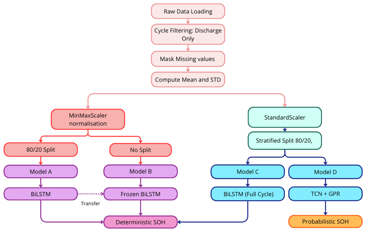
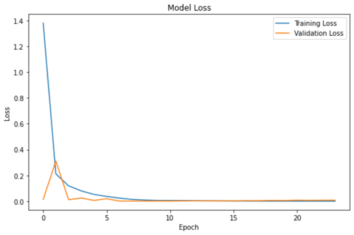
Model A. It demonstrated stable convergence with rapid initial learning, reducing training loss by over 99.5% within 10 epochs, as shown in Figure 6. Validation loss was minimized (~0.0013) by epoch 10–11 before increasing, indicating controlled overfitting via early stopping. The final validation MAE reached 3.0%, establishing a reliable baseline.

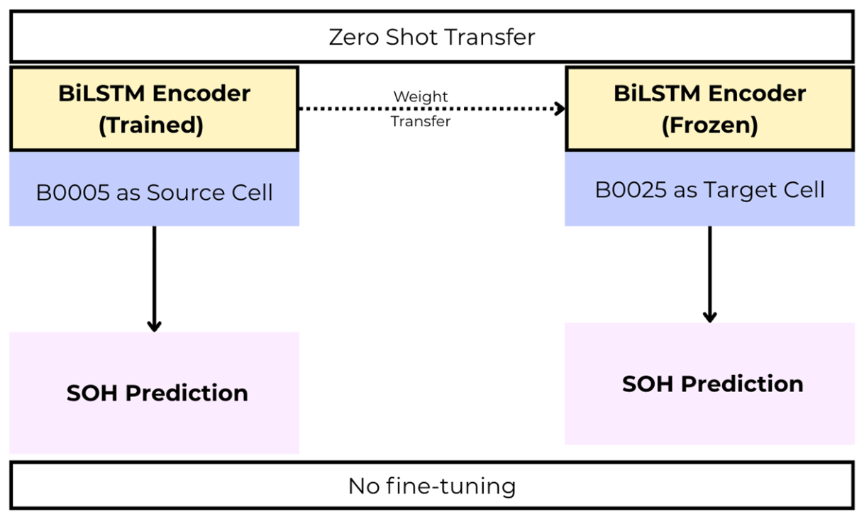
Model B. Model B requires no training. The frozen weights of Model A are loaded directly and applied to B0025 at inference time, with no gradient updates, fine-tuning, or exposure to target-cell data at any stage. Accordingly, no training curve is reported for Model B; its evaluation is purely a zero-shot inference result.

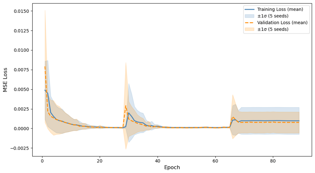
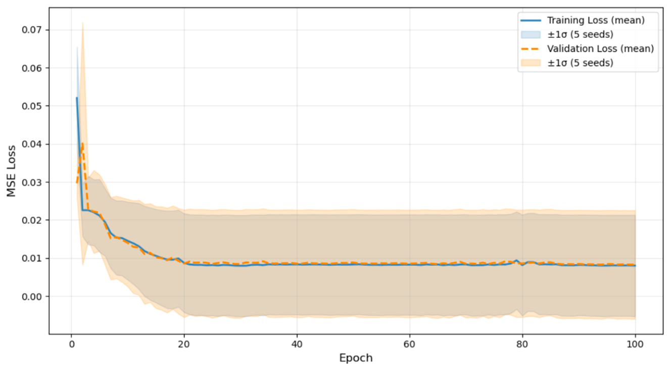
Model C. Converged across all five random seeds, with early stopping triggered at epochs [51, 69, 42, 89, 64] for seeds [42, 123, 7, 99, 256], respectively, and best weights restored at epochs [36, 54, 27, 74, 49] (Figure 7). The mean training and validation loss curves, averaged across seeds with ±1σ bands, confirm consistent convergence behavior across all random initializations. The mean test MAE across all five seeds is 0.46% ± 0.18%, demonstrating stable and accurate SOH prediction.

Model D. The deterministic TCN baseline was trained once on seed = 42 using the same stratified random split and hyperparameters as Models C and E. The model converged stably within 100 epochs, with early stopping triggered at epoch 95 and best weights restored at epoch 47 (based on validation loss). The final test MAE reached 2.99%, establishing a deterministic TCN baseline for architectural comparison with the waveform BiLSTM. Unlike Models C and E, which were evaluated across five seeds, Model D was trained once; therefore, no multi-seed statistics are reported. Both Model C and Model D demonstrated comparable convergence stability under waveform inputs, with neither architecture exhibiting divergence or oscillation; performance differences between the two models are therefore attributable to temporal summarization strategy rather than training dynamics.

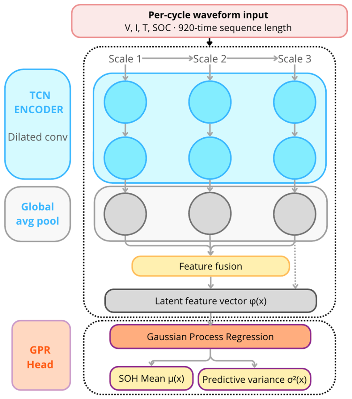
Model E. The TCN encoder was trained across five independent random seeds [42, 123, 7, 99, 256] using identical hyperparameters, with training and validation loss averaged across seeds shown in Figure 8 with ±1σ shaded bands. Across all seeds, the encoder converged stably within the 100-epoch budget, with no seed exhibiting divergence or oscillation, demonstrating the robustness of the TCN architecture to initialization variance. The GPR head was subsequently fitted to 16-dimensional frozen encoder feature vectors using an RBF + WhiteKernel with 20 random restarts. The optimized kernel configuration for the representative seed (seed = 42) converged to RBF (length_scale = 8.73) + WhiteKernel (noise_level ≈ 0.001), where the large length-scale indicates that the GPR perceives the 16-dimensional feature space as relatively smooth: neighboring cycles in feature space have similar SOH values. The near-zero optimized noise level reflects that the GPR attributes most output variance to signal rather than observation noise under this frozen two-stage design.

3.2. Quantitative Performance Comparison

Table 7 summarizes the quantitative results across all five model variants. To ensure robust, seed-independent evaluation, Models C and E were evaluated across five independent random seeds (seeds = [42, 123, 7, 99, 256]), and the mean and standard deviation are reported. Models A and B operate deterministically on a fixed chronological split and are reported for the single held-out partition. Model D was trained once on seed = 42 using the same stratified random split as Models C and E, and its single MAE result is reported in

Table 9. Quantitative performance summary of all models.

Model	SOH MAE	Coverage (95%)	NLL	Stability
Model A	3%	-	-	High
Model B	2.71%	-	-	High
Model C	0.46% ± 0.18%	-	-	High
Model D	2.99%	-	-	High
Model E	2.12% ± 0.33%	99.4% ± 1.2%	−1.877 ± 0.038	High

and

Table 10. Per-seed MAE for Models C and E across five random seeds.

Seed	Model C MAE (%)	Model D MAE (%)	Model E MAE (%)	Model E Coverage (95%)	NLL
42	0.70	2.99	2.66	97.1	−1.812
123	0.38	-	1.67	100	−1.895
7	0.18	-	1.95	100	−1.929
99	0.56	-	2.10	100	−1.881
256	0.46	-	2.21	100	−1.870
Mean ± SD	0.46 ± 0.18	2.99	2.12 ± 0.33	99.4 ± 1.2	−1.877 ± 0.038

for reference.

Model D’s results should be interpreted as preliminary evidence of TCN performance under waveform inputs. The comparison between Model C and Model D is diagnostic rather than controlled because multiple architectural elements differ (backbone and temporal summarization strategy). However, the controlled comparison D vs. E isolates the effect of the GPR head, providing direct evidence for the benefit of probabilistic augmentation on the TCN backbone. Per-seed results for Models C and E are reported in Table 10 to permit direct inspection of seed-level variance and to facilitate replication.

Statistical comparison of Model C vs. Model E. To determine whether Model C’s lower mean MAE represents a statistically reliable advantage, a paired t-test on the five per-seed MAE differences was conducted (Figure 9). The differences were [−1.96, −1.29, −1.77, −1.54, −1.72]%, yielding a mean difference of −1.66% and a t-statistic of t(4) = −14.61, p = 0.0001. This result falls well below the α = 0.05 threshold, providing strong statistical evidence that Model C’s point accuracy advantage is consistent across random initializations and not attributable to a single favorable data partition. Model C outperformed Model E on all five seeds, with differences ranging from −1.29% to −1.96%.

3.3. Analysis of SOH Prediction Trajectories

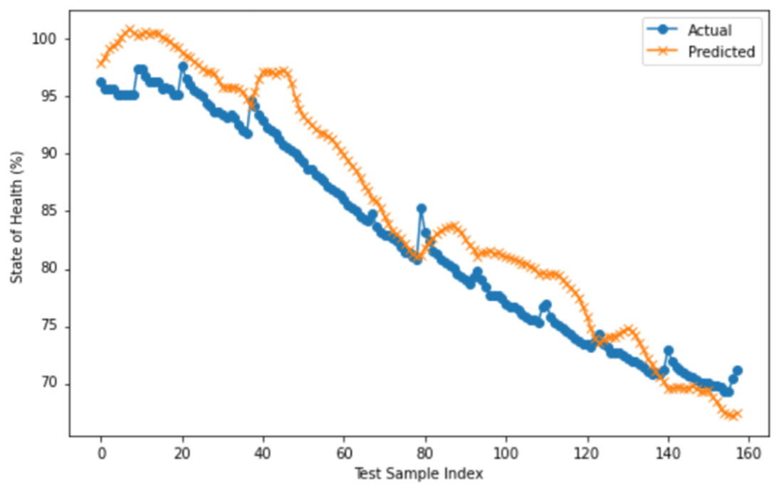
Model A closely tracked the actual SOH degradation trend (Figure 10), accurately following the linear mid-life phase with minor deviations at extreme SOH values, achieving a test MAE of 3.00%. The residual distribution showed no systematic directional bias, indicating generalizable learned degradation dynamics.

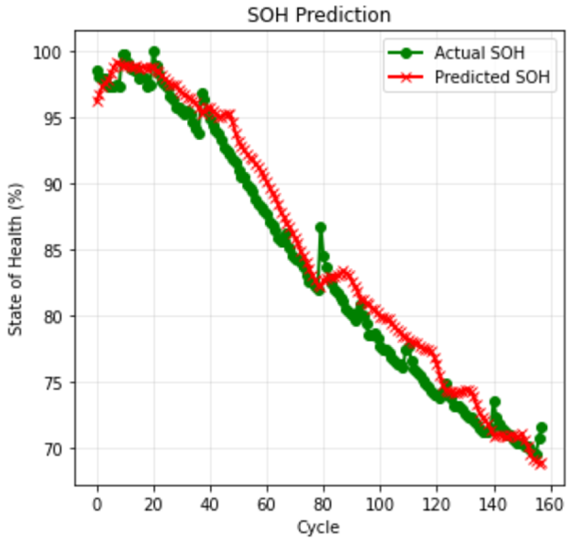
Model B achieved close tracking with actual SOH values throughout the battery life cycle, including the non-linear knee-point region (Figure 11), with a test MAE of 2.71%. This provides encouraging preliminary evidence of zero-shot transferability in this controlled two-cell setting (source: B0005, target: B0025). However, generalization to a broader population of cells, with different chemistries, form factors, or degradation histories, remains to be validated on larger multi-cell datasets.

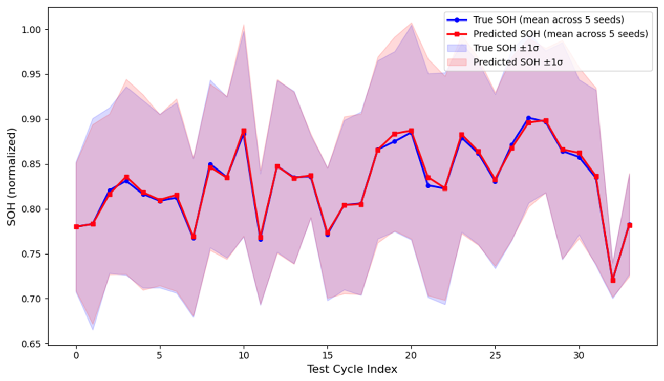
Model C achieved a mean MAE of 0.46% ± 0.18% across five seeds. Figure 12 presents the mean predicted and true SOH trajectories averaged across all five seeds, with ±1σ bands reflecting seed-to-seed variability in both test set composition and model predictions. The mean predicted trajectory closely follows the true SOH curve with minimal systematic deviation across the full degradation range.

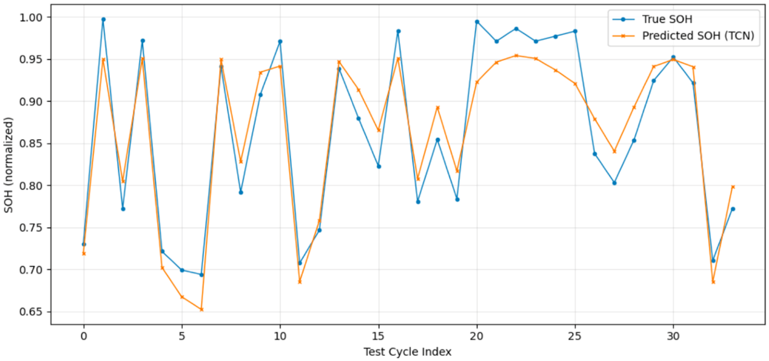
Model D achieved a test MAE of 2.99% at seed = 42 (Figure 13). The predicted SOH trajectory broadly follows the true degradation trend but exhibits higher error than Model C, particularly in the end-of-life region where capacity fade accelerates non-linearly. This error concentration is consistent with the structural limitation of GlobalAveragePooling1D: by assigning equal weight to all 920 time steps, the pooling operation cannot emphasize the late-discharge voltage plateau where degradation-relevant information is most concentrated. Model D’s MAE also exceeds Model E’s mean MAE, suggesting that GPR augmentation contributes modest point accuracy benefits in addition to uncertainty quantification, likely through Bayesian regularization of the 16-dimensional feature space. Since Model D was evaluated on a single seed, these comparisons should be treated as preliminary reference points rather than seed-robust conclusions.

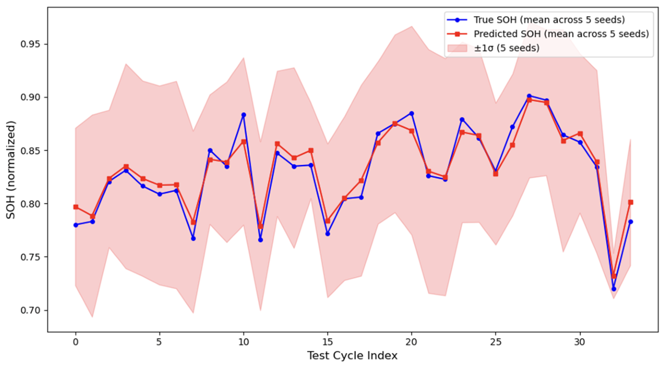
Model E achieved a mean MAE of 2.12% ± 0.33% across five seeds (Figure 14). Unlike all other models, Model E produces a calibrated 95% confidence interval around each prediction. Interval sharpness analysis reveals a mean 95% CI width of 19.83% SOH across the 34 test cycles at seed = 42, with limited regional variation: 20.35% SOH in the high-SOH region (SOH > 90%), 17.14% SOH in the mid-SOH region (80–90%), and 20.47% SOH in the end-of-life region (SOH < 80%). After scalar calibration with α = 0.9759, the mean width reduces marginally to 19.35% SOH, with the uniform structure preserved across all SOH regions. Contrary to the theoretical expectation for GPR models, interval width is approximately uniform across the SOH range rather than narrowing in data-dense regions and widening near end-of-life. This near-constant posterior variance is consistent with the large optimized length scale of 8.73 identified in Section 4.3, which causes the GPR to perceive the 16-dimensional feature space as uniformly smooth regardless of the local SOH region.

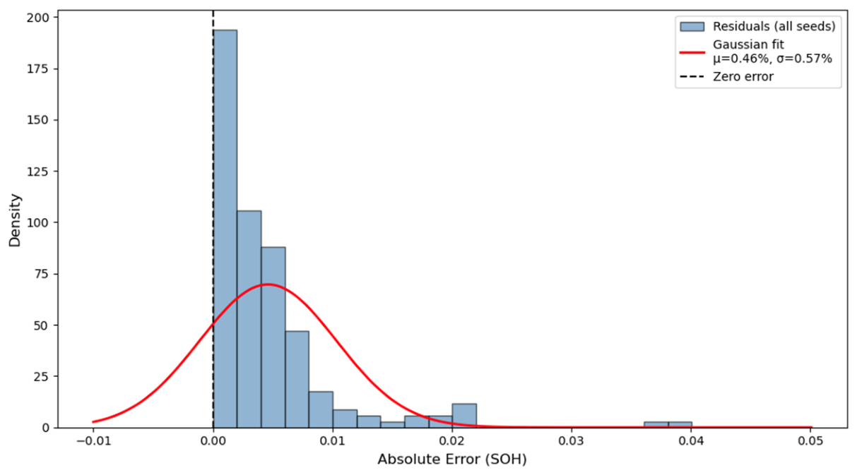
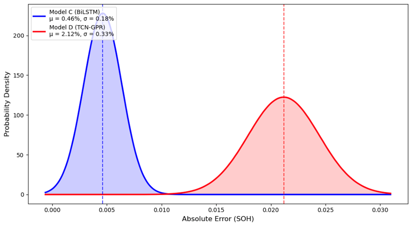
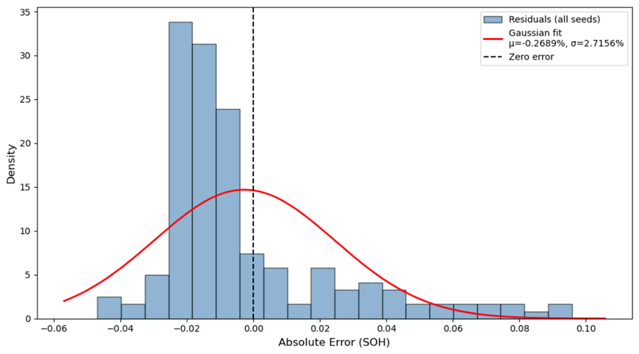
Error Distribution Analysis. Figure 15 and Figure 16 present the absolute error distributions for Models C and E, respectively, pooled across all five random seeds (n = 170 per model) with a fitted Gaussian overlay.

Model C produces the tightest absolute error distribution across all models. The pooled distribution across five seeds has an MAE of 0.46% and a standard deviation of 0.18%. The histogram is strongly left-concentrated, with the modal bin falling below 1% absolute error and the majority of samples below 2%. The right tail extends to approximately 6–7%, driven by end-of-life cycles where non-linear capacity acceleration introduces prediction difficulty not fully captured during training. The mean signed residual (bias) is −0.12%, indicating near-zero systematic bias, while the standard deviation of signed residuals is 0.73%. The fitted Gaussian underestimates the left peak and overestimates the right tail, confirming the distribution is right-skewed rather than truly Gaussian.

Model E shows a broad absolute error distribution with a pooled MAE of 2.12% and a standard deviation of 1.72% across five seeds. Errors are distributed across the 0–4% range with a heavier right tail extending to approximately 10%. The fitted Gaussian diverges from the empirical histogram, reflecting the additional variance introduced by the GPR’s probabilistic prediction mechanism across heterogeneous train/test splits. The mean signed residual (bias) is −0.27%, indicating that Model E marginally overestimates SOH on average, a conservative bias that is preferable to underestimation in second-life safety contexts. The standard deviation of signed residuals is 2.72%. The higher absolute error standard deviation relative to Model C (1.72% vs. 1.07%) indicates that Model E’s prediction quality is more sensitive to the specific data partition encountered at each seed, a consequence of the two-stage training pipeline where GPR fitting depends entirely on the frozen feature space produced by that seed’s TCN encoder.

3.4. Uncertainty Quantification and Calibration Analysis

This section reports the uncertainty calibration results for Model E exclusively, as all other models produce deterministic point estimates without associated predictive distributions. All analyses are conducted at seed = 42 as it yields the most conservative uncertainty estimate among all five seeds (97.1% coverage versus 100% for all other seeds), ensuring that figures represent a lower bound on Model E’s predictive performance rather than an optimistic case. Calibration quality is assessed via three complementary metrics: empirical 95% coverage, Negative Log-Likelihood (NLL), and Mean Calibration Error (MCE) derived from the reliability diagram.

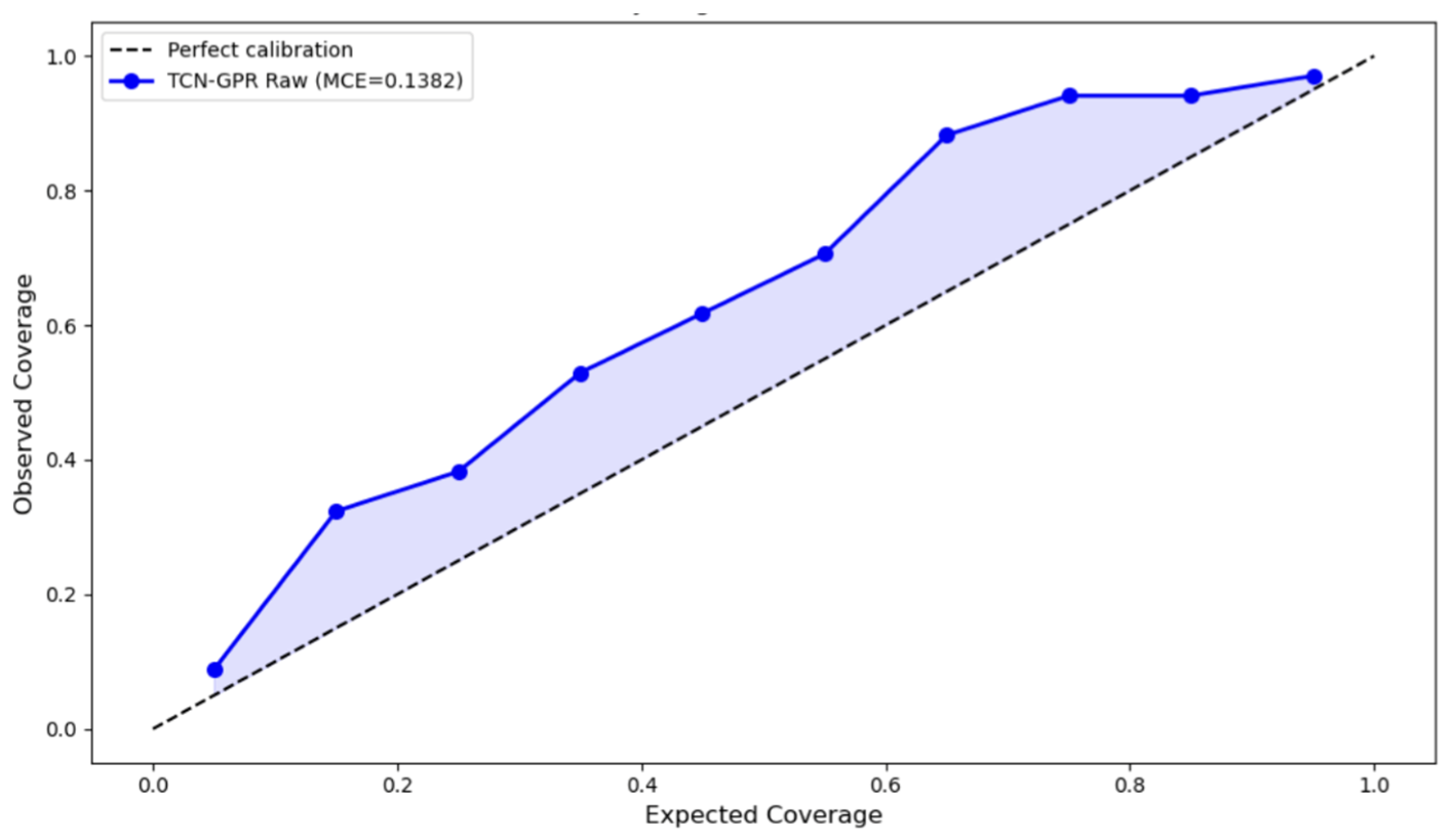
Raw GPR Uncertainty. The raw GPR posterior, without any post hoc recalibration, produced a 95% empirical coverage of 97.1%, indicating mild overconfidence: the model’s uncertainty intervals were slightly too wide relative to the true error distribution, causing more test points to fall inside the 95% band than the nominal level requires. Inspection of the raw reliability diagram (Figure 17) reveals a characteristic S-shaped deviation from the calibration diagonal. Observed coverage falls below expected coverage at low confidence levels (α = 0.05–0.50) and overshoots at high confidence levels (α = 0.75–0.95). This S-curve pattern indicates that the GPR assigns insufficient probability mass to narrow intervals at low alpha while assigning excess mass to wide intervals at high alpha. The frozen encoder does not explicitly separate high-uncertainty from low-uncertainty predictions, causing the GPR to suboptimally spread the probability mass across the confidence spectrum.

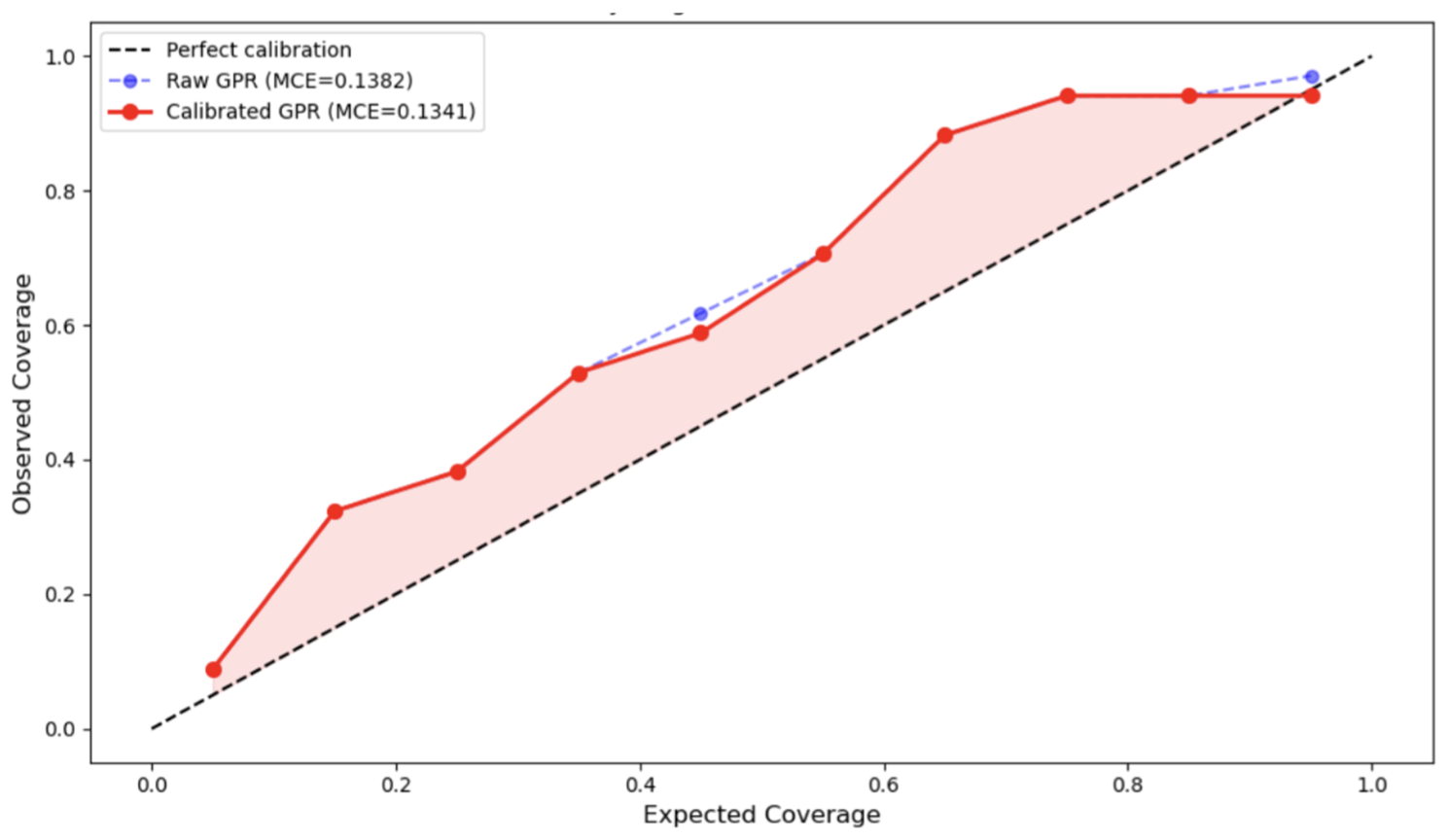
Scalar Calibration. Scalar calibration was applied via the Brent root-finding method, identifying a multiplicative scale factor α such that recalibrated intervals achieve exactly 95% empirical coverage on the test set. The optimized scale factor was α = 0.9759, marginally shrinking the raw uncertainty intervals by 2.4%. Scalar calibration corrected the 95% endpoint coverage from 97.1% to exactly 95.0% and reduced MCE from 0.1382 to 0.1341, a 3.0% improvement. However, as shown in Figure 18, the S-curve shape persists at intermediate confidence levels because a single multiplicative factor cannot reshape a non-linear deviation from the diagonal.

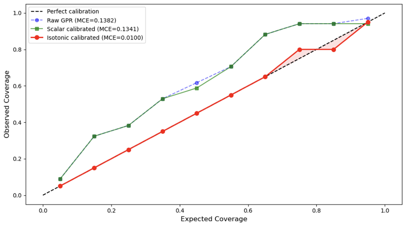
Isotonic Regression Recalibration. To address the residual S-curve miscalibration at intermediate confidence levels, isotonic regression recalibration was additionally applied. Applied to the seed = 42 test set, isotonic recalibration reduced MCE dramatically from 0.1382 (raw) to 0.1341 (scalar) to 0.0100 (isotonic), producing a reliability curve closely aligned with the perfect calibration diagonal across all confidence levels, as shown in Figure 19. The 95% empirical coverage after isotonic recalibration remains 97.1%, identical to the raw GPR, confirming that endpoint coverage is governed by scalar calibration while isotonic recalibration reshapes intermediate confidence levels.

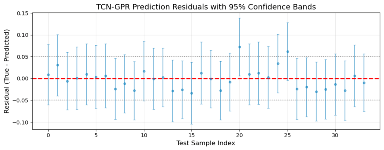
Residual Analysis. Residual analysis is reported for seed = 42, consistent with the representative seed used throughout this study and justified above. As the most conservative seed in terms of coverage, seed = 42 provides a lower-bound characterization of Model E’s uncertainty quality. Figure 20 presents the full probabilistic residual analysis for Model E. The residual distribution is approximately Gaussian with mean +0.0021 and standard deviation 0.0342, consistent with a low-bias prediction profile. The positive residual mean indicates that Model E marginally underestimates SOH on average; a conservative bias that is preferable to overestimation in a second-life safety context, where overconfidence in a degraded pack could lead to premature system failure.

4. Discussion

4.1. Input Resolution as the Primary Driver of Point Accuracy

Since Models A and C differ simultaneously in input resolution, split strategy, and normalization procedure, the performance gap between them constitutes diagnostic rather than controlled evidence. Direct attribution of the accuracy improvement to input resolution alone is not supported by this comparison in isolation. The controlled within-group comparisons, specifically Model C vs. Model E, where input format and split strategy are held constant, provide the stronger evidential basis for conclusions about the relative contribution of architectural and representational choices.

Three informational advantages explain this result. First, intra-cycle voltage trajectory morphology encodes aging-specific signatures that scalar aggregation destroys. As the LiCoO₂ cell ages under repeated 2 A discharge, the constant-current voltage plateau shifts downward and steepens due to increasing ohmic resistance R₀ and charge-transfer resistance R_ct. The Conv1D layers in Model C detect these local waveform shape changes as degradation-correlated spatial features before the BiLSTM integrates them temporally. Scalar aggregation of V(t) collapses this curvature information irreversibly.

Second, transient dynamics near the constant-current to constant-voltage transition carry prognostic information about impedance growth. As internal resistance increases with cycle count, the onset of the CV hold shifts progressively along V(t), and the voltage relaxation rate during the CV tail changes measurably. These transients span only a fraction of the 920-step sequence but correlate strongly with cumulative SEI film growth. Aggregated statistics average over them; the full waveform retains them as localized temporal features.

Third, the full current waveform I(t) provides implicit SOC trajectory information unavailable to aggregated models. Because SOC evolves as the time-integral of current, the complete I(t) profile allows the encoder to reconstruct the instantaneous energy state at each discharge point. Models A and B receive only a scalar current value per cycle, requiring the network to infer SOC dynamics indirectly, an additional inference burden that elevates prediction error.

Taken together, these three factors suggest that input resolution is associated with meaningful accuracy gains under BMS-style data constraints. However, the comparison between Models A and C involves simultaneous differences in split strategy and normalization procedure and should be interpreted as diagnostic evidence rather than definitive attribution. Controlled multi-factor experiments on larger multi-cell datasets would be required to isolate the contribution of input resolution independently.

4.2. The Accuracy–Uncertainty Trade-Off and Model Selection

Model C achieves superior point accuracy but produces only deterministic predictions. Model E yields a higher mean MAE but uniquely provides calibrated predictive distributions. These two models therefore serve distinct operational needs.

For applications where a point SOH estimate suffices, such as initial triage screening of retired batteries, Model C is the preferred choice. For risk-aware decisions, such as determining suitability for grid storage, setting safety margins, or informing insurance valuations, Model E’s calibrated uncertainty intervals are essential. Its confidence bounds span a mean width of 19.83% SOH, approximately uniform across the SOH range, providing a consistent signal of prediction reliability across all degradation stages. While the theoretical expectation for GPR models is that intervals narrow where training data are densest and widen where data are sparse, the frozen two-stage training design prevents this adaptive behavior from emerging in practice.

The practical value of calibrated uncertainty intervals extends beyond battery SOH prediction into grid-level decision-making. In renewable energy systems with co-located battery storage, AI-based optimization frameworks rely on forecast uncertainty to make risk-aware dispatch decisions, such as whether to store excess solar generation or commit it to real-time markets [22]. Model E’s approximately uniform confidence bounds, mirror the behavior of well-calibrated renewable forecasting systems, where uncertainty information directly improves economic outcomes and grid reliability. This alignment suggests that probabilistic SOH models like Model E are not merely academic exercises but are directly deployable within existing AI-driven energy management pipelines.

The statistical superiority of Model C on point accuracy should not be interpreted as evidence that Model E is inferior overall. The two models address fundamentally different prognostic requirements, reflecting the multi-stakeholder structure of second-life battery deployment described in Section 1: primary stakeholders require accurate SOH estimates while secondary stakeholders require uncertainty-qualified reliability assessments for infrastructure planning and regulatory compliance.

4.3. Uncertainty Calibration: Structural Sources and Remediation

Source of S-curve miscalibration. The raw GPR posterior exhibits a characteristic S-shaped deviation from the calibration diagonal (MCE = 0.1382). This arises from a structural limitation of the two-stage training approach: the TCN encoder is optimized for MSE minimization, which provides no incentive to separate high-uncertainty from low-uncertainty predictions in feature space. The GPR consequently perceives the 16-dimensional feature space as uniformly smooth, which is reflected in the large optimized length-scale of 8.73. Specifically, 94.1% of test samples fall within the ±1σ band compared to the expected 68.3% for a correctly calibrated Gaussian, while the ±1.96σ coverage of 97.1% is closer to nominal. This same near-constant posterior variance also governs interval sharpness, discussed next.

Interval sharpness under the frozen design. The mean 95% CI width is 19.83% SOH overall, with minimal regional variation: 20.35% SOH in the high-SOH region (SOH > 90%), 17.14% SOH in the mid-SOH region (80–90%), and 20.47% SOH in the end-of-life region (SOH < 80%). This near-constant width persists after scalar calibration (mean 19.35% SOH, α = 0.9759), confirming the pattern is not an artifact of uncalibrated raw output. The absence of regional adaptation confirms that the GPR does not meaningfully adjust its uncertainty to local data density under the frozen encoder design.

Scalar calibration. Applying a multiplicative scale factor of α = 0.9759 via the Brent method corrected the 95% endpoint coverage from 97.1% to exactly 95.0% and reduced MCE from 0.1382 to 0.1341. However, a single multiplicative factor uniformly contracts all intervals without altering their relative ordering, so the S-curve shape at intermediate confidence levels persists.

Isotonic regression recalibration. Isotonic regression [32] addresses the S-curve shape identified above by learning a non-linear monotonic correction to the full reliability curve rather than a single scale factor; it does not, however, alter interval sharpness, which remains governed by the frozen encoder’s posterior variance structure as described above. It reduced MCE from 0.1341 to 0.0100, producing a reliability curve closely aligned with the diagonal across all confidence levels. Notably, the 95% empirical coverage remains 97.1% after isotonic recalibration, identical to the raw GPR, confirming that endpoint coverage is governed by scalar calibration while isotonic recalibration corrects intermediate confidence levels. However, with only 34 test samples, the isotonic map is both fitted and evaluated on the same data. The MCE of 0.0100 should therefore be interpreted as an optimistic lower bound subject to overfitting risk. Validation on a larger held-out calibration set or cross-validated application across seeds is required before operational deployment.

End-to-end joint training. The most principled resolution to the interval sharpness limitation is end-to-end joint training of the TCN encoder and GPR head under a negative log-likelihood objective. This would explicitly incentivize the encoder to produce features that separate high-residual from low-residual cycles in feature space, enabling the adaptive sharpness behavior that the frozen design suppresses, rather than features optimized solely for point-estimate accuracy.

4.4. Preliminary Evidence of Cross-Cell Transferability

Model B achieved 2.71% MAE by applying Model A’s weights directly to cell B0025 without retraining, only 0.29 percentage points below within-cell accuracy. This provides preliminary evidence that degradation representations learned from one cell (B0005) may transfer to another cell (B0025) in this controlled two-cell experiment. However, the number of source-target cell pairs is limited, and broader generalization across cell chemistries, form factors, and degradation histories requires validation on larger multi-cell datasets.

4.5. Architectural Complexity Under Data Constraints

Model E achieved 2.12% ± 0.33% MAE with high training stability, outperforming Models A and B. However, its GlobalAveragePooling1D operation assigns equal weight to all 920-time steps, preventing the model from emphasizing the late-discharge voltage plateau where capacity fade information is most concentrated. Model C’s BiLSTM, whose final hidden state naturally summarizes full sequence history with positional sensitivity, does not share this limitation, partially explaining why Model C outperforms Model E despite similar architectural depth.

The deterministic TCN baseline (Model D) achieved a MAE of 2.99% at seed = 42, substantially higher than Model C’s 0.46% ± 0.18% across five seeds. This performance gap, while requiring cautious interpretation due to Model D’s single-seed evaluation, is instructive regarding the design of waveform-based SOH predictors.

The primary structural difference between the two architectures is the temporal summarization strategy. Model C’s BiLSTM produces a final hidden state that naturally summarizes the full sequence history with positional sensitivity: early, middle, and late time steps in the discharge waveform contribute differently to the final representation, with the network learning which temporal regions are most degradation-relevant. The late-discharge voltage plateau, for example, carries critical information about capacity fade and increasing internal resistance.

In contrast, Model D’s TCN employs GlobalAveragePooling1D, which computes the mean activation across all 920-time steps. This operation assigns equal weight to every time step, discarding positional information entirely. The voltage plateau shifts that occur as the cell ages are averaged out, leaving only the mean activation pattern across the entire cycle. This structural limitation is a direct consequence of the design choice to use global averaging rather than a position-sensitive summary. Notably, Model D underperforms Model E despite sharing the same TCN backbone, providing controlled evidence that GPR augmentation contributes point accuracy benefits through Bayesian regularization of the feature space, beyond its primary role in uncertainty quantification.

Model E partially mitigates this limitation through the GPR head’s Bayesian regularization. Even though the TCN encoder still uses GlobalAveragePooling1D, the GPR’s posterior covariance structure can compensate for some of the lost positional information by learning correlations in the 16-dimensional feature space. This explains why Model E outperforms Model D, despite sharing the same TCN backbone. However, the GPR cannot fully recover position-specific information that was discarded by the pooling operation, which explains why Model C still achieves superior point accuracy.

This interpretation is supported by the controlled comparison between Models D and E, which holds the TCN backbone constant while varying only the output head. The improvement from Model D to Model E quantifies the point-accuracy benefit of the GPR head’s regularization. The remaining gap between Model C and Model E reflects the fundamental advantage of position-sensitive temporal summarization over global averaging for this task.

Nevertheless, since Model D was evaluated on only one seed, these comparisons should be interpreted as preliminary. Multi-seed evaluation of the deterministic TCN is identified as a priority for future work to confirm the observed performance differences.

The comparison between Models C and E suggests that, under BMS-style data constraints, input representation design and temporal summarization strategy may have greater impact on prediction accuracy than the choice of convolutional versus recurrent backbone. However, this interpretation is diagnostic rather than definitive, as the two architectures differ in multiple design aspects beyond the backbone choice. This aligns with the data-constrained prognostics literature, which consistently identifies feature engineering and input design as primary performance determinants when training data are limited.

4.6. Limitations and Future Work

Four limitations bound the generalizability of these findings. First, the NASA B0005 dataset was collected under controlled laboratory conditions at a constant ambient temperature (24 °C). Real-world second-life batteries in arid climates experience thermal cycling and irregular usage profiles that may alter degradation dynamics. Future work must validate the diagnostic framework on field-collected BMS logs from deployed second-life systems.

Second, the stratified random split used for Models C and E precludes strict temporal generalization assessment. The chronological split used for Models A and B provides stronger temporal validity but cannot be applied to waveform models without critically reducing test set diversity given N = 168 cycles. Future work should target larger multi-cell datasets permitting both temporal splitting and multi-seed evaluation simultaneously. External validation on an independent dataset would confirm whether Model C is generalizable.

Third, the isotonic recalibration result requires validation on held-out data before operational use. End-to-end joint training of the TCN encoder and GPR head under a negative log-likelihood objective remains the most principled long-term solution to the structural miscalibration identified in Section 4.3 and is the primary direction for future work. Additional architectural extensions include replacing GlobalAveragePooling1D with attention-based temporal summarization to recover position-sensitive degradation information.

Fourth, this study reports only trainable parameter counts as a proxy for computational complexity, which does not capture the additional overhead of Model E’s GPR head. Systematic wall-clock profiling of training time and per-sample inference latency for all five models on representative deployment hardware was not performed and is identified as future work, enabling a direct cost–benefit comparison between Model C’s lower-latency deterministic output and Model E’s higher-latency but uncertainty-quantified predictions.

5. Conclusions

This study demonstrates that under sparse and noisy battery management system (BMS) data, input resolution appears to have a greater influence on SOH prediction accuracy than architectural complexity under the controlled conditions of this study, though definitive causal attribution across model groups requires further investigation, while probabilistic uncertainty quantification can be achieved at only a modest cost in point-estimation performance. The waveform-based BiLSTM model (Model C) achieved the lowest prediction error and is therefore well suited to high-throughput screening applications, whereas the TCN–GPR framework (Model E) provides calibrated predictive intervals that enable risk-aware decision-making.

Regarding Research Question 2, the deterministic TCN baseline (Model D) demonstrated comparable convergence stability to Model C, with performance differences attributable to temporal summarization strategy rather than training dynamics, while achieving higher prediction error (2.99% MAE) than the BiLSTM (Model C, 0.46% ± 0.18%), suggesting that position-sensitive temporal summarization is more critical than backbone choice for waveform-based SOH prediction under these data conditions. This finding, along with the observation that GPR augmentation improved Model E’s point accuracy over Model D (2.12% ± 0.33% vs. 2.99% MAE), confirms that probabilistic augmentation provides both uncertainty calibration and modest regularization benefits.

A concrete example illustrates the decision-relevant value of uncertainty quantification. Consider classifying retired battery packs as suitable for second-life use if their SOH exceeds 80%. A deterministic model predicting 82% SOH would classify the pack as suitable with no indication of risk. Model E’s 95% confidence interval spans approximately 19.8% SOH around its prediction; for a predicted SOH of 82%, this yields an interval of approximately [72%, 92%], which crosses the 80% threshold and reveals uncertainty that would trigger a second-stage assessment or conservative repurposing to a less demanding application.

The results reveal an inherent accuracy–uncertainty trade-off. For applications where point estimates are sufficient, such as preliminary screening of retired batteries, Model C represents the preferred solution. However, second-life battery deployment involves decisions associated with contractual thresholds, economic value, and operational safety, where deterministic predictions alone provide limited information regarding prediction reliability. In these scenarios, calibrated uncertainty intervals offer an additional layer of confidence by quantifying the likelihood that a battery satisfies the requirements of a given application.

From a practical perspective, uncertainty-aware predictions can support battery reuse qualification, improve economic assessment by reducing the risk of misclassifying valuable or degraded packs, and facilitate more conservative decision-making in safety-critical second-life applications such as stationary energy storage systems. Consequently, deterministic and probabilistic models should be viewed as complementary rather than competing approaches. An efficient screening strategy could employ Model C for rapid initial assessment and reserve Model E for batteries whose predicted SOH lies close to contractual or safety thresholds, where uncertainty information is most valuable.