Hybrid Particle Whale Optimization for Dual-Output EV Fast-Charging Parameter Estimation

Abstract

High-voltage electric-vehicle (EV) fast charging requires accurate coordination between the off-board charger and the battery management system during voltage and current negotiation. This study evaluates a Hybrid Particle Swarm Optimization-Whale Optimization Algorithm (HPWOA) schedule for training a dual-output feedforward neural network that directly estimates ChargePower_kW and ChargeCurrent_A. Ten protocol-state and battery-condition variables were used as inputs. The 158-dimensional neural-weight vector was optimized using 75 Particle Swarm Optimization (PSO) iterations, followed by 75 Whale Optimization Algorithm (WOA) iterations. Using the supplied 500-record dataset, a reproducible 30-seed sample-level evaluation was conducted with a common 3775 fitness-function-evaluation budget for PSO, the WOA, the SFSA, and the HPWOA. The Stochastic Fractal Search Algorithm (SFSA), therefore, used 30 iterations because it evaluates five diffusion candidates per individual. The reported HPWOA mean ± standard deviation (SD) was RMSE = 4.658 ± 0.986 kW and R² = 0.843 ± 0.071 for power, and RMSE = 12.686 ± 2.687 A and R² = 0.858 ± 0.059 for current. The HPWOA outperformed the WOA and SFSA, but not standalone PSO. A conventional mini-batch Adam-trained dual-output neural network produced RMSE = 1.704 ± 0.121 kW and 4.946 ± 0.273 A, and R² = 0.980 ± 0.003 and 0.979 ± 0.002, respectively. Charger-grouped five-fold validation gave the HPWOA R² = 0.857 ± 0.045 (power) and 0.873 ± 0.048 (current). An analytical P = V × I reconstruction was physically consistent in construction and did not show a statistically significant power–RMSE difference from direct HPWOA outputs. The results, therefore, position the two-phase schedule as a reproducible comparative baseline rather than as a demonstrated replacement for gradient-based training or a physically constrained reconstruction.

1. Introduction

The rapid growth of battery-electric vehicles (BEVs) has intensified the need for fast, reliable, and battery-safe charging technologies [1]. While electric mobility provides important benefits in terms of lower tailpipe emissions, reduced dependence on fossil fuels, and improved integration with future smart-grid systems [2], large-scale BEV adoption also introduces new technical challenges for charging infrastructure, power-electronics control, grid stability, and battery lifetime management [3]. Among these challenges, high-voltage DC fast charging is particularly important because it must deliver high charging power within a short time while ensuring that the battery pack remains within safe electrical, thermal, and electrochemical operating limits. Modern DC fast chargers commonly operate within the 150–350 kW range and rely on structured communication with the on-board battery management system (BMS) during charging negotiation [4]. In CHAdeMO-based charging, the charger and BMS exchange charging permission, voltage, current, and safety-related information before and during power delivery [5]. In the Combined Charging System (CCS), high-level communication enables the EV and the charger to negotiate charging limits, connector status, and charging-state information [6]. Similarly, GB/T-based fast-charging systems define communication and control procedures for matching charger output capability with battery-pack requirements [7]. In these protocol-driven systems, the charger announces its capability, the BMS reports the battery condition, and both systems converge on safe voltage and current setpoints [8]. The demanded voltage, ${\mathrm{D}\mathrm{e}\mathrm{m}\mathrm{a}\mathrm{n}\mathrm{d}\mathrm{V}\mathrm{o}\mathrm{l}\mathrm{t}\mathrm{a}\mathrm{g}\mathrm{e}}_{\mathrm{V}},$ and demanded current, ${\mathrm{D}\mathrm{e}\mathrm{m}\mathrm{a}\mathrm{n}\mathrm{d}\mathrm{C}\mathrm{u}\mathrm{r}\mathrm{r}\mathrm{e}\mathrm{n}\mathrm{t}}_{\mathrm{A}},$ therefore, represent the requested charging targets, while the realized charging power, ${\mathrm{C}\mathrm{h}\mathrm{a}\mathrm{r}\mathrm{g}\mathrm{e}\mathrm{P}\mathrm{o}\mathrm{w}\mathrm{e}\mathrm{r}}_{\mathrm{k}\mathrm{W}},$ and the realized charging current, ${\mathrm{C}\mathrm{h}\mathrm{a}\mathrm{r}\mathrm{g}\mathrm{e}\mathrm{C}\mathrm{u}\mathrm{r}\mathrm{r}\mathrm{e}\mathrm{n}\mathrm{t}}_{\mathrm{A}},$ represent the actual electrical quantities delivered to the battery pack [9]. In practice, the demanded and delivered values may differ because of battery internal resistance, converter limitations, temperature-dependent derating, communication delay, or charger–BMS compatibility effects [10,11,12,13,14]. Thus, predictive estimation of realized charging parameters has become a critical requirement for intelligent EV fast-charging operation. Accurate prediction of ${\mathrm{C}\mathrm{h}\mathrm{a}\mathrm{r}\mathrm{g}\mathrm{e}\mathrm{P}\mathrm{o}\mathrm{w}\mathrm{e}\mathrm{r}}_{\mathrm{k}\mathrm{W}}$ can support model-predictive thermal management by allowing the cooling system to anticipate high-power events before excessive battery-temperature rise occurs [15]. This is important because high charging power increases heat generation and may accelerate aging if the battery thermal condition is not properly controlled [16]. Accurate prediction of ${\mathrm{C}\mathrm{h}\mathrm{a}\mathrm{r}\mathrm{g}\mathrm{e}\mathrm{C}\mathrm{u}\mathrm{r}\mathrm{r}\mathrm{e}\mathrm{n}\mathrm{t}}_{\mathrm{A}}$ is equally important because delivered current directly influences lithium-ion intercalation rate, Joule heating, and current-tapering behavior during charging [17]. A forward model that maps demanded voltage, demanded current, state of charge, temperature, and internal resistance to actual delivered power and current can also support charging-protocol optimization under thermal and degradation constraints [18,19,20,21]. In addition, estimating the demand–delivery error gap can help identify abnormal charger behavior, BMS negotiation errors, thermal derating events, and early signs of power-electronics or battery-system faults [22,23].

Although machine learning has been increasingly applied to EV charging prediction, many existing studies focus on charging-demand forecasting, charging-duration estimation, station-load prediction, or charger-type classification [24,25]. These approaches are valuable for infrastructure planning and grid-level energy management, but they do not directly address the protocol-level estimation problem inside high-voltage fast-charging sessions. In particular, fewer studies consider the simultaneous prediction of delivered charging power and delivered charging current from the same protocol-state representation. Treating these outputs independently may ignore their physical coupling, since charging power depends on pack voltage and delivered current. Therefore, a dual-output formulation is more appropriate for capturing the shared nonlinear structure between electrical setpoints, battery condition, charging stage, and realized charging response.

Neural network regression provides a flexible modeling approach for this problem because it can capture nonlinear relationships among charging variables without requiring a complete electrochemical battery model [25,26,27]. However, training neural networks on moderate-sized charging datasets remains challenging because gradient-based backpropagation can be sensitive to initialization, local minima, and non-convex loss surfaces [26]. These challenges become more pronounced in dual-output networks, where the same model must learn two physically related outputs with different numerical scales and error characteristics. Metaheuristic optimization provides a gradient-free alternative by searching directly over the neural-network weight space and minimizing a fitness function defined in terms of prediction error. This makes metaheuristic learning suitable for compact neural architectures where all trainable parameters can be optimized as a continuous design vector.

To address this problem, this study evaluates a sequential PSO-WOA training schedule for a dual-output feedforward neural network (DO-FNN) in high-voltage EV fast-charging parameter estimation. The schedule is treated as a study-specific optimizer configuration, not as a new general-purpose metaheuristic.

• This study evaluates a dual-output HPWOA-trained network for simultaneous direct estimation of charging power and charging current from protocol-state and battery-condition variables.
• This study uses an equal-weight combined MSE objective over the 158-dimensional neural-network weight vector, so both outputs are trained within one shared network structure.
• This study compares the HPWOA with standalone PSO, the WOA, and the SFSA in a 30-seed, fitness-function-evaluation-matched study and additionally benchmarks a mini-batch Adam-trained DO-FNN.
• This study analyzes protocol-stage-dependent prediction behavior. In the repeated evaluation, the hardest and easiest stages depend on the output: Handshake has the highest mean MAE for both outputs, whereas Recharge has the lowest mean power MAE, and Parameter Configuration has the lowest mean current MAE.
• This study examines feature importance in the optimized dual-output network and shows that demanded current, demanded voltage, state of charge, and pack voltage are the dominant predictors of realized fast-charging behavior.

The remainder of the article is organized as follows. Section 2 establishes the dataset, variables, and the literature context. Section 3 details the partitioning, dual-output model, optimizers, and protocols. Section 4 reports the results, physical-consistency comparison, sample-level cross-validation sensitivity analysis, and limitations. Section 5 concludes this study and identifies the validation needed for deployment-oriented follow-up work.

2. Theoretical Background

2.1. Dataset Overview

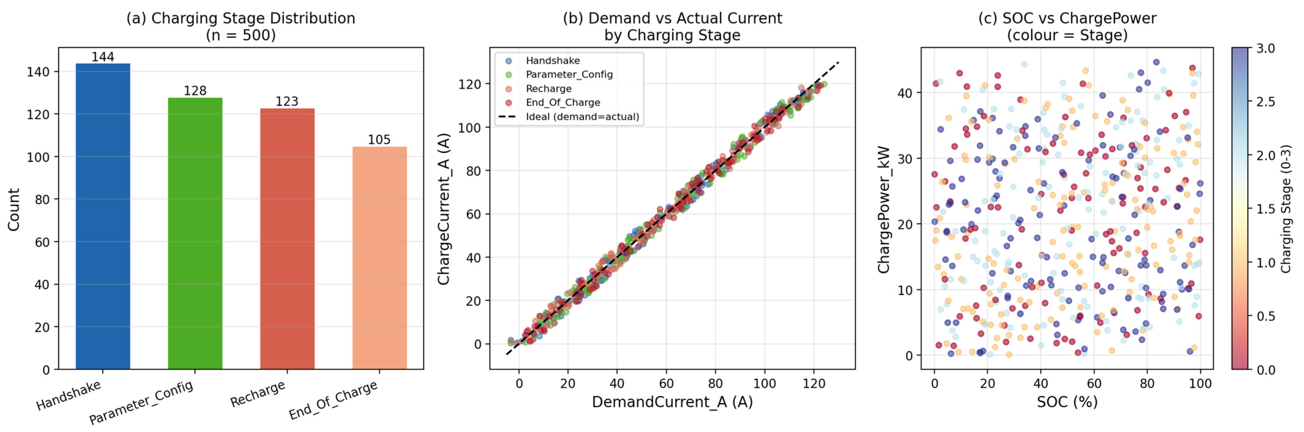
The dataset used in this study is the publicly available EV Battery Charging & Thermal Runaway Dataset [28], released under a CC0 public-domain license. As shown in Figure 1, it contains 500 one-minute lithium-ion battery EV DC-fast-charging records, ten charger identifiers (CH1–CH10), fifty battery-cell identifiers (CELL1–CELL50), and timestamps. The timestamps form a chronological record, but the release does not provide explicit charging-session delimiters. The revised analysis, therefore, uses charger-grouped validation to test identifier-disjoint generalization; it does not claim session-disjoint validation.

The Handshake stage contains 144 samples, representing 28.8% of the dataset, and corresponds to the initial charger–BMS communication and connection-verification process. The Parameter Configuration stage contains 128 samples, representing 25.6%, and describes the period in which charging capability, voltage limits, current limits, and battery readiness are aligned. The Recharge stage contains 123 samples, representing 24.6%, and corresponds to the main energy-transfer phase. The End of Charge stage contains 105 samples, representing 21.0%, and captures the tapering or saturation region near charge completion. The absence of a separate constant-current charging stage indicates that the dataset is more strongly focused on protocol transitions and delivered-response estimation than on long-duration steady-state bulk charging.

2.2. Protocol Variables and Target Definitions

Table 1. The input features and regression targets used in the dual-output estimation framework.

Variable	Type	Unit	Role in Parameter Estimation
Encoded charging stage	Input	-	Protocol-phase context represented as an ordinal stage variable
${\mathrm{D}\mathrm{e}\mathrm{m}\mathrm{a}\mathrm{n}\mathrm{d}\mathrm{V}\mathrm{o}\mathrm{l}\mathrm{t}\mathrm{a}\mathrm{g}\mathrm{e}}_{\mathrm{V}}$	Input	V	Charger-requested voltage setpoint during protocol negotiation
${\mathrm{D}\mathrm{e}\mathrm{m}\mathrm{a}\mathrm{n}\mathrm{d}\mathrm{C}\mathrm{u}\mathrm{r}\mathrm{r}\mathrm{e}\mathrm{n}\mathrm{t}}_{\mathrm{A}}$	Input	A	Charger-requested current setpoint during protocol negotiation
${\mathrm{P}\mathrm{a}\mathrm{c}\mathrm{k}\mathrm{V}\mathrm{o}\mathrm{l}\mathrm{t}\mathrm{a}\mathrm{g}\mathrm{e}}_{\mathrm{V}}$	Input	V	Measured battery-pack terminal voltage at the sampling instant
${\mathrm{C}\mathrm{e}\mathrm{l}\mathrm{l}\mathrm{V}\mathrm{o}\mathrm{l}\mathrm{t}\mathrm{a}\mathrm{g}\mathrm{e}}_{\mathrm{V}}$	Input	V	Cell-level voltage indicator linked to voltage-limit and tapering behavior
${\mathrm{S}\mathrm{O}\mathrm{C}}_{\%}$	Input	%	State-of-charge indicator governing current acceptance and tapering
Maximum temperature	Input	°C	Thermal-condition signal associated with derating and safety constraints
Internal resistance	Input	mΩ	Electrical impedance indicator affecting voltage drop and delivered power
State of health	Input	%	Aging-state indicator affecting charge acceptance and battery response
Ambient temperature	Input	°C	External thermal boundary condition influencing battery thermal behavior
${\mathrm{C}\mathrm{h}\mathrm{a}\mathrm{r}\mathrm{g}\mathrm{e}\mathrm{P}\mathrm{o}\mathrm{w}\mathrm{e}\mathrm{r}}_{\mathrm{k}\mathrm{W}}$	Target 1	kW	Realized delivered charging power
${\mathrm{C}\mathrm{h}\mathrm{a}\mathrm{r}\mathrm{g}\mathrm{e}\mathrm{C}\mathrm{u}\mathrm{r}\mathrm{r}\mathrm{e}\mathrm{n}\mathrm{t}}_{\mathrm{A}}$	Target 2	A	Realized delivered charging current

defines the ten input features and two regression targets used in the proposed dual-output estimation framework. The selected inputs represent the information that would be available to a predictive charging controller during protocol negotiation and power delivery. These include the charging-stage context, demanded electrical setpoints, measured pack state, and battery-condition variables. The two targets represent the realized outputs that the proposed model estimates simultaneously.

The first target, ${\mathrm{C}\mathrm{h}\mathrm{a}\mathrm{r}\mathrm{g}\mathrm{e}\mathrm{P}\mathrm{o}\mathrm{w}\mathrm{e}\mathrm{r}}_{\mathrm{k}\mathrm{W}}$, is the instantaneous electrical power delivered to the battery pack. It is the main variable required for energy-balance calculation, thermal-management scheduling, and high-power event detection. The second target, ${\mathrm{C}\mathrm{h}\mathrm{a}\mathrm{r}\mathrm{g}\mathrm{e}\mathrm{C}\mathrm{u}\mathrm{r}\mathrm{r}\mathrm{e}\mathrm{n}\mathrm{t}}_{\mathrm{A}}$, is the delivered battery-pack current. This variable is directly linked to the lithium-ion intercalation rate, Joule heating, current tapering, and electrochemical aging behavior. Modeling the two targets jointly is technically appropriate because delivered power and delivered current are physically coupled through pack voltage.

2.3. Descriptive Statistics by Charging Stage

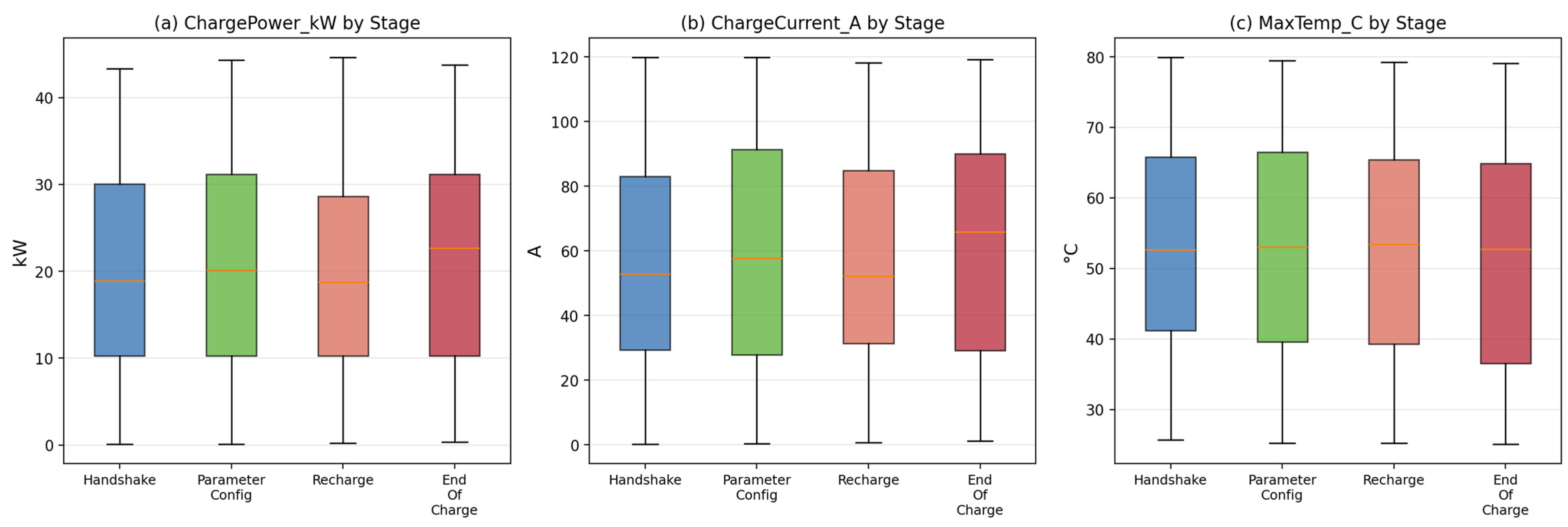
The distribution of the target variables across charging stages is important because the same demanded voltage and current may produce different delivered outputs depending on the protocol state and battery condition (see Figure 2).

Table 2. Output-variable statistics by charging stage.

Stage	$\mathit{n}$	Mean $\mathit{P}$ (kW)	SD $\mathit{P}$ (kW)	Mean $\mathit{I}$ (A)	SD $\mathit{I}$ (A)	Mean Maximum Temperature (°C)
Handshake	144	20.03	12.14	43.2	24.5	52.1
Parameter Configuration	128	20.98	11.89	45.8	23.9	53.4
Recharge	123	19.35	11.24	46.0	25.0	53.2
End of Charge	105	21.37	13.30	44.9	26.1	53.2
Overall	500	20.39	11.84	44.9	24.9	52.8

summarizes the stage-wise descriptive statistics for delivered charging power, delivered charging current, and maximum temperature. The overall mean charging power is 20.39 kW, with a standard deviation of 11.84 kW, while the overall mean charging current is 44.9 A, with a standard deviation of 24.9 A. These values indicate that the dataset contains substantial operating variability, which is necessary for evaluating nonlinear prediction models.

The End of Charge stage exhibits the highest mean delivered power at 21.37 kW and also the largest power variability, with a standard deviation of 13.30 kW. This is consistent with the non-uniform electrical behavior expected near the tapering and saturation region, where the charging process may experience rapid changes in current acceptance and voltage regulation. The Parameter Configuration stage shows the highest mean maximum temperature at 53.4 °C and a relatively high mean current of 45.8 A, indicating that the negotiation stage contains important information about the subsequent delivered response.

The Recharge stage has the lowest mean delivered power among the four stages, at 19.35 kW, but maintains the highest mean charging current, at 46.0 A. These stage-dependent differences justify the inclusion of encoded charging stage as a context variable in the proposed model.

2.4. The State-of-the-Art in EV Fast-Charging Parameter Estimation

EV fast-charging research has progressed from infrastructure-level studies toward more intelligent, data-driven models for charging prediction, control, and battery system management. The technical foundation of this area is defined by fast DC charging infrastructure, charging standards, and charger–vehicle communication protocols. Reviews of fast DC charging infrastructure emphasize that high-power charging requires coordinated management of charger capability, connector standards, converter operation, and battery safety limits [4]. Broader reviews of EV charging systems further show that charging performance depends not only on the charger topology but also on the interaction between the charger, the battery pack, the BMS, and the grid-side interface [5]. Recent work on charging standards and sustainable transportation technologies also confirms that interoperability and protocol-level coordination remain central challenges in practical EV fast-charging deployment [6].

Power-electronics studies provide the physical basis for understanding the demand––delivery gap in fast charging. Charger-topology reviews show that delivered current and delivered power are constrained by converter architecture, charging power level, efficiency, and protection limits [14]. Studies on modern charging systems further indicate that high-power charging requires careful control of voltage and current delivery to prevent excessive stress on the battery and converter hardware [11]. These findings support the need for a data-driven forward model that estimates the realized charging response rather than assuming that demanded setpoints are always achieved exactly.

Battery thermal management and aging studies establish the physical importance of predicting delivered charging power and current. Longevity-conscious power-management research shows that the battery operating strategy has a direct effect on lifetime and performance degradation [15]. Reviews of phase-change-material-based thermal management demonstrate that temperature regulation is critical for maintaining lithium-ion battery safety during high-power operation [16]. Similarly, studies on battery thermal management in hybrid and electric vehicles confirm that heat generation and temperature rise are closely linked to current flow, internal resistance, and operating condition [17]. Low-temperature EV studies further show that battery performance, charging acceptance, and grid impacts vary significantly with environmental and thermal conditions [18]. These studies justify the inclusion of temperature, internal resistance, the state of charge, and the state of health in the present prediction framework.

Battery modeling and BMS research has also highlighted the importance of estimating state-dependent battery behavior. Observer-based studies for state of charge and state of health show that battery-condition estimation is essential for safe and efficient control [19]. Broader reviews of battery modeling, BMS functions, SOC, SOH, and charge–discharge characteristics further demonstrate that battery response is nonlinear and strongly dependent on electrical and thermal operating variables [20]. This motivates the use of machine learning models that can capture nonlinear relationships between demanded setpoints, measured battery states, and realized charging outputs. However, many existing models focus on SOC estimation, SOH estimation, thermal prediction, or charging-demand forecasting rather than the simultaneous estimation of delivered charging power and delivered charging current.

Machine learning has become increasingly important in EV charging analytics because it can model complex charging behavior without requiring a complete first-principles electrochemical representation. Existing learning-based studies have demonstrated the value of predictive models for charging-system intelligence and battery management [24]. Other data-driven battery and charging studies show that machine learning can improve prediction accuracy when nonlinear operating relationships are present [25]. Nevertheless, gradient-trained neural networks may suffer from sensitivity to initialization, local minima, and limited generalization when datasets are moderate in size and outputs have different numerical scales [26]. These issues are particularly relevant for the present dataset, where the model must learn two coupled outputs from only 500 samples.

Metaheuristic optimization offers an alternative learning route by optimizing the neural-network weight vector directly. Prior HPWOA-based research has shown that combining PSO and WOA can improve convergence compared with standalone PSO, WOA, and SFSA in battery-related prediction and feature-selection tasks [27]. However, the application of the HPWOA to dual-output EV fast-charging parameter estimation remains insufficiently explored. In particular, the existing literature does not provide a controlled comparison in which PSO, the WOA, the SFSA, and the HPWOA are evaluated under the same dataset, neural architecture, output targets, and fitness function. This creates a methodological gap that the present study addresses by using a shared dual-output feedforward neural network and a combined MSE objective for simultaneous ${\mathrm{C}\mathrm{h}\mathrm{a}\mathrm{r}\mathrm{g}\mathrm{e}\mathrm{P}\mathrm{o}\mathrm{w}\mathrm{e}\mathrm{r}}_{\mathrm{k}\mathrm{W}}$ and ${\mathrm{C}\mathrm{h}\mathrm{a}\mathrm{r}\mathrm{g}\mathrm{e}\mathrm{C}\mathrm{u}\mathrm{r}\mathrm{r}\mathrm{e}\mathrm{n}\mathrm{t}}_{\mathrm{A}}$ estimation. The positioning of the existing literature and the proposed study is summarized in

Table 3. Positioning of existing work and proposed study.

Category	Ref.	Focus	Strengths	Remaining Limitation
Fast-charging infrastructure and standards	[4,5]	DC fast-charging systems, charging interfaces, and infrastructure requirements	Establishes the technical and operational context for EV fast charging	Does not estimate realized charging power and current at the protocol level
Charging standards and interoperability	[6]	EV charging standards and sustainable charging technologies	Highlights protocol coordination and charger–vehicle compatibility	Does not provide a data-driven demand–delivery prediction model
Charger topology and power electronics	[11,14]	Battery-charger architectures, power levels, and converter constraints	Explains why the demanded and delivered charging quantities may differ	Mainly hardware-focused; limited learning-based estimation
Battery thermal management	[16,17]	Thermal control, heat generation, and battery-pack temperature management	Provides physical motivation for predicting high-power and high-current events	Requires an accurate forward estimate of charging power and current
Battery lifetime and operating-condition effects	[15,18]	Battery longevity, low-temperature operation, and charging acceptance	Links charging conditions to battery performance and degradation	Does not directly model protocol-stage-dependent delivered outputs
BMS and battery-state modeling	[19,20]	SOC, SOH, BMS functions, and charge-discharge characteristics	Establishes the nonlinear relationship between battery state and charging response	Often focused on state estimation rather than dual-output charging-parameter estimation
Machine-learning-based charging prediction	[24,25]	Data-driven modeling of nonlinear charging and battery behavior	Captures nonlinear relationships without full electrochemical models	Often single-output or demand-level prediction; limited protocol-level modeling
Neural-network optimization challenges	[26]	Non-convex learning and optimization difficulty in neural models	Justifies the need for robust optimization strategies	Gradient-based learning may be sensitive to local minima and initialization
HPWOA-based battery intelligence	[27]	Hybrid PSO-WOA optimization for battery-related prediction and feature selection	Provides strong convergence and benchmark performance against standalone algorithms	Not previously formulated for dual-output EV fast-charging power and current estimation
Proposed study	-	HPWOA-optimized dual-output neural framework for estimating ${\mathrm{C}\mathrm{h}\mathrm{a}\mathrm{r}\mathrm{g}\mathrm{e}\mathrm{P}\mathrm{o}\mathrm{w}\mathrm{e}\mathrm{r}}_{\mathrm{k}\mathrm{W}}$ and ${\mathrm{C}\mathrm{h}\mathrm{a}\mathrm{r}\mathrm{g}\mathrm{e}\mathrm{C}\mathrm{u}\mathrm{r}\mathrm{r}\mathrm{e}\mathrm{n}\mathrm{t}}_{\mathrm{A}}$	Uses one shared model, one combined MSE fitness function, and controlled benchmarking against PSO, WOA, and SFSA	Dataset size is moderate and should be expanded in future real-world charging deployments

.

Related intelligent-EV studies demonstrate complementary control-oriented paths. Tian et al. [29] use dynamic state prediction to support pre-stability control in an in-wheel-motor EV, whereas Zhang et al. [30] combine model-based and data-driven components for adaptive clamping-force estimation in an electromechanical brake. These studies do not estimate fast-charging power or current, but they establish two relevant methodological precedents: reconstructing difficult-to-measure quantities and incorporating predicted states into proactive control. In the present study, the direct estimates are, therefore, positioned as indicators for future charging supervision rather than as a deployed controller.

This gap is important because EV fast-charging control is not only a charging-demand forecasting problem. It is also a protocol-aware estimation problem in which the charger-requested setpoints must be translated into actual delivered battery-pack quantities under stage-dependent, electrical, and thermal constraints. Under these conditions, the relative advantage of a hybrid metaheuristic optimizer over standalone search algorithms cannot be assumed; it must be tested under identical model and dataset conditions. The present study, therefore, introduces a controlled HPWOA-based dual-output estimation framework in which the same neural architecture, same input feature space, same training-testing split, and same regression metrics are used to evaluate the HPWOA, PSO, WOA, and SFSA.

3. Materials and Methods

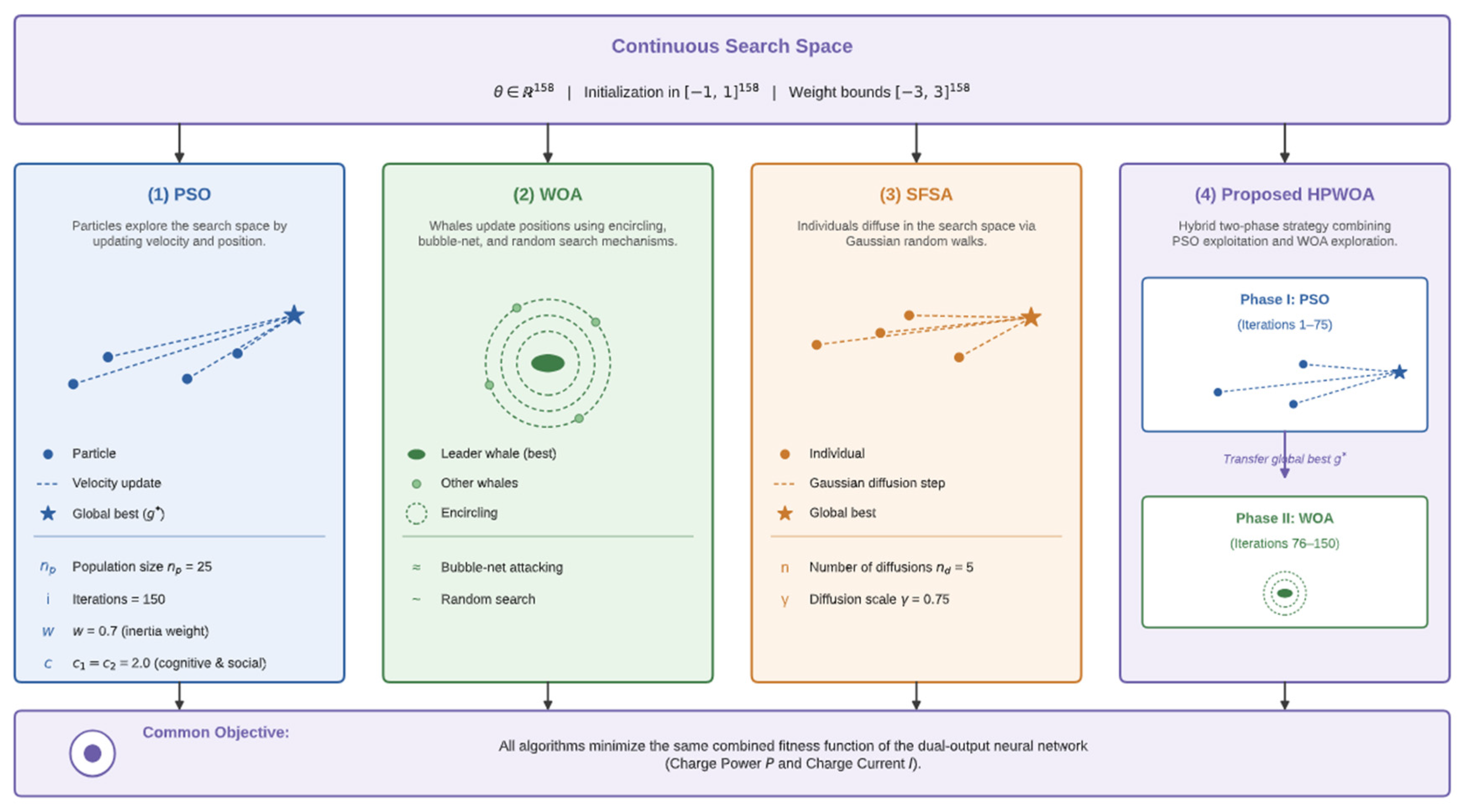
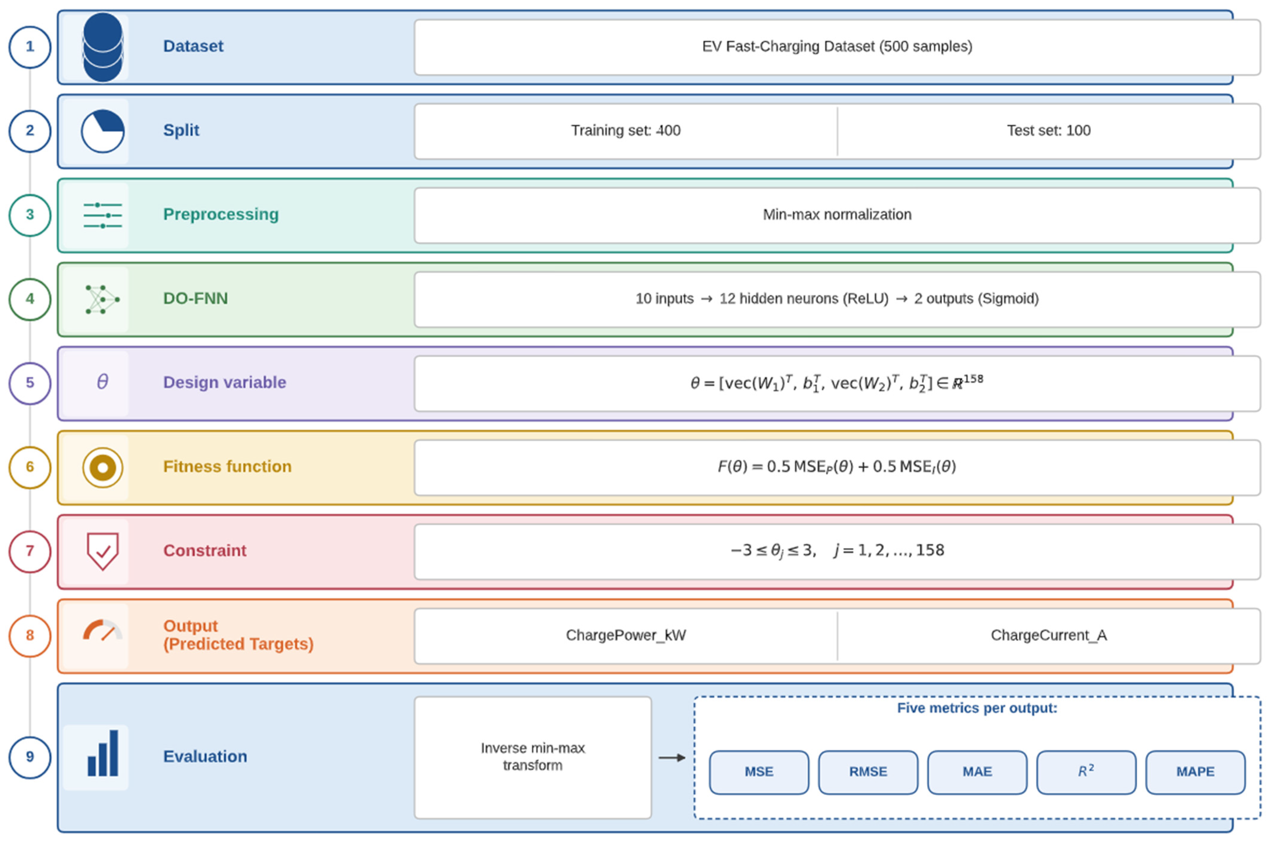
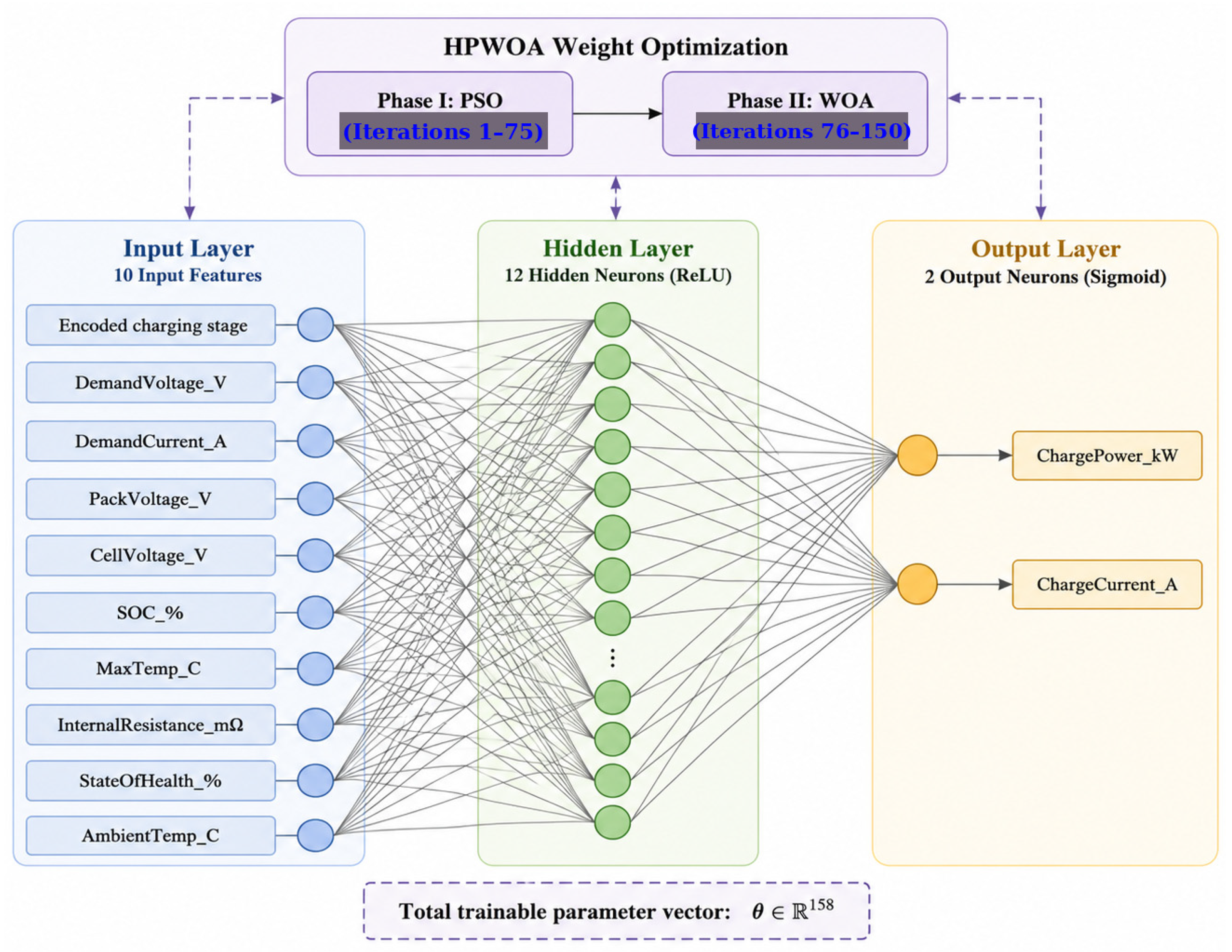
To improve methodological clarity and reproducibility, the proposed HPWOA-based dual-output estimation framework is organized as a structured workflow consisting of data partitioning, normalization, dual-output neural-network modeling, metaheuristic weight optimization, fitness evaluation, and test-set performance assessment. This sequential structure ensures that each stage of the proposed framework is logically connected and that the same experimental conditions are maintained across the proposed HPWOA and the benchmark algorithms. The proposed method estimates two physically coupled EV fast-charging outputs, namely the delivered charging power and the delivered charging current, from the same protocol-state and battery-condition feature space. Figure 3 shows the dual-output feedforward neural network optimized by the proposed HPWOA strategy. Figure 4 illustrates the benchmark optimization algorithms and the two-phase HPWOA search mechanism. Figure 5 summarizes the full problem formulation and evaluation pipeline, from the original EV fast-charging dataset to the final regression metrics.

3.1. Data Partitioning and Normalization

The complete dataset contains $N=500$ EV fast-charging samples. The dataset is divided into a training set and a held-out test set. The training set contains $N_{\mathrm{t}\mathrm{r}}=400$ samples, while the test set contains $N_{\mathrm{t}\mathrm{e}}=100$ samples. The training set is used to optimize the neural-network weight vector, while the test set is used only for final performance evaluation. Let the input matrix be defined as shown in Equaton (1).

The revised sample-level evaluation uses a reproducible 80/20 split (400 training records and 100 held-out test records), stratified by charging stage with random state 42. Min–max scaling parameters are fitted on the training records and then applied to the test records. Because charger and cell identifiers can occur in both partitions, this split is a within-dataset estimate only. Section 4.12 additionally reports five-fold charger-grouped validation, for which every test charger is absent from the corresponding training fold.

$$X=\left[\begin{array}{cccc}{x}_{\mathrm{1,1}}& x_{\mathrm{1,2}}& \dots & x_{\mathrm{1,10}}\\ x_{\mathrm{2,1}}& x_{\mathrm{2,2}}& \dots & x_{\mathrm{2,10}}\\ ⋮& ⋮& \ddots & ⋮\\ x_{N,1}& x_{N,2}& \dots & x_{N,10}\end{array}\right]\in {\mathbb{R}}^{N\times 10},$$

(1)

where each row represents one EV fast-charging snapshot, and each column represents one input feature. The corresponding dual-output target matrix is

$$Y=\left[\begin{array}{cc}{y}_{P,1}& y_{I,1}\\ y_{P,2}& y_{I,2}\\ ⋮& ⋮\\ y_{P,N}& y_{I,N}\end{array}\right]\in {\mathbb{R}}^{N\times 2},$$

(2)

where $y_{P,k}$ denotes the measured charging-power target and $y_{I,k}$ denotes the measured charging-current target for sample $k$. Before training, all input and output variables are scaled using min–max normalization to ensure numerical stability during sigmoid-based output prediction. For a generic variable $z$, the normalized value $z^{\mathrm{n}\mathrm{o}\mathrm{r}\mathrm{m}}$ is computed as

$$z^{\mathrm{n}\mathrm{o}\mathrm{r}\mathrm{m}}={\displaystyle \frac{z-z_{\mathrm{m}\mathrm{i}\mathrm{n}}}{z_{\mathrm{m}\mathrm{a}\mathrm{x}}-z_{\mathrm{m}\mathrm{i}\mathrm{n}}}},$$

(3)

where $z_{\mathrm{m}\mathrm{i}\mathrm{n}}$ and $z_{\mathrm{m}\mathrm{a}\mathrm{x}}$ are computed from the training set. The same training-set normalization parameters are then applied to the test set to prevent information leakage.

3.2. Dual-Output Feedforward Neural Network Architecture

The prediction model is a compact dual-output feedforward neural network (DO-FNN). The architecture contains ten input neurons, twelve hidden neurons with rectified linear unit (ReLU) activation, and two output neurons with sigmoid activation. The two output neurons simultaneously estimate the normalized charging power and normalized charging current. Let $N_{\mathrm{i}\mathrm{n}}=10$, $N_h=12$, and $N_{\mathrm{o}\mathrm{u}\mathrm{t}}=2$ denote the number of input, hidden, and output neurons, respectively. The complete trainable parameter vector is written as

$$\theta ={\left[\mathrm{v}\mathrm{e}\mathrm{c}(W_1{)}^T,b_1^T,\mathrm{v}\mathrm{e}\mathrm{c}(W_2{)}^T,b_2^T\right]}^T,$$

(4)

where $W_1\in {\mathbb{R}}^{10\times 12}$ is the input-to-hidden weight matrix, $b_1\in {\mathbb{R}}^{12}$ is the hidden-layer bias vector, $W_2\in {\mathbb{R}}^{12\times 2}$ is the hidden-to-output weight matrix, and $b_2\in {\mathbb{R}}^2$ is the output-layer bias vector. The total number of trainable parameters is

$$D=(N_{\mathrm{i}\mathrm{n}}\times N_h)+N_h+(N_h\times N_{\mathrm{o}\mathrm{u}\mathrm{t}})+N_{\mathrm{o}\mathrm{u}\mathrm{t}},$$

(5)

which gives

$$D=(10\times 12)+12+(12\times 2)+2=120+12+24+2=158.$$

(6)

Therefore, the optimization problem is defined over a continuous 158-dimensional search space:

$$\theta \in {\mathbb{R}}^{158}.$$

(7)

For an input matrix $X$, the hidden-layer activation is computed as

$$H=\mathrm{R}\mathrm{e}\mathrm{L}\mathrm{U}(X{W}_1+b_1),$$

(8)

where the ReLU activation function is defined as

$$\mathrm{R}\mathrm{e}\mathrm{L}\mathrm{U}\left(u\right)=\mathrm{m}\mathrm{a}\mathrm{x}(0,u).$$

(9)

The output layer is then computed as

$$\widehat{Y}=\left[\begin{array}{cc}{\widehat{y}}_P& {\widehat{y}}_I\end{array}\right]=\sigma (H{W}_2+b_2),$$

(10)

where ${\widehat{y}}_P$ is the normalized predicted charging power, ${\widehat{y}}_I$ is the normalized predicted charging current, and $\sigma (\cdot )$ is the sigmoid activation function:

$$\sigma (u)={\displaystyle \frac{1}{1+e^{-u}}}.$$

(11)

The sigmoid output activation is appropriate because both target variables are min–max normalized to the interval $\left[0,1\right]$. After prediction, the normalized outputs are transformed back into their original physical units using inverse min-max transformation.

3.3. Continuous Search Space and Optimization Constraints

All optimization algorithms operate on the same continuous neural-network weight vector and use the same network architecture, 400-record training partition, objective, and population size (n_p = 25). For the repeated comparison, PSO, the WOA, and the HPWOA run for 150 iterations (25 initial candidates plus 25 × 150 = 3775 fitness-function evaluations (FFEs)); SFSA runs for 30 iterations because its five diffusion candidates per individual yield the same 25 + 25 × 5 × 30 = 3775 FFEs. This comparison is FFE-matched. Adam is reported as a separate gradient-based benchmark because its mini-batch updates are not directly equivalent to black-box FFEs.

$${\theta }_j^{\left(0\right)}\sim \mathcal{U}(-\mathrm{1,1}),j=\mathrm{1,2},\dots ,158.$$

(12)

During the optimization process, all weight components are constrained by

$$-3\le {\theta }_j\le 3,j=\mathrm{1,2},\dots ,158.$$

(13)

This constraint prevents extreme weights from causing sigmoid saturation or unstable hidden-layer activations. For PSO-based updates, particle velocities are additionally clipped to

$$-0.5\le v_j\le 0.5,j=\mathrm{1,2},\dots ,158.$$

(14)

3.4. Particle Swarm Optimization

Particle Swarm Optimization (PSO) is included as a standard benchmark and as Phase I of the HPWOA. Each particle encodes the full neural-weight vector; the standard velocity and position updates in Equations (15) and (16) are used without modification.

$$v_i^{t+1}=w{v}_i^t+c_1{r}_1\left(p_i^t−{\theta }_i^t\right)+c_2{r}_2\left(g^t−{\theta }_i^t\right),$$

(15)

Equation (15) uses the standard inertia, cognitive, and social terms. The standalone PSO benchmark runs for 150 iterations; the HPWOA uses this unmodified update only for iterations 1–75.

$${\theta }_i^{t+1}={\theta }_i^t+v_i^{t+1}.$$

(16)

In this study, PSO uses a population size of $n_p=25$, inertia weight $w=0.7$, and acceleration coefficients $c_1=c_2=2.0$. For the standalone PSO benchmark, the algorithm runs for 150 iterations. For the HPWOA, PSO is used only during Phase I, corresponding to iterations 1–75.

3.5. Whale Optimization Algorithm

The Whale Optimization Algorithm (WOA) is included as a standard benchmark and as Phase II of the HPWOA. The unmodified encircling, spiral bubble-net, and random-search rules are retained in Equations (17)–(23).

$$A=2ar-a,$$

(17)

$$C=2r,$$

(18)

$$D_i=\mid C\cdot g^t-{\theta }_i^t\mid ,$$

(19)

$${\theta }_i^{t+1}=g^t-A\cdot D_i,$$

(20)

The leader and control parameters follow the standard WOA formulation; the only hybrid-specific choice is the population hand-off after the PSO phase.

$$D_i^{\prime }=\mid g^t-{\theta }_i^t\mid ,$$

(21)

$${\theta }_i^{t+1}=D_i^{\prime }{e}^{bl}\mathrm{c}\mathrm{o}\mathrm{s}\left(2\pi l\right)+g^t,$$

(22)

where $b=1$ is the spiral-shape constant and $l\in [-\mathrm{1,1}]$ is a random number. If $\mid A\mid \ge 1$, the WOA performs random prey search using a randomly selected whale ${\theta }_{\mathrm{r}\mathrm{a}\mathrm{n}\mathrm{d}}^t$:

$$D_i^{\mathrm{r}\mathrm{a}\mathrm{n}\mathrm{d}}=\mid C\cdot {\theta }_{\mathrm{r}\mathrm{a}\mathrm{n}\mathrm{d}}^t-{\theta }_i^t\mid ,$$

(23)

$${\theta }_i^{t+1}={\theta }_{\mathrm{r}\mathrm{a}\mathrm{n}\mathrm{d}}^t-A\cdot D_i^{\mathrm{r}\mathrm{a}\mathrm{n}\mathrm{d}}.$$

(24)

The WOA leader is updated whenever a candidate produces a lower combined MSE fitness value than the current best solution.

3.6. Stochastic Fractal Search Algorithm

The Stochastic Fractal Search Algorithm (SFSA) is retained only as a benchmark. Its Gaussian-diffusion update in Equation (24) is used as specified; five diffusion candidates are evaluated per individual and iteration.

$${\theta }_{i,d}^{t+1}={\theta }_i^t+\gamma \hspace{0.17em}\mathcal{N}\left(\mathrm{0,1}\right)\left(g^t−{\theta }_i^t\right),$$

(25)

Equation (24) gives the standard SFSA diffusion step. The resulting extra candidate evaluations are explicitly accounted for in Section 4.12.

3.7. Proposed HPWOA Training Strategy

The HPWOA applies a fixed two-phase schedule: PSO is run in iterations 1–75 and the WOA in iterations 76–150. The 75/75 allocation was a pre-specified equal allocation of the 150-iteration budget; it was not selected using a tuning sweep or an ablation among alternative hybrid schedules. At the hand-off, the complete terminal PSO population is transferred to initialize the WOA population, and the best terminal PSO member initializes the WOA leader. This preserves the terminal population diversity rather than transferring only one leader.

$$g_{\mathrm{W}\mathrm{O}\mathrm{A}}^0=g_{\mathrm{P}\mathrm{S}\mathrm{O}}^{*}.$$

(26)

The complete HPWOA training strategy is defined as θ* = WOA(PSO(θ; iterations 1–75); iterations 76–150).

$${\theta }^{*}={\mathrm{W}\mathrm{O}\mathrm{A}}_{51:100}\left({\mathrm{P}\mathrm{S}\mathrm{O}}_{1:50}\left(\theta \right)\right),$$

(27)

This schedule makes a testable study-specific design choice: an early PSO search is followed by WOA refinement from the terminal PSO population. The repeated results in Section 4 show that it does not establish superiority over standalone PSO or gradient-based neural-network training under the evaluated settings.

Table 4. The control parameters and fitness-function-evaluation budgets used in the repeated benchmark.

Algorithm	Parameter	Symbol	Value
PSO/HPWOA Phase I	Population size	$n_p$	25
PSO/HPWOA Phase I	Inertia weight	$w$	0.7
PSO/HPWOA Phase I	Cognitive coefficient	$c_1$	2.0
PSO/HPWOA Phase I	Social coefficient	$c_2$	2.0
PSO/HPWOA Phase I	Velocity bounds	$v_{\mathrm{m}\mathrm{a}\mathrm{x}}$	$\left[-0.5, 0.5\right]$
WOA/HPWOA Phase II	Spiral shape constant	$b$	1
WOA/HPWOA Phase II	Weight bounds	$\theta$	$\left[-3, 3\right]$
SFSA	Diffusion steps per iteration	$n_d$	5
SFSA	Gaussian walk ratio	$\gamma$	0.75
Repeated benchmark	FFE-matched iteration allocation	T	150 (PSO/WOA/HPWOA); 30 (SFSA)
All algorithms	Search-space dimension	$D$	158
HPWOA	Phase split	-	75 PSO/75 WOA

summarizes the algorithm-specific control parameters and fitness-function-evaluation budgets adopted for the repeated benchmark experiments.

3.8. Dual-Output Fitness Function

The optimization objective is to minimize the combined prediction error over both target variables on the training set. Since both outputs are normalized to $\left[0,1\right]$, an equal-weight combined mean-square-error fitness function is used:

$$F\left(\theta \right)=0.5\hspace{0.17em}{\mathrm{M}\mathrm{S}\mathrm{E}}_P\left(\theta \right)+0.5\hspace{0.17em}{\mathrm{M}\mathrm{S}\mathrm{E}}_I\left(\theta \right).$$

(28)

The charging-power MSE is defined as

$${\mathrm{M}\mathrm{S}\mathrm{E}}_P(\theta )={\displaystyle \frac{1}{N_{\mathrm{t}\mathrm{r}}}}{\displaystyle \sum _{k=1}^{N_{\mathrm{t}\mathrm{r}}}}{\left({\widehat{y}}_{P,k}\left(\theta \right)-y_{P,k}\right)}^2,$$

(29)

and the charging-current MSE is defined as

$${\mathrm{M}\mathrm{S}\mathrm{E}}_I(\theta )={\displaystyle \frac{1}{N_{\mathrm{t}\mathrm{r}}}}{\displaystyle \sum _{k=1}^{N_{\mathrm{t}\mathrm{r}}}}{\left({\widehat{y}}_{I,k}\left(\theta \right)-y_{I,k}\right)}^2.$$

(30)

Here, ${\widehat{y}}_{P,k}\left(\theta \right)$ and ${\widehat{y}}_{I,k}\left(\theta \right)$ are the normalized DO-FNN predictions for sample $k$, while $y_{P,k}$ and $y_{I,k}$ are the corresponding normalized ground-truth values. Equal weighting is used because both output variables have the same normalized range and comparable importance in EV fast-charging control.

3.9. Algorithmic Implementation

Algorithm 1 presents the complete HPWOA-based DO-FNN training procedure. The same fitness function is used for all of the algorithms to ensure a fair comparison.

Algorithm 1. HPWOA-based dual-output neural-network training procedure.
Step	Procedure
Input	Training inputs $X_{\mathrm{t}\mathrm{r}},$ training targets $Y_{\mathrm{t}\mathrm{r}},$ population size $n_p=25,$ maximum iterations $N_{\mathrm{i}\mathrm{t}\mathrm{e}\mathrm{r}}=100,$ and neural-network dimension $D=158.$
Output	Optimized weight vector ${\theta }^{*}$ and trained DO-FNN model.
1	Normalize $X_{\mathrm{t}\mathrm{r}}$ and $Y_{\mathrm{t}\mathrm{r}}$ using min–max scaling.
2	Initialize a population of candidate weight vectors: ${\theta }_i^0\sim U\left(-1, 1\right),$ where $i=\mathrm{1,2},\dots ,n_p.$
3	Initialize PSO velocities: $v_i^0\sim U\left(-0.5, 0.5\right).$
4	Evaluate the initial fitness $F\left({\theta }_i^0\right)$ for all particles using Equation (28).
5	Set each personal best as $p_i^0={\theta }_i^0.$
6	Set the global best $g^0$ as the candidate with the lowest fitness.
7	For $t=1$ to $50,$ execute the PSO phase.
7.1	Update particle velocity using Equation (15).
7.2	Clip velocity using Equation (14).
7.3	Update particle position using Equation (16).
7.4	Clip weights using Equation (13).
7.5	Decode ${\theta }_i^t$ into $W_1,$$b_1,$$W_2,$ and $b_2.$
7.6	Compute DO-FNN predictions using Equations (8)–(10).
7.7	Evaluate $F\left({\theta }_i^t\right)$ using Equation (28).
7.8	Update the personal best $p_i^t$ if the current fitness improves.
7.9	Update the global best $g^t$ if the current candidate gives the lowest fitness.
8	Store the complete terminal PSO population $\left\{{\theta }_i^{\left(75\right)}\right\}$ for $i=1,\dots ,n_p$ and its global best $g_{\mathrm{P}\mathrm{S}\mathrm{O}}^{\left(75\right)}.$
9	Initialize the WOA population as $x_i^{\left(76\right)}={\theta }_i^{\left(75\right)}$ for $i=1,\dots ,n_p;$ initialize the WOA leader as $g^{\left(76\right)}=g_{\mathrm{P}\mathrm{S}\mathrm{O}}^{\left(75\right)}.$
10	For $t=76,\dots ,150,$ execute the WOA phase.
10.1	Set the WOA control coefficient $a_t=2-2\left(t-76\right)/\left(150-76\right).$
10.2	For each whale $i,$ draw $p,$$r_1,$$r_2;$ compute $A=2a_t{r}_1-a_t$ and $C=2r_2.$
10.3	If $p<0.5$ and $\left|A\right|<1,$ update $x_i^{\left(t+1\right)}=g^{\left(t\right)}-A\cdot \left|C\cdot g^{\left(t\right)}-x_i^{\left(t\right)}\right|.$
10.4	If $p<0.5$ and $\left|A\right|\ge 1,$ select $x_{\mathrm{r}\mathrm{a}\mathrm{n}\mathrm{d}}$ from the transferred/current WOA population and update $x_i^{\left(t+1\right)}=x_{\mathrm{r}\mathrm{a}\mathrm{n}\mathrm{d}}-A\cdot \left|C\cdot x_{\mathrm{r}\mathrm{a}\mathrm{n}\mathrm{d}}-x_i^{\left(t\right)}\right|.$
10.5	If $p\ge 0.5,$ update the whale using the spiral bubble-net equation in Equations (21) and (22).
10.6	Clip weights using Equation (13).
10.7	Decode each candidate into $W_1,$$b_1,$$W_2,$ and $b_2.$
10.8	Compute DO-FNN predictions using Equations (8)–(10).
10.9	Evaluate the combined fitness using Equation (28).
10.10	Update the leader if a lower fitness value is found.
11	Return the final optimized solution ${\theta }^{*}=g^{100}.$
12	Use ${\theta }^{*}$ to evaluate the trained DO-FNN on the held-out test set.

Algorithm 2 summarizes the evaluation procedure used after optimization.

Algorithm 2. Test-set evaluation procedure.

Input: Test inputs $X_{\mathrm{t}\mathrm{e}}$, test targets $Y_{\mathrm{t}\mathrm{e}}$, and optimized weight vector ${\theta }^{*}$. Output: Test-set MSE, RMSE, MAE, $R^2$, and MAPE for both outputs.   1. Normalize $X_{\mathrm{t}\mathrm{e}}$ using the training-set normalization parameters.   2. Decode ${\theta }^{\mathrm{*}}$ into $W_1$, $b_1$, $W_2$, and $b_2$.   3. Compute normalized predictions:    ${\widehat{Y}}_{\mathrm{t}\mathrm{e}}=\sigma \left(\mathrm{R}\mathrm{e}\mathrm{L}\mathrm{U}\right(X_{\mathrm{t}\mathrm{e}}{W}_1+b_1)W_2+b_2).$   4. Apply inverse min–max transformation to convert predictions back to kW and A.   5. Compute $\mathrm{MSE}, \mathrm{RMSE}, \mathrm{MAE}, R^2$, and MAPE for ${\mathrm{C}\mathrm{h}\mathrm{a}\mathrm{r}\mathrm{g}\mathrm{e}\mathrm{P}\mathrm{o}\mathrm{w}\mathrm{e}\mathrm{r}}_{\mathrm{k}\mathrm{W}}$.   6. Compute $\mathrm{MSE}, \mathrm{RMSE}, \mathrm{MAE}, R^2$, and MAPE for ${\mathrm{C}\mathrm{h}\mathrm{a}\mathrm{r}\mathrm{g}\mathrm{e}\mathrm{C}\mathrm{u}\mathrm{r}\mathrm{r}\mathrm{e}\mathrm{n}\mathrm{t}}_{\mathrm{A}}$.          Report the final test-set metrics for all algorithms.

3.10. Performance Evaluation Metrics

After optimization, all models are evaluated on the held-out test set after inverse min–max transformation to the original physical units. For each output variable $q\in \{P,I\}$, the mean-square error is computed as

$${\mathrm{M}\mathrm{S}\mathrm{E}}_q={\displaystyle \frac{1}{N_{\mathrm{t}\mathrm{e}}}}{\displaystyle \sum _{k=1}^{N_{\mathrm{t}\mathrm{e}}}}{\left(y_{q,k}−{\widehat{y}}_{q,k}\right)}^2.$$

(31)

The root-mean-square error is

$${\mathrm{R}\mathrm{M}\mathrm{S}\mathrm{E}}_q=\sqrt{{\mathrm{M}\mathrm{S}\mathrm{E}}_q}.$$

(32)

The mean absolute error is

$${\mathrm{M}\mathrm{A}\mathrm{E}}_q={\displaystyle \frac{1}{N_{\mathrm{t}\mathrm{e}}}}{\displaystyle \sum _{k=1}^{N_{\mathrm{t}\mathrm{e}}}}\mid y_{q,k}-{\widehat{y}}_{q,k}\mid .$$

(33)

The coefficient of determination is

$$R_q^2=1-{\displaystyle \frac{{\displaystyle {\sum }_{k=1}^{N_{\mathrm{t}\mathrm{e}}}}{\left(y_{q,k}−{\widehat{y}}_{q,k}\right)}^2}{{\displaystyle {\sum }_{k=1}^{N_{\mathrm{t}\mathrm{e}}}}{\left(y_{q,k}−{\overline{y}}_q\right)}^2}}.$$

(34)

The mean absolute percentage error is

$${\mathrm{M}\mathrm{A}\mathrm{P}\mathrm{E}}_q={\displaystyle \frac{100}{N_{\mathrm{t}\mathrm{e}}}}{\displaystyle \sum _{k=1}^{N_{\mathrm{t}\mathrm{e}}}}\mid {\displaystyle \frac{y_{q,k}-{\widehat{y}}_{q,k}}{y_{q,k}}}\mid .$$

(35)

where $y_{q,k}$ is the measured value, ${\widehat{y}}_{q,k}$ is the predicted value, and ${\overline{y}}_q$ is the mean measured value of the output $q$ on the test set. For the charging-power estimation, $q=P$, and the metrics are reported in kW-based units. For the charging-current estimation, $q=I$, and the metrics are reported in ampere-based units. The combined convergence MSE in Equation (28) is used for training-phase comparison, while the five test-set metrics in Equations (31)–(35) are used for final predictive-performance comparison. This separation prevents the training fitness from being confused with the physically interpretable test-set performance.

4. Results and Discussion

This section reports the reproducible 30-seed results for the HPWOA, PSO, WOA, and SFSA on the stated sample-level split, together with a mini-batch Adam DO-FNN benchmark. All metaheuristic runs use the same 3775-FFE budget; Adam is reported separately as a gradient-based baseline. The means, standard deviations, run times, and paired non-parametric tests are used to avoid conclusions from a single stochastic trajectory.

4.1. Convergence Analysis

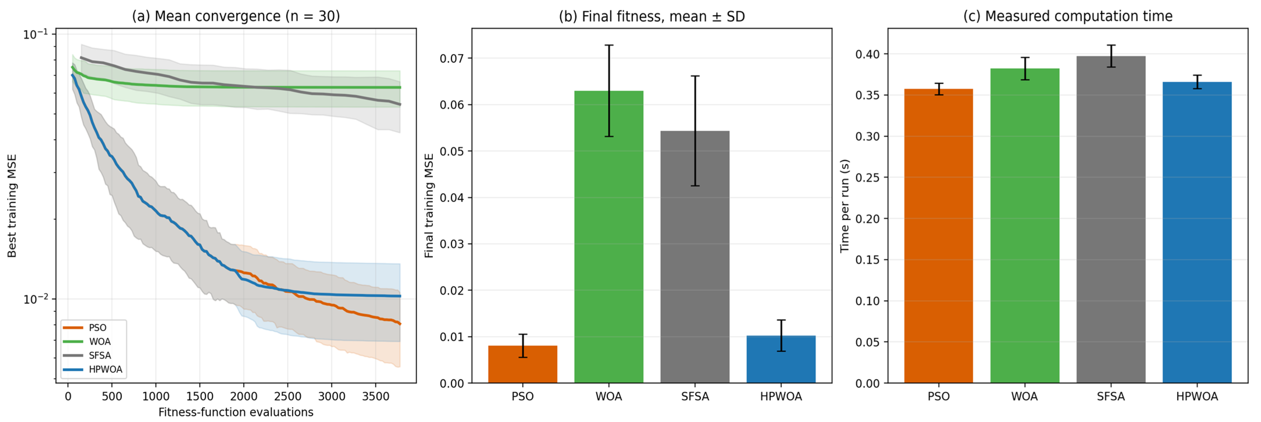
Figure 6 presents the mean convergence over 30 seeds against the common 3775-FFE budget. The final training MSE (mean ± SD) was 0.00807 ± 0.00251 for PSO, 0.06298 ± 0.00984 for the WOA, 0.05436 ± 0.01184 for the SFSA, and 0.01027 ± 0.00334 for the HPWOA. Thus, in the repeated FFE-matched study, standalone PSO had the lowest final training MSE; the HPWOA remained better than the WOA and SFSA but did not improve on PSO.

Table 5. Repeated FFE-matched convergence and computational comparison (mean ± SD across 30 seeds).

Algorithm	Final Training MSE (Mean ± SD)	Convergence Iteration (Mean ± SD)	Time/Run, s (Mean ± SD)
PSO	0.00807 ± 0.00251	138.8 ± 12.3	0.357 ± 0.007
WOA	0.06298 ± 0.00984	38.8 ± 18.7	0.382 ± 0.013
SFSA	0.05436 ± 0.01184	22.5 ± 7.3	0.397 ± 0.013
HPWOA	0.01027 ± 0.00334	115.7 ± 16.1	0.366 ± 0.008

reports the final fitness, convergence iteration, and measured time across the 30 independent seeds. The HPWOA converged in 115.7 ± 16.1 iterations, compared with 138.8 ± 12.3 for PSO; however, the lower final training MSE belonged to PSO. The FFE-matched design removes the original SFSA evaluation-budget advantage. Paired two-sided Wilcoxon tests on the normalized test MSEs show that the HPWOA is worse than PSO (p = 0.00061) and Adam (p < 0.001), but better than the WOA and SFSA (p < 0.001 for each).

4.2. Charging-Power Estimation Performance

Table 6. Sample-level charging-power test metrics (mean ± SD across 30 seeds).

Algorithm	MSE (kW2) (Mean ± SD)	RMSE (kW) (Mean ± SD)	MAE (kW) (Mean ± SD)	R2 (Mean ± SD)
PSO	17.695 ± 6.868	4.133 ± 0.796	3.265 ± 0.606	0.877 ± 0.048
WOA	121.695 ± 29.939	10.943 ± 1.415	9.127 ± 1.401	0.154 ± 0.208
SFSA	111.230 ± 34.689	10.430 ± 1.590	8.268 ± 1.238	0.227 ± 0.241
HPWOA	22.640 ± 10.276	4.658 ± 0.986	3.712 ± 0.799	0.843 ± 0.071
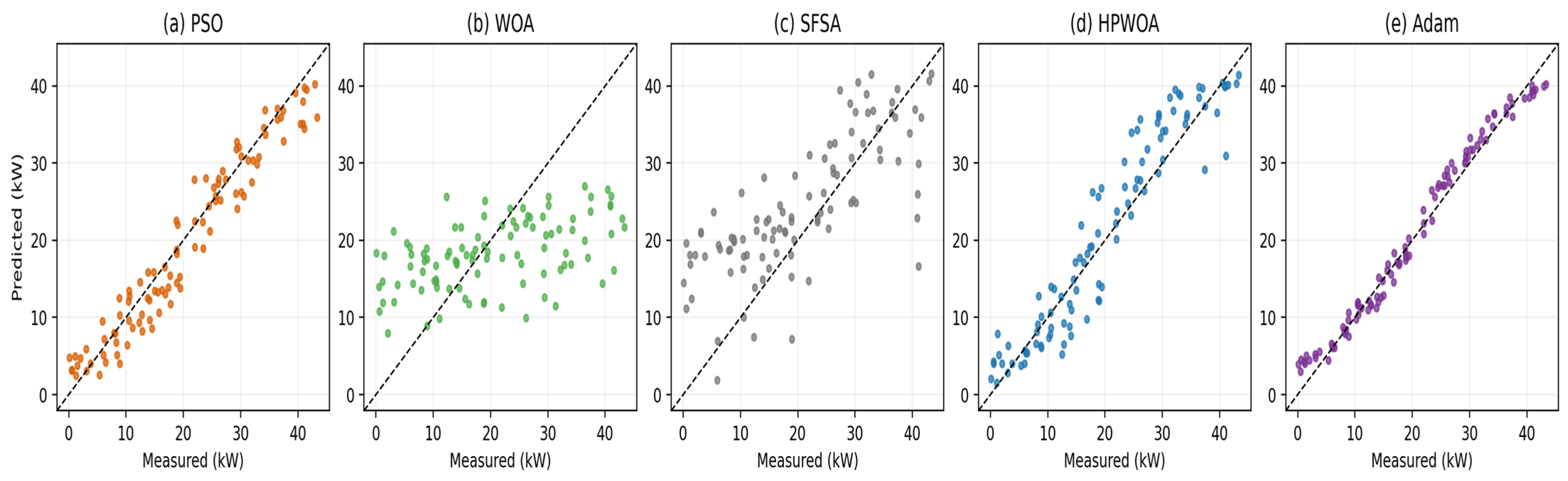
Adam DO-FNN	2.917 ± 0.398	1.704 ± 0.121	1.400 ± 0.099	0.980 ± 0.003

reports the sample-level test performance for charging-power estimation across the 30 seeds. PSO obtained RMSE = 4.133 ± 0.796 kW and R² = 0.877 ± 0.048, compared with the HPWOA at 4.658 ± 0.986 kW and 0.843 ± 0.071. The Adam DO-FNN achieved the lowest power error (RMSE = 1.704 ± 0.121 kW; R² = 0.980 ± 0.003). The HPWOA nevertheless outperformed the WOA and SFSA under the common FFE budget.

Figure 7 visualizes representative runs selected by the median normalized test MSE for each method. The quantitative comparison, including all 30 seeds, is provided in Table 6; the scatter panels are not used for statistical inference.

4.3. Charging-Current Estimation Performance

Table 7. Sample-level charging-current test metrics (mean ± SD across 30 seeds).

Algorithm	MSE (A2) (Mean ± SD)	RMSE (A) (Mean ± SD)	MAE (A) (Mean ± SD)	R2 (Mean ± SD)
PSO	131.139 ± 54.057	11.235 ± 2.255	8.949 ± 1.752	0.889 ± 0.046
WOA	1008.048 ± 231.928	31.507 ± 3.982	26.720 ± 3.845	0.148 ± 0.196
SFSA	813.143 ± 235.903	28.226 ± 4.121	22.532 ± 3.348	0.313 ± 0.199
HPWOA	167.917 ± 70.187	12.686 ± 2.687	10.160 ± 2.073	0.858 ± 0.059
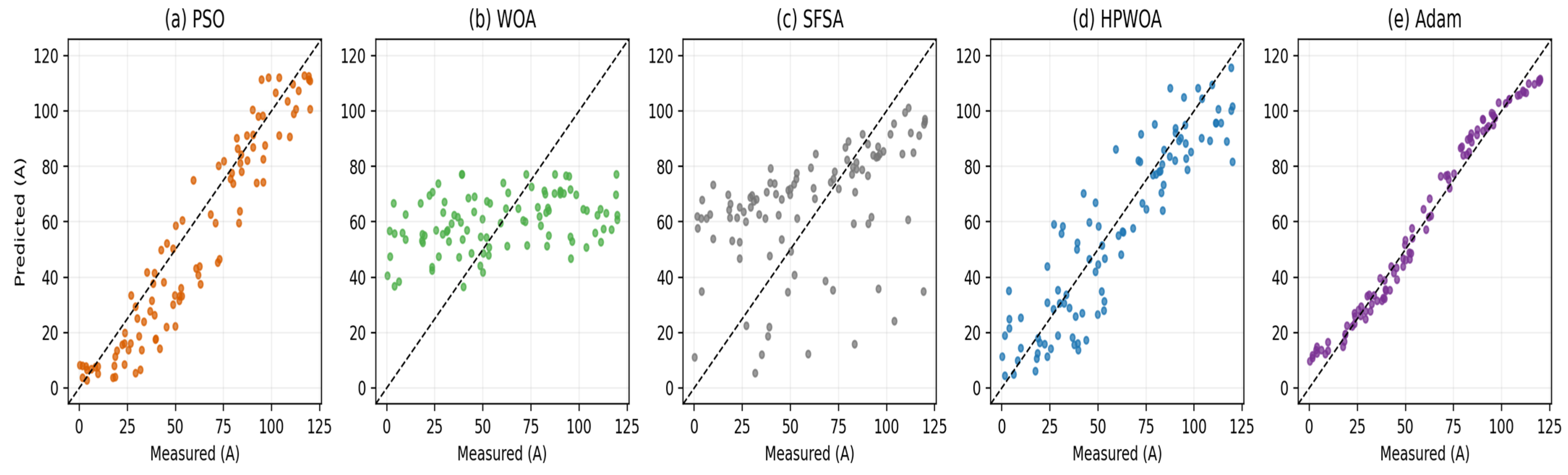
Adam DO-FNN	24.534 ± 2.592	4.946 ± 0.273	4.082 ± 0.221	0.979 ± 0.002

reports sample-level test performance for charging-current estimation across the 30 seeds. PSO obtained RMSE = 11.235 ± 2.255 A and R² = 0.889 ± 0.046, compared with the HPWOA at 12.686 ± 2.687 A and 0.858 ± 0.059. The Adam DO-FNN achieved the lowest current error (RMSE = 4.946 ± 0.273 A; R² = 0.979 ± 0.002). The HPWOA remained better than the WOA and SFSA in this comparison.

Figure 8 visualizes the representative runs selected by the median normalized test MSE for each method. The quantitative comparison, including all 30 seeds, is provided in Table 7; the scatter panels are not used for statistical inference.

4.4. Residual Analysis

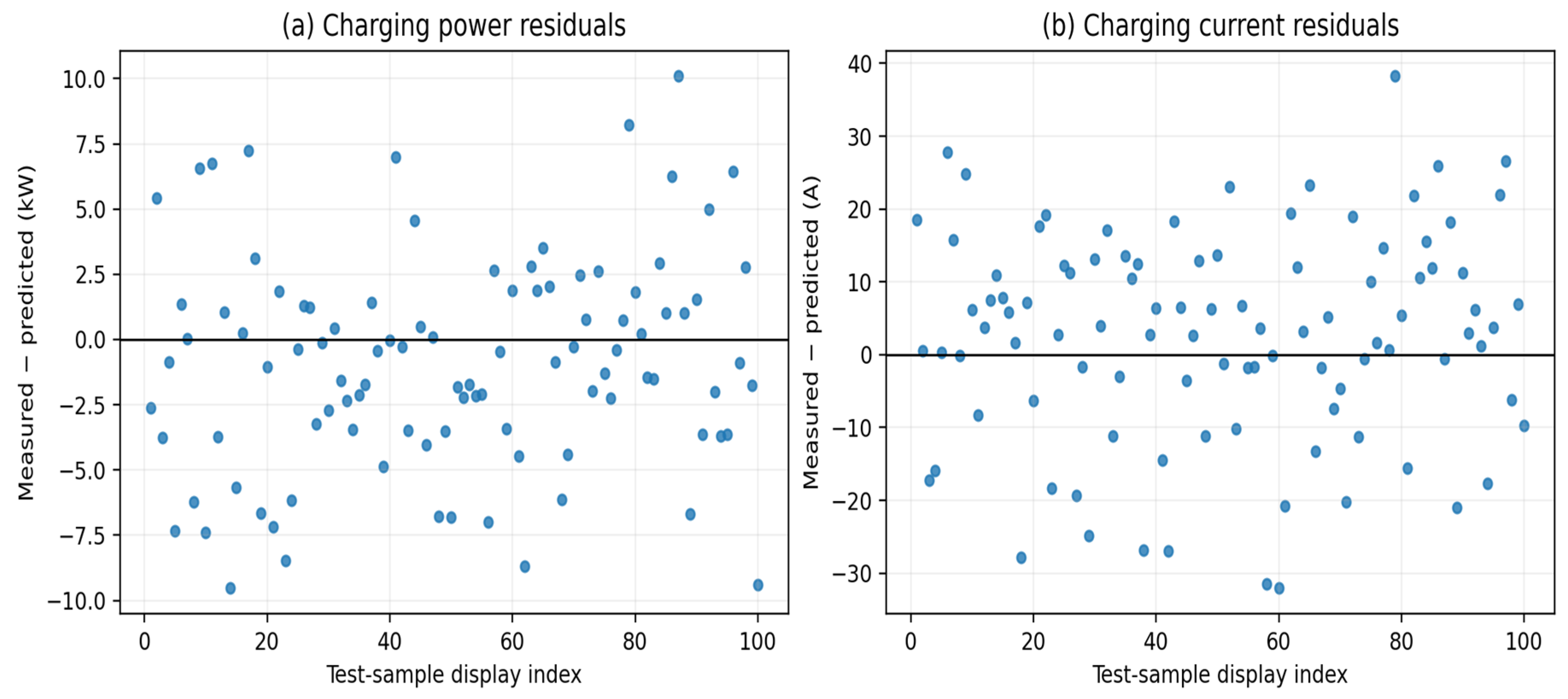
Figure 9 shows residuals for the representative HPWOA run selected by the median normalized test MSE. The plot is descriptive and is included to reveal the scale and distribution of the signed errors across the display-indexed test records; it is not a temporal residual analysis or a formal test of bias.

4.5. Comprehensive Metric Comparison

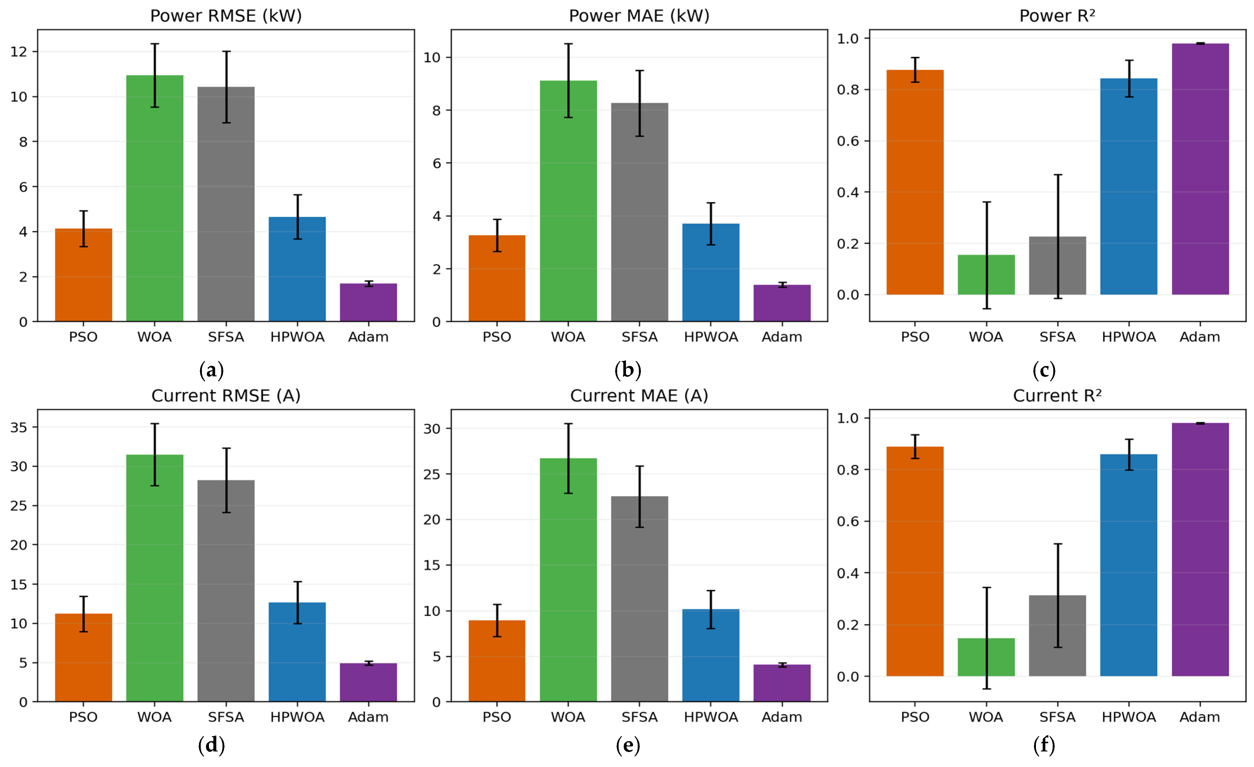
Figure 10 summarizes the mean ± SD regression metrics across the 30 seeds. Adam has the best mean performance for both outputs. Among the metaheuristics, PSO outperforms the HPWOA; the HPWOA outperforms the WOA and SFSA. These replicated results replace the former single-run ranking.

4.6. Ordered Test-Sample Comparison

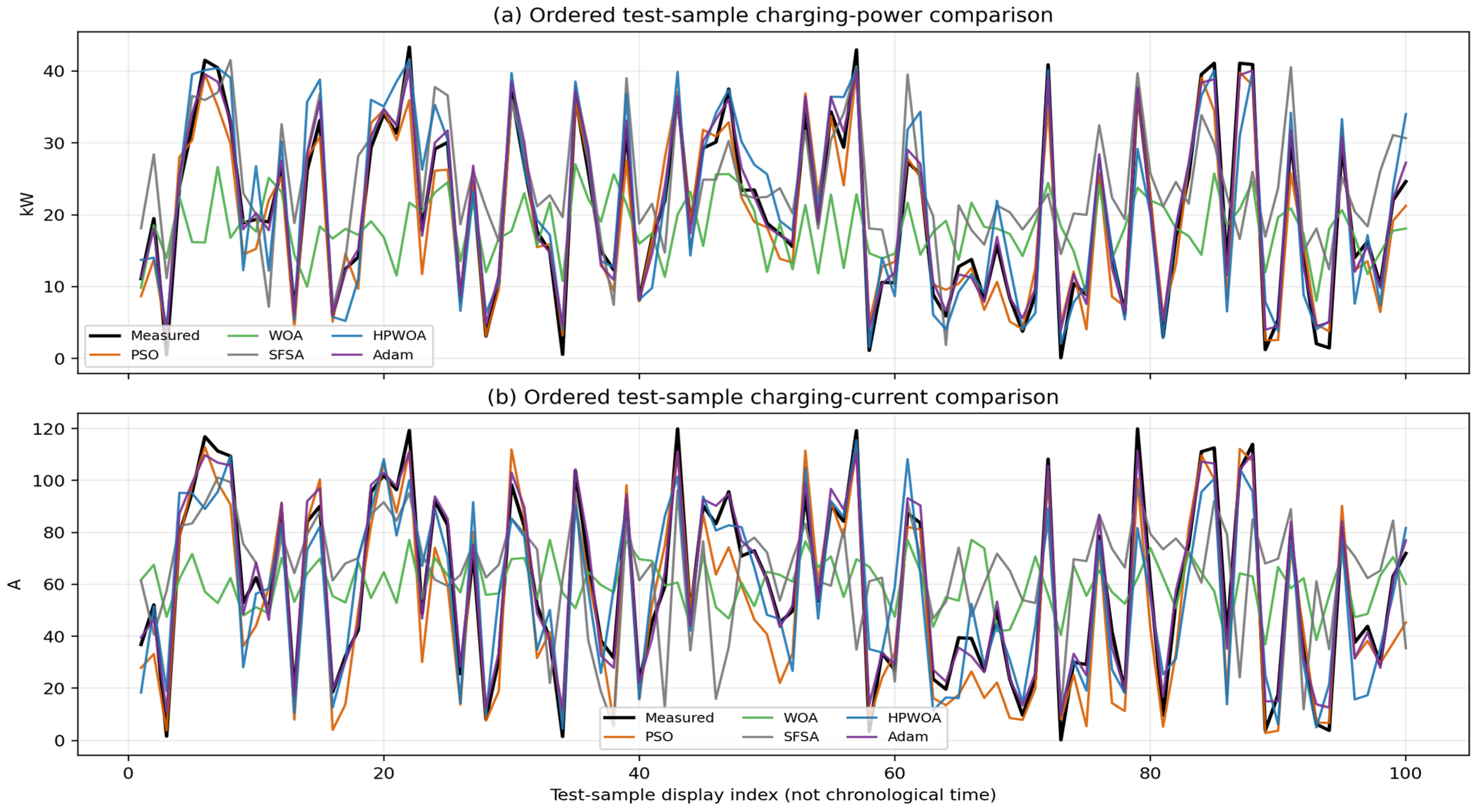
Figure 11 is an ordered-index plot of the 100 held-out samples. The horizontal axis is the post-split display index; it is not a chronological charging-session sequence. The figure, therefore, complements the scatter plots by showing local agreement across the displayed records, but it does not demonstrate temporal forecasting, sequential dependence, or session tracking. It includes the representative PSO, WOA, SFSA, HPWOA, and Adam runs; the corresponding replicated numerical comparisons remain those in Table 6 and Table 7.

4.7. Per-Stage Error Analysis

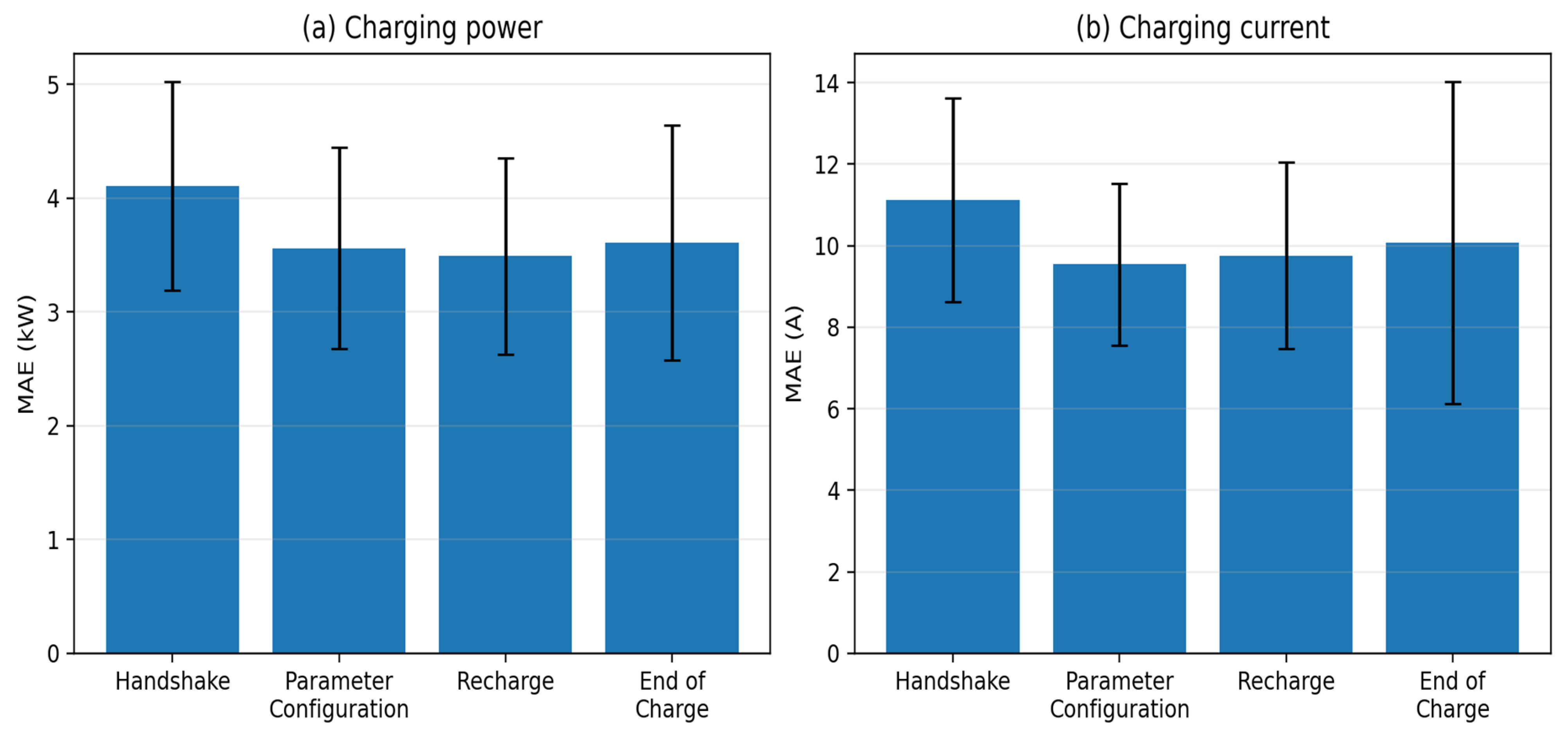
Figure 12 reports the per-stage MAEs averaged across the 30 HPWOA runs. For the charging power, the mean ± SD MAE is 4.107 ± 0.914 kW (Handshake), 3.561 ± 0.883 kW (Parameter Configuration), 3.491 ± 0.865 kW (Recharge), and 3.607 ± 1.032 kW (End of Charge). For the charging current, the corresponding values are 11.118 ± 2.501 A, 9.539 ± 1.988 A, 9.755 ± 2.292 A, and 10.068 ± 3.947 A. Handshake is the highest-error stage for both outputs, Recharge is the lowest for power, and Parameter Configuration is the lowest for current. The revised study, therefore, does not claim one universal easiest or hardest stage.

The stage-wise results depend on the target variable. The error pattern should be interpreted as a descriptive consequence of the present sample-level dataset and HPWOA implementation, not as a general protocol-stage ranking.

4.8. Feature-Importance Analysis

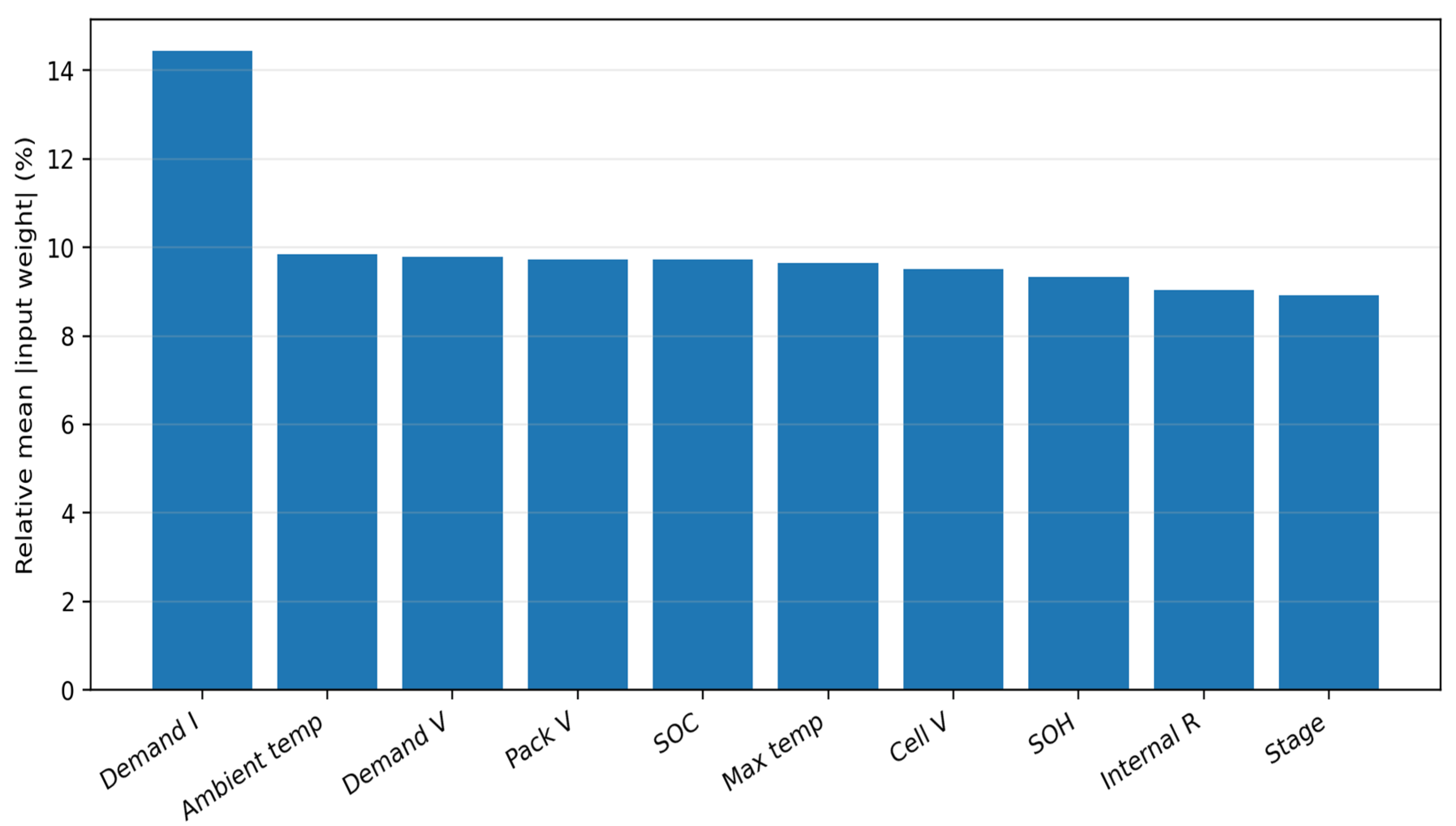
Figure 13 presents the mean absolute first-layer weight magnitude across the 30 HPWOA runs. The demanded current is the largest weight-magnitude input (14.4% of the total), while the remaining inputs each contribute approximately 8.9–9.8%. This weight-based quantity is a model-internal descriptive statistic and does not establish causal importance or prove additional predictive value beyond the requested setpoints.

The repeated weight-magnitude summary should not be interpreted as physical importance: ambient temperature has the second-largest mean magnitude in this model, but the weights are affected by scaling, correlation, and optimizer variability. The result is included only as a transparent description of the fitted HPWOA networks.

4.9. Discussion of Model Behavior and Practical Implications

In the 30-seed FFE-matched sample-level study, the HPWOA has lower error than the WOA and SFSA but higher mean error than standalone PSO. The Adam DO-FNN has the lowest mean test error. These outcomes position the HPWOA as a comparative two-phase baseline, not a novel general-purpose optimizer or an advantage over Adam. The stage-wise findings are stated consistently: Handshake has the highest MAE for both outputs, Recharge has the lowest mean power MAE, and Parameter Configuration has the lowest mean current MAE.

4.10. Physical Consistency and Analytical-Baseline Comparison

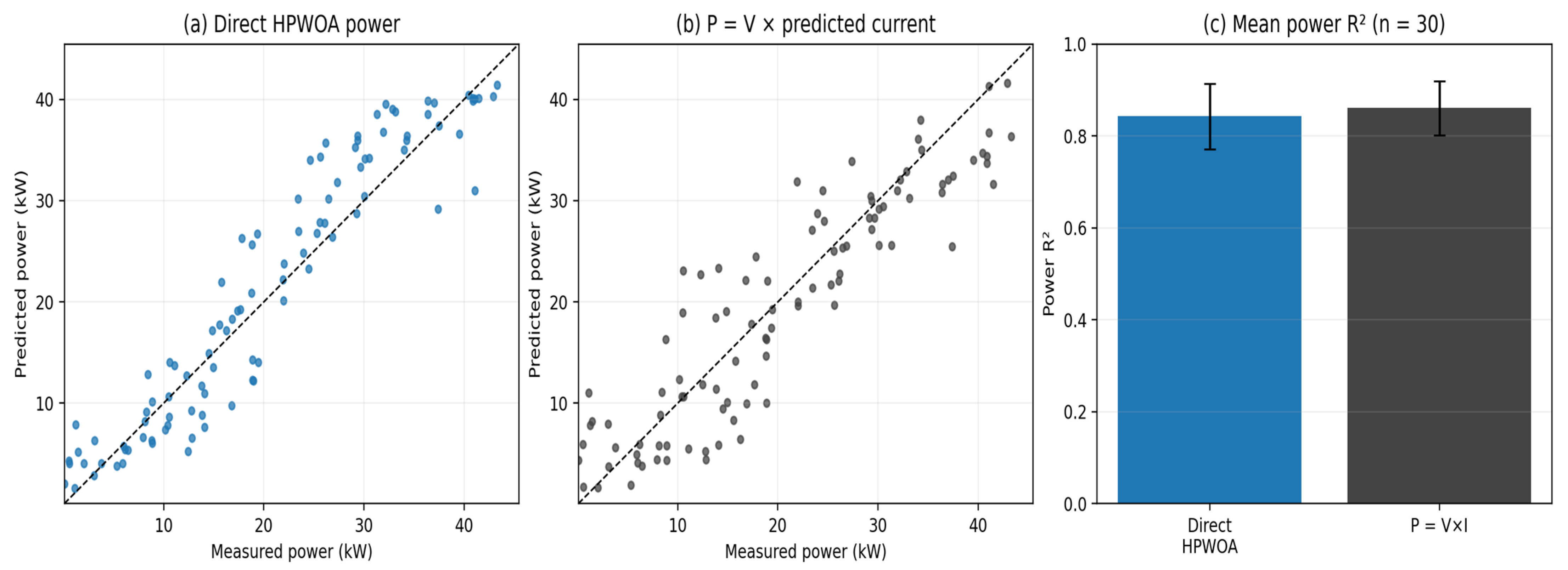
To examine the physical coupling between the delivered power and current (P = V × I), direct HPWOA outputs were compared with an analytical reconstruction using measured pack voltage and HPWOA-predicted current. Across the 30 HPWOA runs, direct power gives R² = 0.843 ± 0.071 and RMSE = 4.658 ± 0.986 kW; the current-derived reconstruction gives R² = 0.861 ± 0.059 and RMSE = 4.385 ± 0.934 kW. The paired power-RMSE difference is not statistically significant (two-sided Wilcoxon p = 0.299). The analytical approach is physically consistent by construction, whereas the direct outputs have a 29.4 ± 14.5% mean discrepancy from V × predicted current. The direct model is, therefore, not presented as a replacement for a physical reconstruction when measured pack voltage is available; disagreement can only be treated as a diagnostic residual.

Table 8. Direct HPWOA and current-derived physical-reconstruction comparison (mean ± SD across 30 HPWOA runs).

Approach	Power R2 (Mean ± SD)	Power RMSE (kW) (Mean ± SD)	Current R2 (Mean ± SD)	Current RMSE (A) (Mean ± SD)	Physical-Consistency Error
Direct HPWOA	0.843 ± 0.071	4.658 ± 0.986	0.858 ± 0.059	12.686 ± 2.687	29.4 ± 14.5%
P = measured V × HPWOA predicted I	0.861 ± 0.059	4.385 ± 0.934	0.858 ± 0.059	12.686 ± 2.687	0% (by construction)

compares the direct HPWOA outputs with the current-derived physical reconstruction to assess predictive accuracy and physical consistency between charging power and current.

Figure 14 compares direct HPWOA power prediction with current-derived power estimation, against measured charging power across 30 independent runs.

4.11. Repeated-Seed and Gradient-Based Benchmark Design

The repeated benchmark uses the fixed 400/100 sample-level split described in Section 3.1 and the 30 independent seeds (1–30). PSO, the WOA, and the HPWOA each use 25 initial candidates plus 150 populations of 25 candidates (3775 FFEs). The SFSA uses 25 initial candidates plus 30 iterations, each with five diffusion candidates per member (also 3775 FFEs). A 10-12-2 ReLU/sigmoid DO-FNN with Xavier-uniform initialization is trained using mini-batch Adam (batch size 32, learning rate 0.003, 600 epochs) on the same normalized training split. The model is evaluated in original physical units after inverse normalization.

Table 9. Five-fold charger-grouped validation (the mean ± standard deviation across the 25 fitted models: five charger folds × five seeds) for the HPWOA and Adam DO-FNN.

Model	Power R2 (Mean ± SD)	Current R2 (Mean ± SD)	Evaluation
HPWOA	0.857 ± 0.045	0.873 ± 0.048	5 charger folds × 5 seeds
Adam DO-FNN	0.983 ± 0.003	0.984 ± 0.001	5 charger folds × 5 seeds

summarizes the five-fold charger-group validation performance of the HPWOA and Adam DO-FNN models across repeated seeds for charging-power and charging-current prediction.

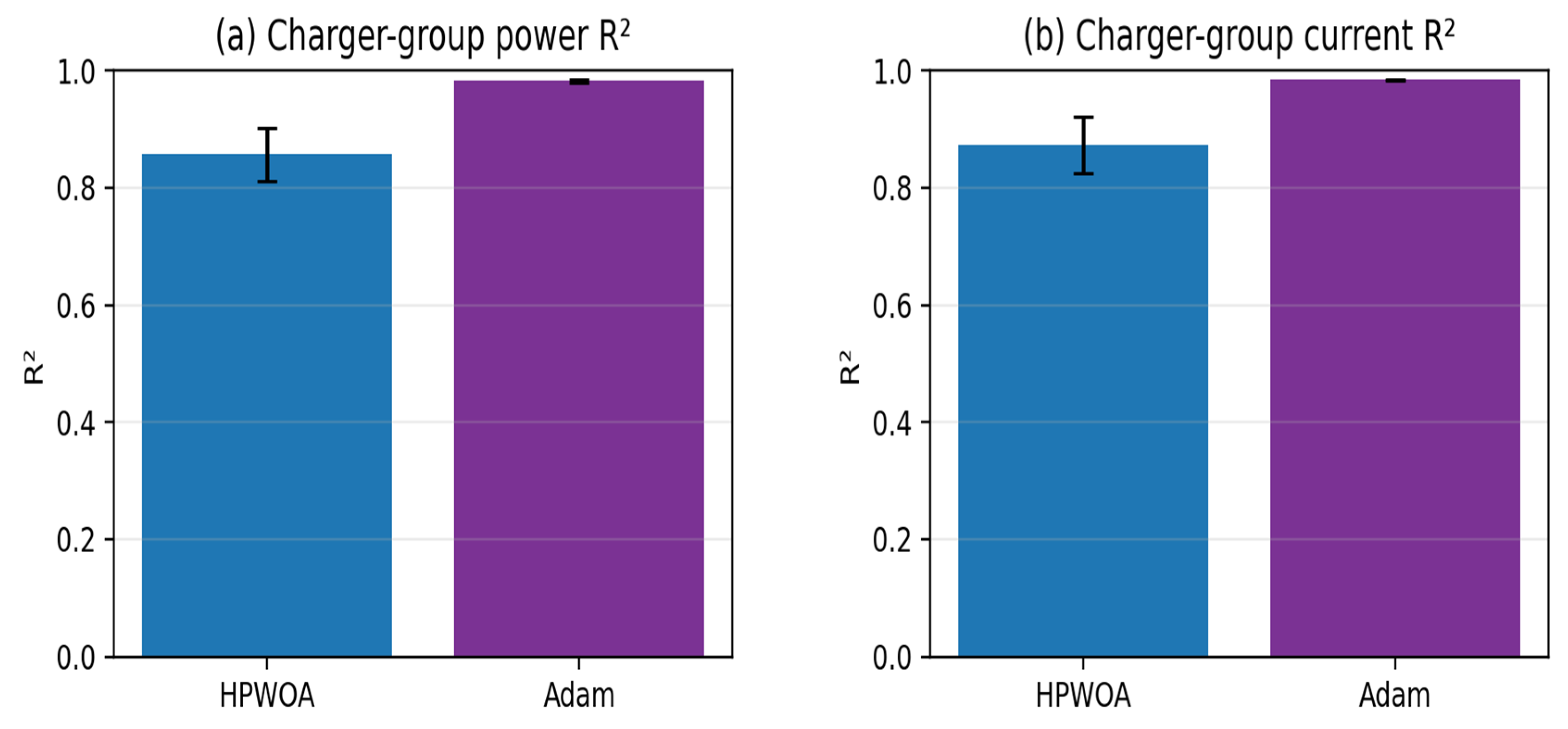
Figure 15 compares the five-fold charger-group predictive performance of HPWOA and Adam for charging power and charging current using R².

4.12. Charger-Grouped Validation

The charger-grouped evaluation uses five GroupKFold partitions formed from ChargerID, with five seeds per fold. The HPWOA obtained the power R² = 0.857 ± 0.045 and the current R² = 0.873 ± 0.048, with RMSE = 4.398 ± 0.719 kW and 11.792 ± 2.062 A. Adam obtained the power R² = 0.983 ± 0.003 and the current R² = 0.984 ± 0.001, with RMSE = 1.551 ± 0.125 kW and 4.221 ± 0.244 A. These results test generalization to unseen chargers, but not to unseen charging sessions or battery cells because the release has no session delimiter and cell identifiers are not grouped in this analysis.

4.13. Limitations of the Results

The revised analysis is reproducible from the supplied public dataset and reports the 30 seeds, FFE-matched metaheuristics, an Adam benchmark, measured runtime, and charger-grouped validation. However, the 500 records remain limited, the timestamps do not identify charging-session boundaries, and the results are generated from one public dataset with a compact 10-12-2 network. The present evidence does not establish session-disjoint, cell-disjoint, cross-dataset, or deployment performance. Future work should use independently collected sessions, group both chargers and cells where appropriate, report more architectures and physical constraints, and evaluate temporal/control performance using session-resolved records.

5. Conclusions and Future Work

This study evaluates a compact dual-output feedforward neural network trained with a fixed 75-iteration PSO phase, followed by a 75-iteration WOA phase. In a reproducible 30-seed FFE-matched sample-level study, the HPWOA outperformed the WOA and SFSA but not standalone PSO. The mini-batch Adam DO-FNN produced the lowest mean test errors: RMSE = 1.704 ± 0.121 kW and 4.946 ± 0.273 A, with R² = 0.980 ± 0.003 and 0.979 ± 0.002, for power and current, respectively. This study, therefore, does not claim a general HPWOA advantage over gradient-based training. The revised stage analysis shows no universal ranking: Handshake has the highest mean MAE for both outputs, Recharge has the lowest mean power MAE, and Parameter Configuration has the lowest mean current MAE. The current-derived P = V × I reconstruction has a slightly lower mean power RMSE than the direct HPWOA output, but the paired difference is not statistically significant (p = 0.299). The direct dual-output configuration should, therefore, be viewed as a comparative soft-sensing and diagnostic model, not a substitute for a physical reconstruction when measured pack voltage is available. The engineering implication is limited but useful: the protocol state and battery-condition variables can be evaluated jointly with requested setpoints in a compact dual-output estimator, while repeated benchmarking prevents a selected stochastic run from being interpreted as general superiority. The repeated evidence supports PSO and especially Adam over the tested HPWOA schedule for this dataset. It does not establish temporal prediction, session-level deployment, or an advantage over a physically constrained reconstruction.

Future work should combine larger independently collected charging-session datasets with charger-, cell-, and session-disjoint validation; constrained multi-output models that enforce P = V × I, where suitable; broad architecture and hyperparameter searches; and time-ordered control-oriented testing. These steps are necessary before direct estimates are integrated into predictive charging supervision or thermal-management scheduling.

References

1. Bhupathi, H.P.; Chinta, S. Smart Charging Revolution: AI and ML Strategies for Efficient EV Battery Use. ESP J. Eng. Technol. Adv. 2022, 2, 154–167. [Google Scholar] [CrossRef]
2. Rajakumari, R.F.; Nithin, K.; Jaganathan, S.; Shagul; Raja, M.A.; Devi, M.R. Performance Analysis of Modern EV Batteries: Efficiency, Longevity, and Future Innovations. Int. J. Syst. Assur. Eng. Manag. 2026, 17, 649–661. [Google Scholar] [CrossRef] [Scilit]
3. Diao, Y. Feasibility Analysis of Various Methods to Extend the Battery Longevity of Electric Vehicles. In Proceedings of the 2nd International Conference on Mechanical, Electronics, and Electrical and Automation Control (METMS 2022), Guilin, China, 7–9 January 2022; SPIE: Bellingham, WA, USA, 2022; Volume 12244, Article 122442U, pp. 686–691. [Google Scholar] [CrossRef] [Scilit]
4. Franzese, P.; Patel, D.D.; Mohamed, A.A.S.; Iannuzzi, D.; Fahimi, B.; Risso, M.; Miller, J.M. Fast DC Charging Infrastructures for Electric Vehicles: Overview of Technologies, Standards, and Challenges. IEEE Trans. Transp. Electrif. 2023, 9, 3780–3800. [Google Scholar] [CrossRef] [Scilit]
5. Rachid, A.; El Fadil, H.; Gaouzi, K.; Rachid, K.; Lassioui, A.; El Idrissi, Z.; Koundi, M. Electric Vehicle Charging Systems: Comprehensive Review. Energies 2023, 16, 255. [Google Scholar] [CrossRef] [Scilit]
6. Mdallal, A.; Yasin, A.; Alaboudy, A.H.K.; ElSaid, K. Advancements in EV Charging Standards and Technologies for Sustainable Transportation. Renew. Sustain. Energy Technol. 2026, 2, 2. [Google Scholar] [CrossRef] [Scilit]
7. Mohan, A.; Pal, K.; Meena, H.K. Comprehensive Review of Electric Vehicle Charging Infrastructure: Technologies, Standards, and Smart Energy Management. Future Batter. 2026, 10, 100177. [Google Scholar] [CrossRef] [Scilit]
8. Waseem, M.; Sreeshobha, E.; Shashidhar Reddy, K.; Donateo, T. State-of-the-Art and Advancement of Charging Infrastructure in Electric Mobility: An Integrated Review. Energies 2024, 17, 6137. [Google Scholar] [CrossRef] [Scilit]
9. Ok, S.; Vennilashree, S. A Review on Electric Vehicles: Technologies and Challenges. Lex Localis-J. Local Self-Gov. 2025, 23, 2060–2094. [Google Scholar] [CrossRef] [Scilit]
10. Mamin, I. Dynamic Load Management System for EV Chargers. Bachelor’s Thesis, Laurea University of Applied Sciences, Vantaa, Finland, 2026; 66p. URN:NBN:fi:amk-202602132831. [Google Scholar]
11. Dini, P.; Saponara, S.; Colicelli, A. Overview on Battery Charging Systems for Electric Vehicles. Electronics 2023, 12, 4295. [Google Scholar] [CrossRef] [Scilit]
12. Almaktoof, A.; Taha, M.; Adonis, M.; Halablab, K. A Hybrid EV Charging Architecture Integrating DC Fast Charging and Wireless Power Transfer. Energy Sci. Eng. 2026, 14, 3013–3027. [Google Scholar] [CrossRef] [Scilit]
13. Nasr Esfahani, F. High Power Density On-Board Chargers (OBCs) for Electric Vehicles (EVs). Ph.D. Thesis, Lancaster University, Lancaster, UK, 2025. [Google Scholar] [CrossRef]
14. Yilmaz, M.; Krein, P.T. Review of Battery Charger Topologies, Charging Power Levels, and Infrastructure for Plug-In Electric and Hybrid Vehicles. IEEE Trans. Power Electron. 2013, 28, 2151–2169. [Google Scholar] [CrossRef] [Scilit]
15. Hu, X.; Johannesson, L.; Murgovski, N.; Egardt, B. Longevity-Conscious Dimensioning and Power Management of the Hybrid Energy Storage System in a Fuel Cell Hybrid Electric Bus. Appl. Energy 2015, 137, 913–924. [Google Scholar] [CrossRef] [Scilit]
16. Calborean, A.; Máthé, L.; Bruj, O. Phase Change Materials for Thermal Management in Lithium-Ion Battery Packs: A Review. Batteries 2025, 11, 432. [Google Scholar] [CrossRef] [Scilit]
17. Patra, B.B.; Vaidya, V.; Hussain, M.; Gori, Y. Battery Thermal Management in Hybrid Electric Vehicles. In Thermal Battery Management System for Hybrid and Electric Vehicles; Kumar, A., Awasthi, M.K., Dutt, N., Singla, Y.K., Thangavel, S., Eds.; John Wiley & Sons: Hoboken, NJ, USA, 2025; pp. 133–156. [Google Scholar] [CrossRef] [Scilit]
18. Senol, M.; Bayram, I.S.; Naderi, Y.; Galloway, S. Electric Vehicles under Low Temperatures: A Review on Battery Performance, Charging Needs, and Power Grid Impacts. IEEE Access 2023, 11, 39879–39912. [Google Scholar] [CrossRef] [Scilit]
19. Zou, C.; Manzie, C.; Nešić, D.; Kallapur, A.G. Multi-Time-Scale Observer Design for State-of-Charge and State-of-Health of a Lithium-Ion Battery. J. Power Sources 2016, 335, 121–130. [Google Scholar] [CrossRef] [Scilit]
20. Kumar, R.R.; Ravi Kumar, R.K.; Bharatiraja, C.; Udhayakumar, K.; Devakirubakaran, S.; Sekar, K.S.; Mihet-Popa, L. Advances in Batteries, Battery Modeling, Battery Management System, Battery Thermal Management, SOC, SOH, and Charge/Discharge Characteristics in EV Applications. IEEE Access 2023, 11, 105761–105809. [Google Scholar] [CrossRef] [Scilit]
21. Adaikkappan, M.; Sathiyamoorthy, N. Modeling, State of Charge Estimation, and Charging of Lithium-Ion Battery in Electric Vehicle: A Review. Int. J. Energy Res. 2022, 46, 2141–2165. [Google Scholar] [CrossRef] [Scilit]
22. IEC 61851-1:2017; Electric Vehicle Conductive Charging System-Part 1: General Requirements. International Electrotechnical Commission: Geneva, Switzerland, 2017.
23. Wang, H.; Guo, B.; Zhou, X.; Wang, S.; Hong, Z.; He, T. Resource-Oriented Optimization of Electric Vehicle Systems: A Data-Driven Survey on Charging Infrastructure, Scheduling, and Fleet Management. arXiv 2025, arXiv:2509.04533. [Google Scholar] [CrossRef] [Scilit]
24. Shan, C.; Chin, C.S.; Mohan, V.; Zhang, C. Review of Various Machine Learning Approaches for Predicting Parameters of Lithium-Ion Batteries in Electric Vehicles. Batteries 2024, 10, 181. [Google Scholar] [CrossRef] [Scilit]
25. Shen, P.; Ouyang, M.; Lu, L.; Li, J.; Feng, X. The Co-Estimation of State of Charge, State of Health, and State of Function for Lithium-Ion Batteries in Electric Vehicles. IEEE Trans. Veh. Technol. 2018, 67, 92–103. [Google Scholar] [CrossRef] [Scilit]
26. Goodfellow, I.; Bengio, Y.; Courville, A. Deep Learning; MIT Press: Cambridge, MA, USA, 2016. [Google Scholar]
27. Bilal, M.; Bokoro, P.N.; Sharma, G. Hybrid Optimization for Sustainable Design and Sizing of Standalone Microgrids Integrating Renewable Energy, Diesel Generators, and Battery Storage with Environmental Considerations. Results Eng. 2025, 25, 103764. [Google Scholar] [CrossRef] [Scilit]
28. Zara2099. EV Battery Charging & Thermal Runaway Dataset. Kaggle. 2025. Available online: https://www.kaggle.com/datasets/zara2099/ev-battery-charging-and-thermal-runaway-dataset (accessed on 13 July 2026).
29. Tian, M.; Zhang, Q.; Tian, D.; Jin, L.; Li, J.; Xiao, F. Pre-Stability Control for In-Wheel-Motor-Driven Electric Vehicles with Dynamic State Prediction. IEEE Trans. Intell. Veh. 2024, 9, 4541–4554. [Google Scholar] [CrossRef] [Scilit]
30. Zhang, Q.; Yao, Y.; Wang, J.; Pi, D.; Yin, G. Adaptive Hybrid Model-Based and Data-Driven Clamping Force Estimation for Electromechanical Brake Systems. IEEE Trans. Ind. Electron. 2026, 1–12. [Google Scholar] [CrossRef] [Scilit]
Figure 1. Dataset overview: (a) number of samples by charging stage; (b) demanded and delivered charging current by stage; and (c) state of charge versus delivered charging power.
Wevj 17 00440 g001
Figure 2. Stage-wise distributions: (a) delivered charging power; (b) delivered charging current; and (c) maximum battery temperature.
Wevj 17 00440 g002
Figure 3. HPWOA-optimized dual-output feedforward neural network architecture.
Wevj 17 00440 g003
Figure 4. A schematic overview of PSO, WOA, SFSA, and the proposed HPWOA optimization strategy.
Wevj 17 00440 g004
Figure 5. Dual-output problem formulation and evaluation pipeline.
Wevj 17 00440 g005
Figure 6. Repeated FFE-matched convergence comparison (n = 30): (a) mean best training MSE against fitness-function evaluations, with ±1 SD bands; (b) final training MSE (mean ± SD); and (c) measured computation time per run (mean ± SD). PSO, WOA, and HPWOA use 150 iterations; SFSA uses 30 iterations with five diffusion candidates per individual, giving all metaheuristics 3775 FFEs.
Wevj 17 00440 g006
Figure 7. The representative predicted versus measured charging power on the 100-sample test set: (a) PSO; (b) the WOA; (c) the SFSA; (d) the HPWOA; and (e) the mini-batch Adam DO-FNN. The representative seeds are selected by the median normalized test MSE; the reference line denotes perfect agreement.
Wevj 17 00440 g007
Figure 8. The representative predicted versus measured charging current on the 100-sample test set: (a) PSO; (b) the WOA; (c) the SFSA; (d) the HPWOA; and (e) the mini-batch Adam DO-FNN. The representative seeds are selected by the median normalized test MSE; the reference line denotes perfect agreement.
Wevj 17 00440 g008
Figure 9. HPWOA residual plots for the two predicted outputs: (a) C h a r g e P o w e r k W , and (b) C h a r g e C u r r e n t A . The residuals are computed as the measured value minus the predicted value.
Wevj 17 00440 g009
Figure 10. The thirty-seed regression-metric comparison (mean ± SD): (a) the charging-power RMSE; (b) the charging-power MAE; (c) the charging-power R2; (d) the charging-current RMSE; (e) the charging-current MAE; and (f) the charging-current R2. The results include PSO, the WOA, the SFSA, the HPWOA, and the mini-batch Adam DO-FNN.
Wevj 17 00440 g010
Figure 11. The ordered test-sample comparison of the two EV fast-charging targets across the 100-sample test set: (a) the charging power, and (b) the charging current. The representative runs are shown for PSO, the WOA, the SFSA, the HPWOA, and Adam; the horizontal axis is a display index, not time.
Wevj 17 00440 g011
Figure 12. The HPWOA per-stage MAEs for the two predicted targets: (a) C h a r g e P o w e r k W , and (b) C h a r g e C u r r e n t A . The four protocol stages are Handshake, Parameter Configuration, Recharge, and End of Charge.
Wevj 17 00440 g012
Figure 13. Mean relative absolute first-layer weight magnitude across 30 HPWOA runs. Values are descriptive network weights, not causal feature-importance estimates.
Wevj 17 00440 g013
Figure 14. Direct HPWOA and current-derived physical-reconstruction comparison: (a) representative direct HPWOA power versus measured power; (b) representative P = V × predicted-current power versus measured power; and (c) mean power R2 (±1 SD) across 30 HPWOA runs.
Wevj 17 00440 g014
Figure 15. Five-fold charger-grouped R2 (the mean ± standard deviation across five seeds per fold) for the HPWOA and Adam DO-FNN: (a) charging power, and (b) charging current.
Wevj 17 00440 g015