Unified Experimentally Constrained PID/LQR Optimization for MRD-Based Semi-Active Suspension Control in Electric Vehicles

Abstract

The rapid adoption of electric vehicles, together with increased battery mass and altered load distribution, is placing greater demands on ride comfort and suspension adaptability, while controller optimization may still request forces beyond the instantaneous capability of the physical semi-active actuator if experimentally supported force limits are not explicitly enforced. This study proposes a unified experimentally constrained optimization framework for a magnetorheological damper (MRD)-based semi-active suspension system using a two-degree-of-freedom quarter-car model. The damper is characterized at eleven current levels and represented by a branch-dependent lookup model that provides the zero-current baseline and instantaneous feasible force range. Proportional–integral–derivative (PID) and linear quadratic regulator (LQR) controllers are independently tuned using a genetic algorithm (GA) and particle swarm optimization (PSO) under identical vehicle dynamics, objective functions, tuning excitation, and MRD force constraints. Each candidate force demand is projected onto the experimentally derived feasible range throughout optimization. The controllers are tuned on a composite B–C–D profile and subsequently evaluated over nine road–speed scenarios. PID-PSO reduces the RMS sprung-mass acceleration by 15.91% and achieves the best acceleration performance in six cases, whereas LQR-PSO provides more balanced improvements in body motion, suspension travel, tire response, and force feasibility. The proposed framework therefore provides a more physically constrained basis for the comparative design and evaluation of MRD-based semi-active suspension control.

1. Introduction

The transition toward electrified and increasingly automated road vehicles is increasing the demand for ride comfort, chassis adaptability, and stable tire–road interaction over a wide range of operating conditions [1,2,3,4,5]. In electric vehicles, battery mass and modified load distribution can amplify the importance of vertical vibration control, while integrated and preview-based chassis functions require the suspension to respond effectively to changing road excitation rather than rely on a single fixed mechanical calibration.

Vehicle suspension design inherently involves a compromise between vibration isolation and road holding. Passive systems provide only a fixed balance between these competing requirements [6,7], whereas semi-active suspensions can adjust their dissipative characteristics in real time with substantially lower energy demand than fully active systems. Recent studies have shown the effectiveness of preview information and advanced control strategies under varying road excitation [8]. Among semi-active actuators, magnetorheological dampers (MRDs) are particularly attractive because their force characteristics can be rapidly adjusted through the applied magnetic field and integrated into real-time control frameworks [9]. Since suspension performance also influences wheel-load variation and tire–road interaction, body-vibration reduction should be assessed together with suspension travel and tire response [10]. Consequently, MRD-based semi-active suspension remains an important research direction in adaptive vehicle chassis systems [11].

Research on MRD-based suspension systems has focused strongly on accurately representing their nonlinear, current-dependent, and hysteretic force behavior. Frequency-dependent Bouc–Wen models [12], non-parametric data-driven approaches [13], experimental vibration-control studies [14], and hardware developments aimed at improving force range and structural performance [15,16,17,18] have all contributed to this direction. Higher-fidelity analytical formulations [19] and inverse MRD models integrated with optimized controllers [20] have also been reported. These studies highlight the importance of both damper design and force representation; however, for repeated controller evaluation, experimentally derived data-driven models provide a direct means of preserving measured branch dependence without repeatedly identifying analytical hysteresis parameters.

At the control level, a wide range of strategies has been investigated, including MRD signal-path design [21], fuzzy neural network PID control [22], variable-universe fuzzy PID control [23], optimization-based PID tuning [24], skyhook control [25], preview-based predictive control [26], comparative controller optimization [27], and optimization-assisted LQR design [28]. These studies show that PID- and LQR-based structures remain valuable control benchmarks, but their performance depends strongly on parameter tuning, objective formulation, operating conditions, and actuator representation. This sensitivity has motivated extensive use of derivative-free metaheuristic methods. Genetic algorithms have been applied to nonlinear suspension optimization and processor-in-the-loop evaluation [29,30], while particle swarm optimization (PSO) has been used for MRD suspension optimization [31], damper parameter identification [32], and comparative PID tuning [33]. Road roughness and vehicle speed must also be considered because excitation severity can alter both absolute response levels and the relative effectiveness of competing controllers [34].

Despite this progress, existing studies employ different combinations of controller structure, optimizer, actuator model, objective function, excitation condition, and constraint-handling procedure, which makes direct comparison difficult [21,22,23,24,25,26,27,28,29,30,31,32,33]. Moreover, the use of an MRD lookup model does not by itself ensure that controller optimization respects the instantaneous experimentally supported force capability of the physical damper, because controller force demand is not always evaluated against this state-dependent limit during optimization. In the present framework, the experimentally measured branch-dependent characteristics are instead used to determine the zero-current baseline $F_{0A}$ and the instantaneous attainable forces $F_{min}$ and $F_{max}$ from the current relative displacement and velocity. The desired controller correction force is then projected onto this experimentally supported interval at every simulation step and during every candidate evaluation. Consequently, the optimization is performed on the realized semi-active response and its force compatibility rather than on an unrestricted force command or a generic fixed actuator bound.

Accordingly, the present study focuses on a controlled evaluation rather than a comprehensive ranking of semi-active control strategies. PID and LQR are selected as two representative controller structures and independently tuned by GA and PSO. The four controller–optimizer configurations are compared under the same vehicle model, objective function, tuning excitation, optimization budget, and experimentally derived MRD force-realization framework, and are subsequently evaluated across varying road and speed scenarios.

The main contributions of this work are: (i) an experimental characterization and branch-dependent force representation of a custom-built MR damper over the full tested current range; (ii) a unified optimization framework in which the experimentally derived MRD force limits are incorporated consistently into the evaluation of PID- and LQR-based candidates tuned by GA and PSO; and (iii) a consistent comparison of tuning performance, dynamic response, force feasibility, and cross-condition robustness. The proposed framework therefore evaluates vibration attenuation and MRD force attainability within the same optimization and validation process.

2. Vehicle Vibration Model

To isolate the dominant vertical dynamics at a single wheel station while maintaining a compact and computationally efficient framework for repeated force-constrained optimization, a two-degree-of-freedom quarter-car model is adopted. This model captures the primary interaction between the sprung and unsprung masses, suspension compliance, and tire stiffness, while excluding pitch, roll, and inter-axle coupling effects. The quarter-car formulation is also relevant to practical semi-active suspension systems, in which each suspension corner can be equipped with an independently controlled actuator that adapts its damping force to the local wheel and body responses. This suspension-corner representation is deliberately retained for the present controlled comparison because it captures the dominant local vertical dynamics governing MRD force realization while allowing repeated PID/LQR optimization by GA and PSO under identical conditions. A full-vehicle formulation would additionally introduce pitch and roll motions, load transfer, inter-axle coupling, and control-allocation effects, thereby broadening the analysis beyond the suspension-corner-level interaction targeted in the present framework. The adopted parameter set represents a control-oriented compact battery-electric passenger vehicle rather than a specific production model. Under a symmetric four-corner assumption, the parameters correspond to an equivalent total modeled vehicle mass of 1396 kg.

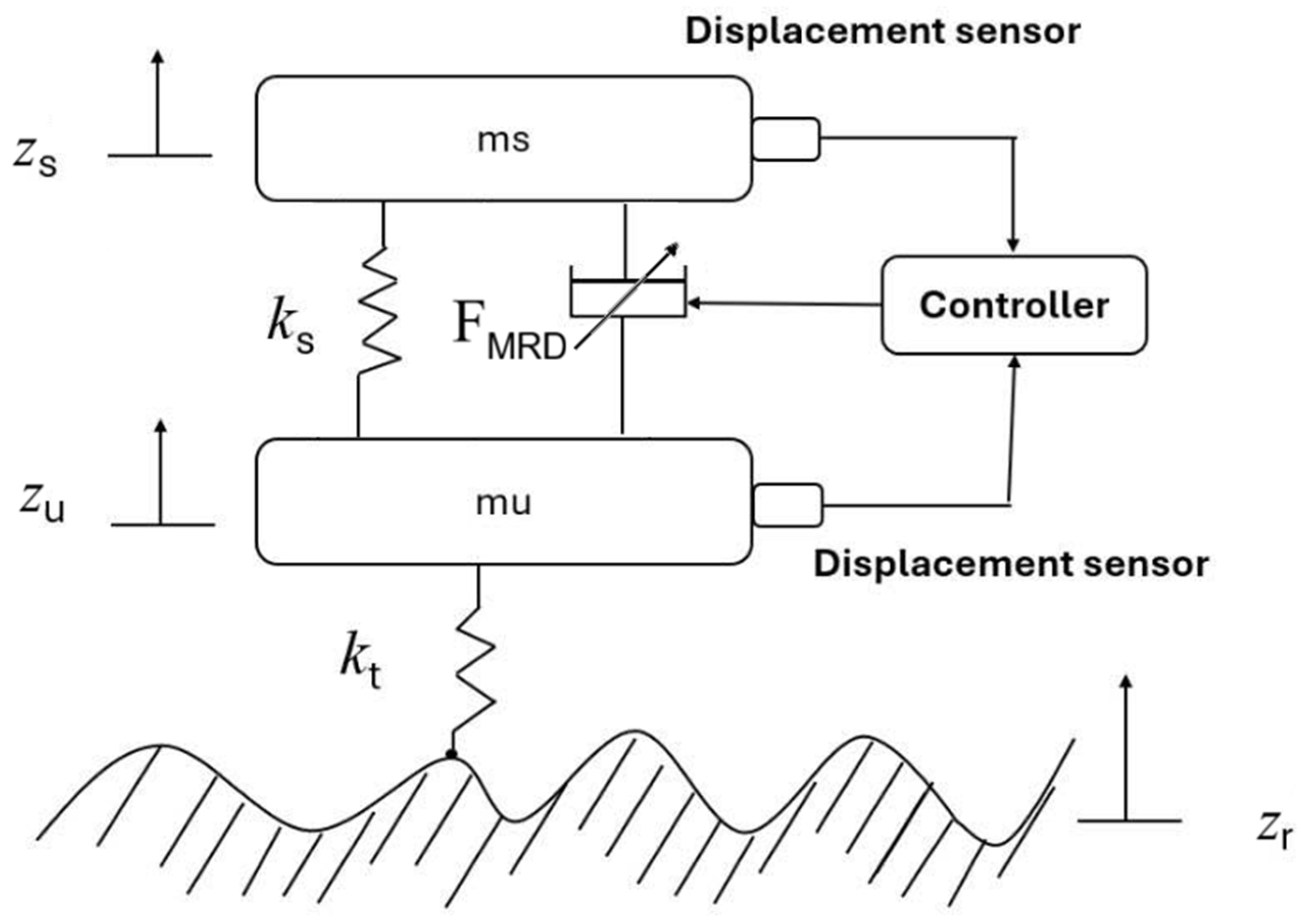
The model consists of the sprung mass $m_s$, representing the vehicle-body mass supported by one wheel station, and the unsprung mass $m_u$, representing the wheel, hub, and associated components. Their vertical displacements are denoted by $z_s$ and $z_u$, respectively, while $z_r$ represents the road displacement input. The suspension spring and tire are modeled as linear elastic elements with stiffnesses $k_s$ and $k_t$, respectively. Tire damping is neglected, consistent with the control-oriented focus on the dominant vertical suspension dynamics. The schematic representation and sign convention are shown in Figure 1.

The MR damper is installed between the sprung and unsprung masses, with its mechanical operating state described by the relative displacement $z_s-z_u$ and relative velocity ${\dot{z}}_s-{\dot{z}}_u$. The suspension travel and tire deflection are represented by $z_s-z_u$ and $z_u-z_r$, respectively. Unlike a conventional quarter-car model with a fixed viscous damping coefficient, the present formulation directly incorporates the nonlinear MRD force $F_{MRD}$. A positive $F_{MRD}$ is defined as acting downward on the sprung mass and upward on the unsprung mass. Accordingly, the equations of motion are

$$\left\{\begin{array}{c}{m}_s{\ddot{z}}_s=-k_s(z_s-z_u)-F_{MRD}\\ m_u{\ddot{z}}_u=k_s(z_s-z_u)+F_{MRD}-k_t(z_u-z_r)\end{array}\right.$$

(1)

The force in Equation (1) is obtained from the experimentally characterized MRD data, with the measured zero-current response $F_{0A}$ used as the baseline condition. In this study, the passive reference therefore denotes the physical MRD operated continuously at 0 A, which retains its measured non-zero damping behavior, rather than an idealized linear viscous damper. The experimental force representation is described in Section 3, while the controller-based force realization is presented in Section 4.3. For the LQR formulation and time-domain simulation, the state vector is defined as

$$x={\left[\begin{array}{cccc}{z}_s& {\dot{z}}_s& z_u& {\dot{z}}_u\end{array}\right]}^T$$

(2)

The system of Equation (1) can then be expressed in state-space form as

$$\dot{x}=Ax+B{F}_{MRD}+E{z}_r$$

(3)

where $A$ is the system matrix, $B$ is the MRD force input matrix, and $E$ is the road input matrix, defined as follows:

$$A=\left[\begin{array}{cccc}0& 1& 0& 0\\ -{\displaystyle \frac{k_s}{m_s}}& 0& {\displaystyle \frac{k_s}{m_s}}& 0\\ 0& 0& 0& 1\\ {\displaystyle \frac{k_s}{m_u}}& 0& -{\displaystyle \frac{k_s+k_t}{m_u}}& 0\end{array}\right], B=\left[\begin{array}{c}0\\ -{\displaystyle \frac{1}{m_s}}\\ 0\\ {\displaystyle \frac{1}{m_u}}\end{array}\right], E=\left[\begin{array}{c}0\\ 0\\ 0\\ {\displaystyle \frac{k_t}{m_u}}\end{array}\right]$$

(4)

The opposite signs of the non-zero terms in $B$ represent the equal and opposite actions of the MRD force on the sprung and unsprung masses. The road displacement enters the system through the tire stiffness and therefore acts directly on the unsprung-mass dynamics.

The principal response quantities used for controller evaluation are the sprung-mass acceleration ${\ddot{z}}_s$, velocity ${\dot{z}}_s$, and displacement $z_s$, together with the suspension travel $z_s-z_u$ and tire deflection $z_u-z_r$. These responses are used to quantify ride-oriented body motion, suspension working space, and tire behavior. Their RMS and peak evaluation metrics are defined in Section 4.5. The quarter-car parameters used throughout the simulations are summarized in

Table 1. Quarter-car model parameters.

Parameter	Description	Value	Unit
$m_s$	Sprung mass	290	kg
$m_u$	Unsprung mass	59	kg
$k_s$	Suspension spring stiffness	16,812	N/m
$k_t$	Tire stiffness	190,000	N/m

.

3. Experimental Characterization of MRD Damping Characteristics

The MR damper used in this study was a custom-built prototype manufactured specifically for the present experimental program. Its damping force depends on piston displacement, piston velocity, motion branch, and coil current; these relationships determine both the zero-current baseline and the force range available to the semi-active controller.

The prototype was characterized over eleven current levels from 0 to 2 A in 0.2 A increments, with piston-velocity and displacement ranges of −0.3 to 0.3 m/s and −100 to 100 mm, respectively.

Table 2. Main information and characterization ranges of the custom-built MR damper.

Parameter	Value	Unit
Damper type	Custom-built MRD prototype	–
Coil-current range	0–2	A
Current increment	0.2	A
Number of current levels	11	–
Piston-velocity range	−0.3 to 0.3	m/s
Displacement range	−100 to 100	mm
Data points per current level	1000	–

summarizes the main prototype information and tested operating ranges.

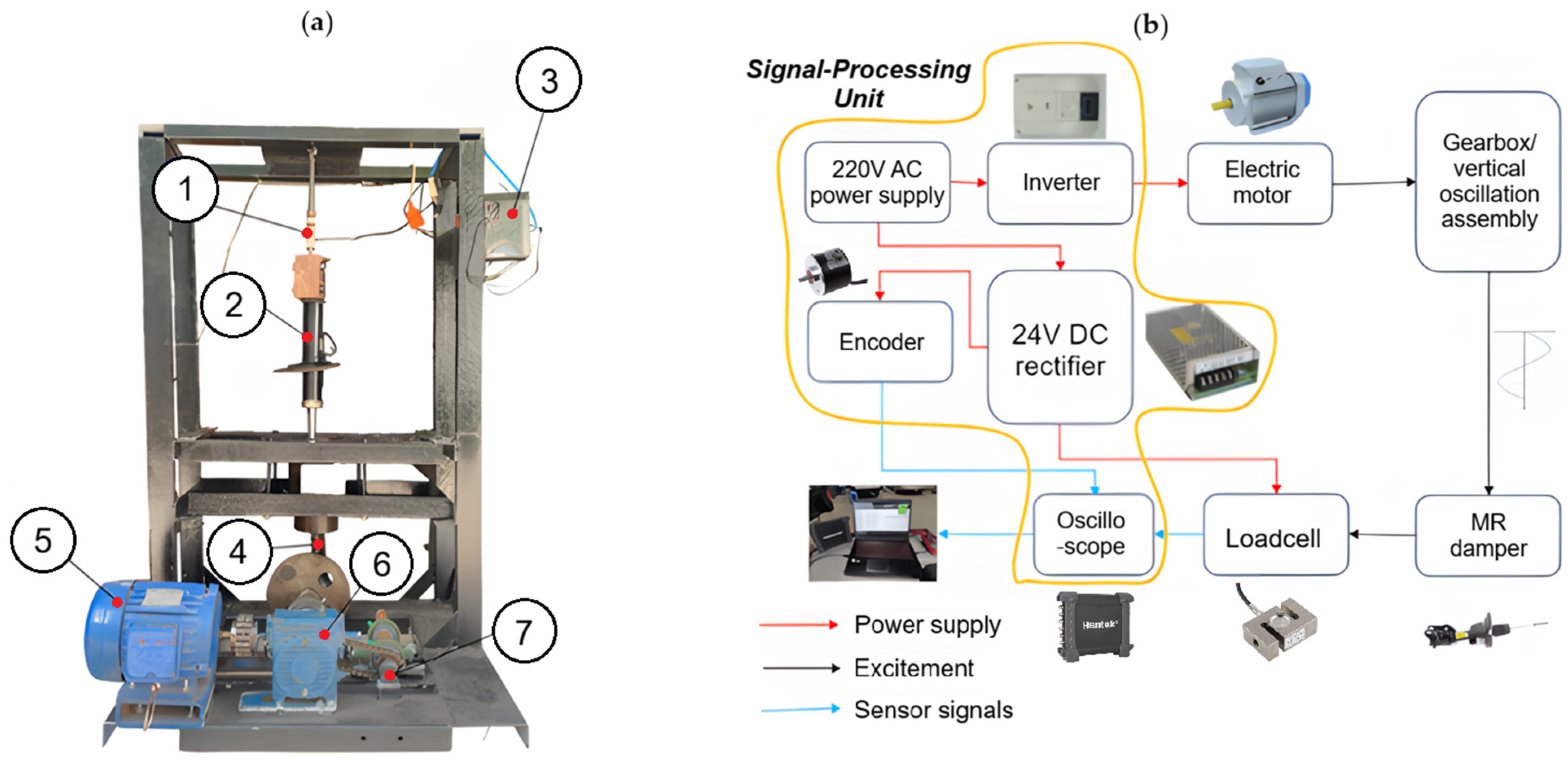
The experiments were conducted on the MR damper test bench at Hanoi University of Science and Technology. The bench is driven by a 1.7 kW electric motor and has a rated test load of 2.5 kN. During operation, the motor drives the gearbox and crank-slider mechanism, which converts rotary motion into controlled reciprocating motion of the damper piston. The resulting damping force and piston motion are measured synchronously, conditioned, and acquired by the data-acquisition system before being transferred to a host computer for real-time monitoring and subsequent processing. The same excitation and measurement chain is maintained throughout the current sweep to ensure consistent comparison of the force characteristics obtained at different current levels. Figure 2a shows the test rig and its principal mechanical and measurement components, while Figure 2b summarizes the power-supply, excitation, and measurement-signal paths used for synchronous acquisition of force and motion data.

During each test, the damper was subjected to periodic reciprocating motion while the coil current was held constant. Eleven current levels from 0 to 2 A were applied in 0.2 A increments, as defined in Equation (5), and force, piston displacement, and piston velocity were recorded synchronously over the same excitation cycle.

$$I_m=0.2m \left(A\right), m=0,1,\dots ,10$$

(5)

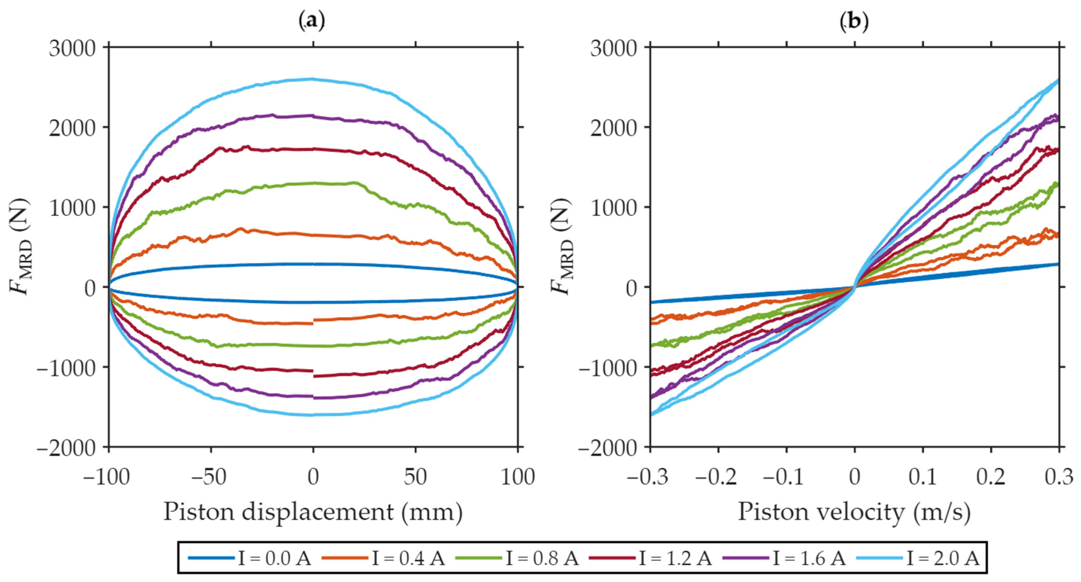
After the initial transient was removed, one representative record containing 1000 operating points was retained for each current level. Figure 3 presents the measured characteristics at six representative currents. The force–displacement loops in Figure 3a broaden as current increases, while the force–velocity curves in Figure 3b show the nonlinear increase in damping force and the distinct compression and rebound branches. The complete eleven-level dataset is retained for the lookup procedure.

The synchronized force, displacement, and velocity records are used directly as the experimental database; no analytical hysteresis equation is identified. Instead, the measured data are classified by operating branch and interpolated at each simulation step.

At simulation step $k$, the active hysteresis branch is selected from the signs of the suspension relative displacement and relative velocity according to Equation (6).

This four-branch classification retains the measured hysteresis dependence on both motion direction and displacement state. At the switching boundaries, the non-overlapping inequalities in Equation (6) assign zero relative velocity to the nonnegative-velocity branches and zero relative displacement to the nonnegative-displacement branches, so that each operating point is uniquely assigned to one branch. No interpolation or blending is performed across branch boundaries.

$$b_k=\left\{\begin{array}{cc}1,& {\dot{z}}_{s,k}-{\dot{z}}_{u,k}<0,z_{s,k}-z_{u,k}<0\\ 2,& {\dot{z}}_{s,k}-{\dot{z}}_{u,k}\ge 0,z_{s,k}-z_{u,k}<0\\ 3,& {\dot{z}}_{s,k}-{\dot{z}}_{u,k}\ge 0,z_{s,k}-z_{u,k}\ge 0\\ 4,& {\dot{z}}_{s,k}-{\dot{z}}_{u,k}<0,z_{s,k}-z_{u,k}\ge 0\end{array}\right.$$

(6)

For the selected branch, the instantaneous relative velocity is first restricted to the measured branch-specific range, as defined in Equation (7), thereby preventing evaluation outside the experimental velocity domain. No interpolation is performed between different hysteresis branches; therefore, the measured branch dependence is retained explicitly.

$${\overline{v}}_k=min\left[max\left({\dot{z}}_{s,k}-{\dot{z}}_{u,k},v_{min}\right),v_{max}\right]$$

(7)

For each tested current level, the corresponding damper force is obtained by linear interpolation between the adjacent measured force–velocity samples of the active branch, as given by Equation (8). The interpolation is therefore local rather than a global linear approximation of the MRD hysteresis. The experimental database provides approximately 249–250 unique velocity samples per branch, with a velocity spacing of approximately $1.20\times {10}^{-3}$ m/s.

$${\widehat{F}}_{k,m}=F_{j,m}^{\left(b_k\right)}+{\displaystyle \frac{{\overline{v}}_k-v_j^{\left(b_k\right)}}{v_{j+1}^{\left(b_k\right)}-v_j^{\left(b_k\right)}}}\left(F_{j+1,m}^{\left(b_k\right)}−F_{j,m}^{\left(b_k\right)}\right)$$

(8)

A leave-one-out reconstruction check was additionally performed to assess the interpolation choice. Linear interpolation yielded an overall MAE of 2.89 N and RMSE of 4.45 N, compared with 2.98 N and 4.58 N for PCHIP and 3.29 N and 5.12 N for cubic-spline interpolation, respectively. Linear interpolation was therefore retained because it provides the lowest reconstruction error for the present dataset while avoiding additional high-order curvature between measured samples. The resulting reconstruction errors are small relative to the measured MRD force range and affect the optimization only through local variations in $F_{0A}$, $F_{min}$, and $F_{max}$. Because the same interpolation procedure is applied to every candidate and all four controller–optimizer configurations, this interpolation uncertainty is common to the comparative evaluation and is expected to have limited influence on the resulting comparative conclusions.

The interpolated force at 0 Ampe defines $F_{0A}$, which represents the measured zero-current MRD baseline and is used both as the passive reference and as the reference force for the controller correction-force formulation, as expressed in Equation (9).

$$F_{0A,k}={\widehat{F}}_{k,0}$$

(9)

The lower and upper attainable forces at the same operating state are obtained from the complete set of interpolated current-dependent forces according to Equation (10).

$$F_{min,k}=\underset{m=0,\dots ,10}{min}\left({\widehat{F}}_{k,m}\right),F_{max,k}=\underset{m=0,\dots ,10}{max}\left({\widehat{F}}_{k,m}\right)$$

(10)

The branch-dependent lookup procedure therefore provides the zero-current baseline force and the lower and upper attainable forces $F_{min}$ and $F_{max}$ at the current damper operating state. Because the relative velocity is restricted to the measured branch-specific range before interpolation, the returned force values remain within the experimentally characterized velocity domain. Figure 3 summarizes the measured force–displacement and force–velocity characteristics used to construct this lookup database.

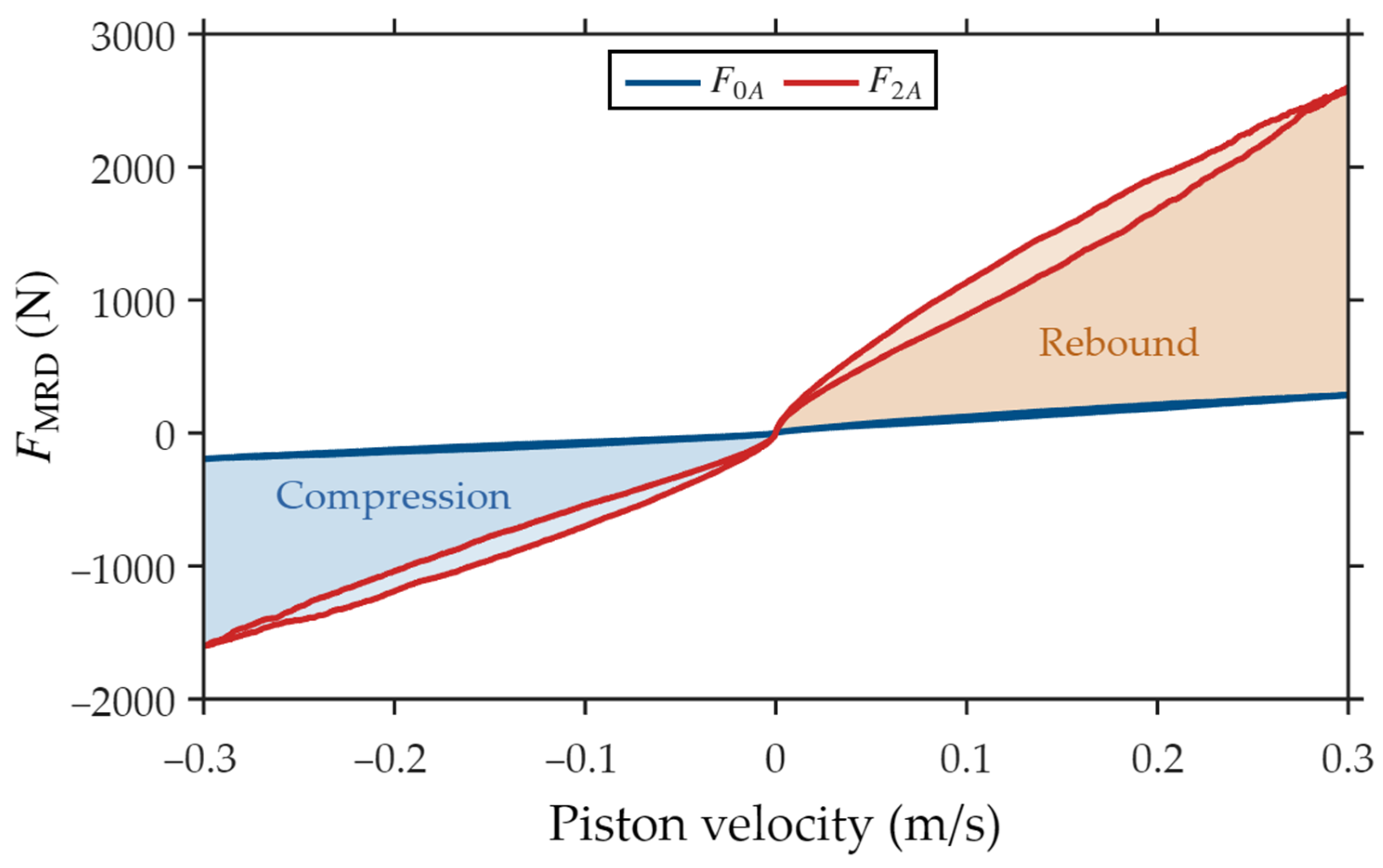
Figure 4 illustrates the experimentally supported force envelope derived from the measured MRD characteristics. The 0 A characteristic provides the baseline force, while the current-dependent characteristics define the attainable force range in compression and rebound. The shaded region represents the available force variation at each operating velocity and hysteresis branch. These experimentally derived quantities form the force database subsequently used by the semi-active control framework in Section 4.

4. Semi-Active Control and Optimization Framework

4.1. PID Controller

The PID controller generates a desired correction force from the sprung-mass motion, following the conventional PID feedback structure widely applied in suspension-control and optimization studies [24,33]. The feedback variable is the sprung-mass velocity, and its desired value is set to zero so that the control objective is to suppress vertical body motion. The control error is defined in Equation (11).

$$e\left(t\right)={\dot{z}}_s\left(t\right)-{\dot{z}}_{s,ref}\left(t\right)={\dot{z}}_s\left(t\right)$$

(11)

Because the reference sprung-mass velocity is zero, the error is equal to the instantaneous sprung-mass velocity. The continuous-time PID correction-force law is written as

$$\mathsf{\Delta }{F}_{PID}(t)=K_{p}e(t)+K_i{\int }_0^{t}e\left(\tau \right)d\tau +K_d{\displaystyle \frac{de\left(t\right)}{dt}}$$

(12)

For numerical implementation, the derivative term is evaluated from a finite difference and filtered to reduce numerical oscillation and high-frequency amplification. At simulation step $k$,

$$D_k^{raw}={\displaystyle \frac{e_k-e_{k-1}}{\mathsf{\Delta }t}},D_k={\alpha }_D{D}_{k-1}+(1-{\alpha }_D)D_k^{raw}$$

(13)

where the first quantity is the unfiltered discrete derivative and the second is the filtered derivative signal. The dimensionless derivative-filter coefficient is defined as

$${\alpha }_D={\displaystyle \frac{T_D}{T_D+\mathsf{\Delta }t}}$$

(14)

where the derivative-filter time constant is 0.025 s and $\mathsf{\Delta }t$ is the simulation time step. The desired PID correction force at simulation step k is then calculated as

$$\mathsf{\Delta }{F}_{PID,k}=K_p{e}_k+K_i{\xi }_k+K_d{D}_k$$

(15)

where the integral state accumulates the velocity error. To prevent excessive integral growth when the MRD force reaches its feasible limit, the integral-state update incorporates anti-windup treatment. When integration is enabled, the candidate integral state is updated and bounded as

$${\xi }_{k+1}=sat\left({\xi }_k+e_k\mathsf{\Delta }t,-{\xi }_{max},{\xi }_{max}\right)$$

(16)

The integral limit is set to 0.50 m. In addition to this hard bound, conditional integration is disabled when the requested correction force is clipped and the current velocity error would drive the force demand further into saturation. This two-stage anti-windup treatment limits integral growth during force saturation while preserving the PID structure used in the optimization.

The gains $K_p$, $K_i$, and $K_d$ are optimized by GA and PSO. The PID output remains a desired correction force; after force limitation, the actual damper force is obtained by adding the feasible correction to the measured 0 A baseline. Consequently, zero PID gains return the system to the passive 0 A MRD case.

4.2. LQR Controller

The LQR controller uses the conventional full-state-feedback formulation applied in suspension-control studies [20,28]. Unlike the PID controller, which uses only sprung-mass velocity, the LQR controller uses the complete state vector defined in Section 2. The linear model used for LQR synthesis is

$$\dot{x}=Ax+Bu+E{z}_r$$

(17)

where the road input acts as an external disturbance. The LQR feedback law is obtained by minimizing the infinite-horizon quadratic criterion

$$J_{LQR}={\int }_0^{\infty }\left(x^{T}Qx+u^{T}Ru\right)dt$$

(18)

where $Q$ is the state-weighting matrix and $R$ is the control-input weighting matrix, defined as

$$Q=\mathit{diag}\left(q_1,q_2,q_3,q_4\right), R=r$$

(19)

The coefficients $q_1$, $q_2$, $q_3$, and $q_4$ weight the sprung-mass displacement, sprung-mass velocity, unsprung-mass displacement, and unsprung-mass velocity, respectively, while r penalizes the control-force magnitude.

The feedback gain is obtained from the continuous-time algebraic Riccati equation:

$$A^{T}P+PA-PB{R}^{-1}{B}^{T}P+Q=0; K=R^{-1}{B}^{T}P$$

(20)

The resulting LQR control law therefore defines the desired correction force relative to the 0 A MRD baseline, as given in Equation (21). The conversion of this desired force into an experimentally attainable MRD force follows the common force-realization procedure described in Section 4.3:

$$\mathsf{\Delta }{F}_{LQR}=u_{LQR}=-Kx$$

(21)

4.3. MRD Force Constraint

For either controller, let the desired correction force at simulation step k be denoted by $\mathsf{\Delta }{F}_{C,k}$. At the same operating state, the MRD lookup model provides the 0 A baseline force and the lower and upper attainable forces. The corresponding feasible correction-force interval is

$$\mathsf{\Delta }{F}_{min,k}=F_{min,k}-F_{0A,k}, \mathsf{\Delta }{F}_{max,k}=F_{max,k}-F_{0A,k}$$

(22)

The desired correction force is then saturated within this interval:

$$\mathsf{\Delta }{F}_{cmd,k}=min\left[max\left(\mathsf{\Delta }{F}_{C,k},\mathsf{\Delta }{F}_{min,k}\right),\mathsf{\Delta }{F}_{max,k}\right]$$

(23)

The actual MRD force applied to the suspension model is

$$F_{MRD,k}=F_{0A,k}+\mathsf{\Delta }{F}_{cmd,k}$$

(24)

Equations (22)–(24) define the common force-realization mechanism used for both PID and LQR controllers. GA or PSO changes only the controller parameter vector, whereas the MRD lookup model and force-projection procedure remain unchanged across all four configurations. Consequently, each candidate is evaluated using the same experimentally constrained semi-active force realization before its objective value is calculated in the optimization framework of Section 4.4. The present implementation operates at the force-command level, providing a basis for the subsequent closed-loop implementation incorporating inverse force-to-current realization and current-driver dynamics.

4.4. Optimization Framework

4.4.1. Objective Function and Optimization Variables

A common optimization framework is used for PID and LQR controllers, which differ only in their optimization variables and correction-force generation. Each candidate is decoded, evaluated through the same force-constrained semi-active suspension simulation, and assessed using a common objective function combining dynamic-response and force-feasibility metrics. The same procedure is applied to PID-GA, PID-PSO, LQR-GA, and LQR-PSO. The PID gains and LQR weighting coefficients are selected as optimization variables because they directly define the respective controller parameterizations. These positive parameters can span several orders of magnitude; therefore, optimization is performed in base-10 logarithmic space to provide a more balanced search across different numerical scales.

For the PID controller, the optimization vector is defined as

$${\theta }_{PID}={\left[\begin{array}{ccc}{log}_{10}{K}_p& {log}_{10}{K}_i& {log}_{10}{K}_d\end{array}\right]}^T$$

(25)

where $K_p$, $K_i$, and $K_d$ are the proportional, integral, and derivative gains, respectively. For the LQR controller, the optimization vector is

$${\theta }_{LQR}={\left[\begin{array}{ccccc}{log}_{10}{q}_1& {log}_{10}{q}_2& {log}_{10}{q}_3& {log}_{10}{q}_4& {log}_{10}r\end{array}\right]}^T$$

(26)

where $q_1$, $q_2$, $q_3$, and $q_4$ are the diagonal state-weighting coefficients associated with $z_s$, ${\dot{z}}_s$, $z_u$, and ${\dot{z}}_u$, respectively, while $r$ is the control-input weighting coefficient.

The physical controller parameters are recovered from the logarithmic variables as

$$\begin{gathered} K_p ={10}^{\theta 1},{ K}_i={10}^{\theta 2},{ K}_d={10}^{\theta 3} , for PID \\ {q}_i={10}^{\theta i}, i=1, 2, 3, 4, r={10}^{\theta 5}, for LQR \end{gathered}$$

(27)

For LQR, the recovered parameters form $Q=\mathrm{d}\mathrm{i}\mathrm{a}\mathrm{g}(q_1,q_2,q_3,q_4)$ and $R=r$, from which the state-feedback gain $K$ is obtained as described in Section 4.2. Each candidate is bounded by ${\theta }_{\mathrm{m}\mathrm{i}\mathrm{n}}\le \theta \le {\theta }_{\mathrm{m}\mathrm{a}\mathrm{x}}$. The search domains are intentionally defined over broad logarithmic ranges to allow substantially different controller parameterizations to be explored without imposing a narrow initial tuning region. For each controller type, identical search bounds are used for GA and PSO to maintain a consistent comparison, as summarized in

Table 3. Optimization variables and search bounds.

Controller	Variable	Log-Space Lower Bound	Log-Space Upper Bound	Physical Search Range
PID	$K_p$	$-6$	$6$	${10}^{-6}to {10}^6$
PID	$K_i$	$-8$	$6$	${10}^{-8} to {10}^6$
PID	$K_d$	$-8$	$5$	${10}^{-8} to {10}^5$
LQR	$q_1-q_4$	$-10$	$10$	${10}^{-10} to {10}^{10}$
LQR	$r$	$-8$	$8$	${10}^{-8} to {10}^8$

.

For each candidate $\theta$, the complete semi-active suspension model is simulated over the composite B–C–D tuning road. The controller first generates the desired correction force $\Delta F_{C,k}$, where C ∈ {PID, LQR}. The MRD force constraint described in Section 4.3 then provides the admissible correction force $\mathsf{\Delta }{F}_{cmd,k}$, and the actual force $F_{MRD,k}$ is applied to the quarter-car model. Let the complete simulation contain $N_t$ time samples and the composite road consist of $N_s=3$ segments. For a response quantity $y$, the root-mean-square value over segment $j$ is defined as

$${RMS}_j(y)=\sqrt{{\displaystyle \frac{1}{N_j}}\sum _{k\in {\mathcal{S}}_j}{y}_k^2}$$

(28)

where ${\mathcal{S}}_j$ is the set of time-sample indices belonging to segment $j$, $N_j$ is the number of samples in that segment, and $y_k$ is the value of response $y$ at simulation step $k$. The comfort-oriented objective for road segment j is defined as

$$J_{comfort,j}=w_a{\left({\displaystyle \frac{{RMS}_j\left({\ddot{z}}_s\right)}{{RMS}_{j,0}\left({\ddot{z}}_s\right)}}\right)}^2+w_v{\left({\displaystyle \frac{{RMS}_j\left({\dot{z}}_s\right)}{{RMS}_{j,0}\left({\dot{z}}_s\right)}}\right)}^2+w_z{\left({\displaystyle \frac{{RMS}_j\left(z_s\right)}{{RMS}_{j,0}\left(z_s\right)}}\right)}^2$$

(29)

where $w_a$, $w_v$, and $w_z$ are the weights assigned to sprung-mass acceleration, velocity, and displacement, respectively, and the subscript $0A$ denotes the corresponding passive zero-current MRD response. The adopted weights are $w_a=0.70$, $w_v=0.20$, and $w_z=0.10$. This weighting prioritizes sprung-mass acceleration as the primary ride-oriented response while retaining secondary contributions from body velocity and displacement. The overall comfort component is

$$J_{comfort}={\displaystyle \frac{1}{N_s}}{\displaystyle \sum _{j=1}^{N_s}}{J}_{comfort,j}$$

(30)

where $J_{comfort}$ is the overall comfort index and $N_s$ is the number of road segments used in the evaluation. Because each response term in Equation (29) is normalized by its corresponding passive zero-current MRD value, $J_{comfort}$ is dimensionless. Because the suspension is semi-active, a suitable candidate must not only reduce body vibration but also avoid repeatedly demanding correction forces outside the experimentally supported MRD force interval. The correction-force deviation is therefore defined as

$$e_{F,k}=\mathsf{\Delta }{F}_{C,k}-\mathsf{\Delta }{F}_{cmd,k}$$

(31)

where $e_{F,k}$ is the rejected correction-force demand at time step $k$. A zero value indicates a feasible demand, whereas a non-zero value indicates force limitation. The normalized force deviation is

$${\eta }_{F,k}={\displaystyle \frac{e_{F,k}}{\mathit{max}\left(\mathsf{\Delta }{F}_{max,k}-\mathsf{\Delta }{F}_{min,k},F_{floor}\right)}}$$

(32)

where ${\eta }_{F,k}$ is the normalized force deviation and $F_{floor}$ is a small positive lower bound used to prevent division by an excessively narrow feasible correction-force interval. The force-feasibility penalty is then defined as

$$J_{force}={\displaystyle \frac{1}{N_t}}{\displaystyle \sum _{k=1}^{N_t}}{\eta }_{F,k}^2$$

(33)

where $J_F$ is the mean squared normalized force-deviation penalty over the complete simulation and $N_t$ is the total number of time samples. A complementary binary clipping indicator is introduced to identify whether force limitation occurs at simulation step $k$:

$$c_k=\left\{\begin{array}{cc}1,& \mid e_{F,k}\mid >{\epsilon }_F\\ 0,& \mid e_{F,k}\mid \le {\epsilon }_F\end{array}\right.$$

(34)

where $c_k$ indicates whether force limitation occurs and ${\epsilon }_F$ is the prescribed force-deviation tolerance. The clipping-rate component is

$$J_{clip}={\displaystyle \frac{1}{N_t}}{\displaystyle \sum _{k=1}^{N_t}}{c}_k$$

(35)

where $J_C$ represents the fraction of simulation samples for which the requested correction force is limited by the experimentally derived MRD feasible interval. The complete objective function shared by all four controller–optimizer configurations is:

$$J\left(\theta \right)=J_{comfort}+{\lambda }_F{J}_{force}+{\lambda }_C{J}_{clip}$$

(36)

where $J$ is the objective value associated with candidate $\theta$; $J_{comfort}$ evaluates the normalized body-motion response, $J_F$ penalizes the magnitude of the normalized infeasible force demand, and $J_C$ represents the frequency of force-clipping events. All three components are dimensionless. In the present study, ${\lambda }_F=2.0$ and ${\lambda }_C=0.20$. The vibration-response component remains the primary optimization objective, while the two force-related terms prevent candidates with excessive or frequent infeasible force demands from being favored. The same weights are applied to all four controller–optimizer configurations to maintain a common evaluation criterion. The optimization problem is therefore formulated as

$$\begin{gathered} {\theta }^{*}=\mathrm{a}\mathrm{r}\mathrm{g} \underset{\theta }{\mathrm{m}\mathrm{i}\mathrm{n}} J(\theta ) \\ {\theta }_{\mathrm{m}\mathrm{i}\mathrm{n}}\le \theta \le {\theta }_{\mathrm{m}\mathrm{a}\mathrm{x}} \end{gathered}$$

(37)

where ${\theta }^{*}$ is the optimal controller-parameter vector. For every candidate, the parameters are decoded, the complete force-constrained simulation is executed, and the resulting objective value is returned to GA or PSO. The objective function, force constraint, tuning road, and candidate-evaluation sequence are identical for all four controller–optimizer configurations.

4.4.2. Genetic Algorithm (GA) Configuration

GA performs a bounded population-based search in the logarithmic parameter space [29,30]. At generation g, the population contains $N_p$ candidate vectors, each representing either three PID variables or five LQR variables. The initial population is generated within the prescribed bounds. Every individual is decoded into physical controller parameters and evaluated using the complete force-constrained suspension simulation and the objective function in Equation (36). Because the problem is formulated as a minimization problem, individuals with lower values of $J\left(\theta \right)$ are considered better solutions. At each generation, the best $N_e$ candidates are retained through elitism, while tournament selection with tournament size $N_T$ is used to choose parents.

For two selected parent vectors ${\theta }_{p1}$ and ${\theta }_{p2}$, arithmetic crossover generates the offspring vectors according to

$$\begin{gathered} {\theta }_{c1}=\beta \circ {\theta }_{p1}+(1-\beta )\circ {\theta }_{p2} \\ {\theta }_{c2}=\beta \circ {\theta }_{p2}+(1-\beta )\circ {\theta }_{p1} \end{gathered}$$

(38)

where ${\theta }_{c1}$ and ${\theta }_{c2}$ are the two offspring vectors; $\beta$ is a random vector, whose elements are independently sampled from the uniform distribution on [0, 1]; and $\circ$ denotes element-wise multiplication. Gaussian mutation is then independently applied to the design variables, with a mutation scale that decreases from its initial to final value over the generations:

$$\begin{gathered} {\theta }_{c,l}^{new}={\theta }_{c,l}+{\sigma }_l^{\left(g\right)}{\xi }_l \\ {\sigma }_l^{\left(g\right)}=\left[{\sigma }_0\left(1-{\displaystyle \frac{g}{G_{max}}}\right)+{\sigma }_f{\displaystyle \frac{g}{G_{max}}}\right]({\theta }_{\max ,l}-{\theta }_{\min ,l}) \end{gathered}$$

(39)

where ${\theta }_{c,l}$ and ${\theta }_{c,l}^{new}$ are the values of the l-th design variable before and after mutation, respectively; ${\xi }_l$ is a standard Gaussian random variable with zero mean and unit variance; ${\sigma }_l^{\left(g\right)}$ is the mutation standard deviation at generation $g$; ${\sigma }_0$ and ${\sigma }_f$ are the initial and final mutation-scale coefficients; $G_{\mathrm{m}\mathrm{a}\mathrm{x}}$ is the maximum number of generations; and ${\theta }_{\mathrm{m}\mathrm{i}\mathrm{n},l}$ and ${\theta }_{\mathrm{m}\mathrm{a}\mathrm{x},l}$ are the lower and upper bounds of variable $l$.

The decreasing mutation scale supports broad exploration in early generations and finer refinement later. After crossover and mutation, offspring are bounded, combined with elite individuals, and re-evaluated using the same force-constrained simulation until the stopping criterion is met. The candidate with the lowest objective value is retained as the GA solution.

4.4.3. Particle Swarm Optimization (PSO) Configuration

PSO, which has been widely applied to MRD parameter and suspension optimization [31,32], uses the same logarithmic parameter space, search bounds, force-constrained simulation, and objective function as GA. Each particle represents one candidate parameter vector ${\theta }_i^{\left(h\right)}$ at iteration $h$, where the vector dimension is three for PID and five for LQR. Each particle also has a search-velocity vector ${\nu }_i^{\left(h\right)}$; the symbol $\nu$ is used for parameter-space search velocity to distinguish it from the physical damper relative velocity vrel. The initial particle positions are generated within the admissible bounds and evaluated using $J\left(\theta \right)$. Particle $i$ stores its personal-best position $p_i^{\left(h\right)}$, whereas the best position found by the entire swarm is denoted by $g^{\left(h\right)}$.

The search velocity of particle $i$ is updated according to

$${\nu }_i^{(h+1)}={\omega }^{\left(h\right)}{\nu }_i^{\left(h\right)}+c_1{r}_1^{\left(h\right)}\circ \left(p_i^{\left(h\right)}-{\theta }_i^{\left(h\right)}\right)+c_2{r}_2^{\left(h\right)}\circ (g^{\left(h\right)}-{\theta }_i^{\left(h\right)})$$

(40)

where ${\nu }_i^{\left(h\right)}$ and ${\nu }_i^{(h+1)}$ are the current and updated search-velocity vectors; ${\omega }^{\left(h\right)}$ is the inertia weight; $c_1$ is the cognitive coefficient; $c_2$ is the social coefficient; $r_1^{\left(h\right)}$ and $r_2^{\left(h\right)}$ are random vectors with elements uniformly distributed on [0, 1]; $p_i^{\left(h\right)}$ is the personal-best position of particle $i$; $g^{\left(h\right)}$ is the global-best position of the swarm; and $\circ$ denotes element-wise multiplication. The inertia term maintains the previous search direction, the cognitive term attracts the particle toward its own best solution, and the social term attracts it toward the best solution found by the swarm.

The inertia weight is decreased linearly during the search to balance global exploration and local exploitation:

$${\omega }^{\left(h\right)}={\omega }_{\mathrm{m}\mathrm{a}\mathrm{x}}-({\omega }_{\mathrm{m}\mathrm{a}\mathrm{x}}-{\omega }_{\mathrm{m}\mathrm{i}\mathrm{n}}){\displaystyle \frac{h}{H_{\mathrm{m}\mathrm{a}\mathrm{x}}}}$$

(41)

where ${\omega }_{\mathrm{m}\mathrm{a}\mathrm{x}}$ and ${\omega }_{\mathrm{m}\mathrm{i}\mathrm{n}}$ are the initial and final inertia weights, respectively; $h$ is the current iteration; and $H_{\mathrm{m}\mathrm{a}\mathrm{x}}$ is the maximum number of PSO iterations. The particle position is then updated as

$${\theta }_i^{(h+1)}={\theta }_i^{\left(h\right)}+{\nu }_i^{(h+1)}$$

(42)

where ${\theta }_i^{(h+1)}$ is the updated position of particle $i$. To prevent excessively large movements in the logarithmic search space, the maximum search velocity of the l-th design variable is defined as

$${\nu }_{\mathrm{m}\mathrm{a}\mathrm{x},l}=\gamma ({\theta }_{\mathrm{m}\mathrm{a}\mathrm{x},l}-{\theta }_{\mathrm{m}\mathrm{i}\mathrm{n},l})$$

(43)

where ${\nu }_{\mathrm{m}\mathrm{a}\mathrm{x},l}$ is the velocity limit of the $l$-th optimization variable and $\gamma$ is the velocity-limit fraction. After each update, particle positions and velocities are constrained within their admissible bounds. The updated particles are then re-evaluated using the same objective function and force-constrained simulation, and the personal- and global-best solutions are updated accordingly. The process continues until $H_{\mathrm{m}\mathrm{a}\mathrm{x}}$ iterations are completed, after which the global-best candidate is retained as the PSO solution.

The GA and PSO algorithmic settings are summarized in

Table 4. GA and PSO configuration parameters used for controller optimization.

Algorithm	Parameter	Value	Algorithm	Parameter	Value
GA	Population size $N_p$	80	PSO	Swarm size $N_s$	80
	Maximum generations $G_{\mathrm{m}\mathrm{a}\mathrm{x}}$	100		Maximum iterations $H_{\mathrm{m}\mathrm{a}\mathrm{x}}$	100
	Elite count $N_e$	4		Initial inertia weight ${\omega }_{\mathrm{m}\mathrm{a}\mathrm{x}}$	0.90
	Tournament size $N_T$	3		Final inertia weight ${\omega }_{\mathrm{m}\mathrm{i}\mathrm{n}}$	0.35
	Crossover probability $p_c$	0.85		Cognitive coefficient $c_1$	1.65
	Mutation probability $p_m$	0.25		Social coefficient $c_2$	1.65
	Initial mutation scale ${\sigma }_0$	0.25		Velocity-limit fraction $\gamma$	0.20
	Final mutation scale ${\sigma }_f$	0.03

, whereas the LQR weighting formulation is defined in Section 4.2 and its optimization variables and admissible search ranges are summarized in Table 3. Both optimizers use 80 candidate solutions and 100 generations/iterations, providing matched population/swarm sizes and search lengths for the corresponding PID and LQR cases. To assess stochastic repeatability, each controller–optimizer configuration is independently repeated five times using different optimizer seeds, while the road realization and all remaining vehicle-model, objective-function, search-bound, and algorithm settings are held unchanged. This procedure isolates the run-to-run variability associated with stochastic initialization and search. The corresponding mean and standard-deviation statistics are reported in Section 5.1.

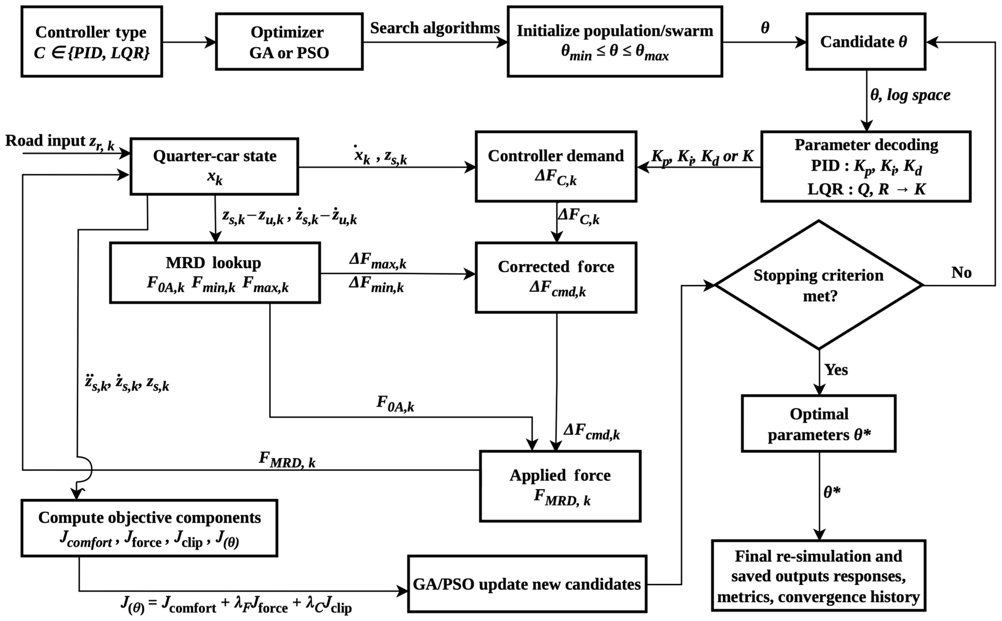
Figure 5 summarizes the common optimization workflow, in which each candidate is decoded into PID gains or LQR weighting parameters, evaluated through the force-constrained simulation on the composite B–C–D tuning road, and iteratively updated based on the resulting objective value until the stopping criterion is met. For each controller type, GA and PSO use the same predefined seed candidates within the logarithmic search domain, while the remaining population/swarm members are randomly initialized. In the repeated-run assessment, the optimizer random seed is varied while these predefined candidates and all other settings are retained unchanged.

4.5. Road Inputs and Evaluation Metrics

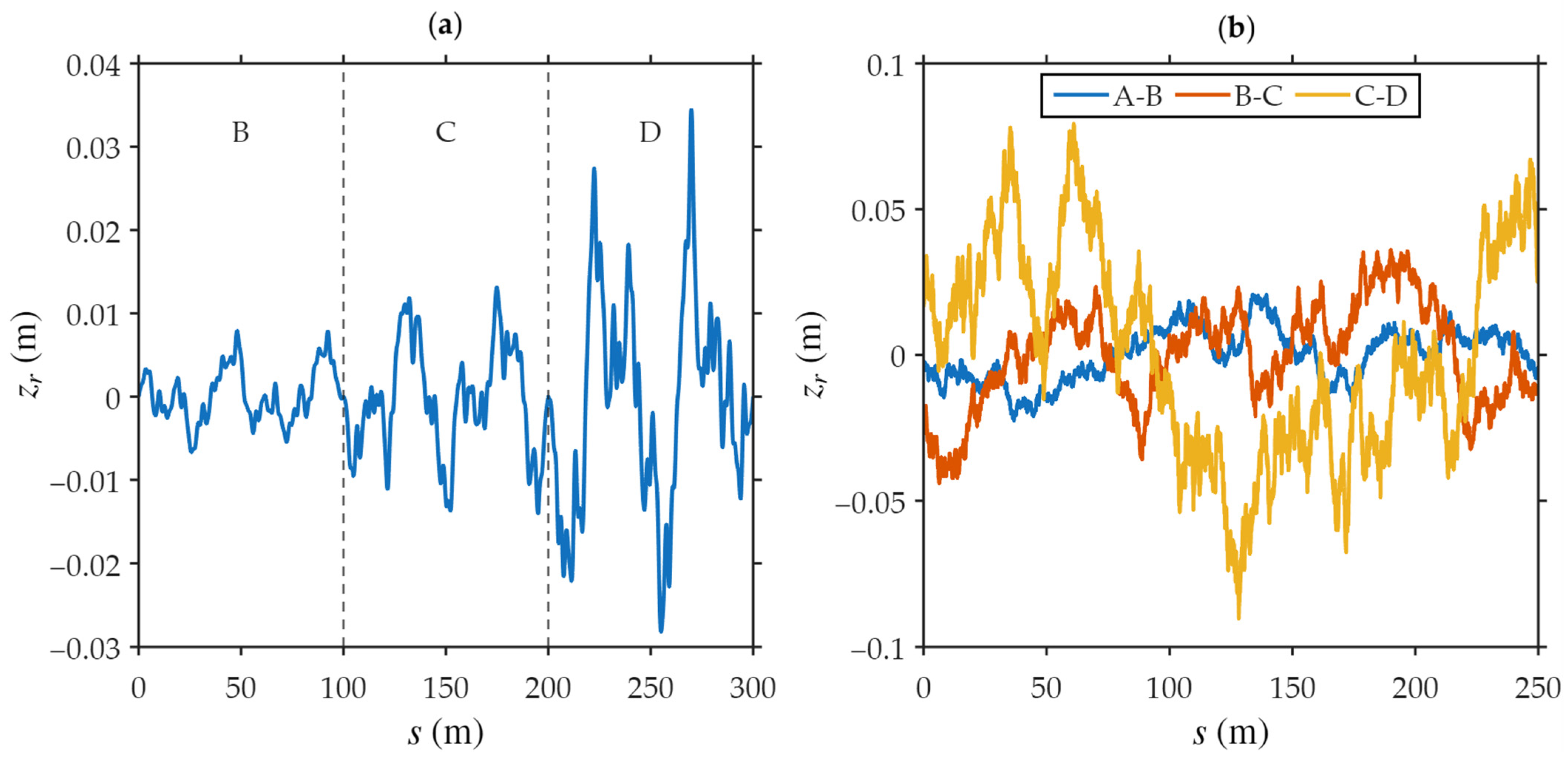
Two sets of road excitations were used for controller tuning and post-optimization robustness assessment. During optimization, each candidate controller was evaluated on a composite excitation consisting of three consecutive 100 m segments with increasing B-, C-, and D-level roughness. The total tuning distance was 300 m and the vehicle speed was fixed at 20 m/s. This multi-segment excitation exposes every candidate parameter set to successive changes in excitation severity within one objective evaluation.

After optimization, the four controller–optimizer combinations were evaluated over a cross-condition robustness matrix comprising three stochastic spatial road profiles, $\mathrm{A}\text{–}\mathrm{B},\mathrm{B}\text{–}\mathrm{C},\mathrm{C}\text{–}\mathrm{D}$, and three vehicle speeds, $v_x\in \{15,20,25\} \mathrm{m}/\mathrm{s}$.

This results in nine road–speed scenarios for each controller configuration. The spatial profiles used for robustness assessment are shown in Figure 6, while the complete tuning and evaluation conditions are summarized in

Table 5. Tuning and robustness evaluation scenarios.

Assessment Stage	Road Condition	Reference ${\mathit{G}}_{\mathit{d}}\left({\mathit{n}}_0\right)$	Road Length	Vehicle Speed
Optimization	Composite B–C–D	-	$3\times 100 \mathrm{m}$	$20 \mathrm{m}/\mathrm{s}$
Robustness	A–B	$32\times {10}^{-6} {\mathrm{m}}^3$	$250 \mathrm{m}$	$15, 20, 25 \mathrm{m}/\mathrm{s}$
Robustness	B–C	$128\times {10}^{-6} {\mathrm{m}}^3$	$250 \mathrm{m}$	$15, 20, 25 \mathrm{m}/\mathrm{s}$
Robustness	C–D	$512\times {10}^{-6} {\mathrm{m}}^3$	$250 \mathrm{m}$	$15, 20, 25 \mathrm{m}/\mathrm{s}$

.

The robustness road profiles are generated in the spatial domain using the power-spectral-density relation:

$$G_d(n)=G_d(n_0){\left({\displaystyle \frac{n}{n_0}}\right)}^{-w}$$

(44)

where $n_0=0.1 \mathrm{c}\mathrm{y}\mathrm{c}\mathrm{l}\mathrm{e}/\mathrm{m},w=2.$ The A–B, B–C, and C–D profiles are represented by the geometric midpoint PSD levels $G_d\left(n_0\right)=32\times {10}^{-6},128\times {10}^{-6},512\times {10}^{-6} {\mathrm{m}}^3,$ respectively. The spatial road elevation is synthesized as

$$z_r(s)={\displaystyle \sum _{q=1}^{N_h}}\sqrt{2G_d\left(n_q\right)\mathsf{\Delta }{n}_q}\mathrm{c}\mathrm{o}\mathrm{s}(2\pi n_{q}s+{\varphi }_q)$$

(45)

where $n_q$ is the $q$-th spatial frequency, $\mathsf{\Delta }{n}_q$ is the corresponding frequency increment, and ${\varphi }_q$ is a uniformly distributed random phase over $[0;2\pi ]$. In the present implementation $N_h=600,$ with spatial frequencies ranging from $n_{min}={\displaystyle \frac{1}{L}}$ to $n_{\mathrm{m}\mathrm{a}\mathrm{x}}={\displaystyle \frac{10 \mathrm{c}\mathrm{y}\mathrm{c}\mathrm{l}\mathrm{e}}{\mathrm{m}}},\mathsf{\Delta }s=0.02 \mathrm{m}.$ Each robustness profile has a length of $L = 250 \mathrm{m}$. The spatial road profile is converted to the time domain according to

$$s=v_{x}t,; z_r\left(t\right)=z_r\left(v_{x}t\right)$$

(46)

For each roughness level, the same spatial realization was retained across the three vehicle speeds. Therefore, changes in the dynamic response with speed were not affected by differences between stochastic road realizations. Fixed random seeds were used to ensure reproducibility of the generated profiles.

The dynamic response was evaluated using the RMS body acceleration, body velocity, and body displacement $RMS\left({\ddot{z}}_s\right),RMS\left({\dot{z}}_s\right),RMS\left(z_s\right)$ together with the RMS suspension travel and tire deflection $RMS\left(z_s-z_u\right),RMS(z_u-z_r)$.

For any response quantity $y$,

$$\mathrm{R}\mathrm{M}\mathrm{S}(y)=\sqrt{{\displaystyle \frac{1}{N}}{\displaystyle \sum _{k=1}^N}{y}_k^2}$$

(47)

while the corresponding peak metric is evaluated as

$$y_{\mathrm{p}\mathrm{e}\mathrm{a}\mathrm{k}}=\underset{k}{\mathrm{m}\mathrm{a}\mathrm{x}}\mid y_k\mid$$

(48)

Peak sprung-mass acceleration, suspension travel, and tire deflection are also reported to assess transient response severity. The actuator-feasibility assessment is based on the absolute force-deviation metric:

$$F_{\mathrm{v}\mathrm{i}\mathrm{o},k}=\left|\mathsf{\Delta }{F}_{C,k}-\mathsf{\Delta }{F}_{\mathrm{c}\mathrm{m}\mathrm{d},k}\right|$$

(49)

The root-mean-square force violation $\mathrm{R}\mathrm{M}\mathrm{S}\left(F_{\mathrm{v}\mathrm{i}\mathrm{o}}\right)$ is calculated as

$$\mathrm{R}\mathrm{M}\mathrm{S}(F_{\mathrm{v}\mathrm{i}\mathrm{o}})=\sqrt{{\displaystyle \frac{1}{N}}{\displaystyle \sum _{k=1}^N}{F}_{\mathrm{v}\mathrm{i}\mathrm{o},k}^2}$$

(50)

The corresponding clipping rate $r_{\mathrm{c}\mathrm{l}\mathrm{i}\mathrm{p}}$ is defined as

$$r_{\mathrm{c}\mathrm{l}\mathrm{i}\mathrm{p}}={\displaystyle \frac{1}{N}}{\displaystyle \sum _{k=1}^N}{c}_k$$

(51)

where $c_k$ is defined in Equation (34). These physical diagnostics are reported separately from the normalized objective-function terms $J_{\mathrm{f}\mathrm{o}\mathrm{r}\mathrm{c}\mathrm{e}}$ and $J_{\mathrm{c}\mathrm{l}\mathrm{i}\mathrm{p}}$. Performance improvement relative to the passive zero-current MRD configuration is calculated as

$$J_M=100\left(1−{\displaystyle \frac{M_{\mathrm{c}\mathrm{t}\mathrm{r}\mathrm{l}}}{M_{0A}}}\right)$$

(52)

where $M_{\mathrm{c}\mathrm{t}\mathrm{r}\mathrm{l}}$ and $M_{0A}$ denote the same response metric for the semi-active controller and the passive 0 A reference, respectively. A positive value of $J_M$ therefore indicates an improvement relative to the passive 0 A MRD baseline.

5. Results and Discussion

5.1. Optimization Results

The optimization results are examined from four complementary perspectives. First, the convergence histories indicate how GA and PSO explore the PID and LQR parameter spaces. Second, the representative optimized parameter sets are examined together with their final objective values. Third, repeated independent runs are used to quantify stochastic repeatability and parameter-space variability. Finally, the objective function is decomposed into comfort, force-feasibility, and clipping contributions to clarify the trade-off underlying the optimized solutions.

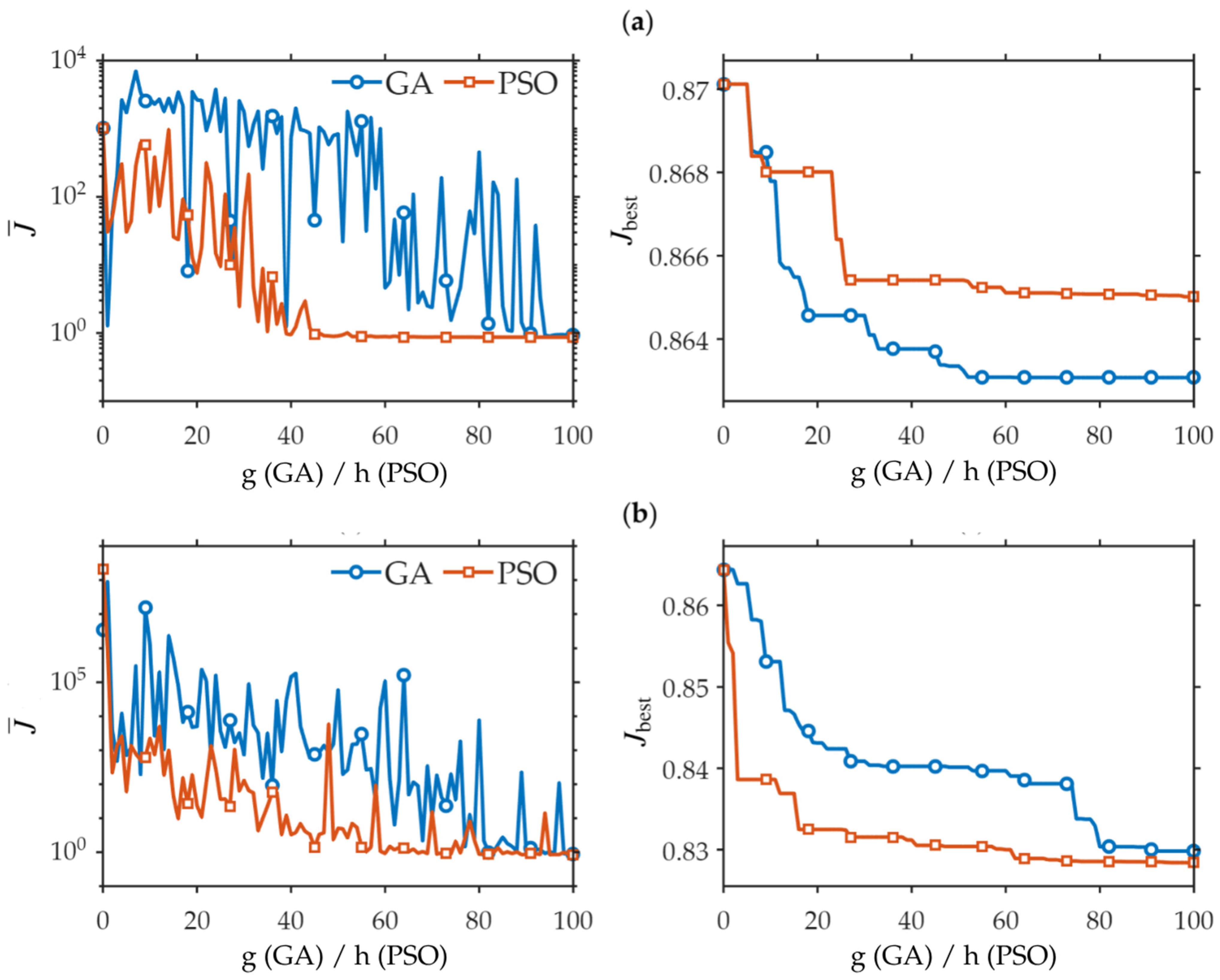
Figure 7 and

Table 6. Representative optimized controller parameters used for the detailed dynamic-response and cross-condition analyses.

Model	Optimized Parameters	Jopt
PID-GA	$K_p=974.067;K_i=2781.039;K_d=0.016559$	0.863074
PID-PSO	$K_p=1168.887;Ki=705.545;K_d=0.011855$	0.865013
LQR-GA	$Q=diag\left(\mathrm{282,412},\mathrm{10,761}, \mathrm{746,125},4.39767\times {10}^{-4}\right);$ $R=1.38924\times {10}^{-2}$; $K=\left[-594.087,-1084.840,512.285,106.053\right]$	0.829825
LQR-PSO	$Q=diag\left(1.14276\times {10}^4,77.8326,1.7163\times {10}^{-7},9.35370\right);$ $R=1.87859\times {10}^{-4}$; $K=\left[-1721.061,-1244.304,838.456,202.036\right]$	0.828389

summarize the optimization behavior and the final parameter sets. The convergence histories compare GA and PSO under the same candidate evaluation procedure, while the optimized parameters show whether similar objective values require similar controller settings.

For the representative solutions used in the subsequent detailed analyses, PID-GA and PID-PSO achieve objective values of 0.863074 and 0.865013, respectively, while LQR-GA and LQR-PSO achieve 0.829825 and 0.828389. These representative solutions are retained for the time-domain, force-feasibility, and cross-condition analyses, while their sensitivity to stochastic optimizer initialization is assessed separately through the repeated-run analysis described below.

The convergence histories in Figure 7 show rapid early improvement followed by gradual refinement. The mean objective exhibits larger fluctuations than the best-so-far objective because the population or swarm continues to explore candidates with different dynamic-response and force-feasibility characteristics. The convergence histories are therefore used to illustrate the search behavior of the representative runs, whereas the optimization repeatability of the small terminal differences is examined using the five-run results reported below.

The optimized PID gains and LQR weighting parameters are reported in Table 6. None of the final solutions reach the imposed search bounds, indicating that the reported solutions are not directly truncated by the selected parameter limits.

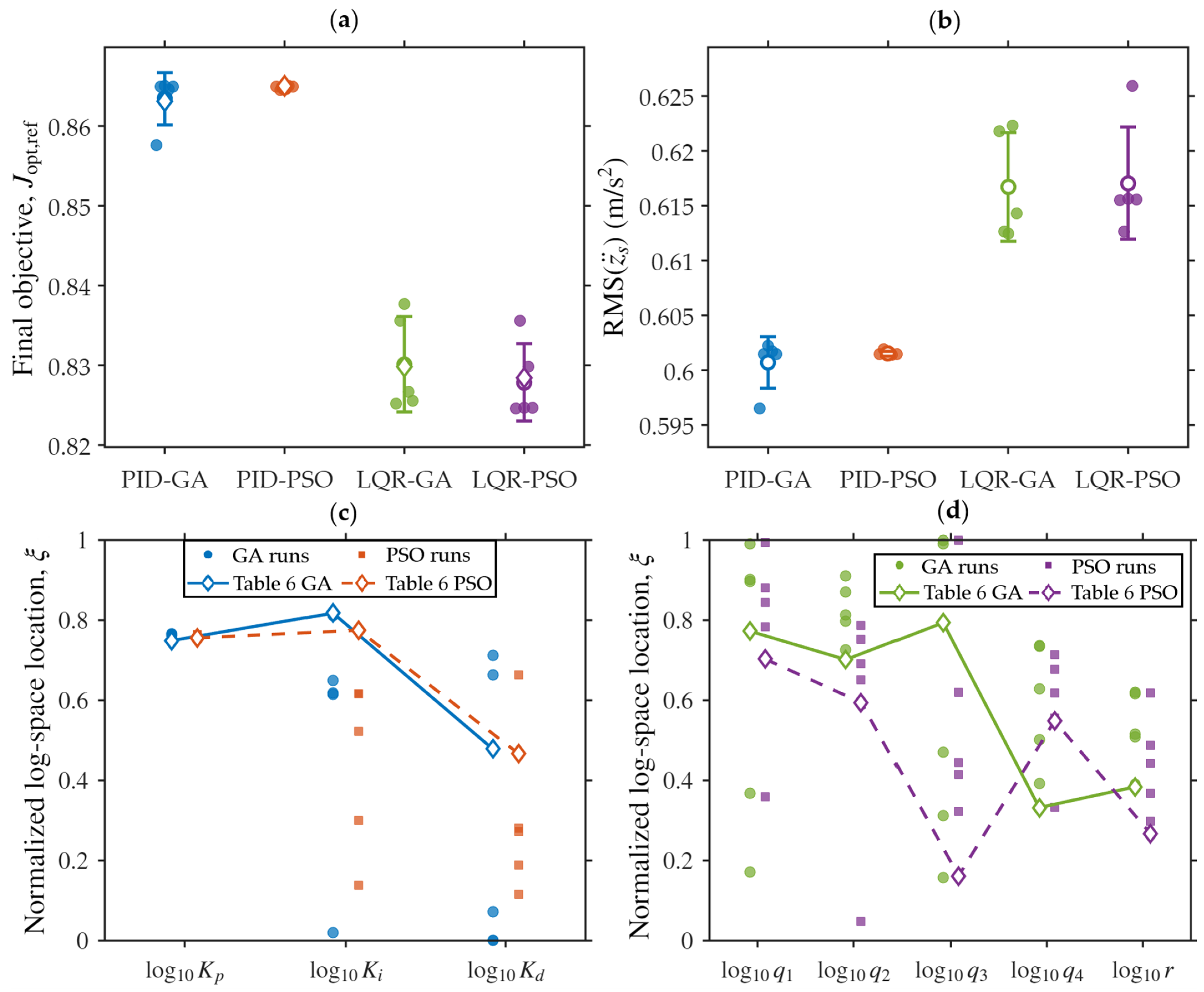
To quantify stochastic repeatability, testing of each controller–optimizer configuration was independently repeated five times using different optimizer seeds under otherwise identical conditions.

Table 7. Statistical summary over five independent optimization runs. Values are reported as mean ± standard deviation.

Model	Jopt,ref	RMS ${\ddot{\mathit{z}}}_{\mathit{s}}$ (m/s2)	RMS ${\dot{\mathit{z}}}_{\mathit{s}}$ (m/s)	RMS ${\mathit{z}}_{\mathit{s}}$ (m)	RMS ${\mathit{z}}_{\mathit{s}}-{\mathit{z}}_{\mathit{u}}$ (m)	RMS ${\mathit{z}}_{\mathit{u}}-{\mathit{z}}_{\mathit{r}}$ (m)	${\mathit{J}}_{\mathit{F}}$	Clip Rate	RMS Force Violation (N)
PID-GA	0.863419 ± 0.003257	0.600680 ± 0.002349	0.048728 ± 0.000801	0.009389 ± 0.000206	0.007080 ± 0.000111	0.002185 ± 0.000012	0.028240 ± 0.002049	0.419793 ± 0.005281	41.044 ± 2.082
PID-PSO	0.864884 ± 0.000215	0.601520 ± 0.000216	0.048982 ± 0.000226	0.009468 ± 0.000035	0.007120 ± 0.000030	0.002179 ± 0.000004	0.027669 ± 0.000883	0.417861 ± 0.002260	40.238 ± 0.084
LQR-GA	0.830130 ± 0.006003	0.616697 ± 0.004948	0.048711 ± 0.000540	0.009281 ± 0.000285	0.006812 ± 0.000234	0.002091 ± 0.000014	0.011936 ± 0.001412	0.308231 ± 0.029709	25.295 ± 2.167
LQR-PSO	0.827859 ± 0.004858	0.617046 ± 0.005121	0.048530 ± 0.000769	0.009164 ± 0.000237	0.006730 ± 0.000189	0.002092 ± 0.000010	0.012525 ± 0.001625	0.305298 ± 0.021930	25.367 ± 1.641

summarizes the resulting mean ± standard-deviation statistics. For direct comparison with the representative objective values in Table 6, the repeated-run objective values are reported, while all physical response and force-feasibility metrics are reported directly from the simulations. Figure 8a,b present the corresponding individual-run distributions of the objective value and RMS sprung-mass acceleration. For the parameter-space visualization in Figure 8c,d, each logarithmic parameter coordinate is normalized to its corresponding search interval in Table 3 as ${\xi }_j=({\theta }_j-L_j)/(U_j-L_j)$, where ${\theta }_j={log}_{10}\left(p_j\right)$, and $L_j$ and $U_j$ denote the lower and upper logarithmic bounds, respectively. These original fixed-seed optimized solutions are retained as the representative cases for the subsequent time-domain, force-feasibility, and cross-condition analyses, while the five additional runs are used separately to quantify stochastic repeatability.

The mean objective values are 0.863419 ± 0.003257, 0.864884 ± 0.000215, 0.830130 ± 0.006003, and 0.827859 ± 0.004858 for PID-GA, PID-PSO, LQR-GA, and LQR-PSO, respectively. The coefficients of variation remain below approximately 0.73% for the objective value and below 0.83% for RMS sprung-mass acceleration. PID-PSO exhibits particularly low run-to-run variability, whereas the LQR-based searches show somewhat greater sensitivity to stochastic initialization.

The mean GA–PSO differences are approximately 0.17% for PID and 0.27% for LQR and remain small relative to the observed stochastic dispersion. These results therefore support a configuration-dependent interpretation rather than universal superiority of either optimizer.

The repeated optimizations also reveal substantial parameter non-uniqueness. As shown in Figure 8c,d, the PID proportional gain remains relatively concentrated, whereas the integral and derivative gains can occupy widely separated regions of the logarithmic search space while producing comparable objective and response values. The LQR weighting parameters exhibit even broader distributions across the admissible domains.

For PID, this behavior reflects compensation among the proportional, integral, and derivative contributions. For LQR, the weighting parameters are inherently relative, and a common positive scaling of Q and R leaves the continuous-time feedback gain unchanged. A further source of non-uniqueness arises from the common semi-active force-realization mechanism, through which different unconstrained controller demands may be projected onto similar experimentally attainable MRD forces. Consequently, similar closed-loop performance does not require a unique controller parameter vector, and the resulting solutions are interpreted as different near-optimal parameterizations rather than as a uniquely identifiable optimum.

Because of this parameter non-uniqueness, the optimized gains and weighting coefficients are treated as representative near-optimal designs rather than uniquely identifiable controller parameters. The representative parameter sets in Table 6 are therefore retained for the subsequent detailed analyses rather than replacing them with averaged values across the repeated runs, since an averaged parameter vector would not itself represent an independently optimized controller.

The relatively small dispersion of the repeated-run performance metrics indicates that different parameter combinations can lie within a similar near-optimal performance region. However, this parameter non-uniqueness does not imply identical robustness of all such solutions under changing operating conditions. Therefore, the representative solutions in Table 6 are subsequently assessed over the nine-scenario cross-condition road–speed matrix in Section 5.3.

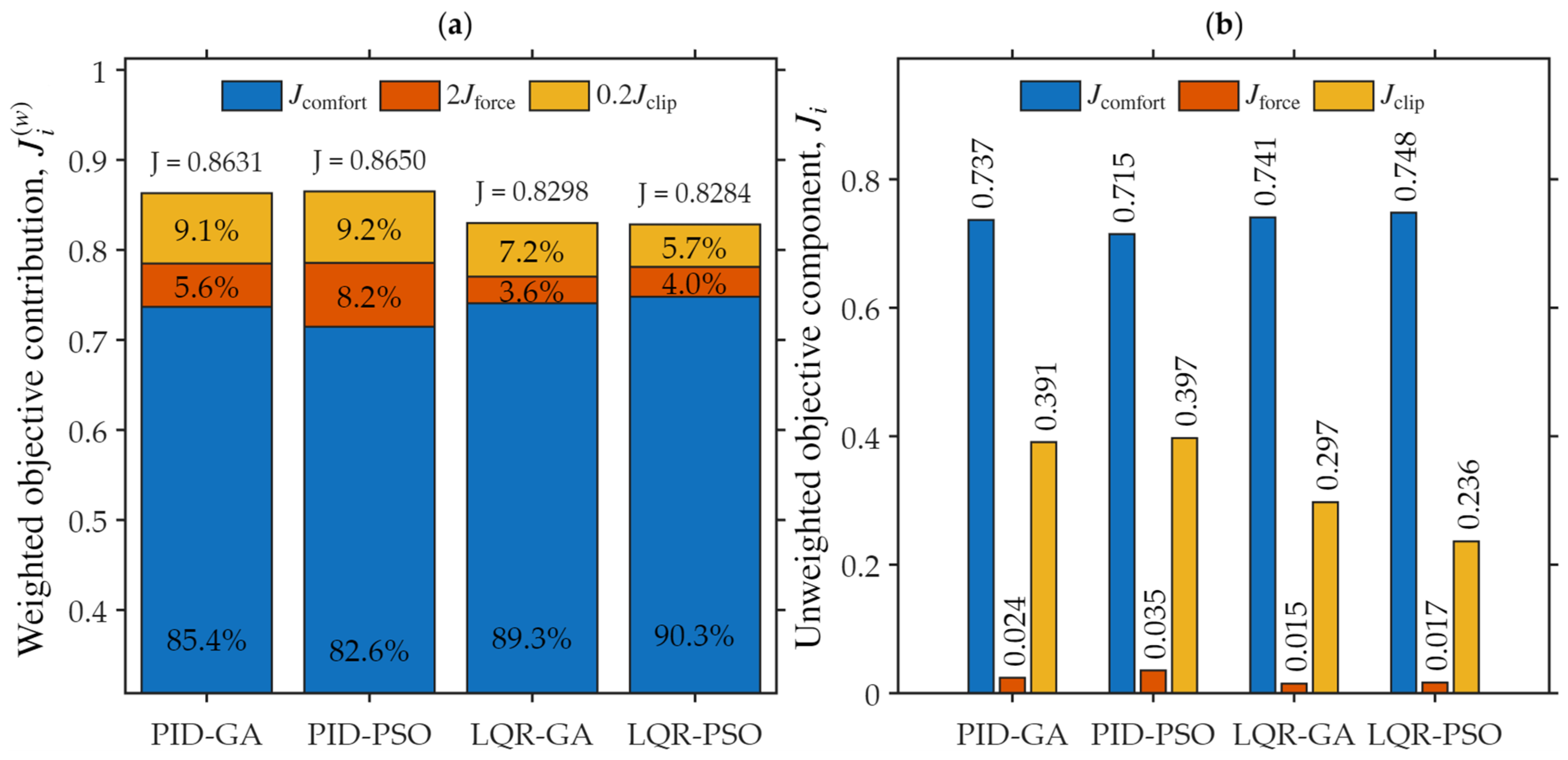
The objective-function decomposition in Figure 9 confirms the same trade-off. PID-PSO provides the strongest comfort-oriented optimization outcome, LQR-GA gives the lowest normalized force-feasibility penalty, and LQR-PSO gives the lowest clipping component and the lowest total objective. The weighted contributions in Figure 9a show how these terms combine in the final objective value, whereas Figure 9b presents the corresponding unweighted components. The optimum is therefore governed by the balance between vibration reduction and compatibility with the experimental MRD force range.

5.2. Dynamic Response Comparison

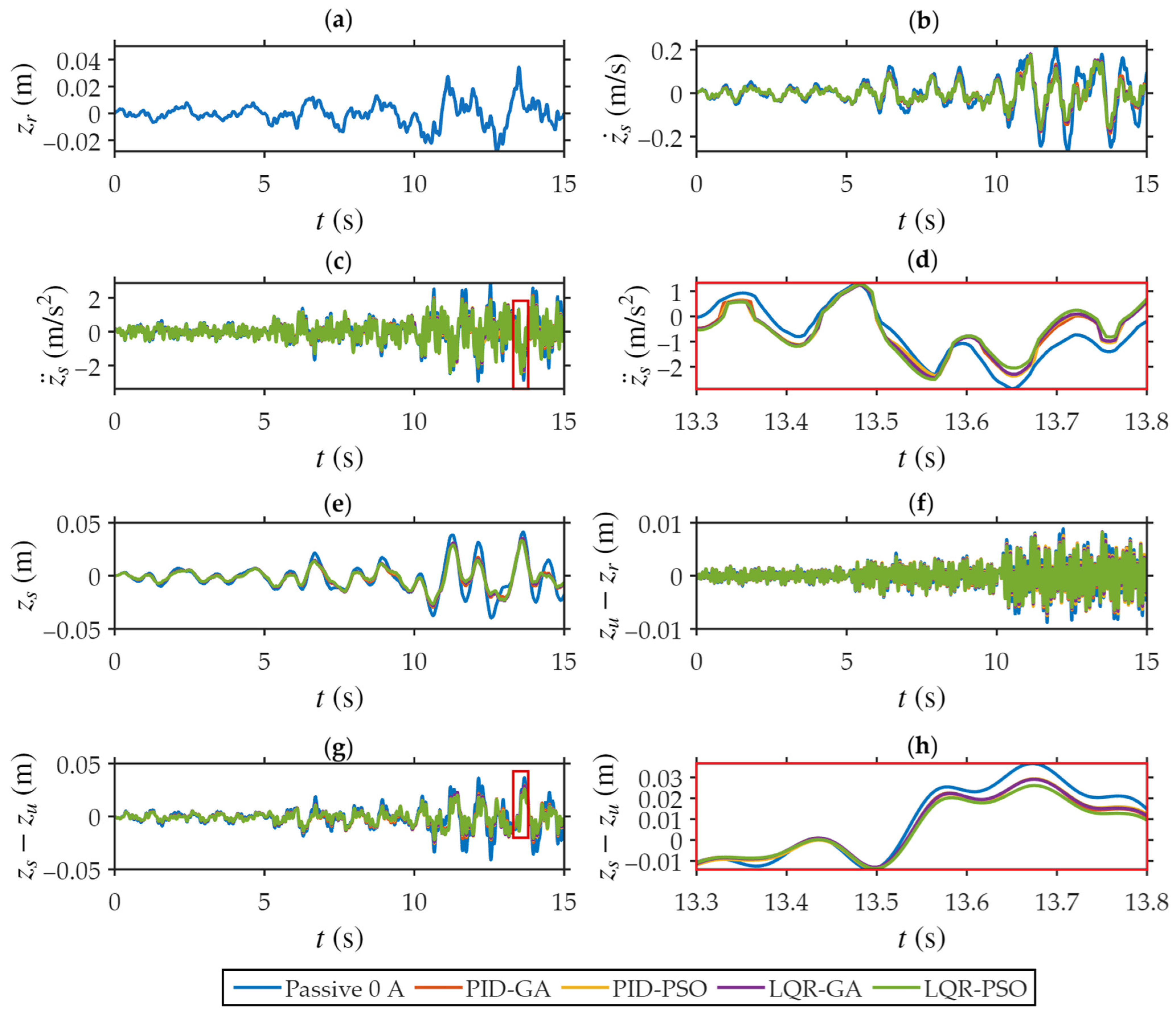
Figure 10 and

Table 8. Main-scenario dynamic performance of the passive and optimized semi-active suspensions.

Model	RMS ${\ddot{\mathit{z}}}_{\mathit{s}}$ (m/s2)	RMS ${\dot{\mathit{z}}}_{\mathit{s}}$ (m/s)	RMS ${\mathit{z}}_{\mathit{s}}$ (m)	RMS ${\mathit{z}}_{\mathit{s}}-{\mathit{z}}_{\mathit{u}}$ (m)	Peak $\mid {\ddot{\mathit{z}}}_{\mathit{s}}\mid$ (m/s2)
Passive	0.722845	0.080701	0.013828	0.010642	2.932854
PID-GA	0.621174 (−14.07%)	0.054587 (−32.36%)	0.010255 (−25.83%)	0.007406 (−30.41%)	2.480423 (−15.43%)
PID-PSO	0.607854 (−15.91%)	0.052467 (−34.99%)	0.010274 (−25.70%)	0.007428 (−30.20%)	2.371138 (−19.15%)
LQR-GA	0.621561 (−14.01%)	0.053139 (−34.15%)	0.010330 (−25.29%)	0.007331 (−31.12%)	2.452864 (−16.37%)
LQR-PSO	0.632276 (−12.53%)	0.050286 (−37.69%)	0.009673 (−30.05%)	0.006732 (−36.75%)	2.504833 (−14.59%)

compare the passive zero-current MRD baseline with the four optimized semi-active configurations under the composite B–C–D tuning excitation at 20 m/s. All optimized controllers reduce the principal body-response measures, but their response priorities are different.

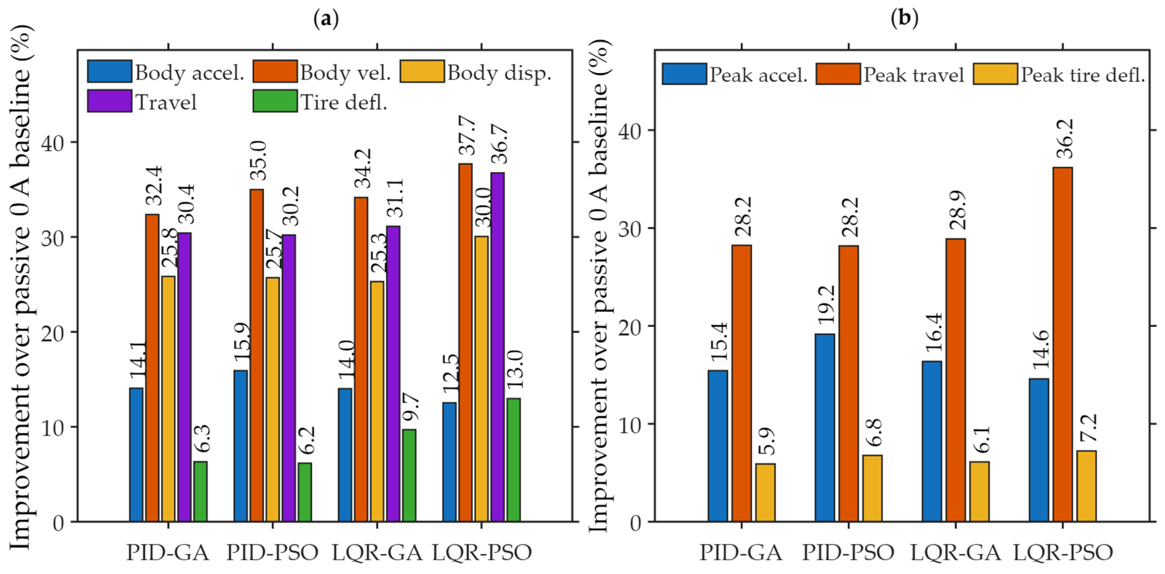
For the representative optimized solutions, PID-PSO provides the strongest acceleration-oriented performance, reducing RMS sprung-mass acceleration from 0.722845 to 0.607854 m/s² (15.91%) and peak acceleration by 19.15% relative to the passive baseline. LQR-PSO provides broader body-motion and suspension regulation. It reduces RMS sprung-mass velocity by 37.69%, body displacement by 30.05%, and suspension travel by 36.75%. The time histories confirm that this attenuation is maintained over the complete tuning excitation.

Within the four configurations considered in the present framework, the tuning scenario reveals two distinct control tendencies: PID-PSO favors sprung-mass acceleration attenuation, whereas LQR-PSO provides a broader balance between body-motion reduction and suspension regulation.

Figure 11 provides a compact quantitative summary of the same tuning-condition results. The RMS improvements in Figure 11a highlight the stronger acceleration reduction in PID-PSO and the broader reductions in body velocity, body displacement, and suspension travel achieved by LQR-PSO. The peak-response improvements in Figure 11b further show that the controller ranking depends on the response quantity considered. Together with the time histories in Figure 10 and the values in Table 8, these results confirm distinct controller priorities and motivate the subsequent force-feasibility and cross-condition assessment.

5.3. Force Feasibility and Robustness Assessment

The four optimized controllers are next evaluated from two complementary perspectives: compatibility of the desired correction force with the experimental MRD force range, and robustness over the nine-case cross-condition road–speed matrix.

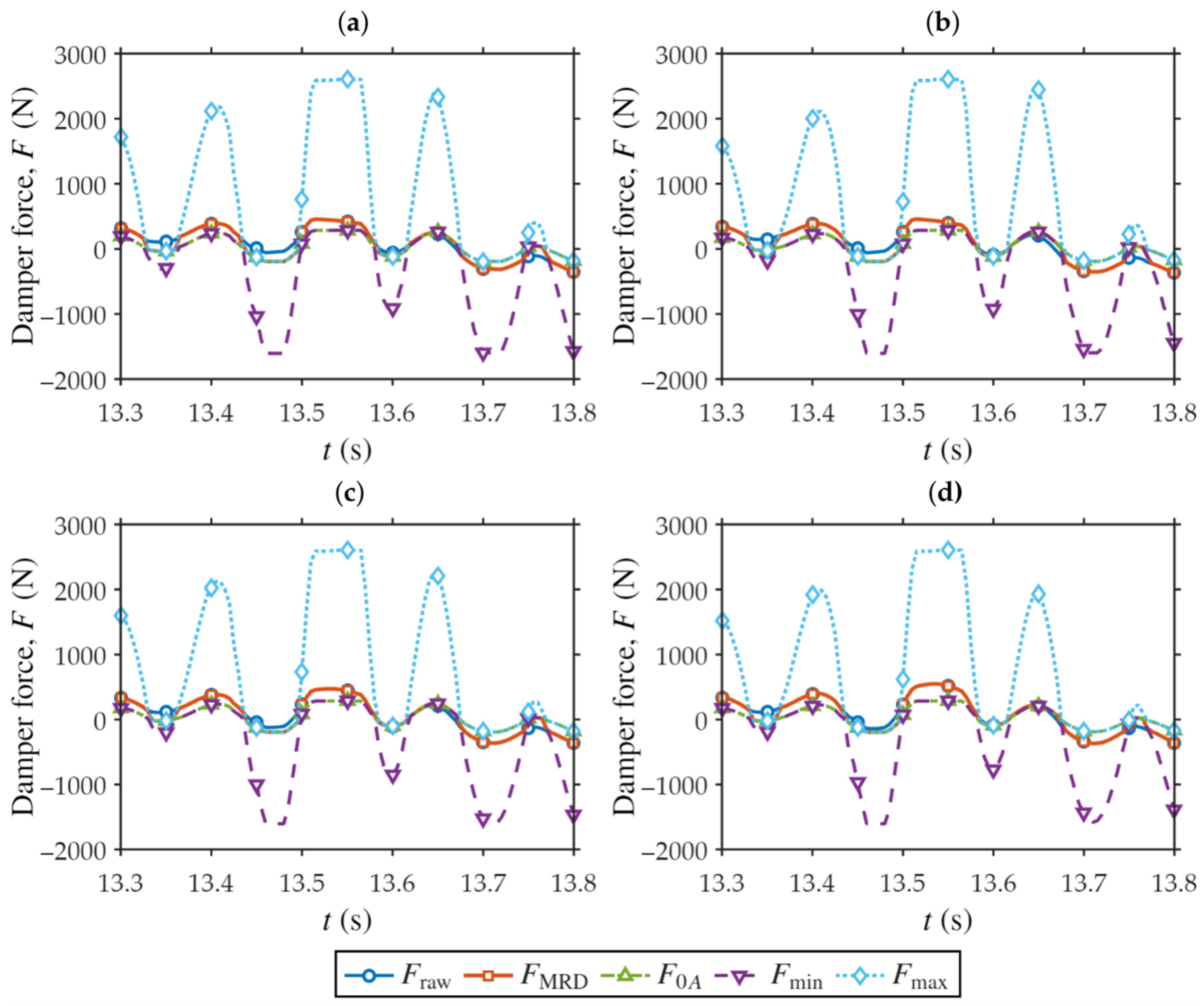
Figure 12 compares the desired total force behavior with the applied MRD force, the zero-current baseline, and the experimentally supported force limits for the four optimized configurations. The applied force remains inside the feasible envelope because the desired correction force is limited according to Section 4.3. The difference between the requested and feasible correction forces is therefore reflected in the force-violation and clipping metrics summarized in

Table 9. Force-feasibility metrics of the optimized semi-active controllers under the composite B–C–D tuning excitation.

Model	RMS Force Violation (N)	Jforce	Clip Rate (-)	Jopt
PID-GA	30.715	0.024081	0.390870	0.863074
PID-PSO	33.717	0.035469	0.397201	0.865013
LQR-GA	22.801	0.014847	0.297234	0.829825
LQR-PSO	20.622	0.016550	0.236255	0.828389

.

PID-PSO gives the strongest acceleration reduction in the tuning scenario but also the largest absolute force violation (33.717N RMS) and the highest clipping rate (0.397201). LQR-PSO gives the lowest absolute force violation (20.622N RMS) and clipping rate (0.236255), while LQR-GA gives the lowest normalized force-feasibility component. These results demonstrate that maximum vibration attenuation and force feasibility are not identical design objectives.

The force-feasibility comparison therefore supports the trade-off observed in the tuning responses and provides a physical interpretation of the objective-function ranking.

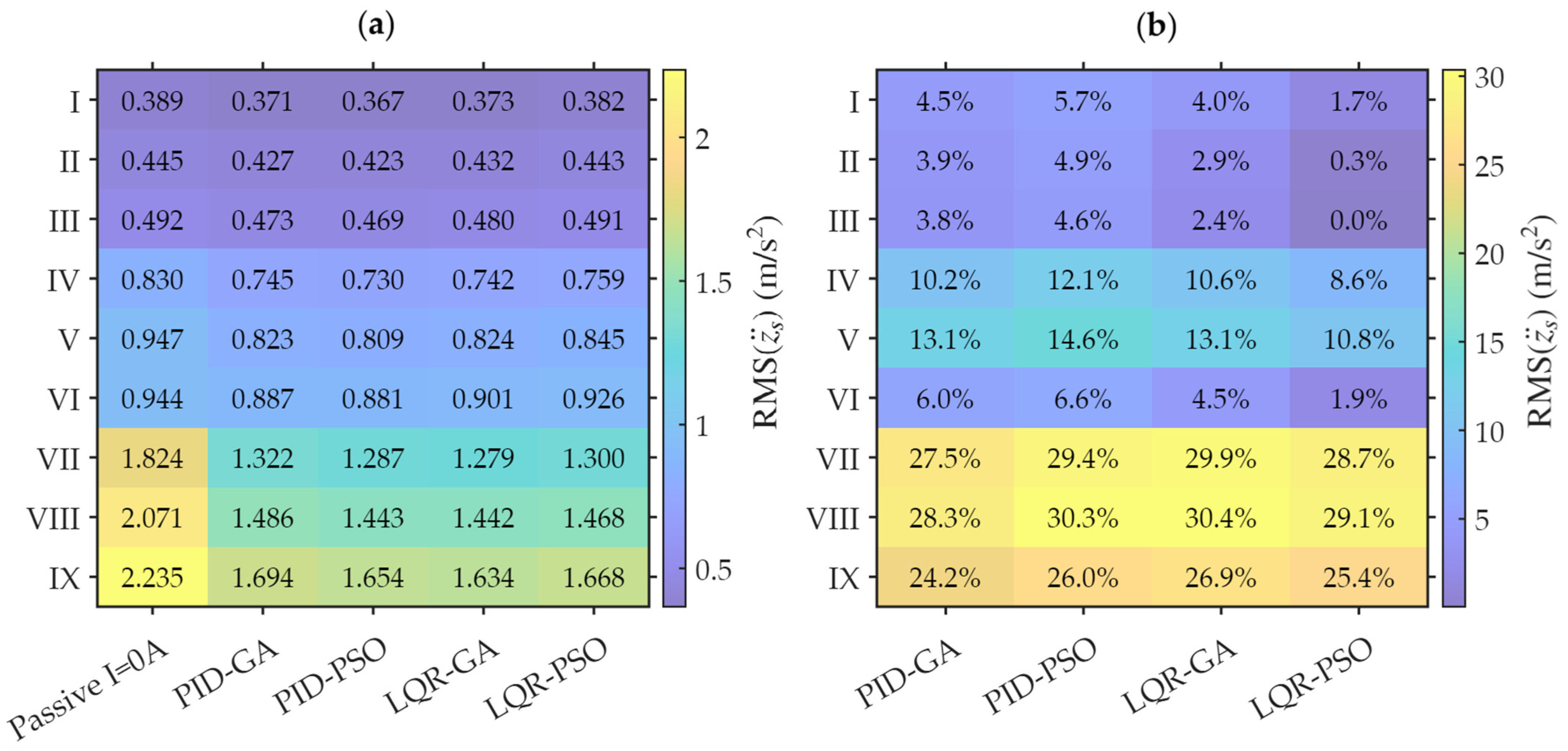
Figure 13 presents the RMS sprung-mass acceleration and its reduction relative to the passive baseline over the nine evaluated road–speed scenarios.

PID-PSO produces the lowest RMS sprung-mass acceleration in all six A–B and B–C scenarios, whereas LQR-GA gives the lowest values in all three C–D scenarios. The acceleration-oriented ranking therefore changes with excitation severity.

This result shows why the tuning condition alone cannot establish controller superiority over a wider operating domain: the composite road identifies the controller parameters, whereas the cross-condition matrix reveals how the optimized solutions respond to changes in roughness and speed.

The aggregate statistics in

Table 10. Cross-scenario performance across road-profile roughness levels and vehicle speeds.

Model	Mean ΔRMS ${\ddot{\mathit{z}}}_{\mathit{s}}$ (%)	Mean ΔRMS ${\dot{\mathit{z}}}_{\mathit{s}}$ (%)	Mean ΔRMS Travel (%)	Mean ΔRMS Tire Deflection (%)	Worst RMS ${\ddot{\mathit{z}}}_{\mathit{s}}$	Mean Clip Rate	Mean RMS Force Violation (N)	Best RMS Accel. Cases
PID-GA	13.51	33.44	28.38	9.94	1.6945	0.4210	48.28	0/9
PID-PSO	14.91	35.33	28.42	10.23	1.6538	0.4197	49.73	6/9
LQR-GA	13.84	35.99	31.29	16.62	1.6336	0.2930	30.88	3/9
LQR-PSO	11.83	39.45	36.73	21.79	1.6679	0.2396	28.43	0/9

show that PID-PSO achieves the largest mean RMS acceleration improvement and is best in six of the nine acceleration cases. LQR-GA gives the lowest worst-case RMS acceleration and is best in the three severe C–D cases. LQR-PSO provides the broadest overall behavior, with the largest mean reductions in sprung-mass velocity, suspension travel, and tire deflection, together with the lowest mean clipping rate and mean RMS force violation.

Overall, the four configurations exhibit complementary performance priorities within the present controlled comparison. PID-PSO favors acceleration attenuation, whereas LQR-PSO provides a broader balance among body motion, suspension working space, tire response, and MRD force feasibility. These results show that controller and optimizer selection influences the resulting performance trade-off rather than defining a single configuration that is preferable for all operating objectives.

6. Conclusions

This study developed an experimentally constrained optimization framework for MRD-based semi-active suspension control. A branch-dependent lookup model derived from measured damper characteristics was used to provide the zero-current baseline force and instantaneous feasible force envelope. This envelope was enforced at every simulation step and during every GA and PSO fitness evaluation, so that controller optimization was performed using the force-constrained semi-active response rather than an unconstrained active-force model. The main conclusions are as follows.

• The common comparison framework provides a consistent basis for comparing controller structure and optimizer selection. PID and LQR controllers were independently tuned by GA and PSO under the same plant model, objective function, tuning excitation, search domain, and force constraints. Across the repeated optimization runs, GA retains a slightly lower mean objective for PID, whereas PSO retains a slightly lower mean objective for LQR. However, these differences are small relative to the observed stochastic variability, confirming that no universal optimizer superiority can be inferred from the present comparison.
• The optimized controllers exhibited different performance priorities. PID-PSO provided the strongest acceleration-oriented response, whereas LQR-PSO achieved the best overall balance among body-motion suppression, suspension travel, tire response, and force feasibility. Thus, maximum vibration attenuation does not necessarily correspond to the most compatible demand with the experimentally supported MRD force envelope.
• The nine-scenario assessment showed that controller ranking varies across the evaluated road–speed conditions. PID-PSO performed best in most acceleration-oriented cases, whereas LQR-based solutions became more competitive under the severe road cases considered. LQR-PSO provided the most balanced performance across the evaluated scenarios.

Overall, the results indicate that the four controller–optimizer configurations provide different trade-offs among vibration attenuation, suspension response, and compatibility with the experimentally supported MRD force range. Their relative suitability therefore depends on the prioritized performance objective and operating condition, consistent with the controlled comparative purpose of the present framework. Within this scope, the present work provides a concept-level, force-command-based evaluation using a linear quarter-car model and offline optimization. The experimental MRD characterization supplies the measured force data and attainable operating envelope used throughout the controller evaluation, providing the experimental basis for the proposed constrained framework. Closed-loop implementation of the optimized controllers with the physical MR damper represents the next stage toward practical validation, including inverse force-to-current realization, current-driver dynamics, sensing, and real-time control. The current framework also employs prescribed optimization settings and objective-function weights, focuses on the controlled PID/LQR-GA/PSO comparison, and adopts full-state feedback for the LQR formulation. Building on these results, future work will investigate sensitivity to optimization settings and objective weights, closed-loop bench validation, extension to higher-order vehicle models, and broader comparisons with other semi-active control strategies, including Skyhook and MPC, under the same experimentally constrained MRD framework.

References

1. Yu, M.; Evangelou, S.A.; Dini, D. Advances in Active Suspension Systems for Road Vehicles. Engineering 2024, 33, 160–177. [Google Scholar] [CrossRef] [Scilit]
2. Wu, X.; Pan, Y.; Wang, G.; Hou, L. Pitch Motion Suppression of Electric Vehicle Active Suspensions Based on Multibody Dynamics. Mech. Mach. Theory 2024, 198, 105667. [Google Scholar] [CrossRef] [Scilit]
3. Tapia, P.; Tramacere, E.; Puma-Benavides, D.S.; Galluzzi, R.; Zambrano-Leon, V.D.; Jima-Matailo, J.C.; Llanes-Cedeño, E.A. Comparative Analysis of MacPherson and Double Wishbone Suspensions for an Electric Off-Road Vehicle Retrofit. World Electr. Veh. J. 2025, 16, 228. [Google Scholar] [CrossRef] [Scilit]
4. Skrickij, V.; Kojis, P.; Šabanovič, E.; Shyrokau, B.; Ivanov, V. Review of Integrated Chassis Control Techniques for Automated Ground Vehicles. Sensors 2024, 24, 600. [Google Scholar] [CrossRef] [Scilit] [PubMed]
5. Theunissen, J.; Tota, A.; Gruber, P.; Dhaens, M.; Sorniotti, A. Preview-Based Techniques for Vehicle Suspension Control: A State-of-the-Art Review. Annu. Rev. Control 2021, 51, 206–235. [Google Scholar] [CrossRef] [Scilit]
6. Ferhath, A.A.; Kasi, K. The Evolution of Damper Technology for Enhanced Ride Comfort and Vehicle Handling in Vehicle Suspension System. Int. J. Dyn. Control 2024, 12, 3908–3946. [Google Scholar] [CrossRef] [Scilit]
7. Ferhath, A.A.; Kasi, K. Orifice and Fluid Flow Modifications for Improved Damping in Vehicle Suspensions: A Comprehensive Review. J. Vib. Eng. Technol. 2024, 12, 6777–6808. [Google Scholar] [CrossRef] [Scilit]
8. Kim, J.; Lee, T.; Kim, C.-J.; Yi, K. Model Predictive Control of a Semi-Active Suspension with a Shift Delay Compensation Using Preview Road Information. Control Eng. Pract. 2023, 137, 105584. [Google Scholar] [CrossRef] [Scilit]
9. Li, G.; Gan, Y.; Liu, Q.; Xu, H.; Chen, D.; Zhong, L.; Deng, J.; Hu, G. Performance Analysis of Vehicle Magnetorheological Semi-Active Air Suspension Based on S-QFSMC Control. Front. Mater. 2024, 11, 1358319. [Google Scholar] [CrossRef] [Scilit]
10. Fathi, H.; El-Sayegh, Z.; Ren, J.; El-Gindy, M. Analysis of Tire-Road Interaction: A Literature Review. Machines 2024, 12, 812. [Google Scholar] [CrossRef] [Scilit]
11. Wang, Z.; Liu, C.; Zheng, X.; Zhao, L.; Qiu, Y. Advancements in Semi-Active Automotive Suspension Systems with Magnetorheological Dampers: A Review. Appl. Sci. 2024, 14, 7866. [Google Scholar] [CrossRef] [Scilit]
12. Qian, R.; Wang, G.; Jiang, M.; Zhang, Y.; Zhai, R.; Wang, W. Frequency-Dependent Bouc–Wen Modeling of Magnetorheological Damper Using Harmonic Balance Approach. Actuators 2024, 13, 297. [Google Scholar] [CrossRef] [Scilit]
13. Mohd Saufi, M.S.R.; Asrar Bin Ahmad, Z.; Firdaus Isham, M.; Hussin Ab Talib, M. Magnetorheological Damper Modelling with a Non-Parametric Approach of One-Dimensional LSTM and Differential Evolution. Mech. Time-Depend. Mater. 2026, 30, 30. [Google Scholar] [CrossRef] [Scilit]
14. Ali, S.A.; Metered, H.; Bassiuny, A.M.; Abdel-Ghany, A.M. Ride Comfort Enhancement of Railway Vehicles Using Magnetorheological Damper; Paper No. 2024-01-2291; SAE International: Detroit, MI, USA, 2024. [Google Scholar]
15. Zhang, Y.; Guo, J.; Yang, J.; Li, X. Recent Structural Developments and Applications of Magnetorheological Dampers (MRD): A Review. Magnetochemistry 2023, 9, 90. [Google Scholar] [CrossRef] [Scilit]
16. Hu, T.; Jiang, L.; Pan, L.; Chen, B.; Gong, N.; Yang, J.; Gong, X.; Sun, S. Development of a Semi-Active Suspension Using a Compact Magnetorheological Damper with Negative-Stiffness Components. Mech. Syst. Signal Process. 2025, 223, 111842. [Google Scholar] [CrossRef] [Scilit]
17. Hu, G.; Ying, S.; Qi, H.; Yu, L.; Li, G. Design, Analysis and Optimization of a Hybrid Fluid Flow Magnetorheological Damper Based on Multiphysics Coupling Model. Mech. Syst. Signal Process. 2023, 205, 110877. [Google Scholar] [CrossRef] [Scilit]
18. Jiang, M.; Rui, X.; Yang, F.; Zhu, W.; Zhang, Y. Multi-Objective Optimization Design for a Magnetorheological Damper. J. Intell. Mater. Syst. Struct. 2022, 33, 33–45. [Google Scholar] [CrossRef] [Scilit]
19. Lei, B.; Li, J.; Zhou, W.; Shou, M.; Zhao, F.; Liao, C. Dual-Stage Theoretical Model of Magnetorheological Dampers and Experimental Verification. Smart Mater. Struct. 2024, 33, 045027. [Google Scholar] [CrossRef] [Scilit]
20. Chen, C.; Ma, R.; Ma, W. GA-LQR for Vehicle Semi-Active Suspension with BiLSTM Inverse Model of Magnetic Rheological Damper. Trans. Can. Soc. Mech. Eng. 2023, 47, 423–435. [Google Scholar] [CrossRef] [Scilit]
21. Krauze, P. Identification of Control-Related Signal Path for Semi-Active Vehicle Suspension with Magnetorheological Dampers. Sensors 2023, 23, 5770. [Google Scholar] [CrossRef] [Scilit] [PubMed]
22. Jin, L.; Fan, J.; Du, F.; Zhan, M. Research on Two-Stage Semi-Active ISD Suspension Based on Improved Fuzzy Neural Network PID Control. Sensors 2023, 23, 8388. [Google Scholar] [CrossRef] [Scilit] [PubMed]
23. Ji, G.; Zhang, L.; Cai, M.; Meng, X.; Du, Z.; Ruan, J.; Guan, S.; Liu, Z. Research on Variable Universe Fuzzy PID Control for Semi-Active Suspension with CDC Dampers Based on Dynamic Adjustment Functions. Sci. Rep. 2024, 14, 3442. [Google Scholar] [CrossRef] [Scilit] [PubMed]
24. Ram, S.S.; Kumar, C.; Saravanakumar, R.; Banjerdpongchai, D. System Identification and Robust PID Controller Tuning of Quarter Car Suspension System Using Hybrid Optimization Techniques. Sci. Rep. 2025, 15, 24195. [Google Scholar] [CrossRef] [Scilit] [PubMed]
25. Wang, J.; Huang, Z.; Hong, H.; Yu, S.; Shi, W.; Zhang, X. Skyhook-Based Techniques for Vehicle Suspension Control: A Review of the State of the Art. Machines 2025, 13, 727. [Google Scholar] [CrossRef] [Scilit]
26. Yu, S.; Guo, J.; Xu, M.; Zhang, S.; Zhuang, Y.; Lin, B. Road Preview MPC of Semi-active Suspension with Magneto-rheological Damper. Int. J. Robust Nonlinear Control 2025, 35, 2736–2759. [Google Scholar] [CrossRef] [Scilit]
27. Özbilgin, F.; Mengi, O.Ö.; Wadood, A.; Güven, A.F.; Park, H. Comparative Optimization of PIDN and Fractional Order Controllers for a Quarter Car Active Suspension System Using Recent Metaheuristic Algorithms. Sci. Rep. 2025, 15, 35222. [Google Scholar] [CrossRef] [Scilit] [PubMed]
28. Abut, T.; Salkim, E. Control of Quarter-Car Active Suspension System Based on Optimized Fuzzy Linear Quadratic Regulator Control Method. Appl. Sci. 2023, 13, 8802. [Google Scholar] [CrossRef] [Scilit]
29. Katoch, S.; Chauhan, S.S.; Kumar, V. A Review on Genetic Algorithm: Past, Present, and Future. Multimed. Tools Appl. 2021, 80, 8091–8126. [Google Scholar] [CrossRef] [Scilit] [PubMed]
30. Ergin, T.; Yatak, M.Ö. Optimal Control Method of Semi-Active Suspension System and Processor-in-the-Loop Verification. Appl. Sci. 2023, 13, 11253. [Google Scholar] [CrossRef] [Scilit]
31. Yaghoubi, S.; Ghanbarzadeh, A. Modeling and Optimization of Car Suspension System in the Presence of Magnetorheological Damper Using Simulink-PSO Hybrid Technique. Results Eng. 2024, 22, 102065. [Google Scholar] [CrossRef] [Scilit]
32. Guo, Q.; Yang, X.; Li, K.; Li, D. Parameters Identification of Magnetorheological Damper Based on Particle Swarm Optimization Algorithm. Eng. Appl. Artif. Intell. 2025, 143, 110016. [Google Scholar] [CrossRef] [Scilit]
33. Ab Talib, M.H.; Mat Darus, I.Z.; Mohd Samin, P.; Mohd Yatim, H.; Ardani, M.I.; Shaharuddin, N.M.R.; Hadi, M.S. Vibration Control of Semi-Active Suspension System Using PID Controller with Advanced Firefly Algorithm and Particle Swarm Optimization. J. Ambient Intell. Humaniz. Comput. 2021, 12, 1119–1137. [Google Scholar] [CrossRef] [Scilit]
34. Xing, J.; Cheng, Z.; Ye, S.; Liu, S.; Lin, J. Road Roughness Recognition: Feature Extraction and Speed-Adaptive Classification Based on Simulation and Real-Vehicle Tests. Machines 2025, 13, 391. [Google Scholar] [CrossRef] [Scilit]
Figure 1. Quarter-car semi-active suspension model.
Wevj 17 00425 g001
Figure 2. MR damper experimental characterization system: (a) Experimental test rig: 1. Load cell; 2. MR damper; 3. signal-processing and data-acquisition unit; 4. excitation linkage; 5. electric motor; 6. gearbox; 7. encoder. (b) Measurement and signal-acquisition scheme.
Wevj 17 00425 g002
Figure 3. Experimental MRD force characteristics at representative current levels: (a) force–displacement characteristics; (b) force–velocity characteristics.
Wevj 17 00425 g003
Figure 4. Branch-dependent zero-current baseline and experimentally supported force envelope.
Wevj 17 00425 g004
Figure 5. Optimization procedure for PID and LQR controllers tuning using GA or PSO with experimentally constrained MRD force realization.
Wevj 17 00425 g005
Figure 6. Road excitations used for controller tuning and robustness assessment: (a) Composite B–C–D tuning excitation at 20 m/s. (b) Spatial A–B, B–C, and C–D road profiles used for post-optimization robustness evaluation.
Wevj 17 00425 g006
Figure 7. Convergence of GA and PSO in PID and LQR optimization based on the evolution of the mean objective value J ¯ and the best objective value J b e s t over the generation index g (GA) and the iteration index h (PSO): (a) PID controller; (b) LQR controller.
Wevj 17 00425 g007
Figure 8. Repeatability and parameter-space characteristics over five independent optimization runs with different optimizer seeds: (a) final objective value reported in Table 6; (b) RMS sprung-mass acceleration under composite B–C–D tuning excitation; (c) PID parameters in normalized logarithmic search space; and (d) LQR weighting parameters in normalized logarithmic search space. Filled markers denote individual optimization runs; open circles with error bars in (a,b) represent mean ± standard deviation; and diamond markers in (a,c,d) indicate corresponding representative solutions reported in Table 6.
Wevj 17 00425 g008
Figure 9. Objective-function decomposition of the optimized controller configurations: (a) Weighted contributions of the objective-function components. (b) Corresponding unweighted objective-function components.
Wevj 17 00425 g009
Figure 10. Time-domain responses of the passive zero-current MRD baseline and the four optimized semi-active configurations: (a) road displacement input; (b) sprung-mass velocity; (c) sprung-mass acceleration; (d) sprung-mass acceleration, t = 13.3–13.8 s; (e) sprung-mass displacement; (f) tire deflection; (g) suspension travel; (h) suspension travel, t = 13.3–13.8 s.
Wevj 17 00425 g010
Figure 11. Quantitative improvements of the optimized semi-active controllers relative to the passive zero-current MRD baseline: (a) Improvement in RMS response metrics. (b) Improvement in peak response metrics.
Wevj 17 00425 g011
Figure 12. Force realization and experimentally derived feasibility bounds for the four optimized semi-active controller configurations: (a) PID-GA; (b) PID-PSO; (c) LQR-GA; (d) LQR-PSO.
Wevj 17 00425 g012
Figure 13. Quantitative comparison across road-profile roughness levels and vehicle speeds: (a) absolute RMS sprung-mass acceleration; (b) reduction relative to the passive zero-current MRD baseline. The road–speed scenarios are denoted as follows: I, A–B at 15 m/s; II, A–B at 20 m/s; III, A–B at 25 m/s; IV, B–C at 15 m/s; V, B–C at 20 m/s; VI, B–C at 25 m/s; VII, C–D at 15 m/s; VIII, C–D at 20 m/s; and IX, C–D at 25 m/s.
Wevj 17 00425 g013