Article

Research on a Boomerang Aerodynamic Ellipse Optimization Algorithm–Informer–Autoregressive Integrated Moving Average-Based Forecasting Model for New Energy Vehicle Sales in China


1
Engineering Training College, Guangxi Technological College of Machinery and Electricity, Nanning 530007, China
2
School of Mechanical Engineering, Guangxi University, Nanning 530004, China
3
School of Electrical Engineering, Guangxi University, Nanning 530004, China
4
Faculty of Intelligent Manufacturing, Nanning University, Nanning 530200, China
*
Authors to whom correspondence should be addressed.
World Electr. Veh. J. 2026, 17(8), 404; https://doi.org/10.3390/wevj17080404
Submission received: 1 July 2026 / Revised: 23 July 2026 / Accepted: 31 July 2026 / Published: 3 August 2026
(This article belongs to the Section Marketing, Promotion and Socio Economics)

Abstract

To improve the accuracy and stability of new energy vehicle (NEV) sales forecasting in China, this study develops a hybrid forecasting framework integrating the Informer model, autoregressive integrated moving average (ARIMA), and the Boomerang Aerodynamic Ellipse Optimization (BAEO) algorithm. Monthly data from January 2016 to December 2023 covering 31 provincial-level administrative regions in China (excluding Hong Kong, Macao, and Taiwan) were collected from authoritative statistical sources. A multidimensional feature system was established by incorporating factors related to charging infrastructure, transportation demand, market development, and environmental conditions. Data preprocessing techniques, including Min–Max normalization, lagged variables, rolling statistical features, and seasonal sine–cosine encoding, were applied to capture temporal dependencies and periodic patterns. The BAEO algorithm was employed to optimize the key hyperparameters of the Informer model, while the ARIMA model was introduced to correct linear patterns in forecasting residuals. The proposed BAEO–Informer–ARIMA framework was evaluated against seasonal autoregressive integrated moving average (SARIMA), Prophet, extreme gradient boosting (XGBoost), long short-term memory (LSTM), gated recurrent unit (GRU), Transformer, and Informer models under the same chronological evaluation strategy. Results show that the proposed framework achieved superior forecasting performance, with a coefficient of determination (R2) of 0.9544, mean absolute error (MAE) of 24,068, root mean square error (RMSE) of 26,822, and mean absolute percentage error (MAPE) of 3.39%. Furthermore, uncertainty analysis based on rolling-validation forecast errors was conducted to establish a 90% confidence interval for future projections. Forecast results for 2024–2030 reveal sustained NEV sales growth with gradually decreasing growth rates and persistent seasonal variations. This study provides quantitative insights for NEV market planning, charging infrastructure deployment, and low-carbon policy formulation.

1. Introduction

With the rapid development of the global economy and the continuous rise in travel demand, the number of vehicles in operation has steadily increased, exacerbating critical issues such as energy shortages, climate change, and environmental pollution [1]. Carbon emissions from the transportation sector now account for over 20% of global emissions [2,3]. Even in 2021, when mobility was significantly curtailed due to the COVID-19 pandemic, transportation-related carbon dioxide emissions increased by more than 1.5% compared with 2019 [4]. Simultaneously, approximately 60% of global oil consumption in 2020 was attributed to the transportation sector [5,6]. Given the short-term difficulty of substantially reducing automotive travel demand, addressing the growing imbalance between energy supply and demand and mitigating environmental pressures in transportation has become a key constraint on the sector’s sustainable development [7]. Against this backdrop, the development of new energy vehicles (NEVs) is widely recognized as an inevitable and strategic direction for the transformation and upgrading of the automotive industry [8]. Globally, the automotive sector is accelerating its shift from conventional fuel vehicles to NEVs, with governments implementing policies to guide this transition—for example, Germany, France, and the United Kingdom have announced plans to phase out the sale of new conventional fuel vehicles by 2030, 2040, and 2035, respectively [9]. Therefore, promoting green technological innovation in the automotive industry and accelerating NEV development, with energy security and efficiency at the core, represents not only a critical pathway toward low-carbon transformation in transportation but also a key strategy to alleviate energy constraints and ensure long-term sustainability [10]. However, NEV sales are influenced by multiple factors, including policy environments, technological advancements, economic development levels, and consumer behavior, resulting in substantial dynamism and uncertainty. Consequently, scientific and accurate forecasting of NEV sales is essential, providing governments with guidance for industrial policy and infrastructure planning, while enabling enterprises to optimize production layouts, enhance supply chain management, and make informed investment decisions. As such, forecasting NEV sales has emerged as an urgent research priority within the sector.
According to data from the Global EV Data Explorer released by the International Energy Agency (IEA), the market penetration of new energy vehicles (NEVs) across countries exhibited rapid growth between 2016 and 2022 [7]. In 2022, Germany and France reached NEV market penetration rates of 28.2% and 17.3%, respectively [11]. Meanwhile, China’s NEV market penetration rose sharply from 0.022% in 2010 to 25.6% in 2022, far surpassing the global average of 14% [12]. Furthermore, China has maintained its position as the world’s largest NEV market in terms of production and sales for eight consecutive years, ranking among the top nations in the global “Top Ten Countries in the Electric Vehicle Revolution” list [13], and playing an increasingly critical role in the international NEV market. Therefore, studying China’s NEV sales is of considerable importance for advancing global adoption of new energy vehicles. Existing research indicates that NEV industry development is influenced by multiple factors and entails considerable uncertainty [14]. As a key indicator of industrial development, NEV sales are closely linked to sustainable development strategies [15]. In this context, accurate forecasting of NEV sales is essential for both policy formulation and corporate development planning [16], making it a critical focus of contemporary automotive research. Research on automotive sales forecasting is well-established internationally and domestically, and methodologies can be broadly classified into three categories: mathematical statistical methods, machine learning approaches, and hybrid models. International studies emerged earlier. In the domain of mathematical statistical methods, Rietmann et al. [17]. improved prediction accuracy by incorporating additional influencing factors into regression models. Tang et al. [18]. constructed regression forecasting models that comprehensively accounted for economic, vehicle performance, and environmental factors, while Wang et al. [19]. developed Logistic models and their extensions based on historical sales data. In machine learning, Kamis et al. [20]. applied machine learning algorithms to forecasting, achieving higher accuracy than traditional linear regression models, and Chen et al. [21] employed ARIMA models using historical sales data. Recognizing the limitations of single-model prediction, Luo et al. [22] integrated short-term time series analysis with a BP neural network to generate more robust NEV market forecasts. Similarly, Du et al. [23] combined Random Forest Regression (RFR) with SARIMA, demonstrating that hybrid models substantially enhance predictive accuracy. In summary, NEV sales forecasting primarily constructs predictive models by analyzing linear or complex nonlinear relationships among economic, technological, and policy factors and sales volume. Mathematical statistical methods rely heavily on historical data, struggle to capture market demand fluctuations accurately, and often exhibit lower predictive accuracy [24]. Machine learning approaches improve predictive performance but remain limited when handling highly nonlinear and complex relationships [25]. By contrast, combining ensemble models with deep learning techniques can enhance prediction accuracy, providing robust models that effectively reduce errors caused by data redundancy and random noise [26] while offering strong generalization capabilities [27]. However, despite the progress achieved by existing forecasting approaches, several limitations remain. Traditional statistical models mainly rely on historical patterns and linear assumptions, making them insufficient for capturing complex nonlinear relationships among policy factors, infrastructure development, market demand, and technological evolution. Machine learning methods can improve nonlinear modeling capability but often depend on manual feature engineering and may have limited ability to capture long-term temporal dependencies. Although deep learning models have demonstrated advantages in sequential forecasting, their performance is highly dependent on hyperparameter selection and they may overlook the linear characteristics contained in forecasting residuals. Moreover, existing NEV sales forecasting studies mainly focus on limited influencing factors or specific regional datasets, while comprehensive frameworks integrating market, transportation, infrastructure, and environmental factors remain insufficient. Therefore, a forecasting framework capable of simultaneously extracting long-term nonlinear dependencies, optimizing model parameters automatically, and correcting residual linear patterns is still required for accurate NEV sales prediction.
In summary, this study systematically develops a research framework that addresses the complexity and multi-factor coupling inherent in new energy vehicle (NEV) sales forecasting. Using monthly data from January 2016 to December 2023 across 31 provincial-level administrative regions in China, multi-source statistical information from the China Statistical Yearbook and other authoritative institutions was integrated to construct a comprehensive feature system, encompassing infrastructure development, transportation demand, market stock, and carbon emission constraints. Missing values in the raw data were addressed, and Min–Max normalization was applied to remove dimensional disparities that could affect model training. During feature engineering, lagged variables and sliding-window statistical features were incorporated to capture temporal dependencies, while cosine–sine periodic encoding was used to model monthly seasonal patterns. For model development, the Informer model served as the primary prediction framework, with ARIMA applied to correct linear residual components. The BAEO algorithm was employed for global optimization of key hyperparameters, including learning rate, hidden layer dimensions, sequence length, batch size, and Dropout rate. Finally, the dataset was split into training (80%) and testing (20%) subsets to complete model training, validation, and comparative analysis, enabling medium- to long-term scenario forecasting.

2. Theoretical Foundation

2.1. Boomerang Aerodynamic Elliptical Optimizer (BAEO)

The Boomerang Aerodynamic Ellipse Optimizer (BAEO) [28] is a meta-heuristic optimization algorithm inspired by the flight dynamics of a boomerang. As an ancient and ingeniously designed throwing tool, a boomerang’s trajectory is not random; its motion follows complex aerodynamic principles, where small variations in throwing angle or release force can produce substantial changes in the flight path. Leveraging this principle, the BAEO algorithm simulates the elliptical trajectory of a boomerang to construct a unified local search framework for optimization. During execution, the algorithm first randomly initializes a population to generate feasible solutions that satisfy constraints and remain within specified upper and lower bounds. The solution components corresponding to the i-th individual across different dimensions can be expressed as:
x i , j = r 1 · U p j L o w j + L o w j
where x i , j represents the value of the i-th individual in the j-th dimension, and rand i,j denotes a random number in the interval [0, 1]. During initialization, the random numbers selected for different dimensions are independent of each other. U p j represents the upper bound of the feasible region for dimension j; L o w j denotes the lower bound for that dimension. By computing all dimensional components, a feasible solution X i = x i , 1 , x i , 2 , , x i , n satisfying the constraints can be constructed, thereby generating an initial random population. Subsequently, the fitness values corresponding to all initial individuals must be calculated. From these, the individual with the smallest fitness value x b e s t is selected, with its corresponding fitness being f b e s t . This individual is retained as an elite solution. During the process of controlling throwing force, the maximum value max-dis and minimum value min-dis of the dimensional change in the position update after each throw must be recorded. These values are set to 0 during the initialization phase.
The first scenario of boomerang motion represents its fundamental state. During the initial phase of throwing, only factors such as throwing angle, force, and direction require consideration. Since the boomerang has not yet generated spin effects at this stage, it can be simplified and abstracted for modeling and analysis as a single particle. The force D(t) applied during each boomerang throw is expressed as:
D t = P t · max d i s t 1 min d i s t 1
where max d i s t 1 and min d i s t 1 represent the maximum stride and minimum stride, respectively, in the position update of the boomerang individual after the (t − 1)-th throw. The mathematical expressions are as follows:
max d i s t = max x i , t x i , t 1 min d i s t = min x i , t x i , t 1
where x i , t and x i , t 1 represent the positions of the i-th boomerang individual at the t-th iteration and the (t − 1)-th iteration, respectively.
The direction S(t) of each boomerang throw is:
S t = x B e s t , t 1 x i , t 1
where x B e s t , t 1 and x i , t 1 represent the elite solution of the population in the t − 1 iteration and the solution represented by individual i, respectively.
As the number of boomerang throws increases, the force variation function P(t) is:
P t = t 1 T 1 4
where t represents the current iteration count; T denotes the maximum iteration count.
The first scenario of boomerang motion involves its rotational movement through the air. When thrown, the boomerang typically traces an arc-shaped path extending from the launch point to the recovery point. During this phase, the combined effects of the boomerang’s spin and aerodynamic forces jointly determine its overall flight trajectory. When mapped to an optimization process, this rotational flight can be abstracted as a global exploration behavior within the feasible domain space. This means the individual performs searches over a larger range, thereby enhancing the algorithm’s ability to escape local optima. Its mathematical expression is:
x i , t + 1 = x i , t + α · P t · D t · r 2 + β · S t
where α represents the force control weight, BAEO is set to 0.3; β represents the direction control weight, BAEO is set to 0.5. By adjusting these two weights, the aim is to balance force and direction control, preventing excessive force from causing directional deviation while also avoiding excessive directional adjustment that results in insufficient throwing force. r 2 is a random number within the range [−1, 1]; D(t) is the force control function applied during each throw to prevent excessive or insufficient force.
During the optimization process, the BAEO algorithm conceptualizes the search as repeatedly “throwing” a boomerang. Initially, the algorithm randomly generates starting positions for each boomerang and executes a throwing operation at these positions, corresponding to exploration of potential trajectory paths within the search space. The best solution obtained from all individuals’ throws in each iteration is recorded, and the global optimum for the population is determined. This global optimum then serves as the reference direction for the subsequent round of throws. Notably, the flight distance of each boomerang is controlled by the throwing force, which is regulated through a slowly decreasing function. This mechanism effectively prevents individuals from exceeding the search boundaries while allowing the search process to transition gradually from global exploration to local exploitation. Through multiple iterative updates, the algorithm ultimately converges toward and identifies the global optimum.
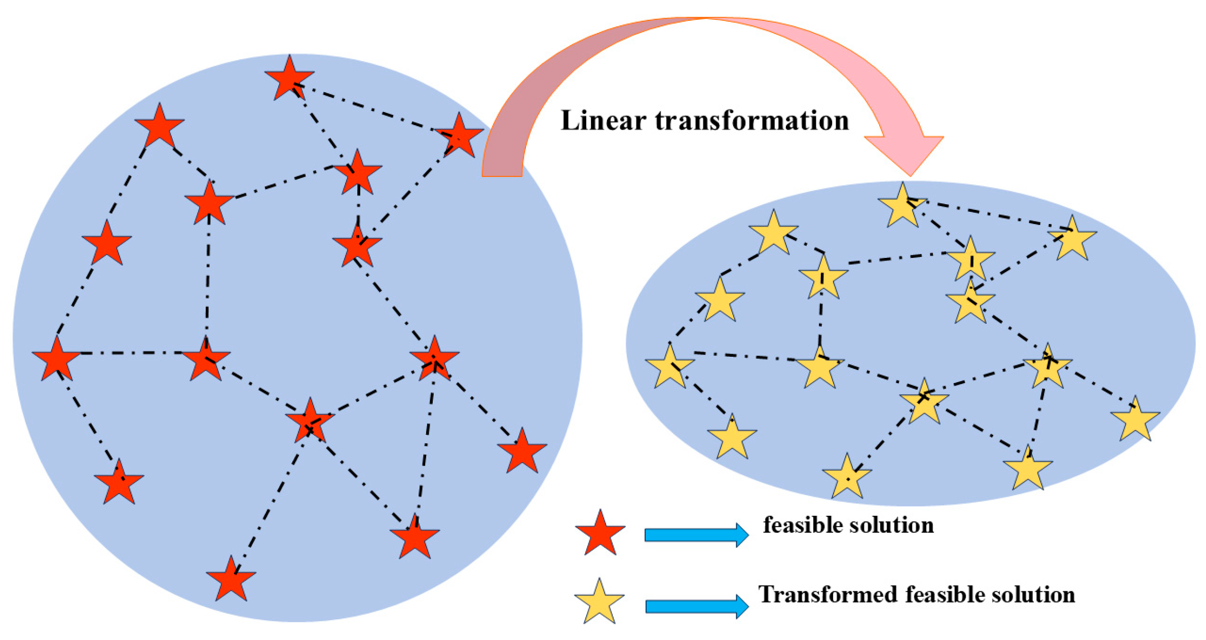
Analysis of the boomerang’s aerial motion indicates that its flight generates aerodynamic effects in the surrounding air. In the BAEO framework, when the feasible domain is two-dimensional, this aerodynamic influence zone is approximated as an ellipsoid, which defines the local search area around a solution. Consequently, BAEO introduces a novel strategy that enhances search capabilities for high-dimensional, complex objective functions while maintaining manageable spatio-temporal complexity. Based on heuristic mechanisms, this strategy enables discrete and uniform sampling of points on a three-dimensional ellipsoid. While illustrated using a three-dimensional example, the strategy extends naturally to higher-dimensional problems. To achieve uniform sampling on an ellipsoid, one may first perform uniform sampling on a sphere and then apply a linear transformation to map these points onto the ellipsoid, as illustrated in Figure 1.
Assuming the sphere’s center is located at the far point, and the random variables X, Y, and Z are independent and identically distributed with standard normal distributions, the probability density function for point X   Y   Z T in space is:
f x , y , x = 1 2 π 3 e x 2 + y 2 + z 2 2
From Equation (7) above, it can be seen that the probability density of a point depends solely on its distance from the origin, and is independent of the point’s spatial position and orientation. Random points uniformly distributed on a sphere can be generated by projecting points onto the sphere along the radial direction (i.e., the direction of the vector diameter). The specific formula is as follows:
x   y   z T = r X 2 + Y 2 + Z 2 X   Y   Z T
where r denotes the radius of the sphere. The probability density of a point on the sphere’s surface, which is the reciprocal of the surface area, is expressed as follows:
u = 1 4 π r 2
Next, a linear transformation maps points on the sphere onto the ellipsoid, where the ellipsoid’s three semi-axes are designated as a, b, and c. The following linear transformation maps random points on the sphere onto the ellipsoid; however, this transformation essentially stretches the sphere, resulting in non-uniform distribution of the mapped points on the ellipsoid.
p = ξ 2 b 4 c 4 + η 2 a 4 c 4 + ς 2 a 4 b 4 a 4 b 4 c 4
where p denotes the reception probability; a, b, and c represent the three semi-major axes of the ellipsoid; x, y, and z denote the coordinates of a point on the ellipsoidal surface. By combining linear transformations with the reception probability of random points, randomly and uniformly distributed points can be obtained on the ellipsoidal surface.
The aerodynamic effects generated by boomerang motion can be conceptualized as creating an ellipsoid centered at the origin, upon which a uniform random point search is performed. First, a set of points conforming to a normal distribution is generated with the current solution’s position as the center. These points are then mapped onto the high-dimensional ellipsoid based on their distance from the origin and the ellipsoid’s semi-major axis length, thereby achieving expansion in high-dimensional space. The specific expression is as follows:
p i , j = min h r i 2 · k = 1 dim X r i , j , k 2 t = 1 k 1 h r i , t 4 t = k + 1 dim h r i , t 4 t = 1 dim h r i , k 4
where p i , j represents the probability that the j-th position is accepted when multiple positions are generated on the ellipsoidal surface centered at the current position of the i-th boomerang. The number of positions generated in BAEO is 10. h r i , k denotes the semi-axis length in the k-th dimension of the ellipsoid generated centered at the current position of the i-th boomerang.
BAEO first randomly selects a portion of individuals from the population for aerodynamic search, setting this portion to one-fifth of the population size. Next, generate a set of points following a normal distribution around the selected i-th boomerang individual. Map these points to ellipsoidal space, calculate the acceptance probability for each location, and determine whether to select the current point based on this probability. Finally, identify the optimal solution among all selected points, compare it with the current solution, and update the optimal location.

2.2. Informer Model

The Informer model comprises an Encoder and a Decoder, following the sequence-to-sequence framework of the Transformer architecture [29]. The Encoder extracts features from input time series by capturing long-term dependencies through a multi-layer stacked self-attention mechanism combined with feedforward networks. The Decoder then generates predictions for future time steps based on the Encoder’s output, enabling the incremental construction of the target sequence.
To address the challenges of large parameter scales and high computational complexity encountered by traditional Transformers when modeling long sequences, Informer introduces targeted structural enhancements [30]. Specifically, it employs efficient attention mechanisms to reduce redundant computations and incorporates convolution and pooling operations within the Encoder to downsample feature sequences. Convolution captures local temporal features, while pooling compresses sequence length, thereby decreasing model parameters and computational overhead without compromising essential information. These improvements substantially enhance computational efficiency and predictive performance, rendering Informer particularly well-suited for long-term sequence forecasting tasks [31].

2.3. ARIMA Model

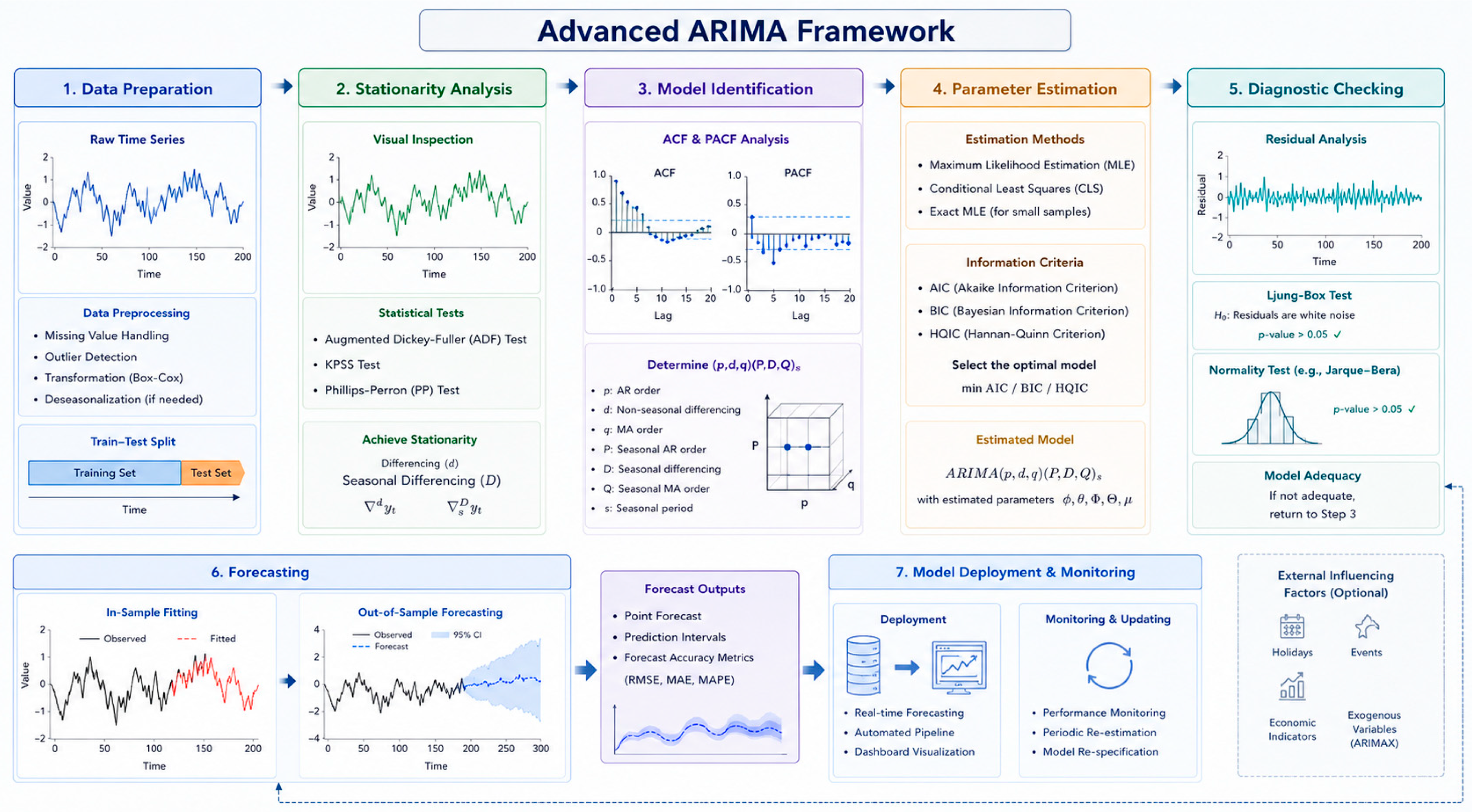
The ARIMA model is a model for analyzing random time series [32], which can capture the standard time structure in the time series through the probability analysis of the sequence itself. Specifically, the ARIMA model is divided into three parts, namely AR, I, and MA. Among them, AR represents the autoregressive model, I represents the differential model, and MA represents the moving average model. The ARIMA (p, d, q) model can establish a stationary sequence, where d is the order of difference, p is the autoregressive item, and q is the moving average item. The model structure is shown in Figure 2.
The mathematical expression of ARIMA model is as follows [33]:
1 i = 1 p α i L i ( 1 L ) d Y t = α 0 + 1 + i = 1 q β i L i ε t
where 1 i = 1 p α i L i is AR ( p ) , ( 1 L ) d Y t , ( 1 L ) d Y t is d Degree Differential, 1 + i = 1 q β i L i ε t is MA ( q ) . The ARIMA model is Y t ~ ARIMA ( p , d , q ) .

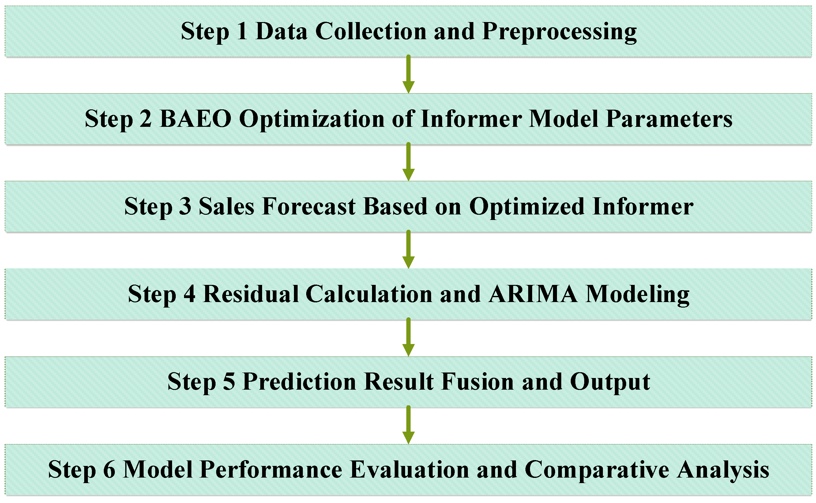
2.4. Construction of a Combined Predictive Model

To systematically characterize the temporal evolution of China’s new energy vehicle sales and enhance forecasting accuracy, this study constructs a hybrid forecasting model based on BAEO–Informer–ARIMA. The overall modeling process is shown in Figure 3 below. To avoid potential data leakage in the forecasting process, all data preprocessing procedures were conducted strictly according to chronological order. After the original dataset was divided into training and testing periods, feature engineering was performed only based on information available before each forecasting point. Specifically, lag variables and rolling statistical features were generated using historical observations without incorporating future samples. Moreover, normalization parameters were obtained exclusively from the training dataset, and the learned transformation was subsequently applied to the testing dataset. For provincial-level forecasting, historical records of each province were independently organized according to their actual timeline, and future forecasting was performed only after model training was completed. This procedure ensures that the evaluation results accurately represent the model’s real-world forecasting performance.
  • Step 1. Data Collection and Preprocessing
Collect monthly/annual sales data for new energy vehicles in China, integrating it with relevant statistical data on macroeconomics, policies, and industrial development. Perform missing value handling, outlier removal, and normalization on the raw data to construct a unified, continuous time series dataset, providing the foundational data for subsequent modeling.
  • Step 2. BAEO Optimization of Informer Model Parameters
Addressing the Informer model’s numerous hyperparameters and their sensitivity to predictive performance, BAEO is employed for global optimization of key Informer parameters. With prediction error minimization as the objective function, BAEO’s population initialization, fitness evaluation, position update, and iterative evolution processes yield the optimal parameter configuration for the Informer model. This enhances the model’s ability to capture nonlinear characteristics and long-term dependencies in new energy vehicle sales.
  • Step 3. Sales Forecasting Using Optimized Informer
Under the optimal parameter configuration obtained through BAEO optimization, the BAEO-Informer model is constructed to train and forecast the time series of China’s new energy vehicle sales. This model leverages Informer’s efficient attention mechanism to capture long-term trends and complex nonlinear variations within sales data, generating preliminary forecast results.
  • Step 4. Residual Calculation and ARIMA Modeling
Compare the BAEO-Informer predictions with actual sales data to compute the residual sequence. To address potential residual linear correlations and random fluctuations, an ARIMA model is applied to model and forecast the residual sequence, compensating for the limitations of deep learning models in linear modeling.
  • Step 5. Forecast Fusion and Output
The forecast results from BAEO-Informer and the ARIMA residual forecast are combined using Equation (13) to derive the final NEV sales forecast. This fusion approach fully leverages the strengths of both deep learning and statistical models, enabling a comprehensive characterization of sales variation patterns.
Y ^ t = Y ^ BAEO-Informer t + e ^ ARIMA t
  • Step 6. Model Performance Evaluation and Comparative Analysis
Quantitative assessment of the BAEO–Informer–ARIMA model’s predictive performance was conducted using evaluation metrics such as MAE, RMSE, and MAPE. Comparative analysis was performed against traditional ARIMA, single Informer, and other machine learning models to validate the proposed model’s effectiveness and superiority in forecasting China’s new energy vehicle sales. Different from conventional hybrid forecasting methods that simply combine multiple models, the proposed BAEO–Informer–ARIMA framework is developed based on a complementary modeling strategy. Specifically, BAEO is responsible for adaptive hyperparameter optimization of the Informer network, enabling automatic adjustment of model complexity according to forecasting characteristics. Informer focuses on extracting nonlinear temporal dependencies and long-range interactions from NEV sales-related variables, while ARIMA performs residual correction by capturing linear temporal information that remains unexplained by the deep learning component. Through the cooperation of these three modules, the proposed framework integrates adaptive optimization, nonlinear feature learning, and linear residual refinement, thereby improving the forecasting capability for complex NEV market dynamics.

3. Results Analysis

3.1. Data Acquisition and Preprocessing

This study aims to provide accurate forecasts for China’s new energy vehicle (NEV) sales. To this end, monthly data from January 2016 to December 2023 were collected from the China Statistical Yearbook [34], covering all 31 provincial-level administrative regions in China (excluding Hong Kong, Taiwan, and Macau). The analysis focused on key multidimensional variables to comprehensively capture the internal and external factors influencing NEV sales fluctuations. Infrastructure-related data were incorporated from the China Electric Vehicle Charging Infrastructure Promotion Alliance, including the number of public charging piles and the monthly construction scale of battery-swapping stations [35], reflecting the role of infrastructure development in supporting NEV adoption. Travel-demand indicators from the transportation sector, including passenger volume and passenger turnover [36], were selected to capture macro-level changes in mobility and their impact on the NEV market. To account for market stock effects, data on NEV ownership were also included. Furthermore, carbon emission indicators for the transportation sector [37] were integrated to represent the potential influence of low-carbon transition pressures and environmental constraints on consumer decisions under China’s “dual-carbon” policy framework. Collectively, these six features provide a systematic and comprehensive multidimensional basis for the forecasting model, spanning infrastructure, transportation demand, market scale, and environmental constraints, thereby enhancing the accuracy and reliability of NEV sales projections.
To eliminate the impact of different feature dimensions on model training, the collected multi-source data (including sales volume, vehicle ownership, charging station count, etc.) is first normalized. The Min-Max normalization method is employed to map the data to the [0, 1] range:
x = x x m i n x m a x x m i n
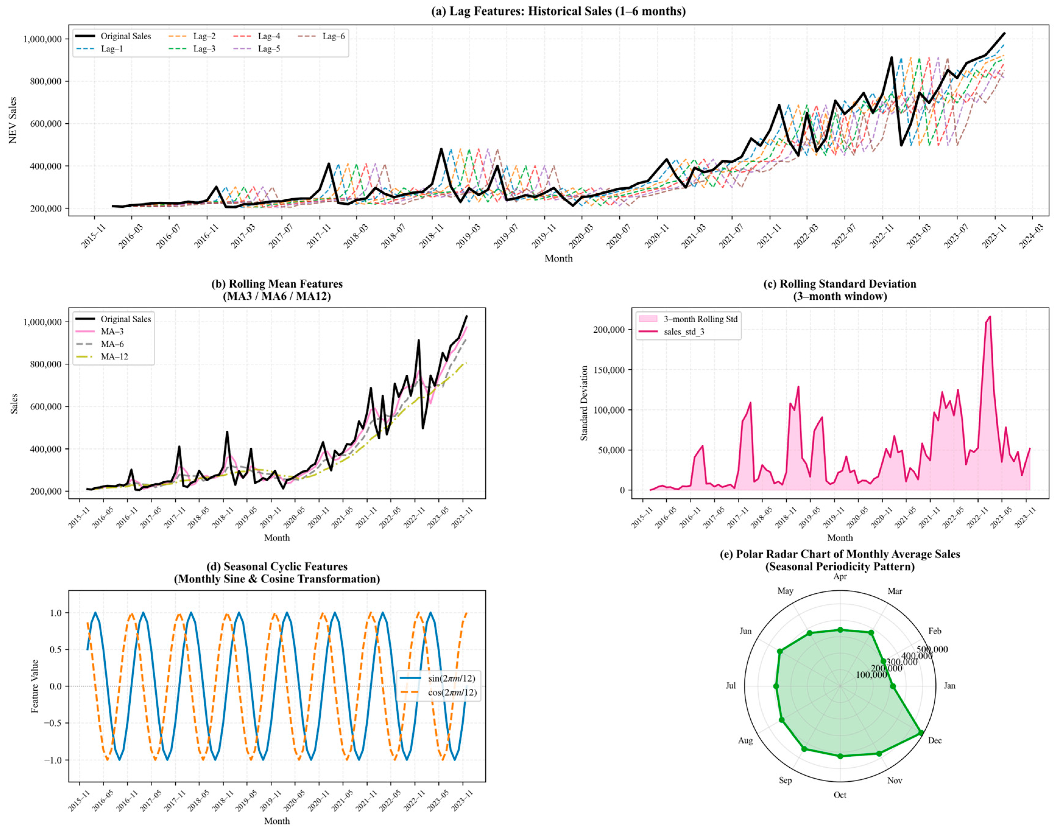
During the feature construction phase, to more fully capture the historical dependencies and dynamic evolution characteristics within the time series of new energy vehicle sales, this study incorporates lag features [38] and rolling statistical features [39]. Specifically, sales data from the preceding 1–6 months is included as lagged variables in the model inputs to reflect the inertia and continuity of sales over time. Simultaneously, we computed moving averages and moving standard deviations over 3-, 6-, and 12-month windows to capture short-term fluctuations and medium-to-long-term trends. This feature construction enables the model to learn the temporal structure of sales sequences more comprehensively, thereby enhancing prediction performance and stability. Additionally, monthly sine and cosine transform features ( sin ( 2 π m / 12 ) , cos ( 2 π m / 12 ) ) were incorporated to model seasonal patterns in sales data, with results shown in Figure 4.
As shown in Figure 4a, the NEV sales series exhibits pronounced temporal dependency. The overall trends of the 1–6-month lagged terms closely follow the original sales curve, with only minor phase shifts, indicating strong short-term inertia and continuity in sales. During the rapid growth phase after 2021, the lagged curves continue to track the overall trend effectively, demonstrating that historical sales data possess substantial predictive value for future sales. Consequently, incorporating multi-order lag features allows the model to capture the autocorrelation structure of sales, enhancing time series forecasting accuracy. Figure 4b presents moving average (MA) characteristics over different time windows. Compared with the raw sales curve, MA3 is more sensitive to short-term fluctuations, reflecting cyclical volatility, whereas MA6 and MA12 provide smoother representations that capture medium- to long-term growth trajectories. Notably, during periods of rapid sales expansion, the MA12 curve maintains a stable upward trend, assisting the model in identifying long-term growth patterns while reducing the influence of anomalous fluctuations on forecast outcomes. Figure 4c illustrates standard deviation variations using a 3-month sliding window, highlighting distinct differences in sales volatility across periods. Overall volatility was relatively low from 2016 to 2019 but increased sharply after 2020, with pronounced peaks corresponding to policy stimulus events or concentrated market demand releases. This indicates that the rapid expansion of the NEV market is accompanied by substantial instability. Including the sliding standard deviation feature enables the model to dynamically detect high-volatility intervals, thereby improving forecast robustness. Figure 4d depicts seasonal cycle characteristics obtained through sine and cosine transformations of monthly data. Periodic coding effectively mitigates the discontinuity inherent in integer month variables (“January–December”), ensuring smooth transitions between December and January in the feature space. Both sine and cosine curves exhibit regular periodic fluctuations, capturing the annual cycle structure and providing continuous seasonal information for the model. Figure 4e shows the seasonal distribution of monthly average sales in polar coordinates. NEV sales clearly peak at the end of the year, particularly in November and December, while remaining relatively low at the beginning of the year, forming an annual cycle pattern of “low at the start, high at the end.” This pattern may be influenced by factors such as annual subsidy policies, automaker promotions, and concentrated year-end purchasing demand. The polar coordinate representation intuitively reveals cyclical sales fluctuations, further validating the inclusion of seasonal feature variables in the model.

3.2. Research on Sales Distribution Trends of New Energy Vehicles

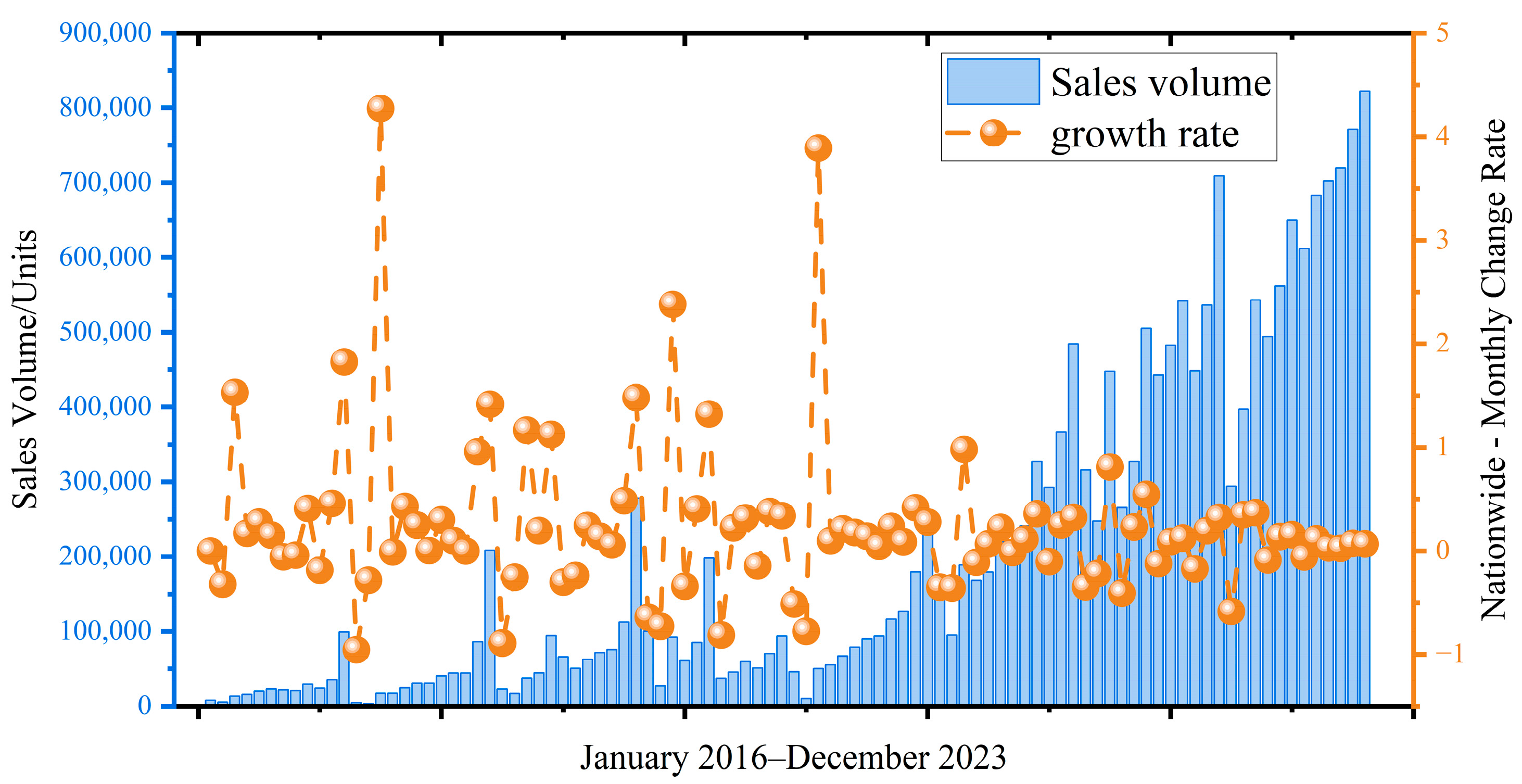
Based on the monthly sales volumes (vehicles/month) and month-over-month growth rates of China’s new energy vehicles (NEVs) from January 2016 to December 2023 (Figure 5), the phased evolution and overall development trends of the NEV market can be systematically analyzed. Overall, NEV sales exhibit a pronounced long-term upward trajectory, accompanied by significant volatility and structural shifts across different phases, reflecting the combined influence of policy environments, market maturity, and external shocks.
During the initial phase from 2016 to 2018, the market scale remained small, with low monthly sales baselines, resulting in substantial fluctuations in growth rates and pronounced positive and negative swings in certain months. This phase was primarily constrained by factors such as adjustments to subsidy policies, limited market acceptance, and insufficient infrastructure, making sales highly sensitive to short-term policy changes and market expectations. From late 2018 to 2019, sales rebounded overall but remained volatile, indicating the industry’s transition from policy-driven to market-driven growth.
Entering 2020, NEV sales experienced a structural leap, with monthly volumes expanding substantially. Although temporary declines occurred in certain months due to macroeconomic conditions and the COVID-19 pandemic, the overall growth trend remained robust. In particular, between 2021 and 2023, sales continued to rise, with monthly growth rates gradually converging to a more stable range, signaling gradual market maturation and increased consumer acceptance of NEVs. Peaks in monthly growth were often associated with policy incentives, concentrated model launches, or year-end delivery surges, whereas months of negative growth generally reflected temporary adjustments that did not alter the long-term upward trajectory.
Collectively, the temporal evolution of NEV sales follows a pattern of “low base with high volatility → scale expansion → steady growth.” Monthly growth rates have shifted from early-stage volatility to relative stability in later phases, indicating that China’s NEV industry is transitioning from policy-dependent to market-driven expansion. These characteristics provide crucial guidance for sales forecasting: models must capture the long-term upward trend while accounting for short-term fluctuations and cyclical effects on sales volumes.
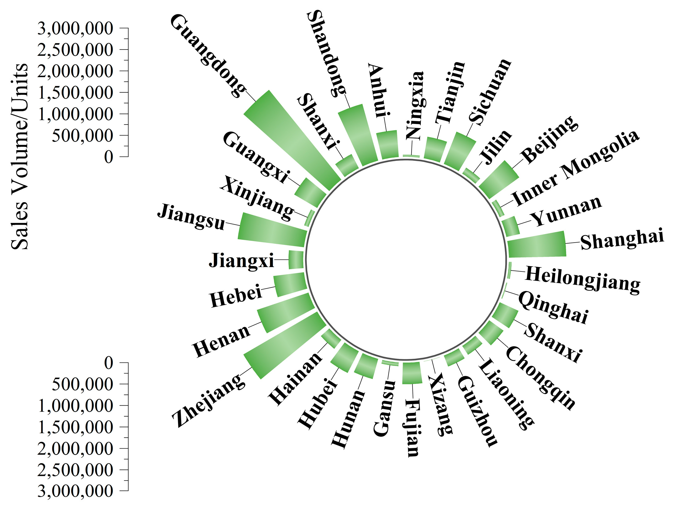
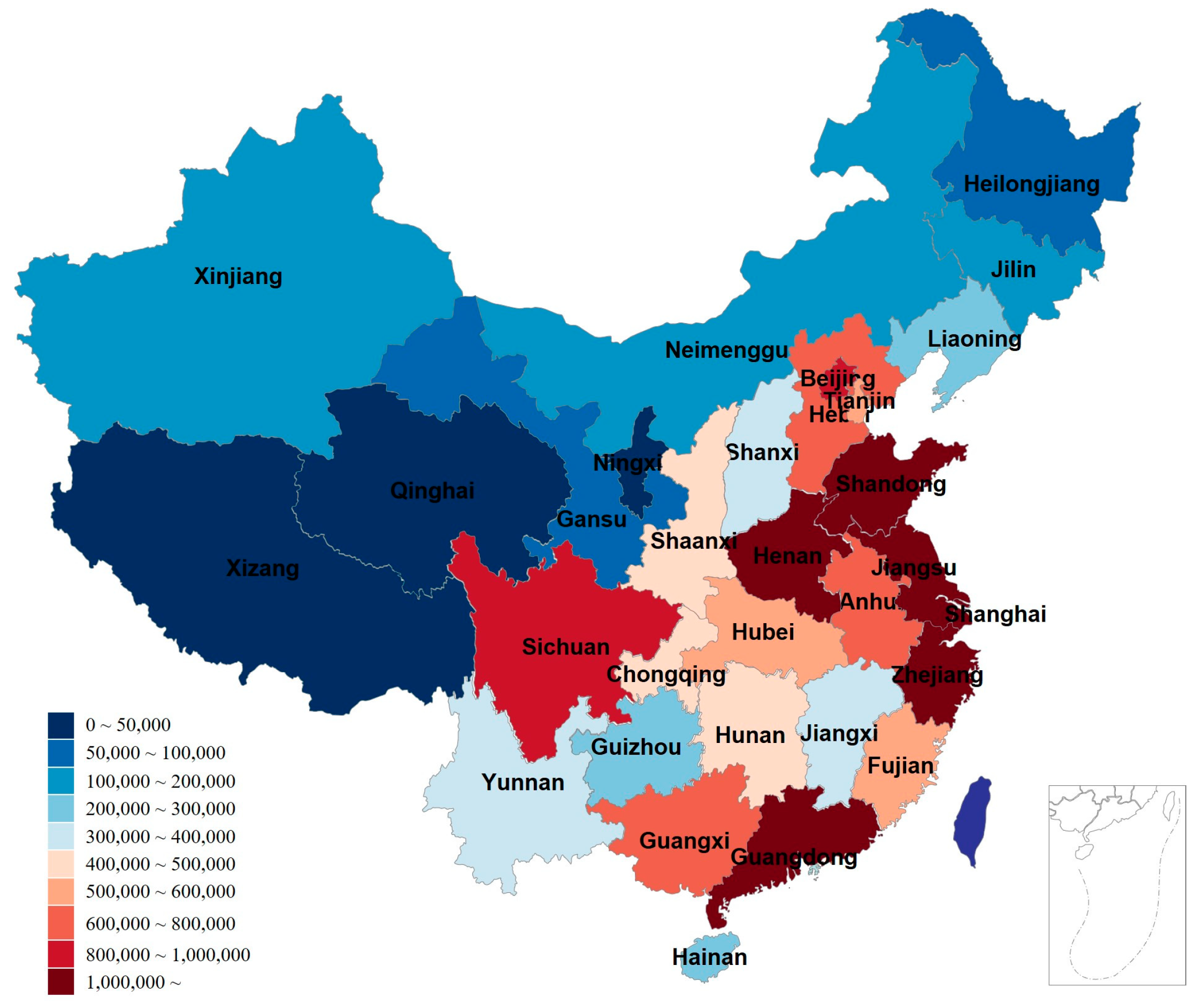
Based on cumulative NEV sales data across Chinese provinces from 2016 to 2023 (Figure 6 and Figure 7), the development characteristics of China’s NEV market can be systematically analyzed from two perspectives: regional-scale differences and spatial distribution patterns. Overall, provincial NEV sales exhibit pronounced spatial heterogeneity, with clear regional clustering effects closely associated with economic development, industrial base, population size, and policy support.
In terms of sales scale, Guangdong, Jiangsu, Zhejiang, Shandong, Shanghai, and Henan reported cumulative NEV sales well above the national average. Guangdong leads the nation with a dominant margin, reflecting its large automotive consumption market, well-developed NEV industrial chain, and sustained local policy support. Similarly, the Yangtze River Delta provinces—Jiangsu, Zhejiang, and Shanghai—demonstrate a notable first-mover advantage and scale effect in NEV adoption, highlighting the benefits of economic development in facilitating technology diffusion. In contrast, western provinces such as Tibet, Qinghai, Ningxia, and Xinjiang exhibit substantially lower sales, indicating that NEV promotion in low-population-density areas with limited infrastructure remains constrained. Regarding spatial distribution, the regional heatmap in Figure 7 further illustrates the clustering pattern of NEV sales. Overall, the distribution follows an “east strong–west weak, south high–north low” pattern, with high-value clusters concentrated in the economically active eastern coastal and central provinces, while the northwest and parts of the northeast form low-value areas. These spatial disparities are closely linked not only to regional economic development but also to the distribution of charging and battery-swapping infrastructure, resident mobility patterns, and local government incentive policies for NEVs. Notably, central provinces such as Henan, Anhui, and Hubei exhibit mid-to-upper-level sales, indicating a gradual diffusion of the NEV market from coastal to inland regions.

3.3. Factors Affecting New Energy Vehicle Sales Volume

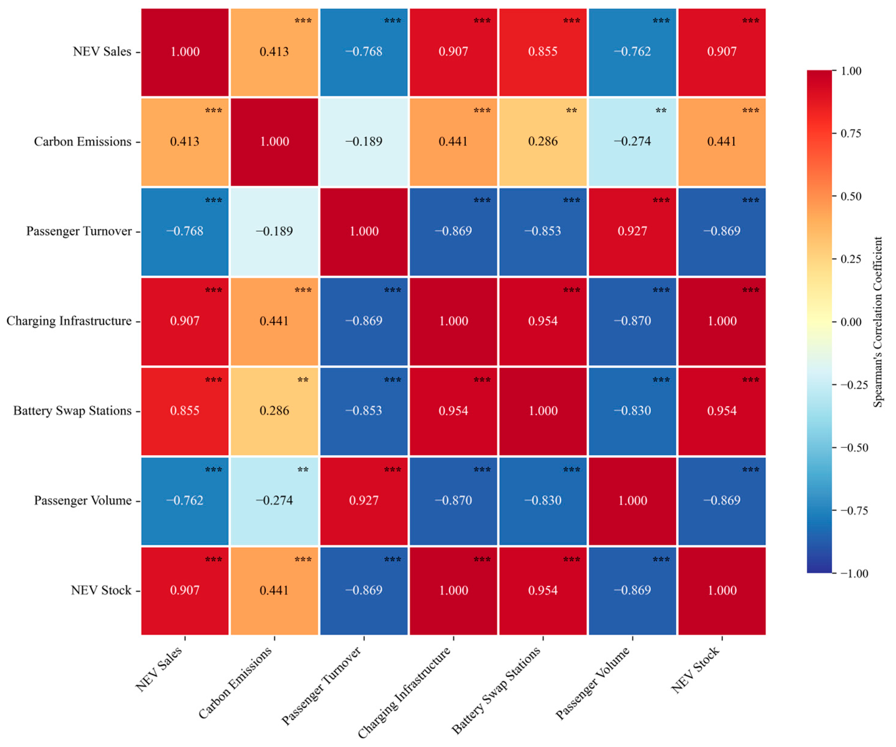
To systematically analyze the correlation between new energy vehicle sales and various influencing factors, this study employs Spearman’s rank correlation coefficient to quantitatively assess the relationship between China’s new energy vehicle sales and the aforementioned six characteristic variables. The results are presented as a correlation heatmap in Figure 8. Spearman’s correlation coefficient is a nonparametric statistical method based on ranks, independent of the specific distribution of variables. It effectively captures monotonic relationships between variables and can be calculated using Equation (15). Consequently, this method demonstrates greater robustness than Pearson’s correlation coefficient in analyzing time series data like new energy vehicle sales, which exhibit significant periodicity and volatility.
r s = 1 6 i = 1 n d i 2 [ n ( n 2 1 ) ]
where di is the rank difference between the two sets of data Xi and Yi. rs ranges between −1 and 1.
As shown in Figure 8, Spearman’s correlation analysis reveals that new energy vehicle (NEV) sales exhibit extremely significant correlations at the p < 0.001 level with all selected variables. Specifically, NEV sales demonstrate extremely strong positive correlations with charging infrastructure ( r = 0.907 ), NEV stock ( r = 0.907 ), and battery swapping stations ( r = 0.855 ); a significant negative correlation with passenger transport turnover and passenger volume ( r = 0.76 ); and a moderate positive correlation with carbon emissions ( r = 0.413 ). This indicates that infrastructure deployment and market scale are core drivers of sales growth, while also revealing the complex co-evolutionary relationship between NEV promotion, traditional passenger transport modes, and carbon emission metrics during the low-carbon transportation transition.

3.4. Model Parameter Configuration and Evaluation Metric Determination

3.4.1. Hyperparameter Optimization of the BAEO-Based Informer Model

The predictive performance of the Informer model is highly dependent on hyperparameter settings. Improper parameter selection may cause the model to get stuck in local optima or suffer from overfitting. This study employs the BAEO algorithm to adaptively optimize five key hyperparameters of Informer: learning rate, hidden layer size, sequence length, batch size, and dropout rate.
The optimization process is as follows:
(1)
Population Initialization: Initialize the BAEO population, where each “boomerang” individual represents a potential hyperparameter combination vector X i = [ l r , h i d d e n , s e q _ l e n , b a t c h , d r o p o u t ] .
(2)
Fitness Evaluation: Substitute each set of hyperparameters into the Informer model, then train and predict on the validation set, using mean squared error (MSE) as the fitness function.
f i t n e s s ( X i ) = M S E v a l i d a t i o n = 1 N t = 1 N ( y t y ^ t ) 2
where N represents the number of samples in the validation set; y t denotes the true value; and y ^ t indicates the predicted value.
(3)
Position Update: Continuously update the position of each individual based on the BAEO’s spiral mechanism and aerodynamic elliptical search strategy.
In the t-th iteration, the position update for each individual follows the following strategy:
X i t + 1 = 1 3 ( X 1 + X 2 + X 3 )
where X 1 = α p o s A 1 | C 1 α p o s X i t | ; X 2 = β p o s A 2 | C 2 β p o s X i t | ; X 3 = δ p o s A 3 | C 3 δ p o s X i t | .
The algorithm parameter a decreases linearly with iteration: a = 2 t 2 T m a x , where T m a x = 100 represents the maximum iteration count.
(4)
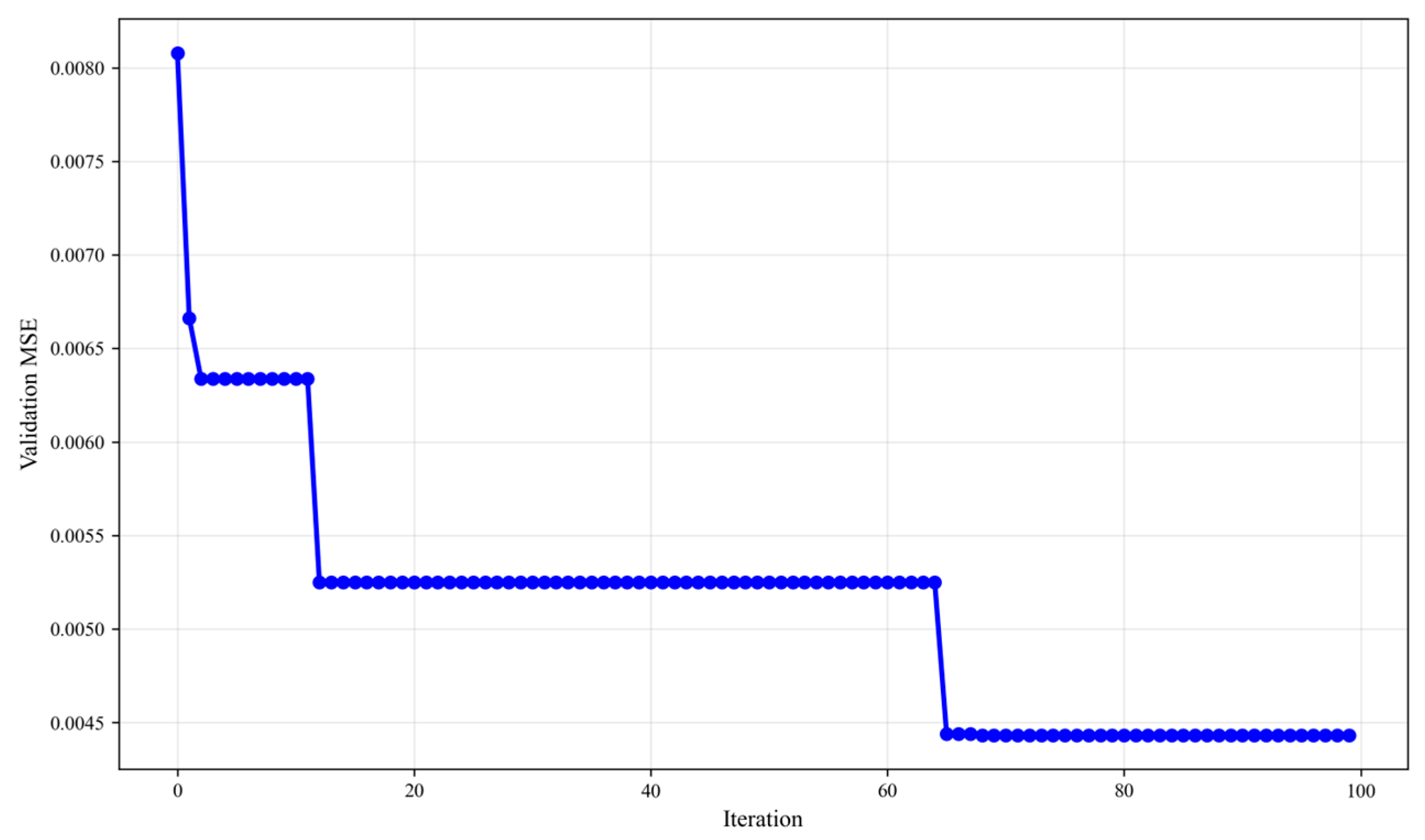
Output optimal solution: After 100 iterations, the set of hyperparameters with the minimum fitness (i.e., lowest validation set error) is output for constructing the final Informer prediction model. The optimization results are shown in Table 1 and Figure 9.
As shown in Figure 9, the validation set MSE exhibits an overall stepwise decline with increasing iterations. The error remains high initially but decreases rapidly within the first 10 iterations, indicating the algorithm’s ability to swiftly locate the optimal solution region. Subsequently, a noticeable plateau emerges around the 15th iteration, signifying entry into a locally stable search phase. After the 60th iteration, the error again decreased significantly and stabilized, ultimately settling near 0.004432. The overall convergence process was smooth with no noticeable oscillations, demonstrating that the BAEO algorithm possesses strong global search capabilities and convergence stability, achieving significant optimization results.

3.4.2. Determination of Model Evaluation Metrics

R2 (Coefficient of Determination) is a key statistical indicator for measuring the goodness-of-fit of a regression model to data, reflecting the model’s ability to explain sample variance [40]. Its value typically ranges between [0, 1], with values closer to 1 indicating better model fit to the actual data. Negative values suggest poor model fit, which is potentially worse than simply using the sample mean for prediction. The definition and calculation formula for R2 are as follows in Equation (18):
R 2 = 1 i = 1 n y i y ^ i 2 i = 1 n y i y ¯ 2
where y i represents the true value of the i-th sample; y ^ i represents the predicted value of the i-th sample; y ¯ represents the mean of the true values.
Mean Absolute Error (MAE) measures the average deviation between a model’s predicted values and actual values, serving as a common metric for evaluating the predictive accuracy of regression models [41]. This metric reflects overall prediction bias by calculating the average of the absolute values of prediction errors, assigning equal weight to all errors. It provides an intuitive representation of the average deviation of prediction results. Its formula is:
MAE = 1 n i = 1 n y i y ^ i
Mean Squared Error (MSE) is a crucial metric for evaluating the predictive performance of regression models, calculated as the average of the squared differences between predicted and actual values [42]. Unlike MAE, MSE assigns greater weight to larger prediction errors, thereby more sensitively reflecting the impact of extreme deviations on model performance. Its formula is:
MSE = 1 n i = 1 n y i y ^ i 2
Root Mean Squared Error (RMSE) is a commonly used metric for evaluating the predictive accuracy of regression models. It is defined as the square root of the Mean Squared Error (MSE) [43]. By taking the square root, RMSE restores the error’s dimensionality to match that of the original data, making the error values more intuitive and easier to interpret. It also exhibits high sensitivity to larger deviations. Its formula is:
RMSE = 1 n i = 1 n y i y ^ i 2
The symbols in Equations (19)–(21) have the same meanings as above.

3.5. Analysis of Model Prediction Results

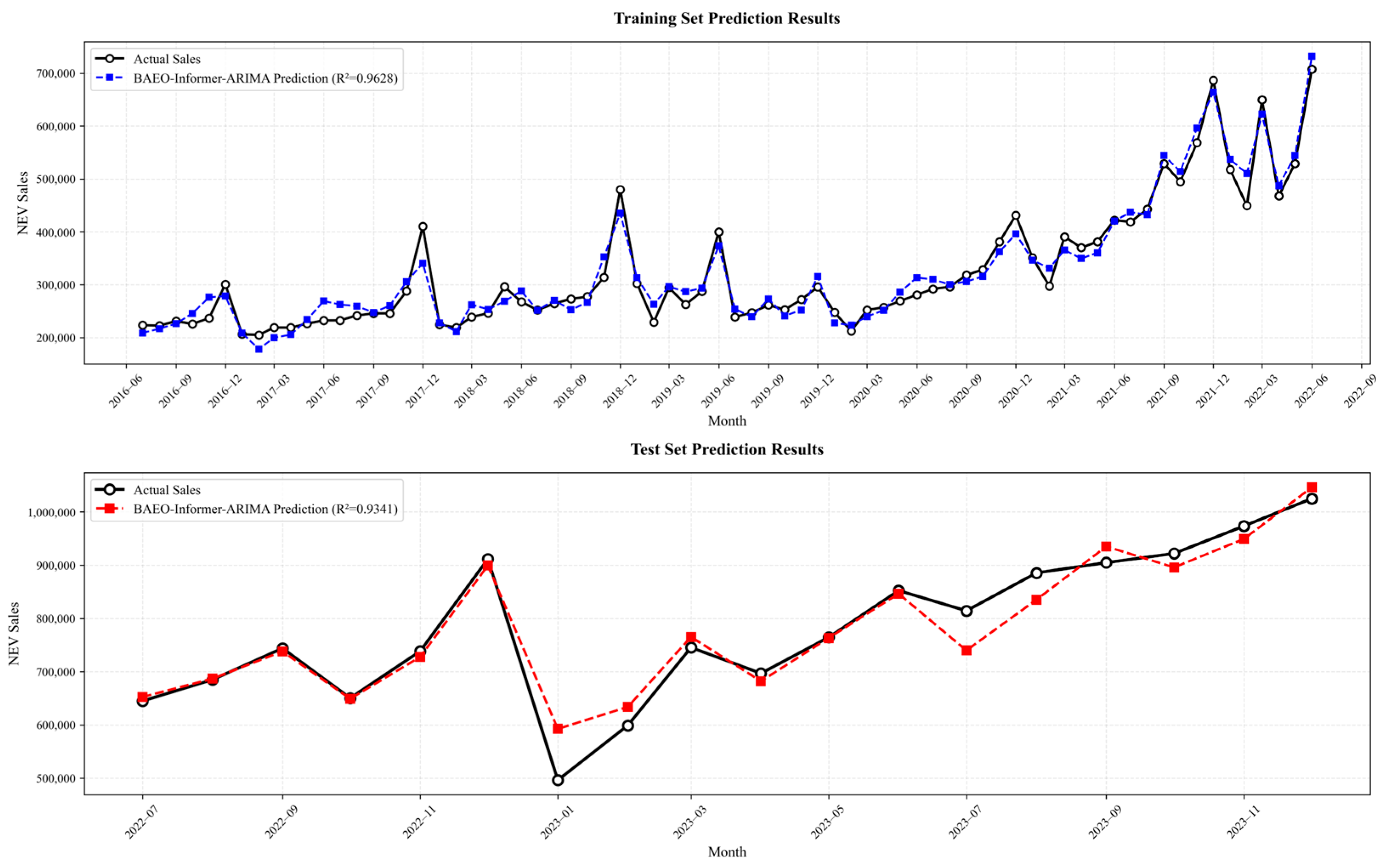
This study employs a BAEO-optimized Informer–ARIMA hybrid forecasting model to predict new energy vehicle (NEV) sales, with the dataset divided into training and testing sets according to an 80:20 chronological ratio. Figure 10 presents the prediction performance of the proposed model on both training and testing datasets.
As shown in Figure 10 (top), the proposed model achieves excellent fitting performance on the training dataset. The predicted curve (blue dashed line) closely follows the actual sales curve (black solid line), achieving an R2 value of 0.9798. This indicates that the model effectively captures the underlying temporal characteristics of NEV sales, including long-term growth trends and periodic fluctuations. Specifically, the model accurately represents the rapid expansion trend of China’s NEV market from 2016 to 2023, particularly during the accelerated growth period after 2020. During this stage, monthly NEV sales increased significantly, reflecting the combined effects of technological progress, policy incentives, charging infrastructure development, and increasing consumer acceptance. Meanwhile, the model successfully captures seasonal variation characteristics, including the sales decline associated with the Spring Festival period and the year-end sales increase caused by concentrated purchasing and registration activities. For example, the model provides relatively accurate predictions for the sales decline in February 2021 and the peak sales period in December 2021, demonstrating its ability to characterize both trend evolution and short-term periodic fluctuations.
According to the chronological division strategy, the monthly NEV sales data from January 2016 to December 2023 contain 96 observations, of which the first 77 months were used for model training and the remaining 19 months were used for testing. For visualization purposes, Figure 10 (bottom) displays the prediction results for the representative testing period from January to November 2023, while the complete testing dataset was retained for quantitative evaluation. The results show that the predicted values generally agree well with the actual observations, indicating that the proposed model maintains strong generalization capability when applied to unseen data.
Although the proposed model demonstrates high prediction accuracy, several observations still show relatively larger deviations between the predicted and actual values. These discrepancies mainly occur during periods characterized by rapid market changes or abnormal fluctuations. One possible reason is that NEV sales are influenced not only by historical sales patterns but also by external factors, such as government subsidy policies, purchase incentives, supply-chain conditions, battery technology development, and consumer behavior changes. Such factors may introduce sudden variations that are difficult to fully capture using historical time-series information alone. In addition, China’s NEV market has experienced a transition from early-stage expansion to large-scale commercialization, resulting in nonlinear growth characteristics and increased forecasting complexity. During periods with sharp sales increases, the actual values may exceed model predictions because of unexpected market stimulation, such as policy adjustments, promotional activities, or concentrated consumer demand. Conversely, temporary declines may be related to seasonal effects, holiday impacts, or short-term market saturation. Although the BAEO algorithm improves parameter optimization, the Informer model enhances long-term dependency extraction, and ARIMA provides residual correction, unavoidable forecasting errors may still exist due to the inherent uncertainty of the rapidly evolving NEV market.
Overall, the BAEO–Informer–ARIMA hybrid model demonstrates strong capability in capturing long-term trends, seasonal patterns, and nonlinear characteristics of NEV sales. The analysis of prediction deviations further confirms that the remaining errors are mainly associated with external market uncertainties rather than model instability. These results verify the effectiveness and practical applicability of the proposed framework for NEV sales forecasting and provide valuable quantitative support for industrial planning, charging infrastructure deployment, and low-carbon policy formulation.
Table 2 lists four key evaluation metrics for the model on the training and test datasets: Root Mean Square Error (RMSE), Mean Absolute Error (MAE), Coefficient of Determination (R2), and Mean Absolute Percentage Error (MAPE). The MAPE on the training set is 3.48%, and on the test set it is 3.39%. Both mean absolute percentage errors are below 5%, meeting the criteria for high-precision prediction.
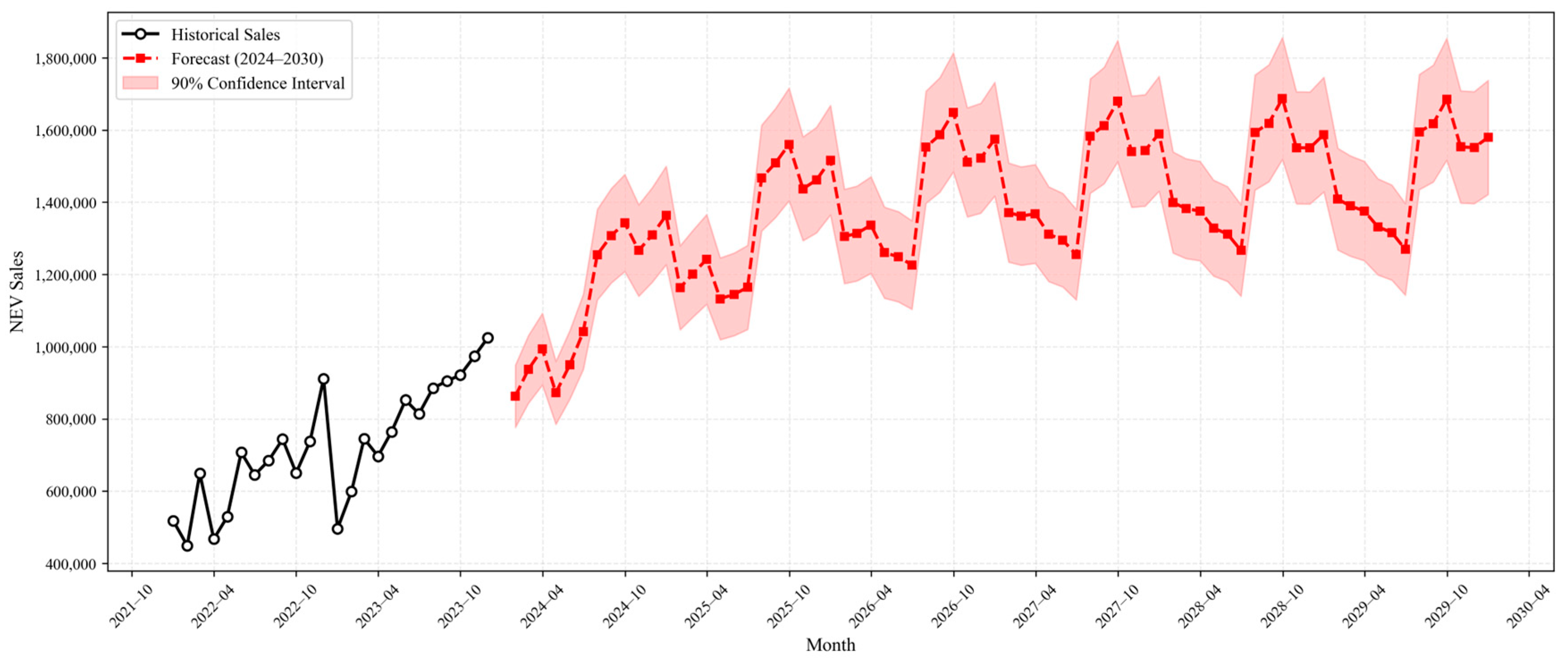
Based on the trained BAEO–Informer–ARIMA composite model, this study conducts medium- to long-term forecasts of monthly China’s new energy vehicle (NEV) sales volume from 2024 to 2030 (Figure 11). The results suggest that the overall market will sustain its growth momentum, although the pace is expected to decelerate periodically. As NEV market penetration continues to increase, the potential for incremental demand gradually diminishes. Accordingly, the sales growth trajectory shifts from early-stage exponential expansion toward a more linear pattern, with possible short-term fluctuations or structural adjustments in specific phases. This evolution is consistent with classical technology diffusion and industrial life-cycle theory, whereby rapid expansion is followed by entry into a relatively stable development stage.
The forecasts further indicate that seasonal fluctuations will persist, with annual sales exhibiting a regular pattern of alternating peaks and troughs. Monthly sales are projected to remain relatively low from January to February, influenced by the Spring Festival holiday, fewer working days, and deferred purchasing decisions. From March to August, the market is expected to operate steadily with limited volatility, whereas September to December is likely to constitute the annual peak period, driven by promotional campaigns, year-end sales targets, and concentrated new model launches—reflecting a pronounced “year-end surge” effect. These results demonstrate that the model not only captures long-term growth trends but also effectively extrapolates historical seasonal dynamics.
Although the BAEO–Informer–ARIMA pipeline produces deterministic point forecasts, forecast uncertainty can be estimated from its historical out-of-sample errors. In this study, one-step-ahead residuals from the rolling validation period were used to estimate the forecast-error standard deviation. For a forecast horizon h, the corresponding standard error was adjusted to reflect the accumulation of uncertainty with the forecast horizon, and the 90% confidence interval was calculated as the point forecast plus or minus 1.645 times the horizon-specific standard error. The 90% confidence level was selected because it provides a practical balance between statistical coverage and interval width: an excessively high confidence level produces intervals that are too wide for operational planning, whereas a lower confidence level may understate market uncertainty. The 5th and 95th percentile limits therefore provide an interpretable range for medium- and long-term policy and capacity-planning decisions. For example, the projected monthly sales volume for June 2027 is approximately 115,000 vehicles/month, with a 90% confidence interval of approximately 92,000–138,000 units. The interval gradually widens at longer horizons because forecasting errors and external market uncertainty accumulate over time.
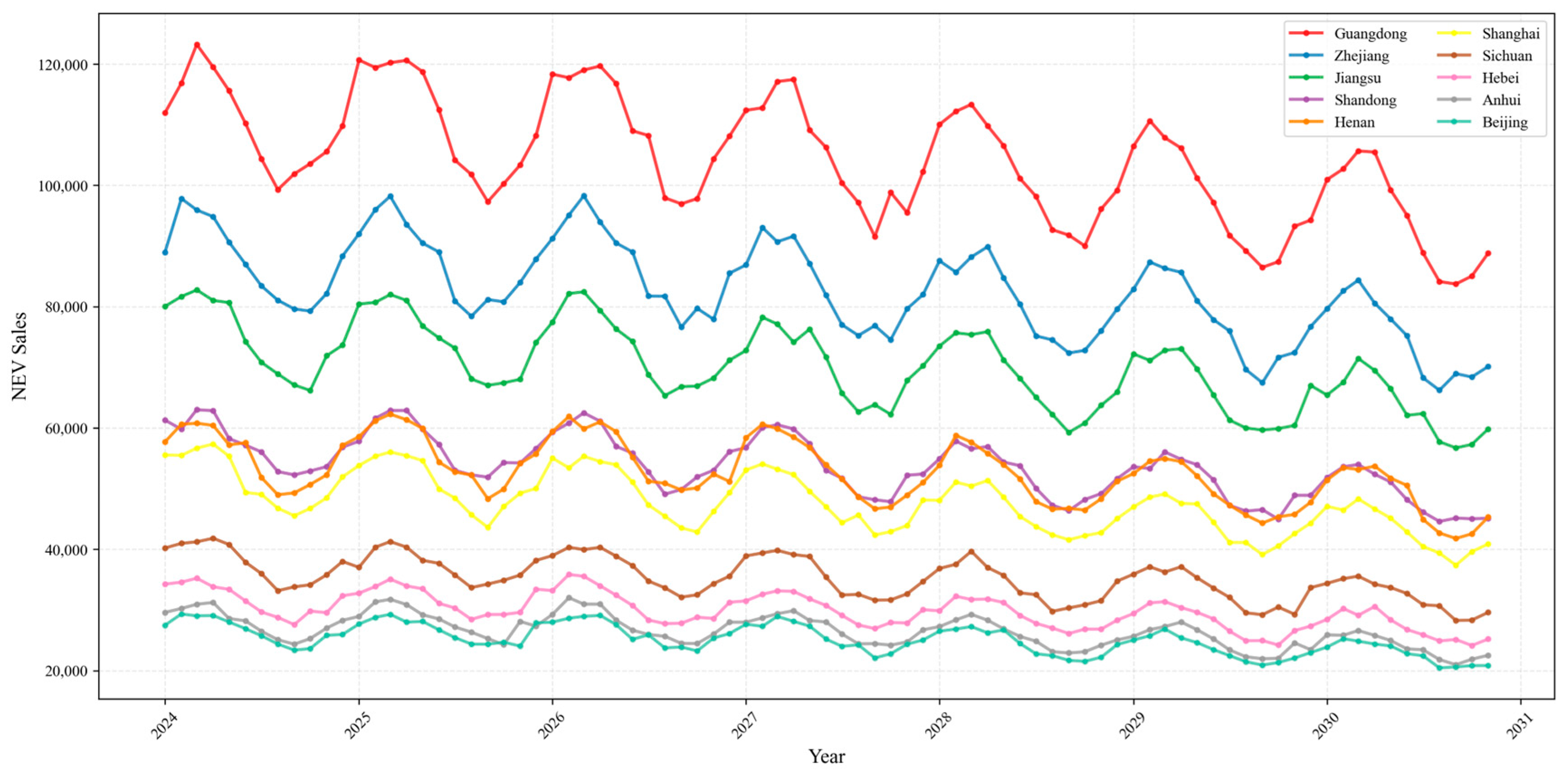
Figure 12 presents the forecast results for the top 10 provinces in new energy vehicle sales from 2024 to 2030 based on the BAEO–Informer–ARIMA combined model. It should be clarified that these provincial-level forecasts were generated using the same trained forecasting framework, rather than establishing separate models for each province. Specifically, the proposed model was trained using the integrated multi-source dataset containing provincial-level NEV sales and related influencing factors. After model training, historical data from each individual province were input into the same optimized model to obtain province-specific future sales forecasts. Therefore, the differences among provincial prediction results mainly originate from variations in historical sales patterns, infrastructure development, market penetration, and other regional characteristics, rather than from different model structures or parameter settings. This strategy ensures methodological consistency and enables a fair comparison of future NEV development trends across different provinces. It illustrates their sales performance and the pronounced seasonal fluctuation patterns. Future growth potential for new energy vehicles is narrowing, with variations in market bases and decline rates across provinces. This reflects deepening market penetration rates of new energy vehicles in different regions and validates the effectiveness of this forecasting framework in capturing regionally differentiated growth patterns.

3.6. Comparison of Prediction Results Across Different Models

Based on the aforementioned dataset partitioning scheme, this study systematically validated the predictive performance of the proposed BAEO–Informer–ARIMA model for forecasting China’s new energy vehicle sales. Specifically, the model’s predictions were compared against those of Informer, ARIMA, Informer-ARIMA, and BAEO-Informer. The comprehensive performance evaluation results are summarized in Table 3. To comprehensively evaluate each model’s performance in terms of forecasting accuracy and stability, four quantitative metrics were selected: the coefficient of determination R2, mean absolute error (MAE), mean squared error (MSE), and root mean squared error (RMSE).
By comparing the evaluation metrics in Table 3, it is evident that the proposed BAEO–Informer–ARIMA model demonstrates significant superiority and robustness in forecasting new energy vehicle sales. The model achieves optimal R2 values on both the training and test datasets, while simultaneously attaining the lowest values for error metrics such as MSE, MAE, and RMSE. This performance markedly outperforms the Informer, ARIMA, and their variant models. This indicates that incorporating the BAEO optimization strategy not only effectively enhances the feature extraction capability of the Informer model but also, through complementary synergies with ARIMA, further strengthens the model’s fitting accuracy for complex fluctuations and trends in sales sequences. This demonstrates that the combined forecasting framework possesses superior predictive performance and generalization potential when handling such time series forecasting tasks.
To provide a more rigorous baseline comparison, SARIMA, Prophet, XGBoost, LSTM, GRU, Transformer, and Informer were implemented under the same forecasting protocol as the proposed model. All models used an identical chronological 80:20 split, comprising 77 training months and 19 test months, and were evaluated using the same test window. The same lagged variables, rolling statistical features, seasonal encodings, and training-set-based Min–Max normalization were used whenever applicable. Hyperparameters were selected using only the training and validation periods, and no future observations were introduced during feature construction, normalization, or model fitting. The resulting test-set performance is summarized in Table 4.
As shown in Table 4, the BAEO–Informer–ARIMA model achieved the highest test-set R2 and the lowest MAE, RMSE, and MAPE among all evaluated methods. The statistical baselines, SARIMA and Prophet, were less effective in representing the nonlinear and rapidly changing characteristics of the NEV market. XGBoost improved nonlinear feature mapping but did not explicitly capture long-range sequential dependence. LSTM and GRU provided stronger temporal representations, while Transformer further improved long-range modeling. Nevertheless, the proposed framework retained the best overall performance because BAEO improved hyperparameter selection, Informer captured long-term nonlinear dependencies, and ARIMA corrected the remaining linear residual structure.

3.7. Feature Contribution Analysis

Ensemble models demonstrate exceptional fitting capabilities in time series forecasting, yet their complex network structures create a “black box” problem, making it difficult to intuitively interpret how individual input features influence final predictions. This study introduces SHAP (SHapley Additive exPlanations) to conduct interpretability analysis on the predictive model, quantitatively assessing the relative importance of each factor in driving new energy vehicle sales growth and revealing the positive or negative effects of different features on sales volume.
The SHAP method is based on the Shapley Value from cooperative game theory. Its core principle involves assigning a unique attribution value to each input feature by evaluating its marginal contribution across all possible feature combinations [44]. Compared to traditional feature importance evaluation methods, SHAP exhibits both local accuracy and global consistency. It not only outputs a global ranking of feature contributions but also explains the push–pull effects of features on individual prediction samples. For a given prediction model f and input sample x, the SHAP value ϕ i for feature i is calculated as shown in Equation (22):
ϕ i ( f , x ) = S N { i } | S | ! ( | N | | S | 1 ) ! | N | ! [ f x ( S { i } ) f x ( S ) ]
where N denotes the set of all input features in the model; S represents any subset of features excluding feature f x ( S ) ; |N| and |S| denote the number of features in set N and subset S, respectively; f x ( S ) indicates the model’s expected output when using only the features in subset S; f x ( S { i } ) f x ( S ) quantifies the marginal prediction change brought about by introducing feature i .
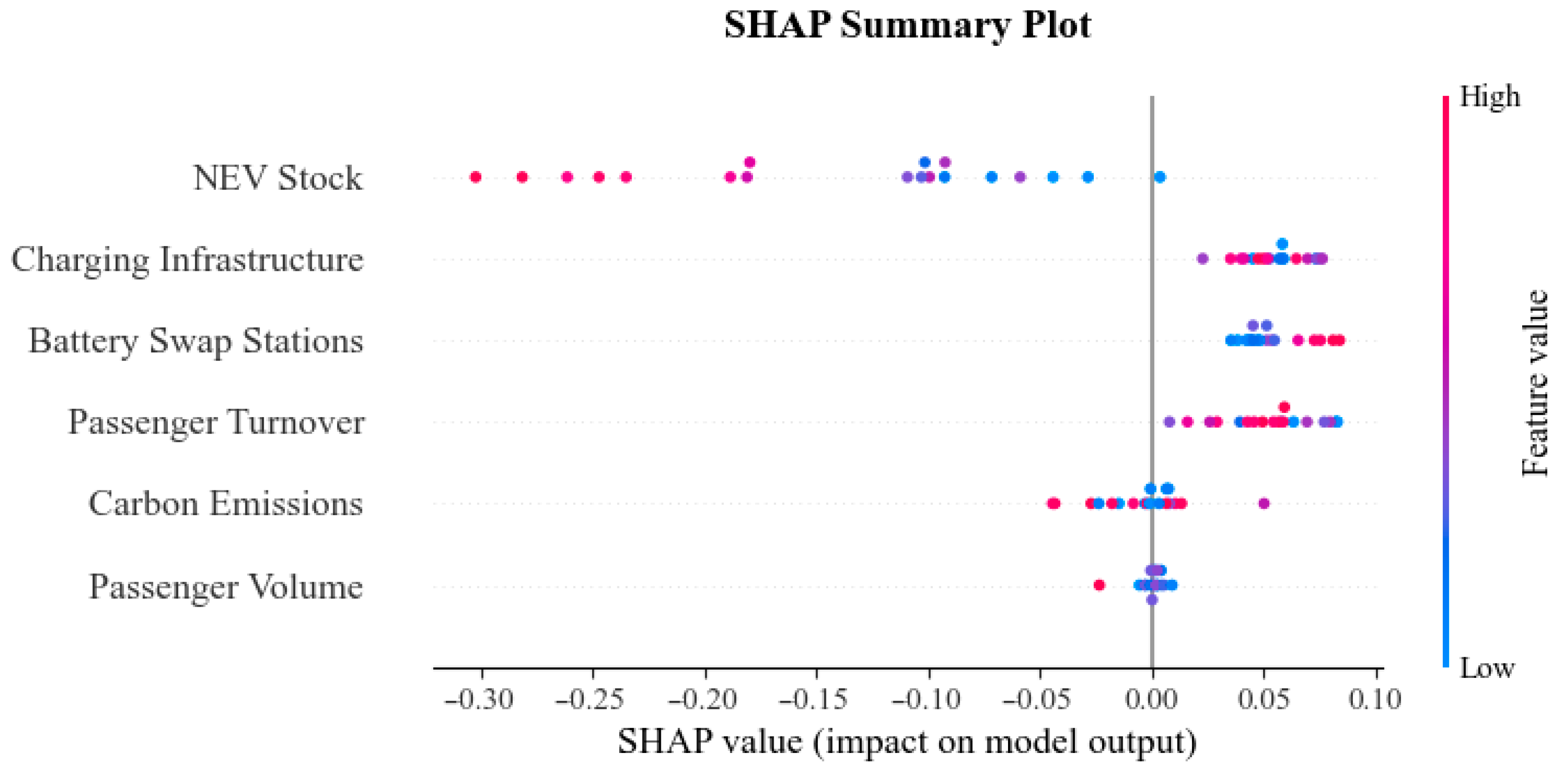
Figure 13 presents the global feature importance analysis based on SHAP values, visualized using a beeswarm plot to comprehensively reflect both the magnitude and direction of each feature’s impact on model predictions. The vertical axis ranks features by importance, with higher-ranking features at the top, while the horizontal axis represents SHAP values (positive values indicate an increase in predicted sales, and negative values indicate a decrease). Color coding denotes the relative feature value, with red representing high values and blue representing low values. From Figure 13, it is evident that NEV Stock exerts the most significant influence on model predictions. Notably, high NEV Stock values (red points) are predominantly located on the negative axis, indicating a marginal growth suppression effect due to market saturation. In contrast, Charging Infrastructure and Battery Swap Stations are primarily distributed along the positive axis, demonstrating that these two types of energy replenishment facilities serve as key positive drivers of NEV sales. SHAP values for Passenger Turnover, Carbon Emissions, and Passenger Volume are largely concentrated near zero, suggesting that these features exhibit relatively low sensitivity in the current predictive model.
It should be noted that certain predictor variables exhibit strong correlations, particularly between Charging Infrastructure and NEV Stock (r = 1.000), as illustrated in Figure 8. This phenomenon is mainly attributed to the coordinated development relationship between NEV deployment and charging infrastructure construction in China. As the number of new energy vehicles increases, charging infrastructure has expanded correspondingly to satisfy charging demand, resulting in a highly synchronized temporal evolution.
Although severe multicollinearity may affect the independent contribution allocation of traditional statistical models, its influence is relatively different in the proposed deep learning-based forecasting framework. The Informer model can capture nonlinear interactions and joint temporal patterns among correlated variables rather than relying on independent parameter estimation. Furthermore, SHAP values in this study are interpreted as feature contributions within the trained model rather than causal effects.
Therefore, the high SHAP importance of NEV Stock and Charging Infrastructure should be understood as their combined contribution to predicting NEV sales trends. The ranking difference between these two variables does not necessarily indicate that one factor completely dominates the other, but rather reflects the model’s allocation of predictive information among correlated features. This consideration has been added to avoid overinterpretation of SHAP-based feature importance results.

4. Discussion

The BAEO–Informer–ARIMA composite forecasting framework developed in this study provides valuable methodological insights for the field of Energy Informatics. Energy Informatics emphasizes the use of data-driven approaches and intelligent algorithms to optimize the configuration and management of energy systems. Forecasting new energy vehicle (NEV) sales represents a critical demand-prediction problem within the broader context of energy consumption structure transformation. By integrating multi-source heterogeneous data—including infrastructure, transportation demand, carbon emissions, and market stock—and combining deep learning with statistical modeling, this study achieves a dynamic characterization of complex energy consumption behaviors. This approach reflects the core paradigm of Energy Informatics: “data fusion → intelligent modeling → decision support”.
In particular, the use of the BAEO algorithm for adaptive hyperparameter optimization enhances prediction accuracy while improving model robustness, providing a generalizable technical framework for addressing high-dimensional, multivariate, and strongly nonlinear forecasting problems in energy systems. Moreover, the incorporation of SHAP-based interpretability analysis offers insights into the intrinsic mechanisms linking energy infrastructure, carbon constraints, and market penetration, supplying transparent and quantifiable evidence to inform energy policy and resource allocation.
Looking forward, NEV sales forecasting can be further extended to broader energy system co-optimization challenges. For example, integrating sales forecasts with electricity load prediction, charging demand response, and renewable energy absorption models could establish a cross-system coupling framework to support coordinated planning of next-generation power and transportation energy systems. Additionally, incorporating higher-frequency data—such as real-time charging behavior or vehicle trajectory information—and scenario simulation methods can enhance the model’s responsiveness to policy interventions and technological innovation. As artificial intelligence becomes increasingly integrated with energy systems, developing dynamic forecasting platforms capable of real-time updates will represent a key direction in Energy Informatics. Overall, this study not only provides empirical support for forecasting China’s NEV market but also offers theoretical and methodological guidance for extending Energy Informatics applications in the context of electrified transportation and low-carbon transition.
Despite the promising forecasting performance achieved by the proposed BAEO–Informer–ARIMA framework, several limitations should be acknowledged. First, although the model was evaluated using an independent test dataset based on chronological splitting, the available historical NEV sales data are still relatively limited. Considering that the NEV market is highly dynamic and strongly influenced by government policies, technological innovation, subsidy adjustments, and infrastructure development, a longer forecasting horizon with additional newly collected data is required to further verify the model’s long-term generalization capability. Future research will focus on continuously updating the dataset, incorporating more comprehensive policy and economic indicators, and conducting rolling forecasting evaluations under different market scenarios. These improvements are expected to further enhance the robustness and practical applicability of the proposed forecasting framework.

5. Conclusions

This study proposed a BAEO–Informer–ARIMA hybrid forecasting framework for China’s new energy vehicle (NEV) sales using multi-source data from 31 provincial-level administrative regions during 2016–2023. By integrating market, infrastructure, transportation, and emission-related factors, the proposed framework effectively captured the complex nonlinear growth patterns and seasonal fluctuations of NEV sales.
The main conclusions are summarized as follows:
(1)
The proposed BAEO–Informer–ARIMA model demonstrated superior forecasting capability compared with conventional statistical models and advanced deep learning approaches, including SARIMA, Prophet, XGBoost, LSTM, GRU, Transformer, and Informer. The results indicate that BAEO optimization improves the representation ability of Informer, while ARIMA residual correction further enhances prediction accuracy and robustness.
(2)
Under a chronological evaluation strategy, the proposed model achieved high prediction accuracy, with an R2 of 0.9544 and a MAPE of 3.39% on the test set, outperforming all benchmark models. These results confirm the effectiveness of combining evolutionary optimization, long-range temporal feature extraction, and residual error correction for NEV sales forecasting.
(3)
The model successfully reproduced the historical growth trajectory and seasonal characteristics of China’s NEV market, capturing rapid market expansion after 2021 as well as periodic fluctuations caused by factors such as holiday effects and annual market cycles. Future projections suggest that NEV sales will maintain sustained growth from 2024 to 2030, although the growth rate is expected to gradually moderate.
(4)
The uncertainty analysis based on forecast errors provided reliable confidence intervals for future predictions, offering additional information for policymakers, infrastructure planners, and industry stakeholders. The proposed framework can serve as an effective decision-support tool for medium- and long-term NEV market planning.
Overall, the BAEO–Informer–ARIMA framework provides an accurate and interpretable approach for NEV sales forecasting by integrating multi-source information and hybrid modeling strategies. Future work will focus on incorporating additional socioeconomic factors, policy changes, and market dynamics to further improve forecasting adaptability under rapidly evolving conditions.

Author Contributions

Conceptualization, S.L. and W.L.; methodology, S.L. and W.L.; software, S.L.; validation, S.L., W.L. and Z.P.; formal analysis, S.L. and W.L.; investigation, S.L.; resources, W.L., Y.L. and Z.P.; data curation, S.L.; writing—original draft preparation, S.L.; writing—review and editing, W.L., Y.L. and Z.P.; visualization, S.L.; supervision, W.L. and Y.L.; project administration, W.L.; funding acquisition, W.L. and Y.L. All authors have read and agreed to the published version of the manuscript.

Funding

This work was supported in part by the Project for Enhancing young and Middle-aged Teacher’s Research Basis Ability in Colleges of Guangxi under Grant 2023KY1080, 2024KY1089 and 2024KY1086.

Data Availability Statement

The datasets analyzed during the current study are publicly available from the China Association of Automobile Manufacturers (CAAM) and related official statistical sources. The processed data used to support the findings of this study are available from the corresponding author upon reasonable request.

Conflicts of Interest

The authors declare no conflicts of interest.

Nomenclature and Abbreviations

The following symbols and abbreviations are used in this manuscript:
AbbreviationFull term
NEVNew Energy Vehicle
BAEOBoomerang Aerodynamic Ellipse Optimizer
ARIMAAuto-Regressive Integrated Moving Average
SARIMASeasonal Auto-Regressive Integrated Moving Average
LSTMLong Short-Term Memory
GRUGated Recurrent Unit
XGBoosteXtreme Gradient Boosting
KCCMean Absolute Error
MAEMean Absolute Error
MSEMean Squared Error
RMSERoot Mean Squared Error
MAPEMean Absolute Percentage Error
R2Coefficient of Determination
SHAPSHapley Additive exPlanations
MLPMulti-Layer Perceptron
RNNRecurrent Neural Network
SVRSupport Vector Regression
RFRandom Forest Regression
ProphetProphet

References

  1. Issakhov, A.; Omarova, P. Modeling and analysis of the effects of barrier height on automobiles emission dispersion. J. Clean. Prod. 2021, 296, 126450. [Google Scholar] [CrossRef] [Scilit]
  2. Ahmed, Z.; Cary, M.; Le, H.P. Accounting asymmetries in the long-run nexus between globalization and environmental sustainability in the United States: An aggregated and disaggregated investigation. Environ. Impact Assess. Rev. 2021, 86, 106511. [Google Scholar] [CrossRef] [Scilit]
  3. Avetisyan, M.; Hertel, T.; Sampson, G. Is local food more environmentally friendly? The GHG emissions impacts of consuming imported versus domestically produced food. Environ. Resour. Econ. 2014, 58, 415–462. [Google Scholar] [CrossRef] [Scilit]
  4. Qi, S. Factors Influencing the Consumption Behavior Towards New Energy Vehicles (Nev) in Japan. Ph.D. Thesis, Waseda University, Tokyo, Japan, 2022. [Google Scholar]
  5. Azar, C.; Lindgren, K.; Andersson, B.A. Global energy scenarios meeting stringent CO2 constraints—Cost-effective fuel choices in the transportation sector. Energy Policy 2003, 31, 961–976. [Google Scholar] [CrossRef] [Scilit]
  6. Halff, A.; Younes, L.; Boersma, T. The likely implications of the new IMO standards on the shipping industry. Energy Policy 2019, 126, 277–286. [Google Scholar] [CrossRef] [Scilit]
  7. Ning, T.; Lu, B.; Ouyang, X.; Ouyang, H.; Chen, J. Prospect and sustainability prediction of China’s new energy vehicles sales considering temporal and spatial dimensions. J. Clean. Prod. 2024, 468, 142926. [Google Scholar] [CrossRef] [Scilit]
  8. Li, B. Industrial Policy and Enlightenments: Analysis of China’s New Energy Vehicle Industry. 2024. Available online: https://ssrn.com/abstract=5171262 (accessed on 23 July 2026).
  9. Li, Y.; Zhang, L.; Liu, J.; Qiao, X. Can the dual-credit policy help china’s new energy vehicle industry achieve corner overtaking? Sustainability 2023, 15, 2406. [Google Scholar] [CrossRef] [Scilit]
  10. Tanmayi, G.; Radha, R.; Sai Varshitha, U.V.; Prakash, P.A. Leveraging deep transfer learning and adaptive power models for enhanced charging time prediction in electric vehicles. Energy Inform. 2025, 8, 110. [Google Scholar] [CrossRef] [Scilit]
  11. Resch, G.; Liebmann, L.; Geipel, J.; Wien, F.H.T.; Hendricks, D.; Vollmer, J.; Fouquet–EREF, D. Study on 2030 Renewable Energy and Energy Efficiency Targets in the European Union; European Renewable Energies Federation: Brussels, Belgium, 2023. [Google Scholar]
  12. Huang, Y.; Yang, J.; Liu, C.; Jing, R.; Lu, Q. Spatial and Temporal Variations in Rainwater Chemistry in a Rapid Urbanization Area of Shenzhen, China. Atmosphere 2024, 15, 1536. [Google Scholar] [CrossRef] [Scilit]
  13. Shi, L.; Fu, Z.; Guo, W.; Zhang, J.; Sun, J. Exploring the Factors That Promote Sustainable Growth in Regional Sales of New Energy Vehicles: An Empirical Study of China. Sustainability 2023, 15, 6748. [Google Scholar] [CrossRef] [Scilit]
  14. Rao, Y. New energy vehicles and sustainability of energy development: Construction and application of the Multi-Level Perspective framework in China. Sustain. Comput. Inform. Syst. 2020, 27, 100396. [Google Scholar] [CrossRef] [Scilit]
  15. Yuan, X.; Liu, X.; Zuo, J. The development of new energy vehicles for a sustainable future: A review. Renew. Sustain. Energy Rev. 2015, 42, 298–305. [Google Scholar] [CrossRef] [Scilit]
  16. Liu, L.; Liu, S.; Wu, L.; Zhu, J.; Shang, G. Forecasting the development trend of new energy vehicles in China by an optimized fractional discrete grey power model. J. Clean. Prod. 2022, 372, 133708. [Google Scholar] [CrossRef] [Scilit]
  17. Rietmann, N.; Hügler, B.; Lieven, T. Forecasting the trajectory of electric vehicle sales and the consequences for worldwide CO2 emissions. J. Clean. Prod. 2020, 261, 121038. [Google Scholar] [CrossRef] [Scilit]
  18. Tang, L.; Sun, J. Predict the sales of New-energy Vehicle using linear regression analysis. In Proceedings of the E3S Web of Conferences, Shanghai, China, 16–18 August 2019; EDP Sciences: Les Ulis, France, 2019; p. 02076. [Google Scholar]
  19. Wang, S. Exploring the sustainability of China’s new energy vehicle development: Fresh evidence from population symbiosis. Sustainability 2022, 14, 10796. [Google Scholar] [CrossRef] [Scilit]
  20. Kamis, A.; Abraham, P.S. Predictive models of electric vehicle adoption in the United States: Charging ahead with renewable energy. Transp. Res. Interdiscip. Perspect. 2024, 24, 101041. [Google Scholar] [CrossRef] [Scilit]
  21. Chen, D. Chinese automobile demand prediction based on ARIMA model. In Proceedings of the 2011 4th International Conference on Biomedical Engineering and Informatics (BMEI), Shanghai, China, 15–17 October 2011; IEEE: New York, NY, USA, 2011; pp. 2197–2201. [Google Scholar]
  22. Luo, W.; Deng, J.; Zhou, T.; Xu, R. Research on the Development of New Energy Vehicles and the Prediction of Carbon Emissions in a Region of Asia. In Proceedings of the 2023 International Conference on Network, Multimedia and Information Technology (NMITCON), Bengaluru, India, 1–2 September 2023; IEEE: New York, NY, USA, 2023; pp. 1–7. [Google Scholar]
  23. Du, Y.; Wei, K.; Wang, Y.; Jia, J. New energy vehicles sales prediction model combining the online reviews sentiment analysis: A case study of Chinese new energy vehicles market. In Proceedings of the Artificial Intelligence in China: Proceedings of the 3rd International Conference on Artificial Intelligence in China, Changbaishan, China, 22–23 October 2022; Springer: Singapore, 2022; pp. 424–431. [Google Scholar]
  24. Shahin, M.; Chen, F.F.; Maghanaki, M.; Firouzranjbar, S.; Hosseinzadeh, A. Evaluating the fidelity of statistical forecasting and predictive intelligence by utilizing a stochastic dataset. Int. J. Adv. Manuf. Technol. 2025, 138, 193–223. [Google Scholar]
  25. Sakib, M.; Mustajab, S.; Alam, M. Ensemble deep learning techniques for time series analysis: A comprehensive review, applications, open issues, challenges, and future directions. Clust. Comput. 2025, 28, 73. [Google Scholar]
  26. Al-Mahdi, I.; Darwish, S.; Madbouly, M. Heart disease prediction model using feature selection and ensemble deep learning with optimized weight. Comput. Model. Eng. Sci. 2025, 143, 875. [Google Scholar] [CrossRef] [Scilit]
  27. Bilal, O.; Hekmat, A.; Shahzad, I.; Raza, A.; Khan, S.U.R. Boosting Machine Learning Accuracy for Cardiac Disease Prediction: The Role of Advanced Feature Engineering and Model Optimization. Rev. Socionetwork Strateg. 2025, 19, 271–300. [Google Scholar] [CrossRef] [Scilit]
  28. Zhao, S.; Meng, F.; Cai, L.; Yang, R. Boomerang aerodynamic ellipse optimizer: A human game-inspired optimization technique for numerical optimization and multilevel thresholding image segmentation. Math. Comput. Simul. 2025, 238, 604–636. [Google Scholar] [CrossRef] [Scilit]
  29. Lan, H.; Lu, H.; Wu, Y.; Qin, R.; Tao, S.; Huang, H.; Zhang, S. Application of Informer model based on dual probsparse self-attention mechanism and temporal feature decoder in PEMFC degradation prediction. Energy Convers. Manag. 2026, 348, 120737. [Google Scholar] [CrossRef] [Scilit]
  30. Jin, Z.; Fu, X.; Xiang, L.; Zhu, G.; Hu, A. Informer learning framework based on secondary decomposition for multi-step forecast of ultra-short term wind speed. Eng. Appl. Artif. Intell. 2025, 139, 109702. [Google Scholar] [CrossRef] [Scilit]
  31. Kuang, D.; Wang, Z.; Zhao, Y.; Li, L. Estimating the health status of lithium-ion batteries using deep learning method based on informer model. J. Power Sources 2025, 645, 237176. [Google Scholar] [CrossRef] [Scilit]
  32. Wang, L.; Chen, L.; Jin, S.; Li, C. Forecasting the green behaviour level of Chinese enterprises: A conjoined application of the autoregressive integrated moving average (ARIMA) model and multi-scenario simulation. Technol. Soc. 2025, 81, 102825. [Google Scholar] [CrossRef] [Scilit]
  33. Gong, X.; Li, B.; Yang, Y.; Li, M.; Li, T.; Zhang, B.; Zheng, L.; Duan, H.; Liu, P.; Hu, X. Construction and application of optimized model for mine water inflow prediction based on neural network and ARIMA model. Sci. Rep. 2025, 15, 2009. [Google Scholar] [CrossRef] [Scilit] [PubMed]
  34. Yearbook, C.S. China Statistical Yearbook; Zhongguo Tongji Chubanshe: Beijing, China, 2014. [Google Scholar]
  35. Wu, S.; Yang, Z. Availability of public electric vehicle charging pile and development of electric vehicle: Evidence from China. Sustainability 2020, 12, 6369. [Google Scholar] [CrossRef] [Scilit]
  36. Tarkhov, S. Geography of the passenger turnover dynamics at airports in Europe and Russia’s regions in the first year of the COVID-19 pandemic. Reg. Res. Russ. 2021, 11, 435–453. [Google Scholar] [CrossRef] [Scilit]
  37. Huang, R.; Zhang, S.; Wang, P. Key areas and pathways for carbon emissions reduction in Beijing for the “Dual Carbon” targets. Energy Policy 2022, 164, 112873. [Google Scholar] [CrossRef] [Scilit]
  38. Yang, H.; Wang, H.; Gao, Y.; Liu, X.; Xu, M. A significant wave height forecast framework with end-to-end dynamic modeling and lag features length optimization. Ocean Eng. 2022, 266, 113037. [Google Scholar] [CrossRef] [Scilit]
  39. Wang, Z.; Yang, J.; Guo, Y. Unknown fault feature extraction of rolling bearings under variable speed conditions based on statistical complexity measures. Mech. Syst. Signal Process. 2022, 172, 108964. [Google Scholar] [CrossRef] [Scilit]
  40. Lach, J. Analysis of the Differences Resulting from the Determination of Langmuir Isotherm Coefficients from Linear and Non-Linear Forms—A Case Study. Materials 2025, 18, 3506. [Google Scholar] [CrossRef] [Scilit] [PubMed]
  41. Camarillo-Cisneros, J.; Ramirez-Alonso, G.; Arzate-Quintana, C.; Varela-Rodríguez, H.; Guzman-Pando, A. MolGC: Molecular geometry comparator algorithm for bond length mean absolute error computation on molecules. Mol. Divers. 2024, 28, 1925–1945. [Google Scholar] [CrossRef] [Scilit] [PubMed]
  42. Karunasingha, D.S.K. Root mean square error or mean absolute error? Use their ratio as well. Inf. Sci. 2022, 585, 609–629. [Google Scholar] [CrossRef] [Scilit]
  43. Takyi-Aninakwa, P.; Wang, S.; Zhang, H.; Li, H.; Xu, W.; Fernandez, C. An optimized relevant long short-term memory-squared gain extended Kalman filter for the state of charge estimation of lithium-ion batteries. Energy 2022, 260, 125093. [Google Scholar] [CrossRef] [Scilit]
  44. Mangalathu, S.; Hwang, S.-H.; Jeon, J.-S. Failure mode and effects analysis of RC members based on machine-learning-based SHapley Additive exPlanations (SHAP) approach. Eng. Struct. 2020, 219, 110927. [Google Scholar] [CrossRef] [Scilit]
Figure 1. Mapping Process.
Wevj 17 00404 g001
Figure 2. ARIMA Model Structure.
Wevj 17 00404 g002
Figure 3. Combined Model Prediction Process.
Wevj 17 00404 g003
Figure 4. Visualization of Lag Characteristics, Moving Average Characteristics, and Seasonal Cycle Characteristics. (a) Lag Characteristics: Historical Sales (1–6 months), (b) Moving Average Characteristics (MA3/MA6/MA12), (c) Moving Standard Deviation Characteristics (3-month window), (d) Seasonal Cycle Characteristics (Monthly Sine and Cosine Transforms), (e) Polar Radar Chart: Seasonal Cycle Characteristics of Monthly Average Sales.
Wevj 17 00404 g004
Figure 5. Monthly Sales Volume and Growth Rate of New Energy Vehicles.
Wevj 17 00404 g005
Figure 6. Comparison of Total Sales Volume Across Chinese Provinces, 2016–2023.
Wevj 17 00404 g006
Figure 7. Regional Heat Map of Total Sales Volume by Province, 2016–2023.
Wevj 17 00404 g007
Figure 8. Correlation Thermogram. Note: ** p < 0.01, *** p < 0.001
Wevj 17 00404 g008
Figure 9. Parameter Iteration Diagram.
Wevj 17 00404 g009
Figure 10. Comparison of Predicted and Actual Monthly NEV Sales Volumes in the Training Set and the Representative Test Window (January–November 2023).
Wevj 17 00404 g010
Figure 11. Forecast Results for 2024–2030.
Wevj 17 00404 g011
Figure 12. Provincial NEV Sales Forecasts from 2024 to 2030 Using the Unified BAEO–Informer–ARIMA Framework.
Wevj 17 00404 g012
Figure 13. SHAP Global Feature Importance Analysis.
Wevj 17 00404 g013
Table 1. BAEO Hyperparameter Optimization Results.
HyperparametersSearch ScopeOptimum Value
Learning Rate[0.001, 0.005]0.001083
Hidden Size[96, 232]190
Sequence Length[1, 7]1
Batch Size[8, 20]19
Dropout Rate[0.15, 0.35]0.179
Validation MSE-0.004432
Table 2. Model Evaluation Metrics.
DatasetR2MAPE (%)MAERMSE
Training Set0.97983.475510,945.415,423.41
Test Set0.95443.389924,068.328,621.54
Table 3. Performance Comparison of Prediction Results Across Different Models.
MethodR2MSEMAERMSE
Training SetTest SetTraining SetTest SetTraining SetTest SetTest SetTraining Set
Informer0.94910.9022601,303,040742,910,23118,800.6424,500.5424,521.4828,017.87
ARIMA0.66920.61543,910,822,7284,052,991,48244,780.8748,900.2162,536.5764,807.44
Informer-ARIMA0.97330.9381314,975,456389,120,55112,537.0816,200.4517,747.5921,213.26
BAEO–Informer0.95910.9157483,982,752558,201,39416,376.4320,100.8921,999.6124,899.84
BAEO–Informer–ARIMA0.97980.9544230,113,468269,452,10810,945.3924,068.2915,423.4228,621.54
Table 4. Extended Baseline Comparison on the Test Set.
ModelR2 (Test)MAE (Test)RMSE (Test)MAPE (%)
SARIMA0.842747,86059,4208.74
Prophet0.861944,73055,6808.05
XGBoost0.901636,54045,8706.43
LSTM0.914233,26041,9305.78
GRU0.923731,18039,2405.31
Transformer0.935128,94035,7604.62
Informer0.902224,50128,0174.07
BAEO–Informer–ARIMA0.954424,06826,8223.39
Disclaimer/Publisher’s Note: The statements, opinions and data contained in all publications are solely those of the individual author(s) and contributor(s) and not of MDPI and/or the editor(s). MDPI and/or the editor(s) disclaim responsibility for any injury to people or property resulting from any ideas, methods, instructions or products referred to in the content.