Thermal Management of a Zero-Emission Magnetorheological Braking: CFD Evaluation of Liquid-Cooling Strategies

Abstract

MagnetoRheological Brakes (MRBs) can provide wear-free, electrically controllable braking torque, but repeated high-load braking can cause rapid heat accumulation in the narrow rotor–stator gap and degrade MRF performance. This study evaluates rotor-only, stator-only and combined rotor–stator liquid-cooling configurations using transient 3-D conjugate heat-transfer CFD in ANSYS Fluent 2024 R1 for a UN Regulation No. 13-H-based 10-cycle duty profile (8.5 s acceleration, 20 s constant speed and 2.5 s braking per cycle). The activated MRF is modeled as an incompressible laminar Herschel–Bulkley fluid during braking, while the field-OFF phases use a Newtonian viscosity of 0.114 Pa·s; viscous dissipation and coil volumetric heating are included as internal heat sources. Cooling simulations apply water with a 130 kPa (absolute) inlet pressure and a conservative +20% heat-load margin with adiabatic external boundaries. Baseline uncooled dynamometer data (no integrated cooling) verify the thermal implementation, with a 7.06% underprediction of the measured temperature rise. In the uncooled case, the MRF reaches a temperature of 501 K after ten cycles; rotor-only and stator-only cooling reduce temperatures but do not fully suppress cumulative heating, whereas the combined configuration maintains the MRF below 400 K after ten cycles. These results indicate that cooling both dominant heat paths is required for stable MRB thermal operation under severe repeated braking.

1. Introduction

Brake-wear particulate emissions (“brake dust”) are increasingly discussed as an important non-exhaust source of traffic-related PM. As tailpipe emissions decrease, the relative impact of braking-generated particles becomes more visible, and regulations such as Euro 7 are pushing the community toward brake systems that reduce wear and thermal stress. A recent review summarizes the contribution of braking emissions and the mitigation strategies being considered [1,2].

Regenerative braking (RB) is a key technology in electric and hybrid vehicles because it recovers kinetic energy during deceleration and improves overall energy efficiency, reducing the PM generated [3,4]. However, RB cannot always satisfy the full braking demand, particularly at low vehicle speed or when the battery state-of-charge limits the allowable charging power. Therefore, conventional friction braking remains necessary to ensure safe operation under all driving conditions [5,6,7]. Under repeated or severe braking, friction systems also face thermal fade due to heat accumulation, in addition to brake-wear PM emissions [8,9,10,11,12,13].

In the Zero-Emissions Driving System (ZEDS) concept, a MagnetoRheological Fluid Brake (MRB) is proposed as a torque actuator that can be modulated electrically without sliding contact to substitute standard disk brakes. When a magnetic field is applied, the MagnetoRheological Fluid (MRF) exhibits an increased resistance to shear (yield stress and apparent viscosity), enabling controllable braking torque generation in a narrow active gap. This approach can reduce reliance on friction braking during many operating conditions and supports integration with brake-by-wire control architectures [2,8,14].

The design concept in Figure 1 and

Table 1. List of Components Corresponding to Figure 1.

Part Number	Part
1	Rotor of electric motor
2	Stator of electric motor
3	Stator of brake system
4	Extended rotor from Electric motor
5	Coils

integrates an in-wheel electric motor with an external braking stator, using MRF to generate resistive braking torque in the rotor–stator active region. The rotor includes an extension that protrudes into the stator to define the active gap, while the stator geometry is shaped to provide braking surface area within the packaging constraints of the suspension region. A coil located on the outer clamp generates the magnetic field required for MRF activation [2,8,14].

A primary challenge for MRB implementation in this architecture is thermal management. Under severe braking, heat generation is concentrated in the MRF gap due to shear heating during magnetic activation, and the coil contributes additional Joule losses. Because the gap is thin and the surrounding metal components provide limited heat capacity and conduction paths, the brake can exhibit cumulative temperature rise over repeated cycles, which may degrade MRF performance and accelerate fluid aging [8,15]. This motivates a transient conjugate heat-transfer analysis capable of resolving heat generation in the gap and heat rejection through the rotor/stator structures.

Several cooling approaches have been adopted in braking and high-heat rotating systems. Air cooling (natural or forced convection) is widely used and can be enhanced through ventilated discs, ducts, or fins, but may be insufficient for severe duty cycles [16,17,18,19,20,21].

Liquid cooling provides higher heat rejection through internal coolant passages and is commonly applied in high-load systems, with the trade-off of added plumbing and pumping requirements [18,22,23,24,25,26]. Passive or hybrid approaches such as Phase-change materials (PCMs) for transient heat buffering and heat pipes for passive heat spreading have also been investigated, often as supplements to other cooling methods [18,27,28,29].

To provide a clearer quantitative comparison with previous liquid-cooled magnetorheological systems,

Table 2. Quantitative comparison with prior liquid-cooled magnetorheological braking and torque-transfer systems.

Study	System and Cooling Strategy	Reported Metrics
[22]	Multi-disc MR brake with inner water-cooling channels	${\mathrm{M}}_{\mathrm{m}\mathrm{a}\mathrm{x}}=96.24$ N·m$; \mathrm{after} 20 \mathrm{s} \mathrm{braking}, \mathrm{torque} \mathrm{reduction} \mathrm{decreased} \mathrm{from} 25.1\%$$\mathrm{without} \mathrm{cooling} \mathrm{to} 20\%$ with cooling
[23]	High-torque MR brake with water cooling	${\mathrm{M}}_{\mathrm{M}\mathrm{a}\mathrm{x}}=980$ N·m$,$$\mathrm{over} 90 \mathrm{s}, \mathrm{torque} \mathrm{reduction} \mathrm{decreased} \mathrm{from} 12.1\%$$\mathrm{under} \mathrm{natural} \mathrm{cooling} \mathrm{to} 2.4\%$$\mathrm{with} \mathrm{water} \mathrm{cooling} \mathrm{at} \mathrm{Q}=15\hspace{0.17em}\mathrm{L}/\mathrm{m}\mathrm{i}\mathrm{n}$
[26]	Liquid-cooled MR clutch	$\mathrm{Allowable} \mathrm{steady} \mathrm{slip} \mathrm{power} 35\hspace{0.17em}\mathrm{k}\mathrm{W}$$; \mathrm{allowable} \mathrm{transient} \mathrm{slip} \mathrm{power} 53.2\hspace{0.17em}\mathrm{k}\mathrm{W}$$\mathrm{for} 120\hspace{0.17em}\mathrm{s}$
Present Study	In-wheel EV MR brake with rotor-only, stator-only, and combined rotor–stator liquid cooling	$\mathrm{Phase}-\mathrm{equivalent} \mathrm{braking} \mathrm{torque} \approx 933\hspace{0.17em}\mathrm{N}\cdot \mathrm{m};$$\mathrm{braking}-\mathrm{phase} \mathrm{thermal} \mathrm{load} 57.24\hspace{0.17em}\mathrm{k}\mathrm{W};$$\mathrm{combined} \mathrm{cooling} \mathrm{keeps} \mathrm{volume}-\mathrm{averag} \mathrm{MRF} \mathrm{below} 400\hspace{0.17em}\mathrm{K}$$\mathrm{after} 10 \mathrm{cycles}, \mathrm{compared} \mathrm{with} \approx 501\hspace{0.17em}\mathrm{K}$ uncooled

summarizes representative studies for which directly comparable quantitative metrics were available. The comparison includes liquid-cooled MR brakes and MR torque-transfer devices and focuses on the device type, cooling strategy, reported performance metrics, and relevance to the present work.

For the present study, $M_{\mathrm{e}\mathrm{q}}$ is the phase-equivalent mechanical braking torque calculated from the MRF gap dissipation during the imposed braking ramp; it is not an instantaneous maximum torque.

Table 2 focuses on studies with directly comparable quantitative metrics; additional liquid-cooled braking and MR torque-transfer studies [24,25] are discussed in the surrounding literature. Compared with the studies summarized in Table 2, the present work is distinguished by comparing rotor-only, stator-only, and combined rotor–stator cooling under the same repeated-braking duty cycle.

Given the localized and repeated thermal loading of the MRB gap region, this research focuses on liquid cooling as the primary strategy for sustained heat removal. In particular, two liquid-cooling concepts are evaluated. First, rotor cooling channels are designed to exploit centrifugal effects in rotating passages, with the objective of increasing coolant flow at higher rotational speeds and potentially reducing pump demand. Second, stator cooling channels are designed for stable coolant distribution and heat extraction on the stationary side of the brake. The cooling concepts are evaluated using transient three-dimensional CFD (ANSYS Fluent 2024 R1) under a UN Regulation No. 13-H-based repeated braking waveform [30], with mesh and time-step studies to support numerical reliability and a baseline experimental verification in the uncooled configuration to check the heat generation and boundary condition implementation.

2. Materials and Methods

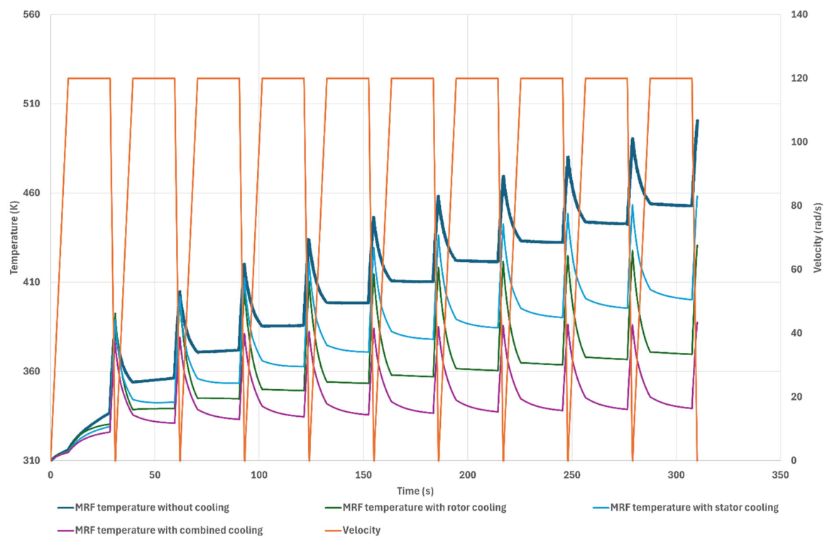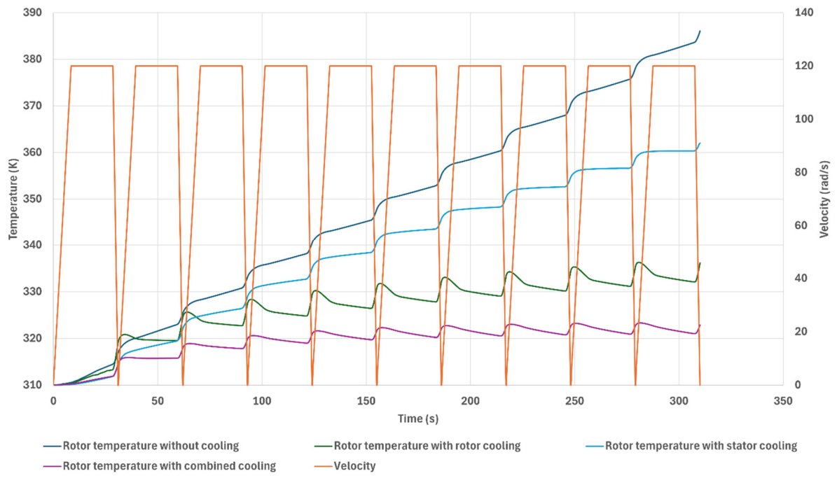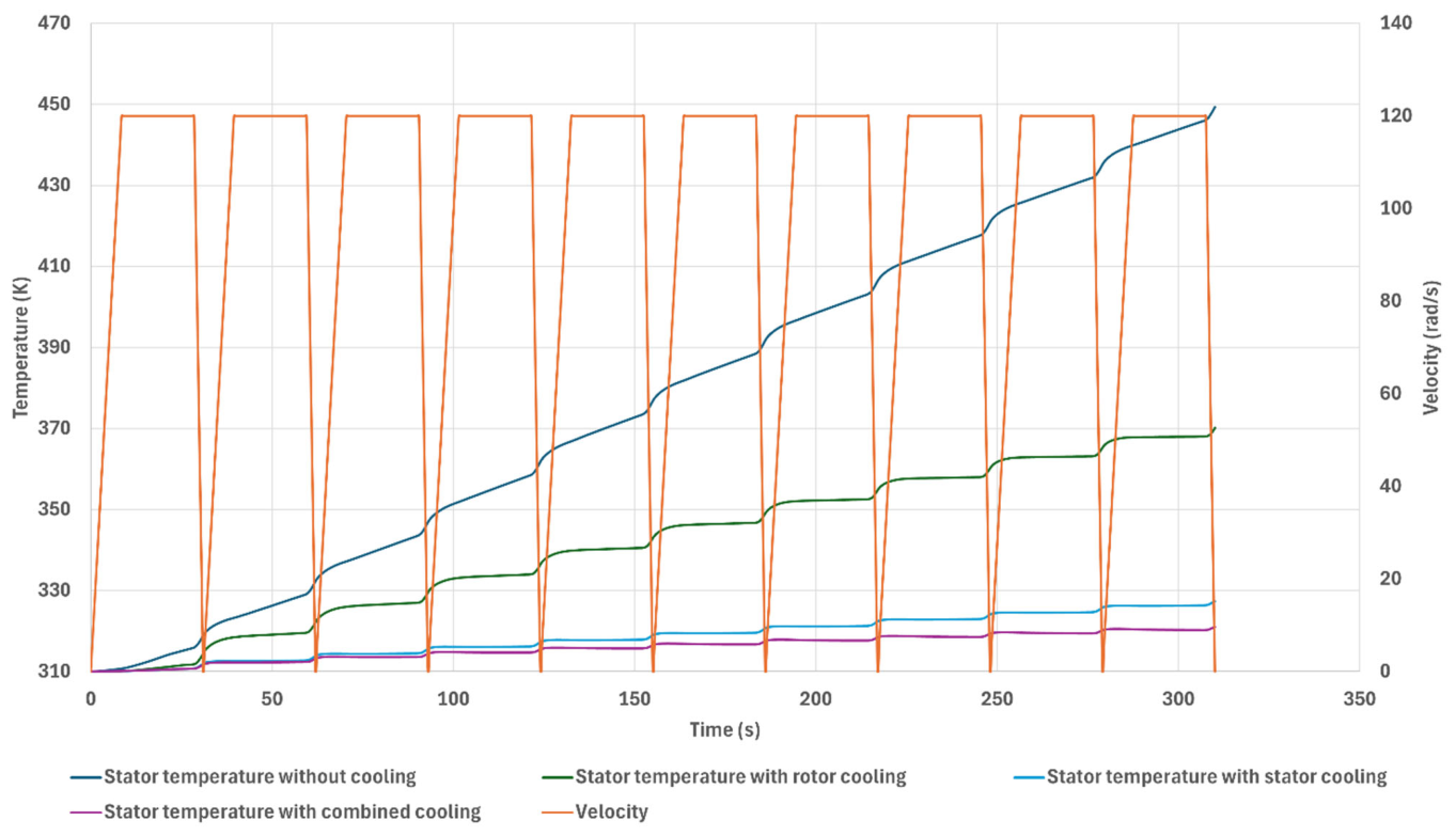
2.1. Computational Domain and Boundary Conditions

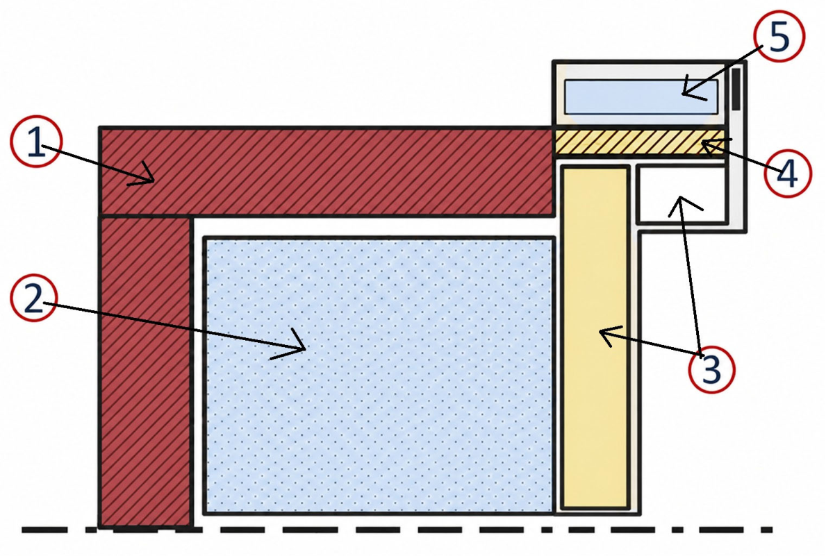
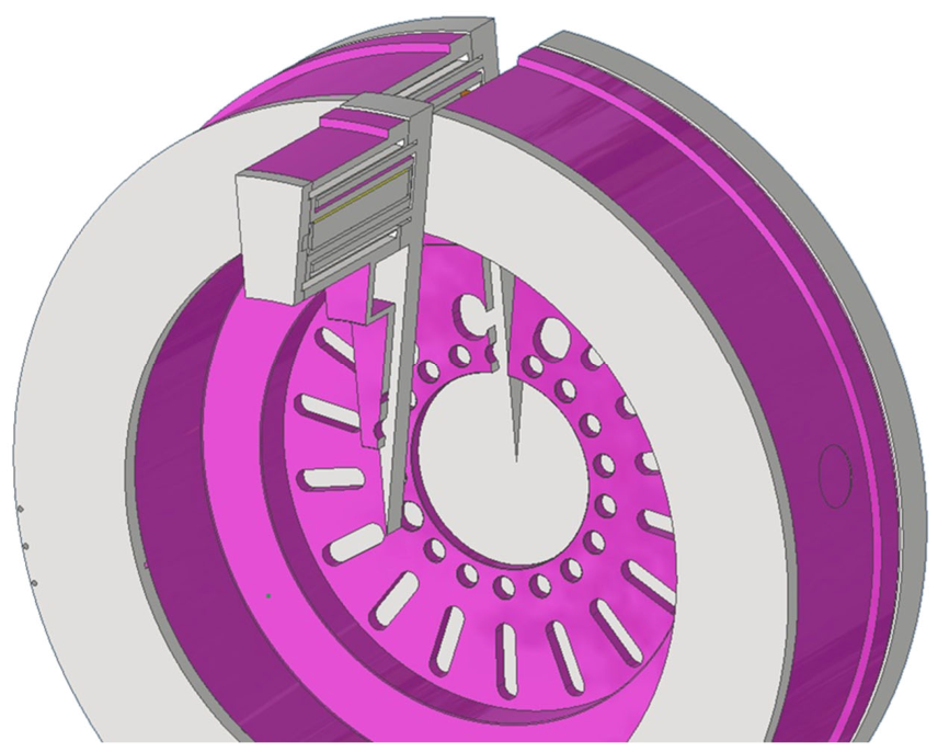
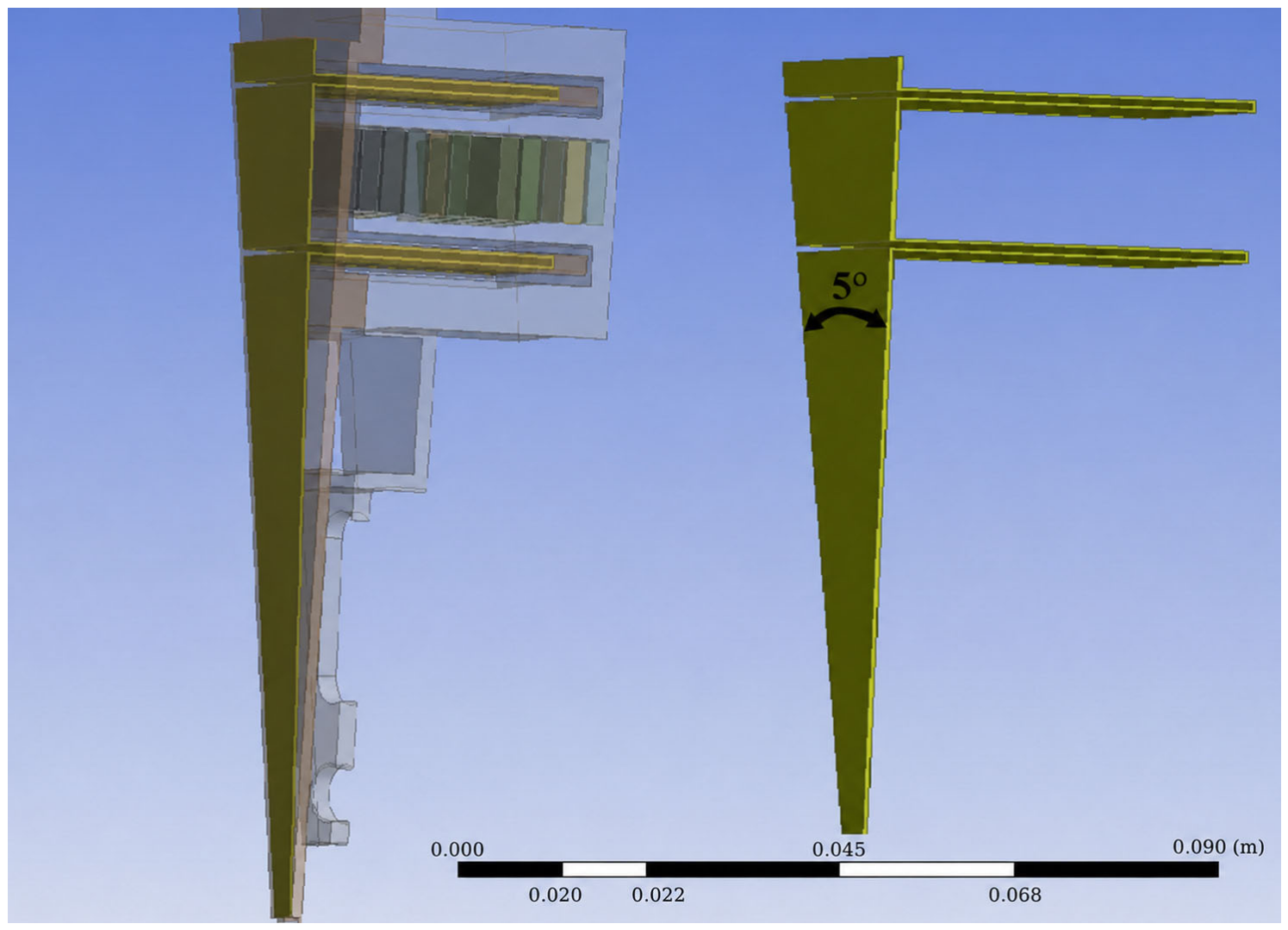
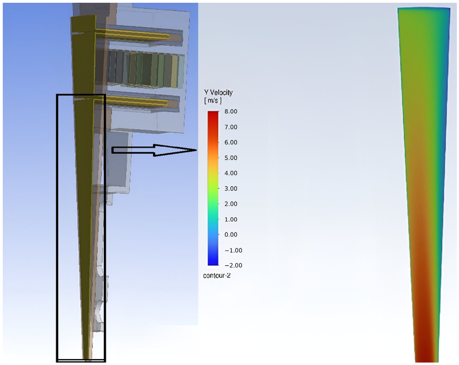
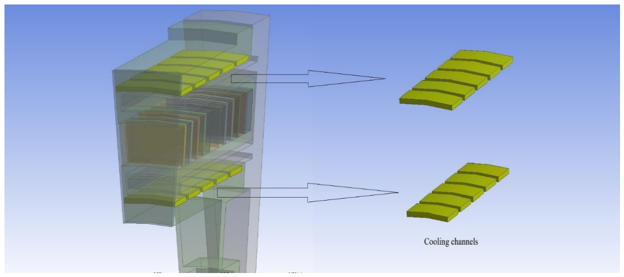
To reduce computational cost while preserving the dominant thermal and flow physics, the transient thermal/conjugate-heat-transfer simulations were conducted on a 5° angular sector of the full 360° geometry (Figure 2). This computational sector should not be confused with the full angular pitch of the rotor cooling-channel layouts discussed in Section 3.3, where the 5° value refers to the cooling passage aperture rather than the complete pitch.

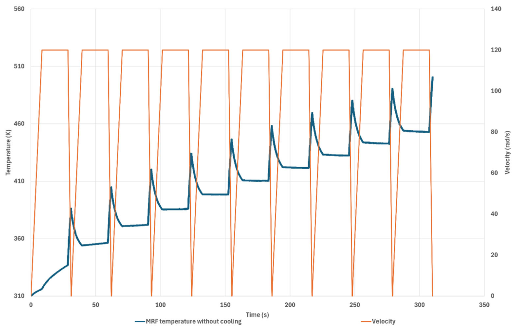
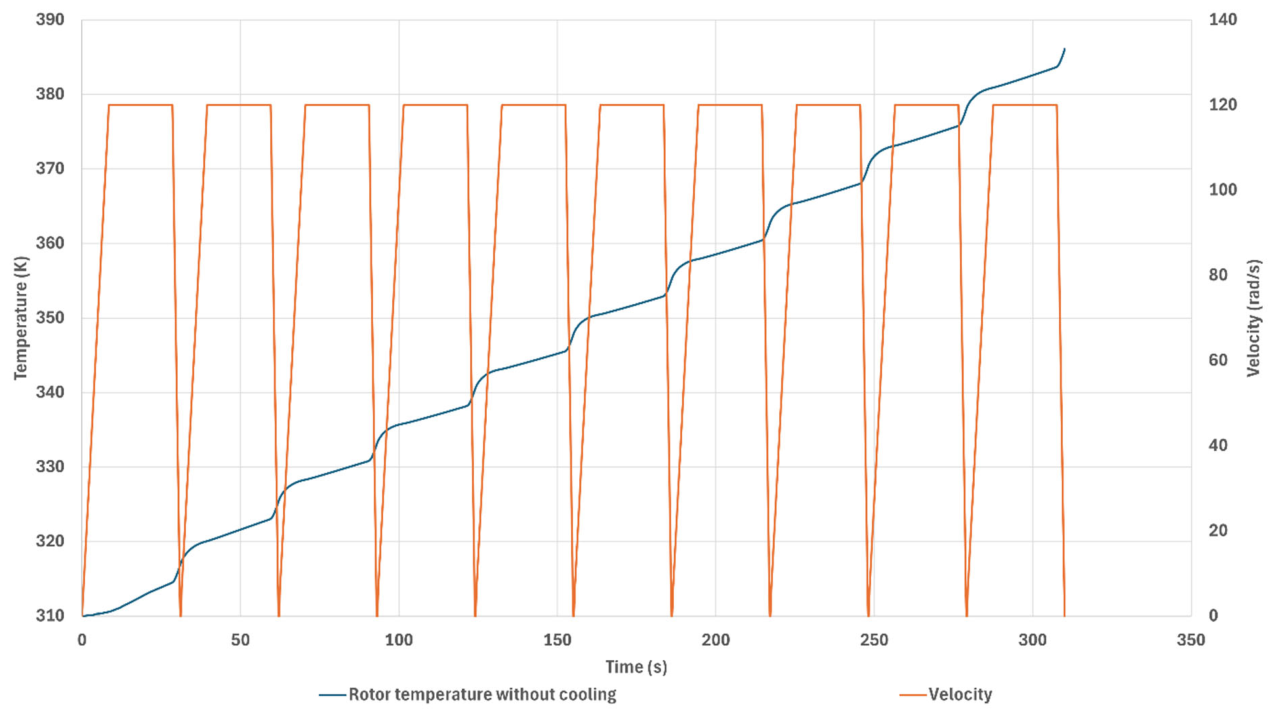
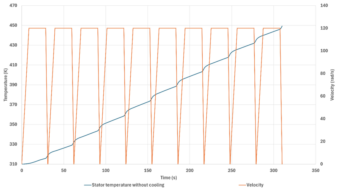
The simulation addresses three key phases within 10 operational cycles following the UN Regulation No 13-H—Uniform provisions concerning the approval of passenger cars with regard to braking [30]:

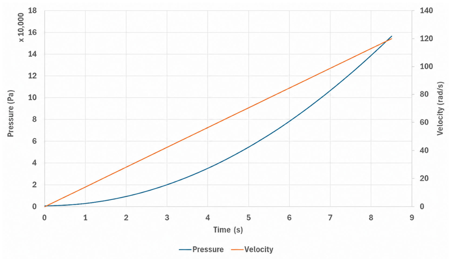
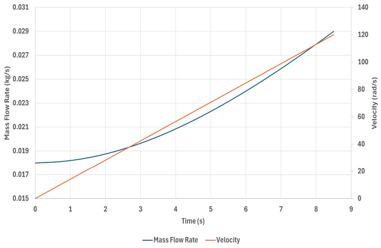
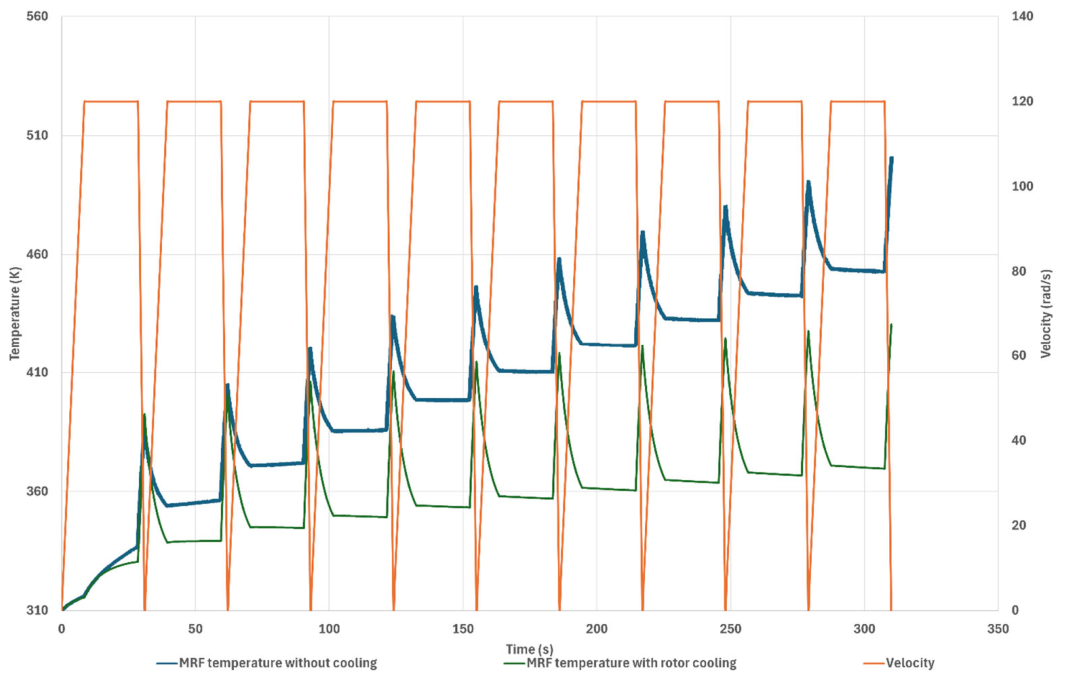
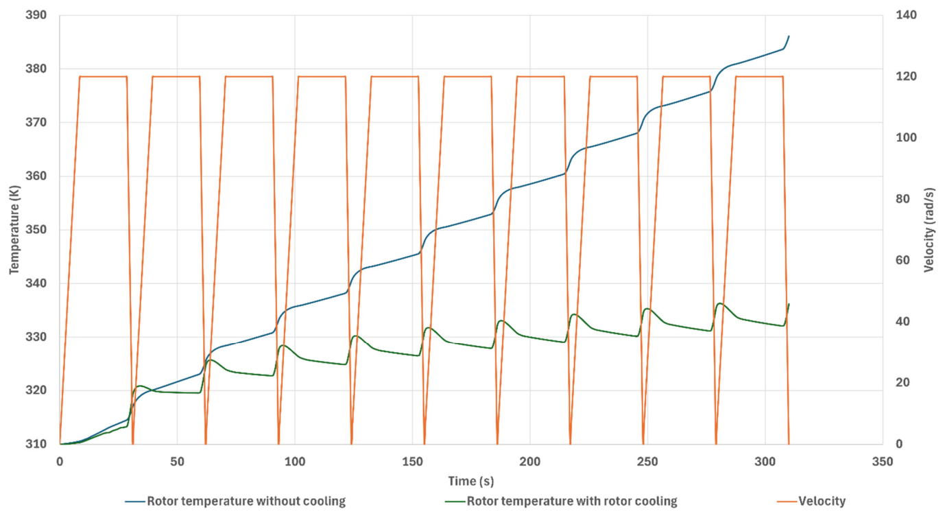
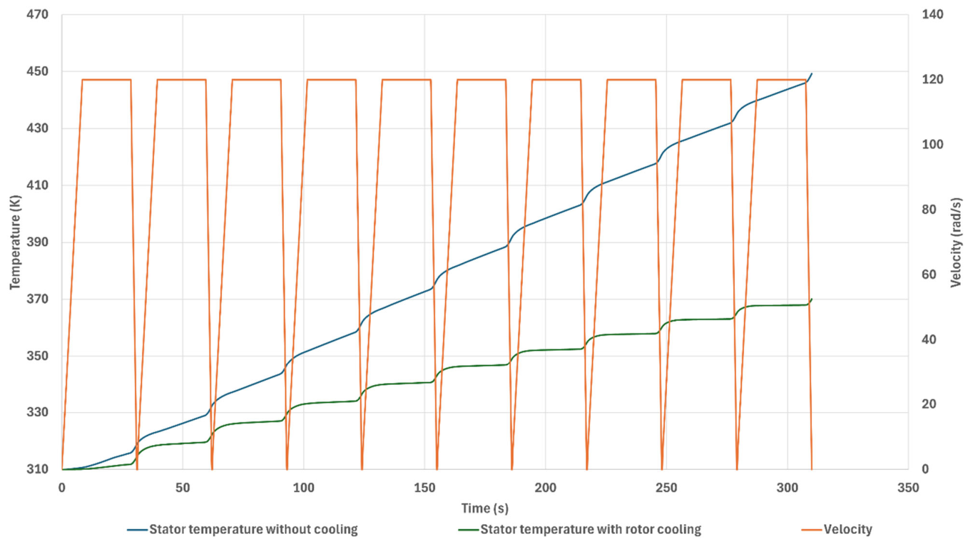
• Acceleration Phase (8.5 s): the rotor accelerates from 0 to 120 rad/s with the magnetic field inactive; the MRF is modeled in its field-OFF Newtonian state.
• Constant-Speed Phase (20 s): the rotor maintains a constant angular speed with the magnetic field inactive; the MRF remains in its field-OFF Newtonian state.
• Deceleration Phase (2.5 s): the magnetic field is activated (field-ON), increasing the MRF resistance to shear (yield stress and apparent viscosity), thereby generating braking torque as the rotor decelerates.

The imposed duty cycle is summarized in

Table 3. Duty-cycle definition used in CFD (UN R13-H-based waveform).

Cycle Phase	Magnetic State	Rotor Speed Definition ω (rad/s)	Duration (s)
Acceleration	Field-OFF	0 → 120	8.5
Constant speed	Field-OFF	120	20
Deceleration	Field-ON	120 → 0	2.5

, including the phase durations used to define $\omega \left(t\right)$ and magnetic actuation scheduling.

During braking, the magnetorheological fluid (MRF) in the rotor–stator gap was modeled as an incompressible, laminar yield-stress non-Newtonian fluid using the Herschel–Bulkley (H–B) constitutive law [31]. In terms of shear stress magnitude $\tau$ and shear-rate magnitude $\dot{\gamma }$, the activated MRF response is:

$$\tau ={\tau }_y+K {\dot{\gamma }}^n,$$

(1)

where ${\tau }_y$ is the field- dependent yield stress, $K$ is the consistency index, and $n$ is the flow-behavior index (temperature dependence was neglected in the present simulations). In ANSYS Fluent, the H–B model is implemented through an apparent viscosity ${\mu }_{\mathrm{app}}$ with a critical shear-rate regularization to prevent a singularity as $\dot{\gamma }\to 0$ [32]; accordingly:

$${\mu }_{\mathrm{app}}={\displaystyle \frac{{\tau }_y}{\dot{\gamma }+ {\dot{\gamma }}_0}}+K{(\dot{\gamma }+ {\dot{\gamma }}_0)}^{n-1}$$

(2)

where ${\dot{\gamma }}_0$ is the critical shear rate. For the field-on (braking) state, the parameters applied in the MRF region were reported in

Table 4. Herschel–Bulkley model parameters applied to MRF region during the field-ON phase.

Parameters	Value
K (${\mathrm{P}\mathrm{a}·\mathrm{s}}^{\mathrm{n}})$	2435
${\mathsf{\tau }}_{\mathrm{y}}\left(\mathrm{P}\mathrm{a}\right)$	11,840
${\dot{\mathsf{\gamma }}}_0\left({\mathrm{s}}^{-1}\right)$	10
N	0.251

.

The MRF rheology was represented using a phase-dependent macroscopic material model. During the field-ON braking phase, the Herschel–Bulkley model was selected because it captures the main macroscopic features of activated MRF behavior, namely the presence of a yield stress and a nonlinear post-yield shear-thinning response. The commercial MRF product used in the prototype is MRF-132DG [33]. The Herschel–Bulkley parameters reported in Table 4 and the field-OFF viscosity used in the CFD model were adopted from a previous internal numerical model developed for the same MRF product and brake prototype/design. During the field-OFF acceleration and constant-speed phases, the magnetic field was inactive, and the MRF was modeled as a Newtonian fluid with a constant dynamic viscosity of ${\mu }_{\mathrm{O}\mathrm{F}\mathrm{F}}=0.114\hspace{0.17em}\mathrm{P}\mathrm{a}\cdot \mathrm{s}$. The present material model does not resolve magnetic-particle chain formation, hysteresis, aging, temperature-dependent rheology, or spatial variation in the rheological parameters with local magnetic field strength. These simplifications were adopted because the objective of this study is the comparative CFD thermal assessment of cooling architectures under a consistent material model and duty cycle, rather than a full magnetorheological constitutive characterization. Their influence on braking torque, viscous dissipation, and long-duration performance should be investigated in future coupled magnetorheological, electromagnetic, and thermal studies.

In this study, the temperature dependence of MRF rheology and other material properties was not considered, and properties were treated as constant.

In addition to changing the yield stress and apparent viscosity, magnetic activation can also modify the effective thermal conductivity of MRFs. When a magnetic field is applied, the suspended magnetic particles form chain-like structures aligned with the field direction, which creates preferential heat conduction paths and leads to an anisotropic effective thermal conductivity [34,35,36]. Due to the lack of published, field-dependent thermal conductivity data for the specific MRF used in the considered prototype, the MRF thermal conductivity was modeled as constant and isotropic, using the zero-field (well-dispersed) base value of the MRF thermal conductivity ${\mathrm{k}}_{\mathrm{MRF}}=0.3\left({\displaystyle \frac{\mathrm{W}}{\mathrm{m}.\mathrm{K}}}\right)$ for all phases and all cooling cases. This assumption neglects any additional heat spreading caused by chain formation; therefore, the predicted peak temperatures are expected to be conservative with respect to field-enhanced conduction.

The associated viscous heat generation within the MRF gap was accounted for through the volumetric viscous dissipation term in the energy equation, expressed as [32,37]:

$$\phi =\tau \dot{\gamma }$$

(3)

Although magnetic activation occurs only during the deceleration (braking) phase, the MRF experiences non-zero shear rate $\dot{\gamma }$ throughout acceleration and constant-speed operation due to rotor motion; therefore, viscous dissipation exists in all phases, while its magnitude depends on the phase-dependent rheological state (field-OFF vs. field-ON). In the CFD post-processing, the instantaneous power associated with MRF viscous dissipation is defined as:

$${\dot{Q}}_{MRF\left(t\right)}={\int }_{V_{MRF}}\phi dV$$

(4)

In addition, the coils were treated as heat-generation sources only during the braking phase, implemented as a volumetric source $q_{\mathrm{coil}}^{‴}$(W·${\mathrm{m}}^{-3}$) in the coil region:

$${\dot{Q}}_{coil\left(t\right)}={\int }_{V_{coil}} q_{coil}^{‴} dV$$

(5)

and the total instantaneous thermal input is:

$${{\dot{Q}}_{in\left(t\right)}=\dot{Q}}_{MRF\left(t\right)}+{\dot{Q}}_{coil\left(t\right)}$$

(6)

The prescribed heat input is mechanically related to the braking or drag torque through $P=M\omega$, where $P$ is the mechanical power dissipated as heat, $M$ is the torque, and $\omega$ is the angular velocity. The dissipated mechanical energy over each phase is therefore $E_i=\int P_i\left(t\right)\hspace{0.17em}dt=\int M_i\left(t\right)\omega \left(t\right)\hspace{0.17em}dt$. As the study prescribes phase-averaged heat-generation powers together with an imposed angular-velocity history, the corresponding torques are reported as phase-equivalent values rather than instantaneous torque histories. In the braking phase, only the MRF gap dissipation, corresponding to the mechanical work of shearing the activated field-ON fluid, represents mechanical braking work; the coil Joule heating is an electrically supplied thermal contribution and is excluded from the mechanical braking work.

The MRF flow analysis employs a transient, pressure-based simulation approach to accurately model the dynamic thermal and flow behavior.

A moving wall boundary condition was applied to the shadow wall of the rotor to impose the transient angular velocity without dynamic meshing. Rotational periodic boundary conditions were applied on the two 5° sector faces to represent the full geometry efficiently, and the coils were treated as heat-generation sources only during the braking phase.

The coolant inlet pressure was set to 130 kPa (absolute pressure) as a conservative value consistent with the capability of compact EV electric coolant pumps (e.g., the Bosch PDE is rated at a nominal pressure of 1.7 bar [38]), and the outlet pressure was ambient.

The flow regime was evaluated separately for the coolant channels and the MRF gap using the Reynolds number defined in Equation (7) [37]:

$$\mathrm{R}\mathrm{e}={\displaystyle \frac{\mathsf{\rho }· \mathrm{V}·L_c}{\mathsf{\mu }}}={\displaystyle \frac{\mathsf{\rho }·\mathsf{\omega }·\mathrm{r}·L_c}{\mathsf{\mu }}}$$

(7)

where $V=\omega r$ is the tangential velocity, $r$ is the radial position, $L_c$ is the characteristic length, and $\mu$ is the dynamic viscosity.

For the cooling-water flow, $Re\approx \mathrm{23,928}$, which lies within the fully turbulent range for internal flow, the Reynolds-Averaged Navier–Stokes (RANS) equations were therefore applied to the coolant region. For the MRF gap, the Reynolds number was evaluated at the most turbulence-favorable condition, corresponding to the maximum rotor angular velocity $\left(\omega \right|120\hspace{0.17em}\mathrm{r}\mathrm{a}\mathrm{d}/\mathrm{s})$ in the field-OFF state, which corresponds to the lowest MRF viscosity used. The calculation was recomputed using the gap hydraulic diameter as the characteristic length, the representative radius of the CFD geometry, the MRF density, and the corrected field-OFF Newtonian viscosity ${\mu }_{\mathrm{O}\mathrm{F}\mathrm{F}}=0.114\hspace{0.17em}\mathrm{P}\mathrm{a}\cdot \mathrm{s}$. The resulting maximum Reynolds number, $R{e}_{\mathrm{M}\mathrm{R}\mathrm{F},\mathrm{m}\mathrm{a}\mathrm{x}}\approx 1.1\times {10}^3$, is well below the laminar–turbulent transition range, confirming that the MRF-gap flow remains laminar throughout all operational phases. During the field-ON braking phase, the activated Herschel–Bulkley behavior further increases the resistance to shear, further supporting the laminar treatment. This evaluation is used as an order-of-magnitude flow-regime check for the narrow rotating MRF gap rather than as a direct pipe-flow transition criterion.

The initial temperature for all components is set at 310 K. For the cooling configurations, a conservative (worst-case) thermal scenario was adopted by applying a +20% heat-load margin to the internal heat sources relative to the baseline (uncooled) case. Specifically, the MRF viscous dissipation term and the coil volumetric heat source during braking were scaled by a factor $\alpha =1.2$:

$${\phi }_{wc}=1.2\phi , { q}_{coil.wc}^{‴}=1.2q_{coil}^{‴}$$

(8)

This margin was not derived from a specific safety standard or a statistical variance analysis; it was adopted as a conservative engineering allowance representing combined uncertainty in the duty-cycle severity and the heat-generation inputs, so that the cooling architectures are assessed under a deliberately worse-than-baseline thermal load. The external boundaries were treated as adiabatic to maintain a conservative thermal assessment. It should be noted that this $+20\%$ scaling is applied only to the energy-equation heat sources in the cooled-case simulations and is not part of the nominal mechanical energy balance of the duty cycle. Because the momentum solution is not correspondingly rescaled, the scaled heat input intentionally exceeds the mechanical shear work of the computed field; this is deliberate, as its purpose is to impose a higher thermal design load on the cooling architectures rather than to represent a physically closed mechanical–thermal balance. The nominal braking work and phase energies reported in Section 3.1 are evaluated from the unscaled heat-generation values, for which the momentum and energy solutions remain mutually consistent. The factor $\alpha =1.2$ should therefore be interpreted as a conservative thermal design margin for the cooled configurations, not as a recalculated braking torque or a modified mechanical energy input.

The governing continuity, momentum, and energy equations used for the conjugate heat-transfer CFD model follow the standard incompressible finite-volume formulation [37]. A second-order upwind scheme was applied for spatial discretization.

• Continuity equation

Reflecting the conservation of mass for an incompressible flow:

$$\nabla .\left(\mathit{U}\right)=0$$

(9)

• Momentum Equation

Describing fluid motion under inertia, pressure differences, viscosity and external forces:

$$\rho \left({\displaystyle \frac{\partial \mathit{U}}{\partial t}}+u.\nabla \mathit{U}\right)=-\nabla P+\mu {\nabla }^2\mathit{U}+f$$

(10)

• Energy equation

Balancing convection, conduction, and internal heat sources:

$$\rho c_p\left({\displaystyle \frac{\partial T}{\partial t}}+\mathit{u}.\nabla T\right)=\nabla .\left(k\nabla T\right)+\phi +q^{‴}$$

(11)

2.2. Solution Method

The simulations were executed using ANSYS Fluent 2024 R1 for both meshing and solving. Turbulence modeling was applied only in the coolant channels ($Re\approx 2.39\times {10}^4$), while the MRF gap remained laminar ($Re\approx 1.1\times {10}^3$) over the entire duty cycle. The coolant flow was solved using RANS with the Realizable $k$–$\epsilon$ model and Enhanced Wall Treatment following the original Realizable $k$–$\epsilon$ formulation and the ANSYS Fluent implementation [32,39]. The near-wall mesh was designed to keep $y^{+}$ within a range suitable for Enhanced Wall Treatment, targeting order unity ($y^{+}\approx 1$) in the most thermally critical regions and generally $y^{+}<5$ to resolve the viscous sublayer for accurate wall heat-transfer prediction.

For the Realizable k − ϵ model:

$${\displaystyle \frac{\partial }{\partial t}}\left(\rho \epsilon \right)+{\displaystyle \frac{\partial }{\partial x_j}}\left(\rho \epsilon u_j\right)={\displaystyle \frac{\partial }{\partial x_j}}\left[(\mu +{\displaystyle \frac{{\mu }_t}{{\sigma }_{\epsilon }}}){\displaystyle \frac{\partial \epsilon }{\partial x_j}}\right]+\rho C_1{S}_{\epsilon }-\rho C_2{\displaystyle \frac{{\epsilon }^2}{k+\sqrt{\epsilon v}}}+C_{1\epsilon }{\displaystyle \frac{\epsilon }{k}}{C}_{3\epsilon }{G}_b+S_{\epsilon }$$

(12)

where:

$$C_1=Max[0.43, {\displaystyle \frac{\eta }{\eta +1}}],\mathsf{\eta }=\mathrm{S}{\displaystyle \frac{\mathrm{k}}{\mathsf{\epsilon }}},{{\mu }_t=\rho C_{\mu }{\displaystyle \frac{k^2}{\epsilon }},C}_{\mu }={\displaystyle \frac{1}{A_0+A_s\frac{k{U}^{\ast }}{\epsilon }}}$$

(13)

The model constants are:

$$C_{1\epsilon }=1.44 ,C_2=1.9, {\sigma }_k=1.0, {\sigma }_{\epsilon }=1.2$$

(14)

Equation (12) models the transport of the turbulent dissipation rate ε, capturing how it changes due to convection, diffusion, and various source terms. It includes production and destruction effects linked to turbulent kinetic energy, strain rate, and buoyancy. The added realizability correction (damping) in the ε-destruction term of the Realizable k–ε model helps improve accuracy near walls and in complex flow regions, making the model more stable and reliable than the standard formulation of k − ϵ turbulence model.

2.3. Convergence Study

Comprehensive mesh and time-step independence studies were performed to ensure numerical accuracy and a balance between precision and computational efficiency.

Mesh Independence Study: The analysis focused on the deceleration phase due to the high MRF viscosity and significant stress gradients. Refined meshing was concentrated around the rotor–stator interface to capture shear stress and heat distribution accurately. Volume-averaged temperatures of the MRF, rotor, and stator were compared across coarse, fine, and very fine grid levels. As shown in

Table 5. Mesh convergence results.

	Number of Elements (Millions)	Volume Average Temperature of MRF (K)	Volume Average Temperature of Rotor (K)	Volume Average Temperature of Stator (K)
Coarse	0.87	365.713	312.428	311.780
Fine	1.44	361.963	312.385	312.698
Very fine	3.01	361.977	312.384	312.697

, minimal differences were found between the fine (1.44 million elements) and very fine (3.01 million elements) meshes, leading to the selection of the most efficient fine mesh.

Boundary layer Convergence Study: The use of 10 boundary layers was chosen for efficiency after observing little variation in results when increasing to 15 layers (

Table 6. Volume average temperature for different number of boundary layers.

Number of Boundary Layers	Volume Average Temperature of MRF (K)	Volume Average Temperature of Rotor (K)	Volume Average Temperature of Stator (K)
5 layers	361.760	312.391	312.686
10 layers	361.963	312.385	312.698
15 layers	361.973	312.385	312.696

).

Time-Step Convergence Study: Due to rapid changes in angular velocity and stress gradients during deceleration, time-step sizes of 0.02 s, 0.01 s, and 0.005 s were evaluated (

Table 7. Volume average temperature for different time step sizes.

Time Step Size (s)	Volume Average Temperature of MRF (K)	Volume Average Temperature of Rotor (K)	Volume Average Temperature of Stator (K)
0.02	363.829	313.117	312.634
0.01	361.963	312.385	312.698
0.005	362.021	312.389	312.703

). A time step of 0.01 s was selected as the optimal balance between precision and efficiency for simulating multiple braking cycles.

2.4. Experimental Validation

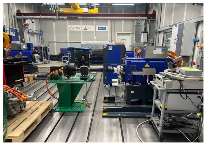
A prototype MRB system (Figure 3) was tested on a dynamometer to provide a baseline thermal verification for the numerical model. The experimental tests were conducted in an uncooled configuration (i.e., no integrated rotor/stator liquid-cooling circuit) and was used specifically to verify the heat-generation implementation adopted in the CFD model (MRF viscous dissipation during magnetic activation and coil heat input) and the imposed thermal boundary-condition strategy prior to evaluating the cooling designs numerically.

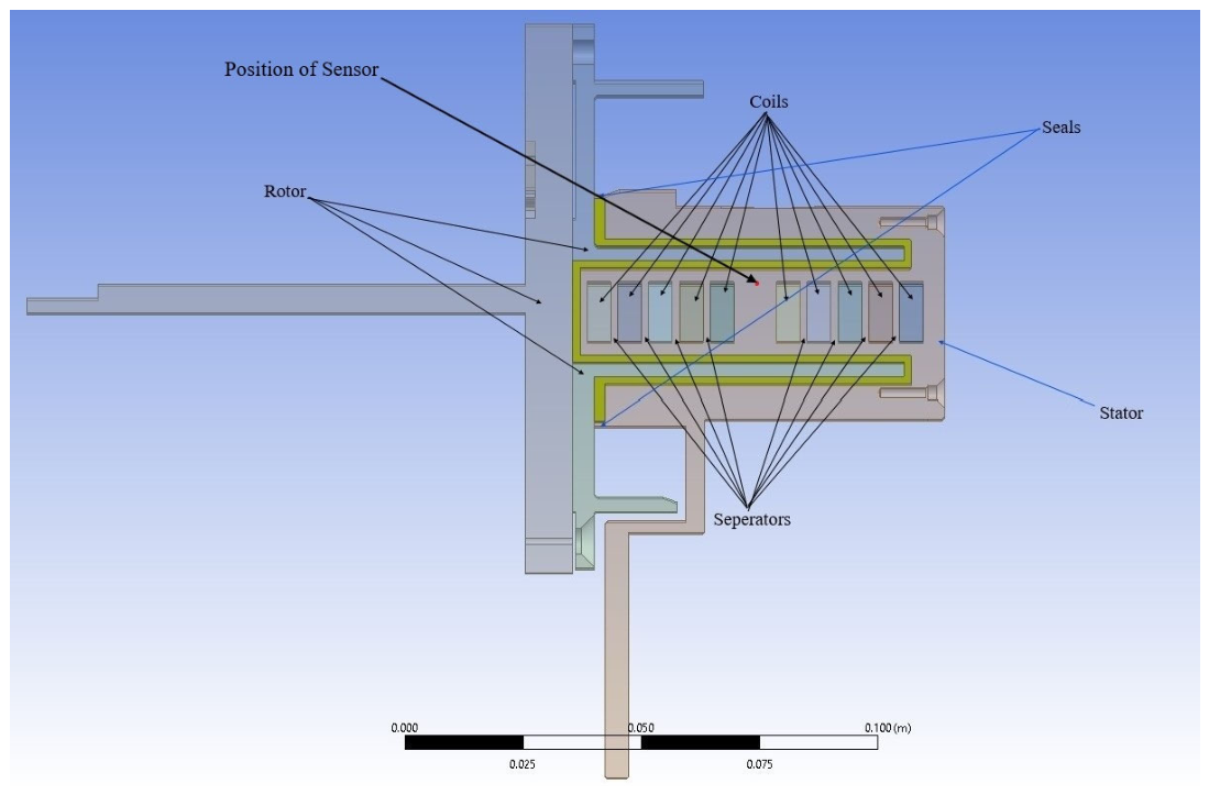
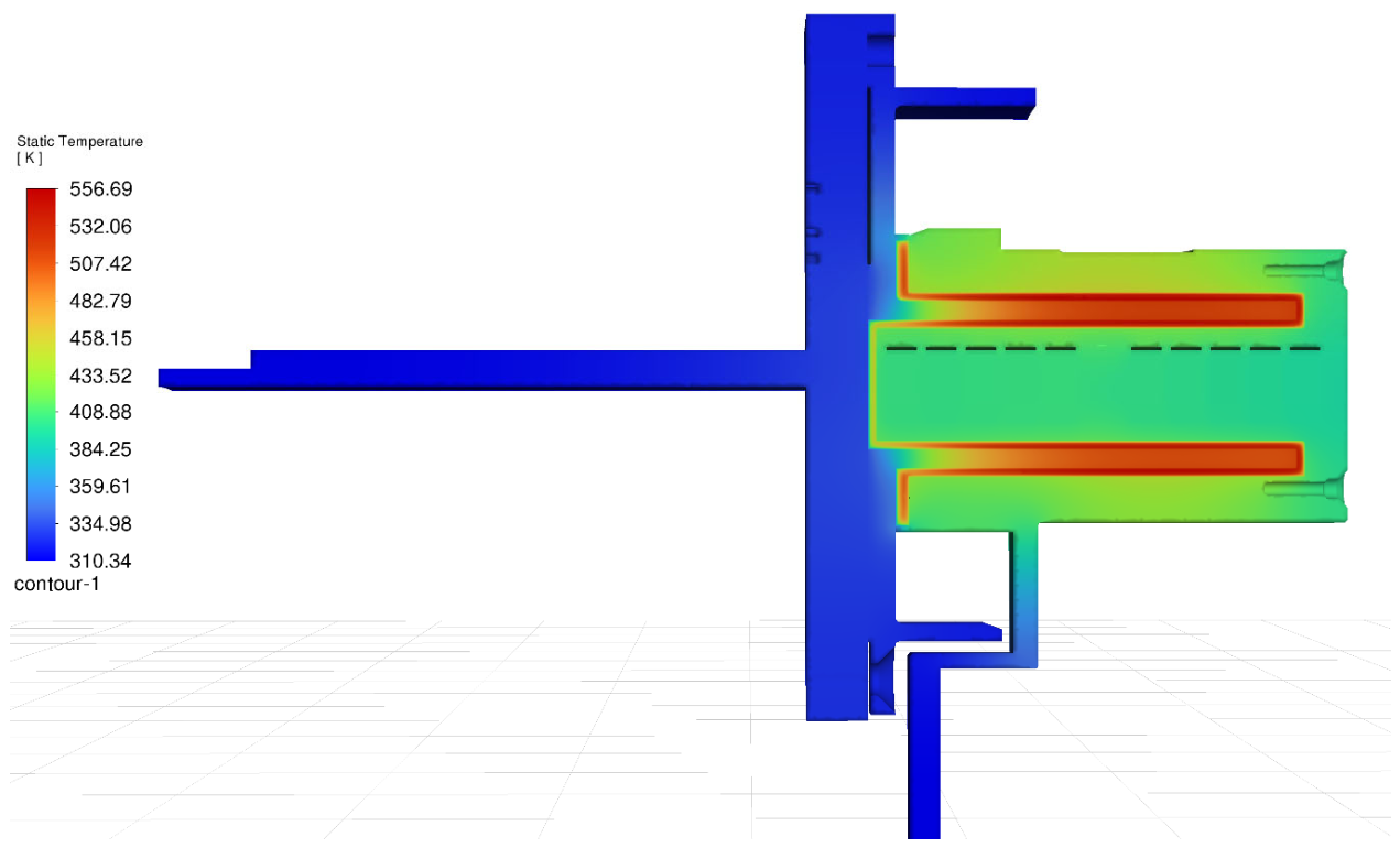
During the test, a limit braking maneuver representative of the simulated operating condition was performed, and the thermal response was monitored using a temperature sensor embedded in the MRB housing at the location shown in Figure 4. The ambient air temperature during the experiment was 25 °C, and the assembly was exposed to natural heat exchange with the surroundings.

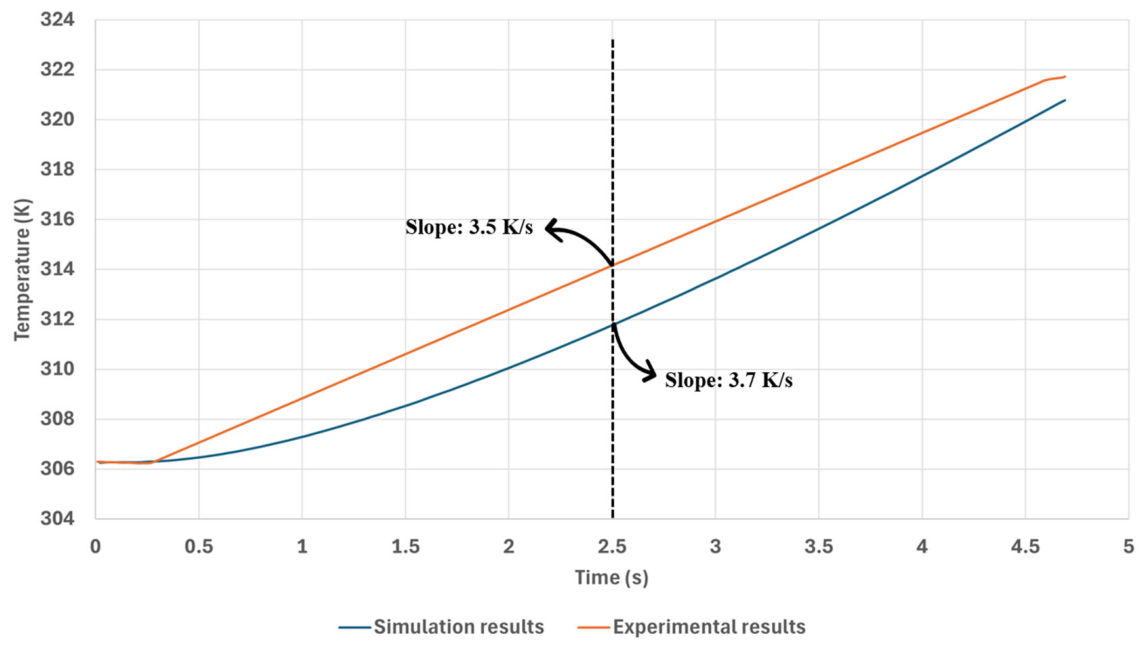
The CFD verification comparison therefore focuses on matching the measured housing temperature time history and its temperature-rise rate during the transient event (Figure 5). The simulation reproduced the overall trend and rise-rate behavior, while underpredicting the measured temperature rise by approximately 7.06%. This level of agreement supports the use of the adopted heat-generation formulation and internal boundary-condition implementation for the subsequent cooling-architecture comparisons, while recognizing that the experiment and CFD do not share identical external heat-loss conditions. It is important to note the direction of this deviation. Because the external boundaries were treated as adiabatic, the numerical model suppresses the external convective and radiative heat rejection that occurs in the physical test and would therefore be expected to overpredict, rather than underpredict, the measured temperature rise. Since the model instead underpredicts the measurement by 7.06%, the neglected external convection and radiation cannot account for this deviation; including them would lower the predicted temperature further and widen the discrepancy. The 7.06% deviation is therefore attributed to the combined uncertainties inherent in a single-sensor, single-event comparison, including local mismatch between the embedded-sensor position and the CFD extraction point, uncertainty in the effective heat generation during the dynamometer test, simplified MRF rheology, constant material properties, and simplified representation of thermal contact paths and local heat spreading. This direction is also compatible with a modest underestimation of the effective internal heat input. The conservative +20% heat-load margin applied in the subsequent cooling simulations reduces the risk that such a modest underestimate would affect the comparative cooling conclusions, although it does not replace direct experimental validation of the cooled configurations. Two factors contribute to systematic uncertainty in the baseline comparison. First, the CFD framework was developed primarily to evaluate internal heat-generation mechanisms and internal heat-transfer paths under a conservative boundary assumption for the subsequent cooling-architecture comparisons; therefore, the external surfaces were treated as adiabatic in the baseline CFD model to avoid introducing additional uncertain parameters (external natural convection coefficient, surface emissivity, and effective exposed area), which were not measured during testing. As a result, the experimental verification is interpreted as a baseline trend check of the internal heat-source implementation rather than a calibrated “as-tested” heat-loss model. Second, the experimental sensor provides temperature at a single housing location. To ensure a consistent comparison, the CFD temperature was extracted at the corresponding sensor position on the housing (point/patch monitoring at the same position shown in Figure 4, rather than relying only on volume-averaged temperatures. This approach allows a direct like-for-like comparison at the measurement point while acknowledging that a single sensor cannot capture the full spatial temperature gradients that develop across the MRF gap and the rotor/stator interfaces during the braking phase.

A fully “as-tested” external boundary condition could be imposed using a combined convection–radiation boundary at 300 K; however, this would require additional measurements or justified estimates of the external heat-transfer coefficient and surface emissivity. This is left for future work when the necessary boundary-condition characterization becomes available.

It should be emphasized that direct experimental validation is available only for the uncooled prototype configuration and from a single housing-embedded temperature sensor. The rotor-only, stator-only, and combined cooling configurations are therefore assessed numerically without a dedicated cooled prototype experimental counterpart. The reliability of the cooling-case comparison is based on the consistent use of the same heat-generation formulation, material assumptions, duty-cycle definition, and conjugate heat-transfer framework across all configurations. In this sense, the uncooled experimental comparison provides baseline support for the internal heat-generation implementation and transient thermal response before the coolant passages are introduced. In addition, the mesh, boundary-layer, and time-step independence studies reported in Table 5, Table 6 and Table 7 support the numerical robustness of the comparative results. The adiabatic external boundary condition and the +20% heat-load margin were also adopted as conservative assumptions for the thermal comparison, although they do not replace direct experimental validation of the cooled configurations. Therefore, the absolute temperature levels predicted for the cooled configurations remain subject to uncertainty, and the cooling results should be interpreted as comparative CFD predictions of the relative thermal effectiveness of the proposed architectures rather than as fully validated cooled prototype performance. On this comparative basis, the relative ranking of the configurations, combined rotor–stator cooling yielding the lowest predicted temperatures, followed by the single-side cooling configurations, with all cooled cases improving upon the uncooled baseline, is considered the most robust outcome of the study.

The adoption of an adiabatic external boundary condition merits further justification. The objective of the present study is to compare the internal liquid-cooling architectures and to assess whether internal cooling alone can manage the thermal load under repeated severe braking. The external air-side heat transfer of an in-wheel brake is strongly vehicle- and installation-dependent, being governed by wheel arch geometry, rim design, brake shielding, vehicle speed, ducting strategy, local blockage, possible forced-air paths, exposed surface area, and the radiation environment. These parameters were not characterized experimentally in the present work and would differ between vehicle platforms. Prescribing a specific external convection coefficient, air velocity, or radiation boundary would therefore make the results representative of one assumed installation rather than of the cooling architecture itself and would introduce additional uncontrolled boundary parameters. Moreover, because such an external boundary would not act identically on the rotor-only, stator-only, and combined configurations, it could partially mask the differences between cooling architectures that this study is intended to isolate. The adiabatic condition instead applies an identical external boundary to all configurations, so that the observed differences are attributable primarily to the internal liquid-cooling design. It is also conservative with respect to internal temperature accumulation, since real external heat rejection would generally reduce heat accumulation and lower the predicted temperature levels. Absolute in-vehicle temperature prediction nonetheless requires the external air-side physics to be represented explicitly; a dedicated CFD study incorporating vehicle-specific convection and radiation boundary conditions, informed by representative wheel arch airflow for a defined installation, is therefore identified as part of future work.

3. Results

3.1. Thermal Behavior Without Cooling

Figure 6 shows the uncooled baseline response over 10 duty cycles. The MRF temperature increases sharply during each deceleration (braking) phase and decreases only modestly during acceleration and constant-speed phases.

Unless otherwise stated as local spatial maxima, all reported temperature histories and convergence-table temperatures are volume-averaged over the corresponding component region, namely MRF, rotor, or stator.

After ten braking cycles, the maximum volume-averaged MRF temperature reaches 501.05 K, exceeding the 420 K operational threshold adopted in this study. This value represents the maximum over time of the volume-averaged MRF temperature; the local spatial maximum temperature is higher, as reflected in the color scale of Figure 7. To quantify the phase-wise thermal loading, the phase-resolved internal heat input was extracted using Equations (4)–(6), where the instantaneous internal heat input ${\dot{Q}}_{\mathrm{in}}\left(t\right)$ is defined as the sum of MRF viscous dissipation and coil heating during braking. For the 5° periodic sector, the phase-averaged heat-generation powers were 37 W for acceleration, 90 W for constant-speed operation, and 795 W for deceleration/braking. Because the three phases have different durations, the relative thermal contributions over a complete duty cycle are evaluated from the phase energies, $E_i=P_i\mathsf{\Delta }{t}_i$, rather than from the phase-averaged powers directly. Using the phase durations of 8.5 s, 20 s, and 2.5 s, the corresponding energy inputs in the 5° sector are 314.5 J for acceleration, 1800 J for constant-speed operation, and 1987.5 J for braking, giving a total of 4102 J per cycle. The braking phase therefore contributes approximately 48.5% of the cycle energy, the constant-speed phase approximately 43.9%, and the acceleration phase approximately 7.7%. The braking phase remains the most intense in terms of instantaneous heat-generation power and drives the sharp per-cycle temperature rises, whereas the constant-speed phase contributes comparably to the total cycle energy because of its substantially longer duration. For the full-annulus brake $(S_{\theta }=72)$, the corresponding phase-averaged thermal powers are $2.66\hspace{0.17em}\mathrm{k}\mathrm{W}$ for acceleration, $6.48\hspace{0.17em}\mathrm{k}\mathrm{W}$ for constant-speed operation, and $57.24\hspace{0.17em}\mathrm{k}\mathrm{W}$ for braking. The corresponding phase thermal energies are $22.64\hspace{0.17em}\mathrm{k}\mathrm{J}$, $129.60\hspace{0.17em}\mathrm{k}\mathrm{J}$, and $143.10\hspace{0.17em}\mathrm{k}\mathrm{J}$, respectively, giving $295.34\hspace{0.17em}\mathrm{k}\mathrm{J}$ per duty cycle. The mechanical component of these thermal inputs can be checked from $P=M\omega$. The braking-phase heat comprises the MRF gap dissipation $(777.62\hspace{0.17em}\mathrm{W}$ per sector, approximately $55.99\hspace{0.17em}\mathrm{k}\mathrm{W}$ at full annulus, and approximately $140.0\hspace{0.17em}\mathrm{k}\mathrm{J}$ over $2.5\hspace{0.17em}\mathrm{s})$, which represents the mechanical braking work, and the coil Joule heating (approximately 1.25 kW at full annulus, corresponding to $3.1\hspace{0.17em}\mathrm{k}\mathrm{J}$ over the braking phase), which is electrically supplied. The constant-speed field-OFF power of $6.48\hspace{0.17em}\mathrm{k}\mathrm{W}$ at $\omega =120\hspace{0.17em}\mathrm{r}\mathrm{a}\mathrm{d}/\mathrm{s}$ corresponds to an equivalent residual drag torque of approximately $54\hspace{0.17em}\mathrm{N}\cdot \mathrm{m}$. For the braking phase, with the imposed ramp decreasing linearly from $120\hspace{0.17em}\mathrm{r}\mathrm{a}\mathrm{d}/\mathrm{s}$ to $0\hspace{0.17em}\mathrm{r}\mathrm{a}\mathrm{d}/\mathrm{s}$, the average angular velocity is $60\hspace{0.17em}\mathrm{r}\mathrm{a}\mathrm{d}/\mathrm{s}$, and the mechanical braking power of $55.99\hspace{0.17em}\mathrm{k}\mathrm{W}$ gives a phase-equivalent braking torque of approximately $933\hspace{0.17em}\mathrm{N}\cdot \mathrm{m}$. These are energy-equivalent phase values, not instantaneous torque histories.

Figure 7 provides the temperature contour at the end of the 10-cycle sequence, and Figure 8 and Figure 9 show the rotor and stator temperature histories, respectively, over the same duty cycle.

The upper limit of the color scale corresponds to the local spatial maximum temperature, which is higher than the maximum volume-averaged MRF temperature of 501.05 K.

3.2. Cooling Case Definition and Heat Load Margin

All cooling simulations (rotor-only, stator-only, and combined cooling) were performed under a conservative heat-load condition in which the internal heat sources (MRF viscous dissipation and coil volumetric heating during braking) were scaled by +20% relative to the baseline uncooled case. The applied phase heat inputs for the 5° periodic sector are summarized in

Table 8. Heat-load margin applied in cooling simulations (5° periodic sector).

Phase	Baseline Heat Input (W)	Cooling Case Heat Input (W)
Acceleration	37	44.4
Constant speed	90	108
Deceleration	795	954
Coil heat input during braking	17.38	20.86

.

3.3. Rotor Cooling Results

Two rotor cooling-channel layouts were considered: a constant cross-section channel and a variable cross-section (tapered) channel in which the flow area changes along the passage as the radius increases. In these layouts, the quoted 5° refers to the angular aperture of an individual cooling passage, whereas the full periodic pitch additionally includes the inter-channel solid land. The variable-cross-section option accommodates 60 channels, each with a 5° aperture and a 1° inter-channel land, giving a 6° pitch $({360}^{\circ }/6^{\circ }=60)$. The constant-cross-section option accommodates 70 channels, each with a 5° aperture and an approximately 0.143° inter-channel land, giving a pitch of approximately 5.143° $({360}^{\circ }/{5.143}^{\circ }\approx 70)$. The constant-cross-section option was evaluated solely through the analytical comparison of Equations (15) and (16), and only the variable-cross-section passage concept was subsequently simulated in CFD. The very narrow inter-channel land required by the 70-channel layout also represents an additional manufacturing and structural drawback alongside its lower predicted heat-transfer potential. Using Newton’s law of cooling, the variable cross-section layout provides a substantially larger wetted area, estimated to be about five times that of the constant cross-section option. The constant cross-section option, however, yields higher coolant velocities because the flow area does not expand. Using the standard turbulent internal-flow heat-transfer scaling, for which the Nusselt number and therefore the convective heat-transfer coefficient scale approximately with ${Re}^{0.8}$, the following relation was adopted [40]:

$$h \propto V^{0.8}$$

(15)

Based on the area comparison, the constant cross-section velocity can be up to six times higher, giving $h_{\mathrm{const}}/h_{\mathrm{var}}\approx 6^{0.8}\approx 4.1$. The combined effect can be expressed through the ratio of the overall heat-transfer potential $\left(hA\right)$:

$${\displaystyle \frac{{\left(hA\right)}_{var}}{{\left(hA\right)}_{const}}}\approx {\displaystyle \frac{A_{var}}{A_{const}}}\ast {\left({\displaystyle \frac{V_{var}}{V_{const}}}\right)}^{0.8}\approx 1.2$$

(16)

Equation (16) indicates a higher overall heat-transfer potential for the variable cross-section design despite the lower local velocity; therefore, the variable cross-section rotor passage was selected for the CFD simulations (Figure 10).

Figure 11 and Figure 12 show that, during the acceleration phase, the area-weighted outlet total pressure increases with rotor angular velocity, and the outlet mass flow rate increases with rotor angular velocity. Figure 13 shows secondary-flow structures in the rotating passage.

Figure 14, Figure 15 and Figure 16 compare uncooled and rotor-only cooling cases over 10 duty cycles. Rotor-only cooling reduces MRF temperature relative to the uncooled case (Figure 14) and reduces rotor temperature (Figure 15), while stator temperatures remain relatively high (Figure 16). The MRF temperature in the rotor-only case remains close to the adopted thermal limit under the conservative heat-load condition.

3.4. Stator Cooling Results

Figure 17 shows the stator cooling passage geometry with parallel channels. Figure 18, Figure 19 and Figure 20 compare uncooled and stator-only cooling cases. Stator cooling reduces stator peak temperature by approximately 120 K relative to the uncooled case (Figure 18). The MRF temperature in the stator-only cooling case remains higher than in the rotor-cooled case (Figure 19). Rotor temperatures decrease by approximately 20 K under stator-only cooling (Figure 20).

3.5. Combined Rotor–Stator Cooling Results

Figure 21, Figure 22 and Figure 23 compare the uncooled, rotor-only, stator-only, and combined rotor–stator cooling configurations over 10 duty cycles. In the combined configuration, the MRF temperature remains below 400 K throughout the 10-cycle sequence (Figure 21), in contrast to the uncooled case, which reaches 501.05 K after ten cycles. In addition, Figure 21 shows that, after the first cycle, the MRF temperature exhibits a clear partial recovery during the acceleration phases, with reduced cycle-to-cycle accumulation relative to the single-cooling cases.

The combined configuration also yields the lowest rotor and stator temperatures among the configurations evaluated (Figure 22 and Figure 23).

4. Discussion

The uncooled results show a step-like temperature evolution that is governed not only by how much energy each phase delivers but also by how concentrated that energy is in time. Although the braking phase contributes approximately half of the cycle energy, about 48.5%, it delivers this energy in only 2.5 s at the highest instantaneous power; the resulting heat-generation rate far exceeds the rate at which the surrounding structure can dissipate heat over such a short interval, producing the sharp temperature rise seen in each cycle. By contrast, the constant-speed phase contributes a comparable share of the cycle energy, about 43.9%, but spreads it over 20 s, so its instantaneous thermal loading is milder. Because the short, intense braking pulses are followed by acceleration and constant-speed phases that provide insufficient time for the assembly to return to its initial temperature, heat accumulates progressively from cycle to cycle. The corrected energy split also shows that the constant-speed phase is a major contributor to the total cycle energy. This contribution arises from the residual field-OFF viscous drag associated with ${\mu }_{\mathrm{O}\mathrm{F}\mathrm{F}}=0.114\hspace{0.17em}\mathrm{P}\mathrm{a}\cdot \mathrm{s}$ and the present prototype geometry, corresponding to an off-state drag torque of approximately $54\hspace{0.17em}\mathrm{N}\cdot \mathrm{m}$ at full scale. This off-state drag is the expected consequence of shearing a viscous MRF-filled gap at high speed and is itself a heat source contributing to the thermal load addressed here; the present configuration should therefore not be interpreted as an optimized low-drag field-OFF design. Reducing off-state drag is a necessary future design objective before vehicle-level implementation and may require a lower field-OFF-viscosity MRF, optimization of the gap and wetted shear area, minimization of residual magnetic-field effects, and, where required, mechanical or hydraulic decoupling during non-braking operation. The gradual increase in rotor and stator temperatures indicates progressive thermal storage in solid components, which reduces the effective temperature gradient available for heat rejection from the MRF gap over successive cycles.

The rotor-only case demonstrates that rotation influences the coolant pressure field and flow rate (Figure 11 and Figure 12). However, rotor cooling alone does not fully suppress MRF heating because the stator-side temperature remains elevated (Figure 16), reducing the rotor–MRF–stator temperature gradient and limiting the net heat flux that can be extracted from the gap during non-braking phases. In other words, rotor cooling strengthens one heat-removal path but does not address the stator-side thermal resistance.

Stator-only cooling substantially reduces stator temperature (≈120 °C reduction), but rotor temperature decreases only modestly (≈20 °C). This implies that a large fraction of the heat generated in the gap still accumulates in the rotating structure and must be conducted through the rotor before it can be rejected. A contributing factor is the asymmetry in thermal inertia and heat spreading between rotor and stator: the stator typically has larger surface area and higher thermal mass, so when the rotor is actively cooled the stator can still act as a comparatively effective passive sink; when only the stator is cooled, the rotor—having lower mass and smaller heat-spreading area—can heat up rapidly and elevate MRF temperature even if the stator remains cooler.

The combined configuration reduces cumulative heating because it strengthens heat rejection on both sides of the MRF gap. By lowering both rotor and stator temperatures (Figure 22 and Figure 23), the combined layout preserves a larger effective temperature gradient away from the gap during the full duty cycle. As a result, heat removal during the non-braking phases becomes comparable to a significant portion of the prior braking heat input, which is reflected in the partial temperature recovery during acceleration phases observed in Figure 21. The response does not represent a strict steady state—because braking continues to repeat—but it trends toward a quasi-periodic (cyclic) thermal regime, where the temperature trajectories become increasingly repeatable from cycle to cycle with limited drift.

The present study focuses on the thermal comparison of the cooling architectures and does not include a full hydraulic characterization of the coolant circuits. Pressure-drop maps, pump operating-point selection, and the corresponding parasitic energy consumption were therefore not quantified for the individual configurations; these require a complete coolant-loop definition and belong to the subsequent detailed-design stage following the thermal down-selection performed here. For such an assessment, the hydraulic pump power can be estimated from:

$$P_{hyd}=∆P\dot{V}$$

(17)

and the corresponding electrical pump power from:

$$P_{el}={\displaystyle \frac{P_{hyd}}{{\eta }_{\mathrm{p}\mathrm{u}\mathrm{m}\mathrm{p}}}}$$

(18)

where $\mathsf{\Delta }p$ is the coolant-circuit pressure drop, $\dot{V}$ is the volumetric flow rate, and ${\eta }_{\mathrm{p}\mathrm{u}\mathrm{m}\mathrm{p}}$ is the pump efficiency. Quantifying these terms for each configuration is part of the subsequent design stage. One component of the parasitic-energy question is nevertheless addressed for the rotor side: as shown in Figure 11 and Figure 12, the outlet total pressure and outlet mass flow rate of the rotor passage increase with rotor angular velocity, indicating a centrifugal self-pumping effect and suggesting a potential reduction in external pump demand during high-speed operation. This result should be interpreted as a qualitative mechanism rather than as a full pump-sizing result. With respect to manufacturability, the configurations differ in integration complexity: stator cooling is the simpler case, with channels in a stationary component, whereas integrating channels within the rotating component is more demanding—feasible but non-trivial—requiring internal passage fabrication, rotating coolant transfer through seals and manifolds, and attention to packaging, balancing, leakage control, and serviceability. The combined configuration, which yields the lowest predicted temperatures in the present CFD comparison, therefore also carries the highest integration complexity. A quantitative assessment of the complete coolant-loop hydraulic losses, pump power, and manufacturing trade-offs was outside the thermal-screening scope of this work and is identified as part of the subsequent detailed-design stage.

At the vehicle level, the MRF brake is intended to operate in coordination with regenerative braking provided by the in-wheel electric machine. The MRF brake itself is a dissipative device: it converts mechanical braking work into heat within the MRF gap and does not directly recover electrical energy; regeneration is provided by the traction machine. The electrical energy recovered during regenerative braking could, however, be used to supply auxiliary cooling components such as the coolant pump, fan, and control electronics, thereby reducing the net energy penalty of the thermal-management system. Such coordination can reduce reliance on conventional friction braking across many operating conditions, although complete elimination of friction braking, particularly at very low vehicle speed and under fail-safe and regulatory braking requirements, would require a dedicated vehicle-level safety and redundancy assessment beyond the scope of the present thermal study.

The thermal robustness of the electromagnetic excitation subsystem also requires further assessment. In the present architecture, the electromagnetic cores/coils are integrated within the stator region rather than being rotor-mounted windings. The present CFD model includes the coil/core region thermally and represents the coil heat input as a prescribed volumetric heat source; therefore, the resulting coil/core temperature field can be assessed from the thermal solution. However, the model does not include coupled electromagnetic–thermal feedback, temperature-dependent winding resistance, insulation-aging behavior, or short-circuit failure analysis. Elevated coil/core temperature may increase electrical resistance and Joule losses and may affect insulation reliability if material limits are exceeded. These effects should therefore be included in future electrothermal design work. Phase-change materials, already noted as a transient heat-buffering strategy [29], could also be investigated as a supplementary passive thermal-buffering strategy near the coils/cores, especially for short-duration heat peaks; their suitability would depend on melting temperature, latent heat capacity, thermal-conductivity enhancement, packaging volume, mass, and the ability to reject the stored heat between repeated braking events.

5. Conclusions

This paper evaluated rotor-only, stator-only, and combined rotor–stator liquid-cooling configurations for a magnetorheological-fluid brake using transient 3-D conjugate heat-transfer CFD under a repeated braking duty cycle. A baseline uncooled test was used to verify the numerical heat-generation/boundary-condition implementation prior to comparing the cooling configurations.

The main conclusions are:

• Uncooled baseline: repeated braking produces cumulative thermal storage in the assembly and drives the maximum volume-averaged MRF temperature to approximately 501 K after ten cycles, motivating active thermal management.
• Rotor-only cooling: rotor channel cooling reduces MRF and rotor temperatures compared with the uncooled case and shows a rotation-induced contribution to coolant pressurization; however, rotor-only cooling remains limited by the stator-side heat path and cannot fully suppress cumulative MRF heating over repeated cycles.
• Stator-only cooling: parallel stator channels reduce stator temperature substantially, but rotor temperatures decrease only modestly; consequently, MRF temperature remains higher than in the rotor-cooled configuration because rotor-side thermal storage and conduction become the limiting mechanism.
• Combined rotor–stator cooling: integrating both cooling circuits provides the strongest and most stable thermal response, maintaining MRF temperature below 400 K after ten cycles under a conservative +20% heat-load margin, while also yielding the lowest rotor and stator temperatures among the configurations studied.

While the integrated rotor–stator cooling concept provides the best thermal performance in the present study, it also introduces additional hardware complexity (e.g., rotating seals/manifolds, packaging constraints, and leakage/fouling risks).

Future steps should therefore focus, as a priority, on direct experimental validation of the cooled configurations using a cooled prototype and multi-point thermal instrumentation under representative vehicle conditions. This would overcome the present limitation of relying on a single-sensor, uncooled-only experimental comparison. Further work should also include system-level assessment of the complete coolant loop, including external heat losses, hardware pressure drops, and pump power, to quantify when centrifugal assistance can reduce pump demand. In parallel, design-for-manufacture improvements should be investigated to simplify the cooling architecture, for example by reducing the number of interfaces and seals and improving serviceability, while preserving the thermal benefit. In parallel, alternative or hybrid cooling concepts could be evaluated, such as vapor chambers for enhanced in-plane heat spreading and air-side rotor cooling (ducted or fin-assisted) to reduce plumbing and sealing requirements on the rotating component. Future simulations should assess sensitivity to anisotropic, field-dependent thermal conductivity in the MRF (as may occur under particle chain formation) to quantify how direction-dependent heat transport could shift local hot spots and influence the relative ranking of cooling architectures.