Figure 1.
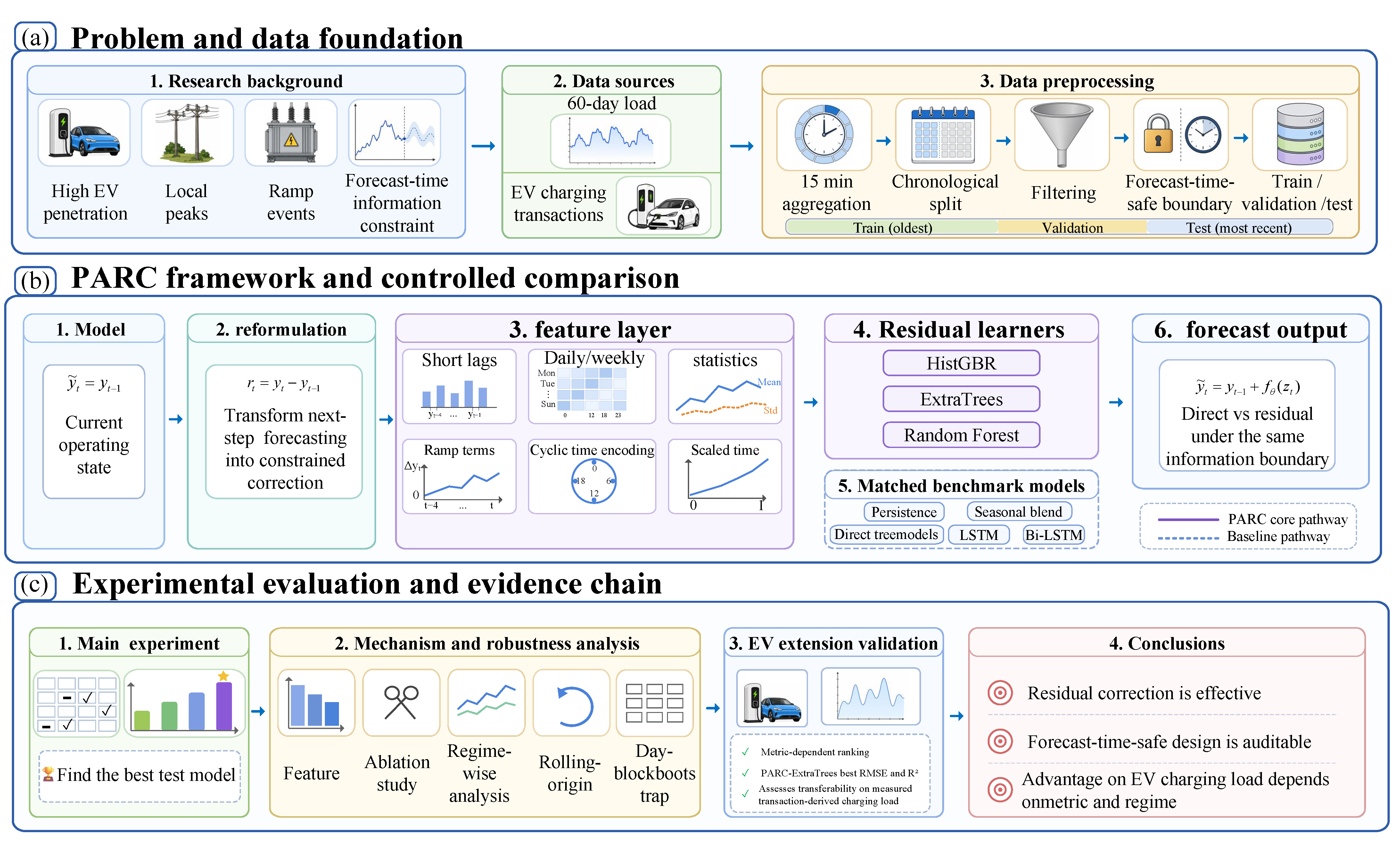
Technical route of this study. The workflow contains (a) problem and data foundation, (b) the PARC framework and controlled comparison, and (c) experimental evaluation and evidence chain.
Figure 1.
Technical route of this study. The workflow contains (a) problem and data foundation, (b) the PARC framework and controlled comparison, and (c) experimental evaluation and evidence chain.
Figure 2.
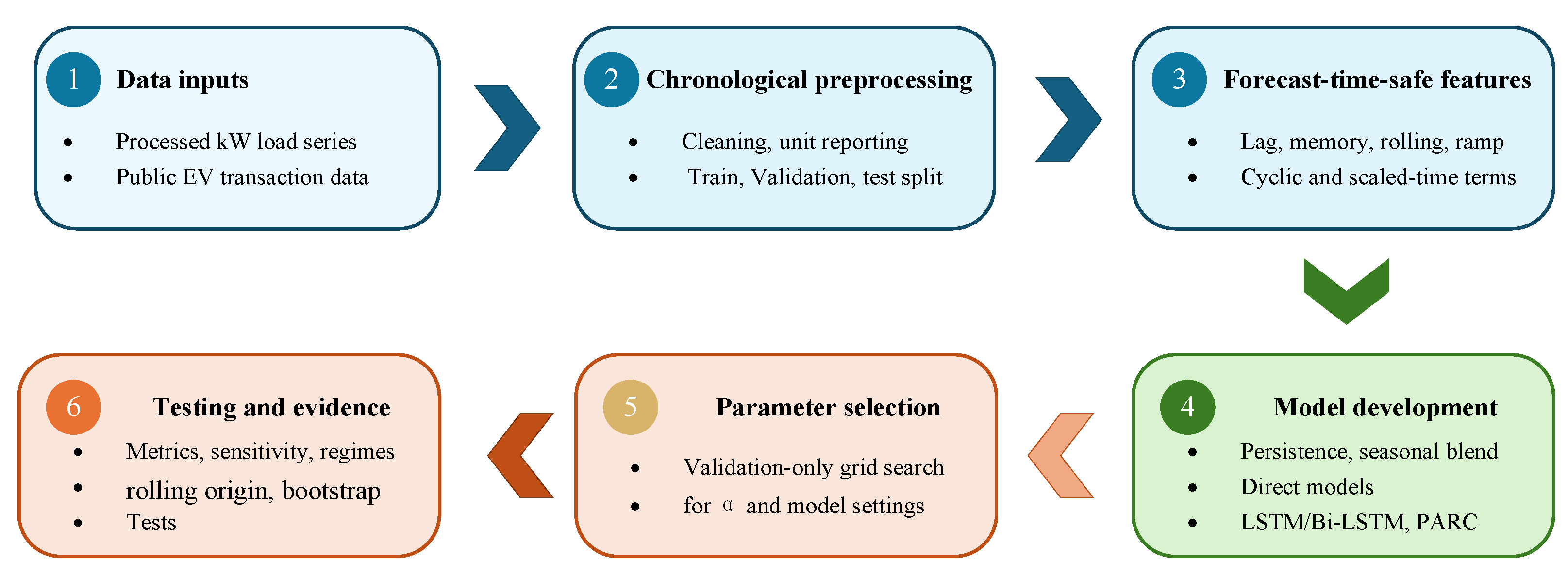
Implementation workflow used in the revised methodology section. The diagram separates validation-only parameter selection from final testing and supporting evidence checks.
Figure 2.
Implementation workflow used in the revised methodology section. The diagram separates validation-only parameter selection from final testing and supporting evidence checks.
Figure 3.
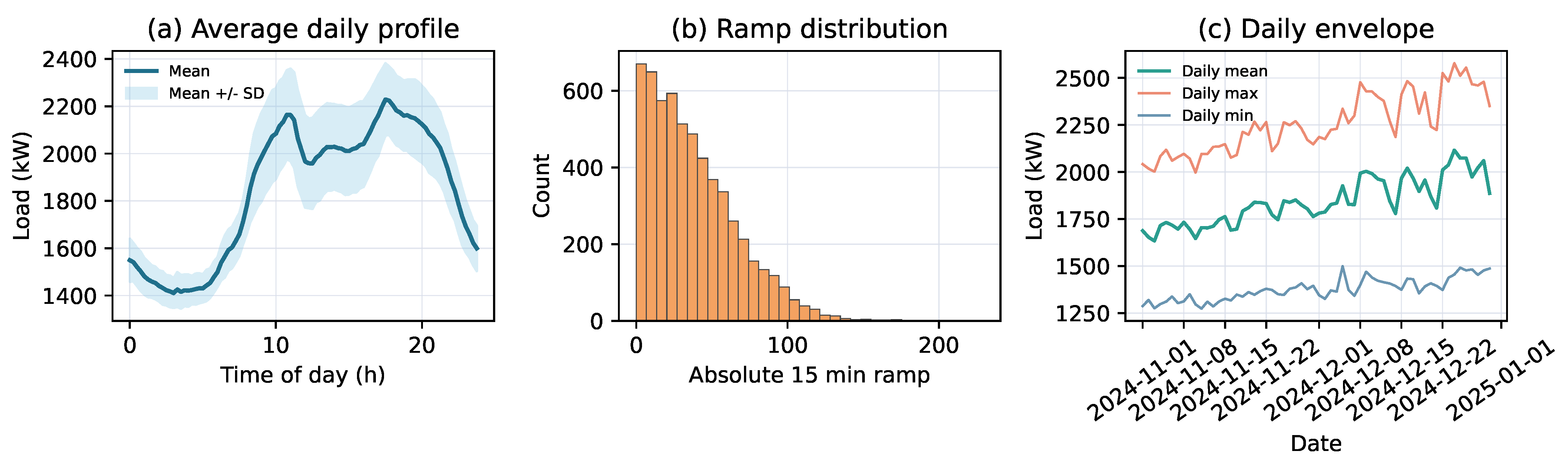
Statistical characterization of the processed distribution load proxy series. (a) Average daily profile with one-standard-deviation band; (b) distribution of absolute 15 min ramps; (c) daily minimum, mean, and maximum load envelope in kW.
Figure 3.
Statistical characterization of the processed distribution load proxy series. (a) Average daily profile with one-standard-deviation band; (b) distribution of absolute 15 min ramps; (c) daily minimum, mean, and maximum load envelope in kW.
Figure 4.
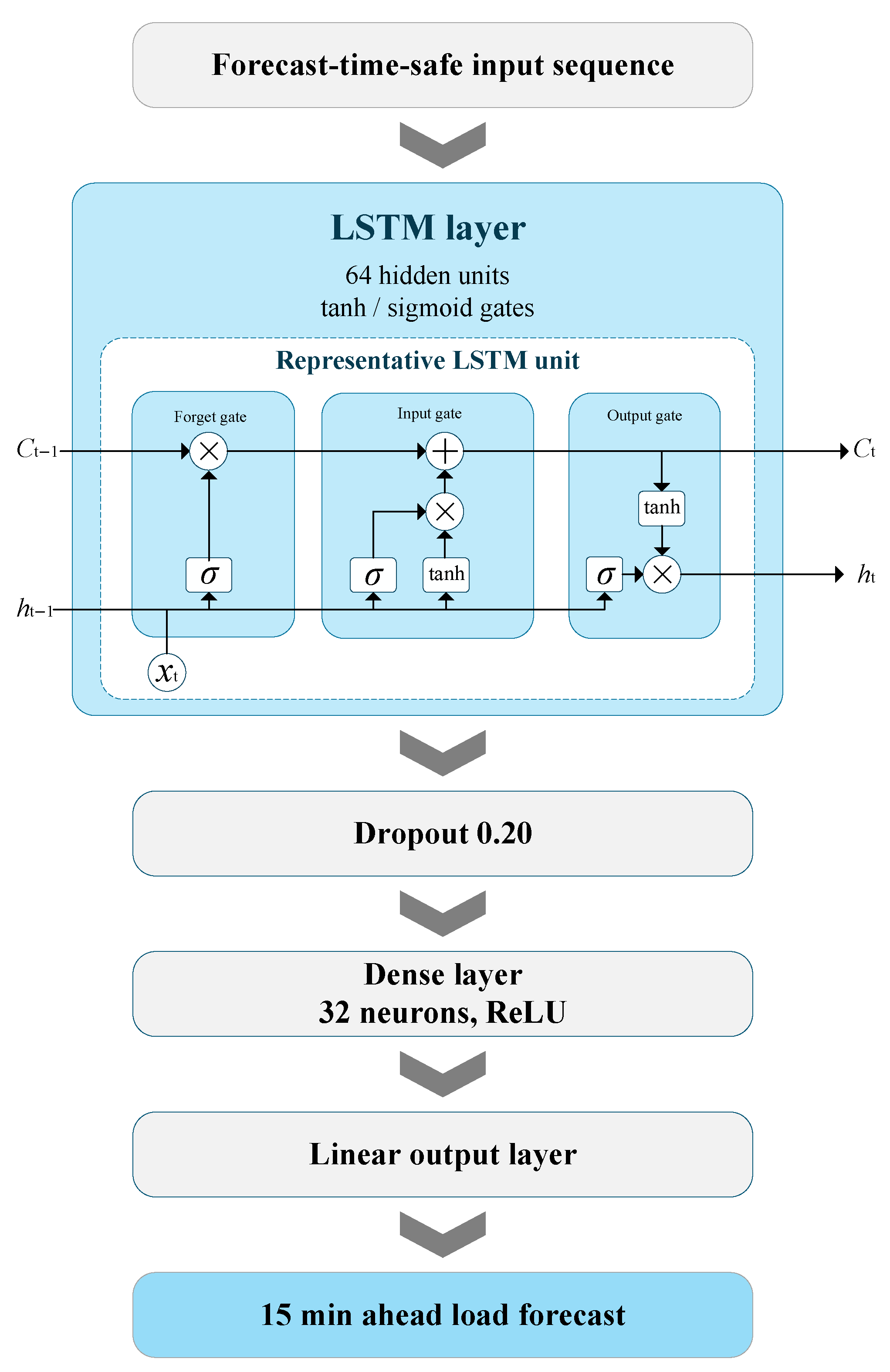
LSTM benchmark architecture used for the recurrent network comparison.
Figure 4.
LSTM benchmark architecture used for the recurrent network comparison.
Figure 5.
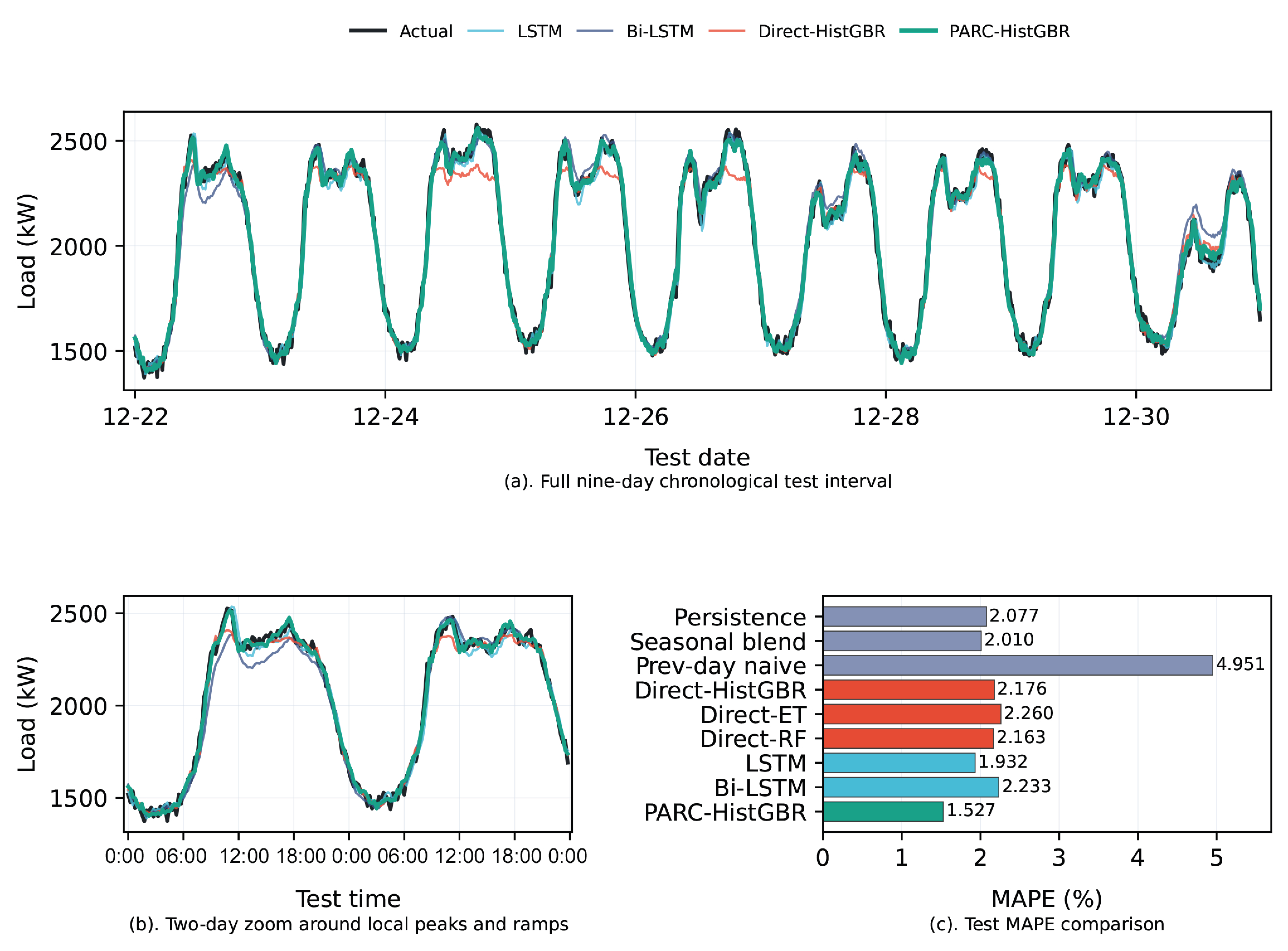
Main performance summary. (a) Full nine-day chronological test interval; (b) two-day zoom around local peaks and ramps; (c) test MAPE comparison across simple baselines, direct tree learners, recurrent networks, and PARC.
Figure 5.
Main performance summary. (a) Full nine-day chronological test interval; (b) two-day zoom around local peaks and ramps; (c) test MAPE comparison across simple baselines, direct tree learners, recurrent networks, and PARC.
Figure 6.
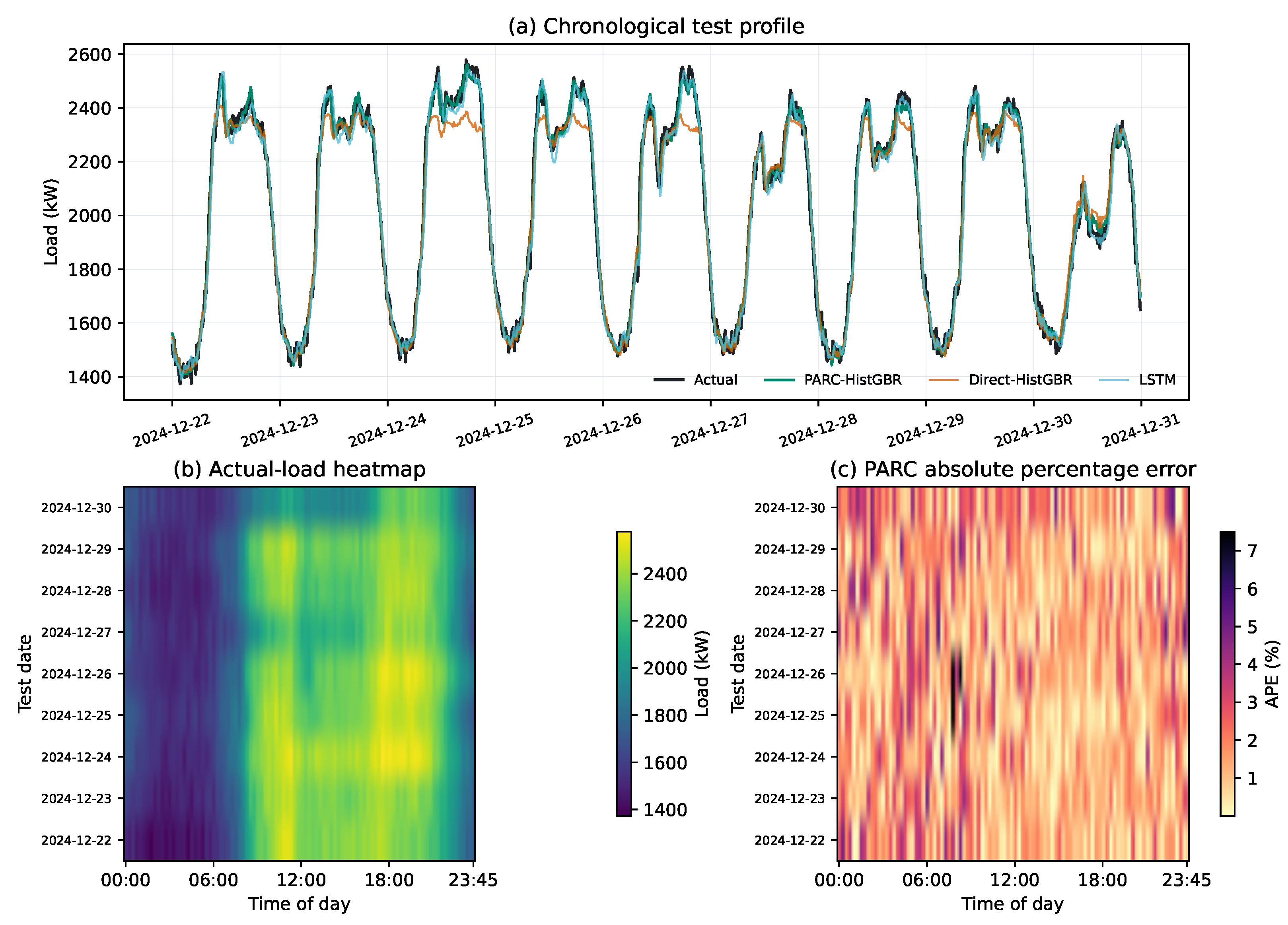
Chronological and diagnostic visualization of the nine-day test interval. (a) Actual load in kW, PARC-HistGBR, Direct-HistGBR, and LSTM forecasts over reconstructed timestamps; (b) actual-load heatmap by test date and time of day; (c) PARC-HistGBR absolute percentage-error heatmap.
Figure 6.
Chronological and diagnostic visualization of the nine-day test interval. (a) Actual load in kW, PARC-HistGBR, Direct-HistGBR, and LSTM forecasts over reconstructed timestamps; (b) actual-load heatmap by test date and time of day; (c) PARC-HistGBR absolute percentage-error heatmap.
Figure 7.
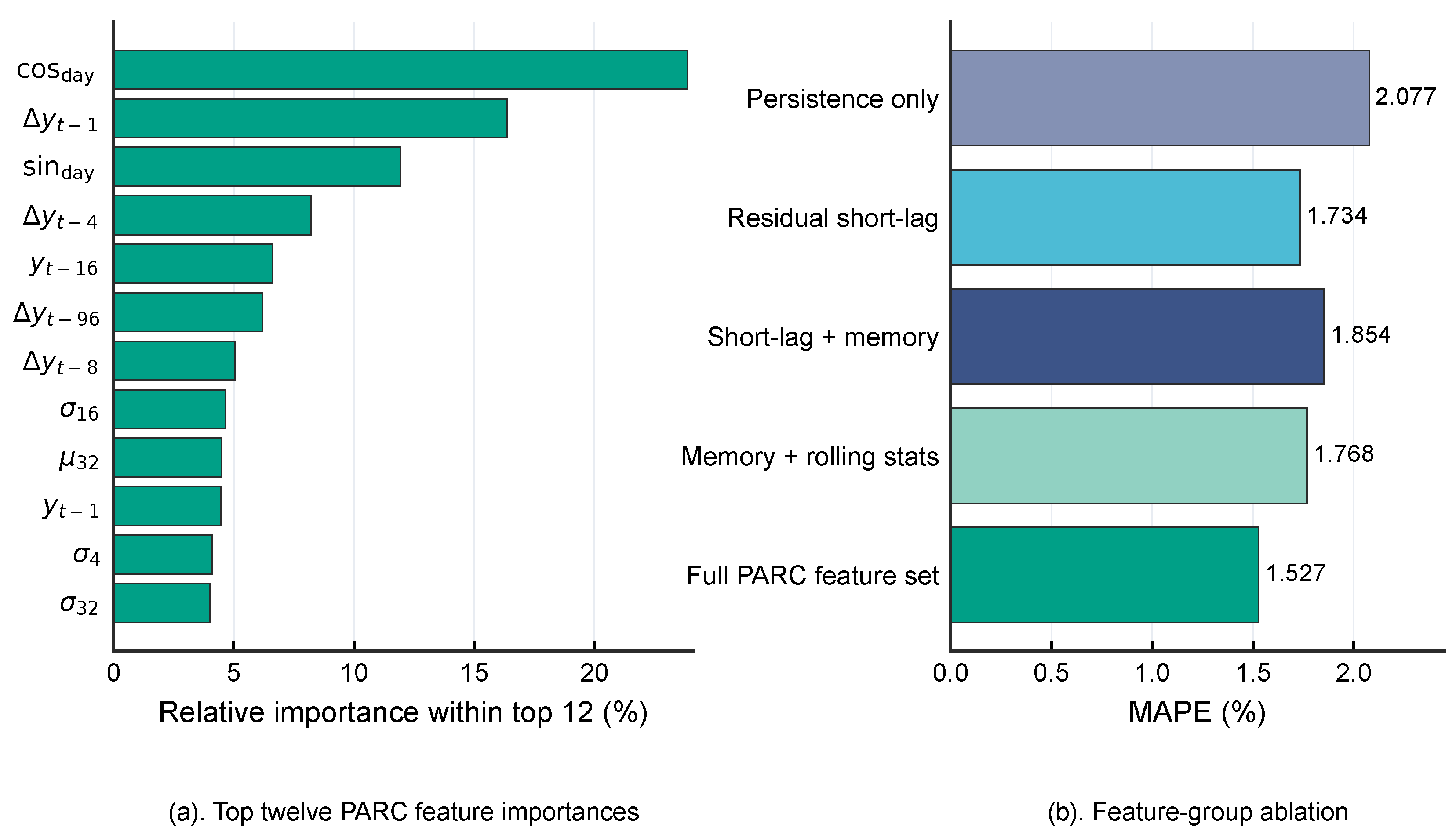
Feature mechanism summary. (a) Top twelve PARC feature importances from the ExtraTrees residual learner; (b) feature-group ablation, showing the incremental value of the full forecast-time-safe feature set.
Figure 7.
Feature mechanism summary. (a) Top twelve PARC feature importances from the ExtraTrees residual learner; (b) feature-group ablation, showing the incremental value of the full forecast-time-safe feature set.
Figure 8.
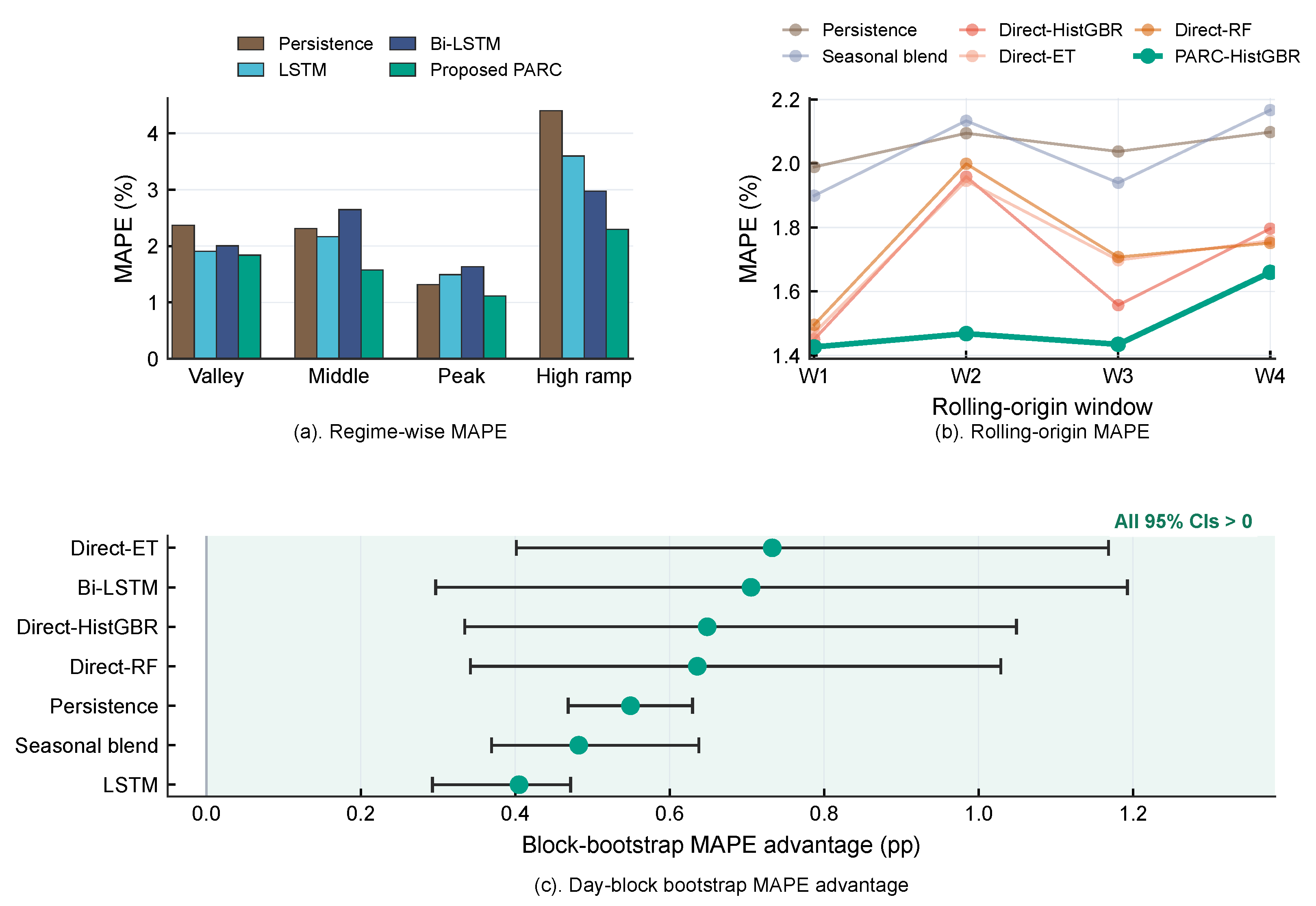
Robustness summary. (a) Regime-wise MAPE for representative models; (b) rolling-origin MAPE across four three-day windows; (c) day-block bootstrap MAPE advantage of PARC-HistGBR relative to the selected comparators shown, where positive values indicate lower MAPE for PARC-HistGBR.
Figure 8.
Robustness summary. (a) Regime-wise MAPE for representative models; (b) rolling-origin MAPE across four three-day windows; (c) day-block bootstrap MAPE advantage of PARC-HistGBR relative to the selected comparators shown, where positive values indicate lower MAPE for PARC-HistGBR.
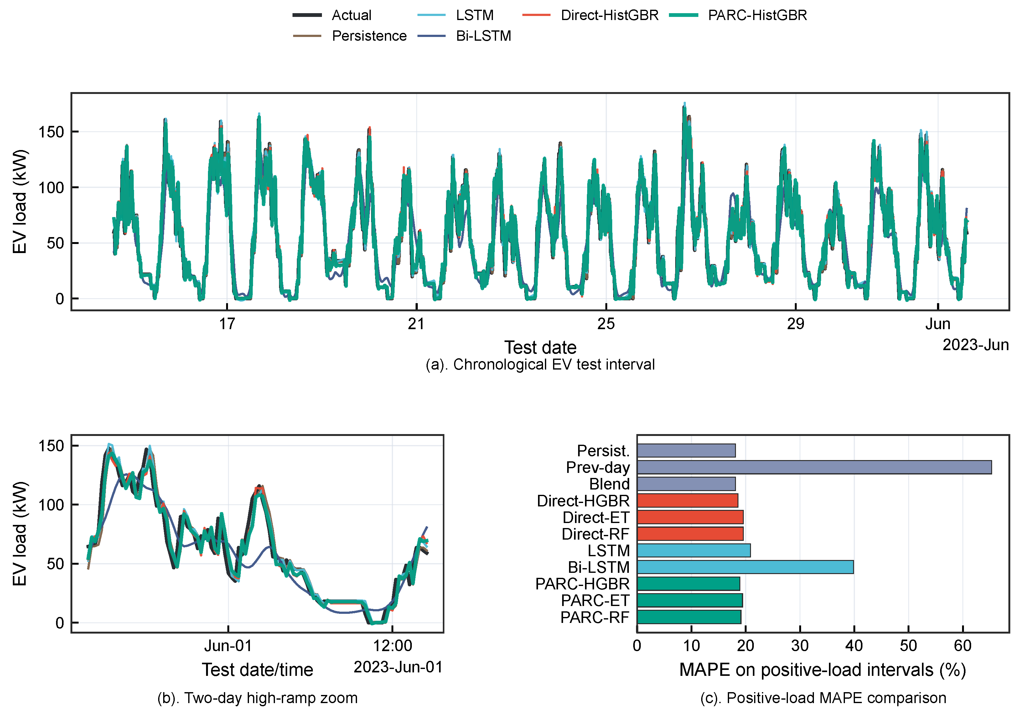
Figure 9.
Public EV charging data validation summary. (a) Chronological EV test interval; (b) two-day high-ramp zoom; (c) positive-load MAPE comparison for persistence, recurrent, direct model, and PARC variants.
Figure 9.
Public EV charging data validation summary. (a) Chronological EV test interval; (b) two-day high-ramp zoom; (c) positive-load MAPE comparison for persistence, recurrent, direct model, and PARC variants.
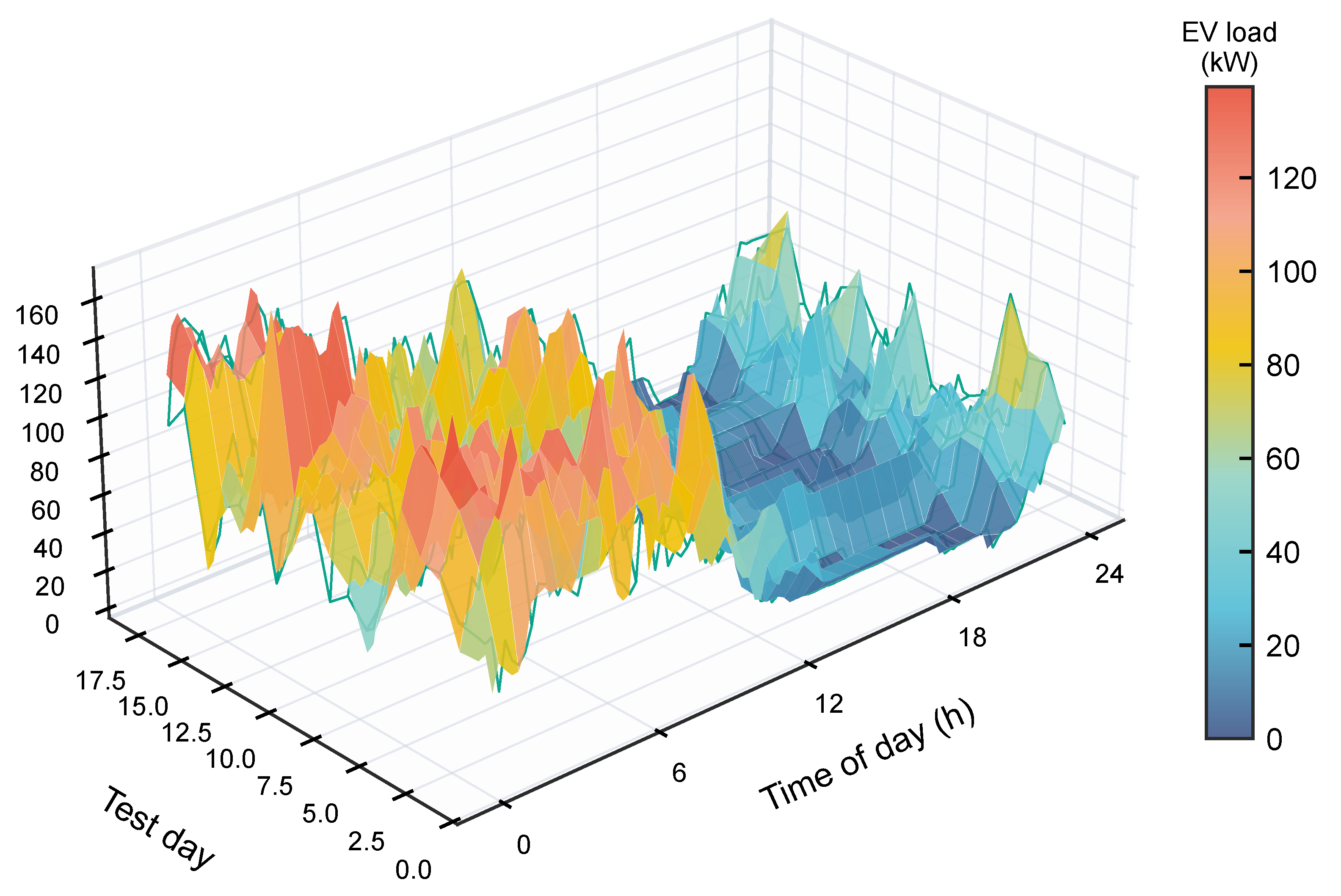
Figure 10.
Three-dimensional daily-profile visualization for the public EV charging extension. The measured transaction-derived EV load is shown as a daily surface, and the PARC-HistGBR forecast is overlaid as a green wireframe. The figure highlights the intermittency and sharp daytime charging peaks that distinguish the EV extension from the smoother distribution load proxy.
Figure 10.
Three-dimensional daily-profile visualization for the public EV charging extension. The measured transaction-derived EV load is shown as a daily surface, and the PARC-HistGBR forecast is overlaid as a green wireframe. The figure highlights the intermittency and sharp daytime charging peaks that distinguish the EV extension from the smoother distribution load proxy.
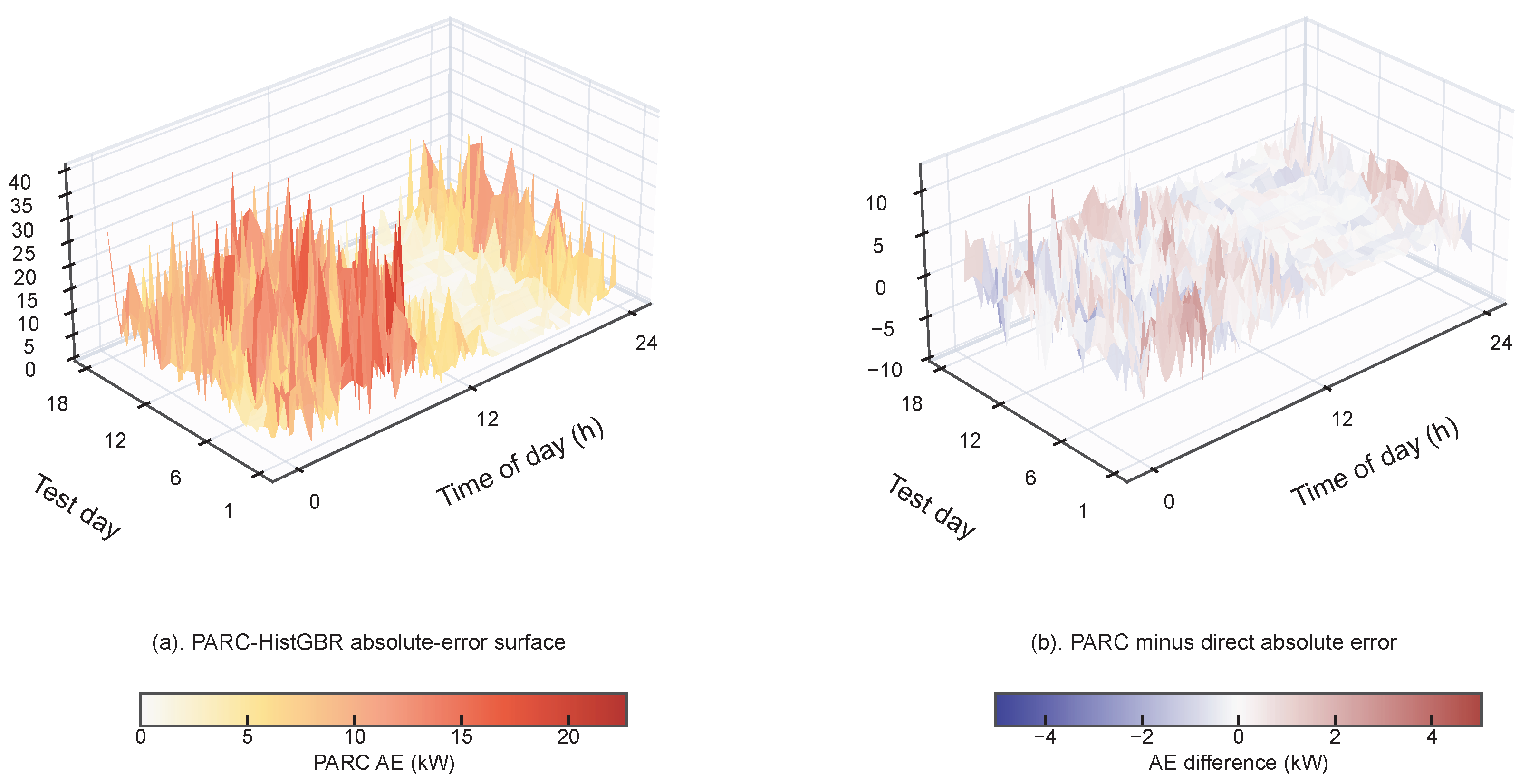
Figure 11.
Three-dimensional EV error diagnostics. (a) PARC-HistGBR absolute error surface in kW; (b) difference between PARC-HistGBR and Direct-HistGBR absolute error surfaces. Positive values indicate intervals where PARC-HistGBR has larger absolute error than the matched direct HistGBR model, and negative values indicate intervals where PARC-HistGBR has smaller absolute error.
Figure 11.
Three-dimensional EV error diagnostics. (a) PARC-HistGBR absolute error surface in kW; (b) difference between PARC-HistGBR and Direct-HistGBR absolute error surfaces. Positive values indicate intervals where PARC-HistGBR has larger absolute error than the matched direct HistGBR model, and negative values indicate intervals where PARC-HistGBR has smaller absolute error.
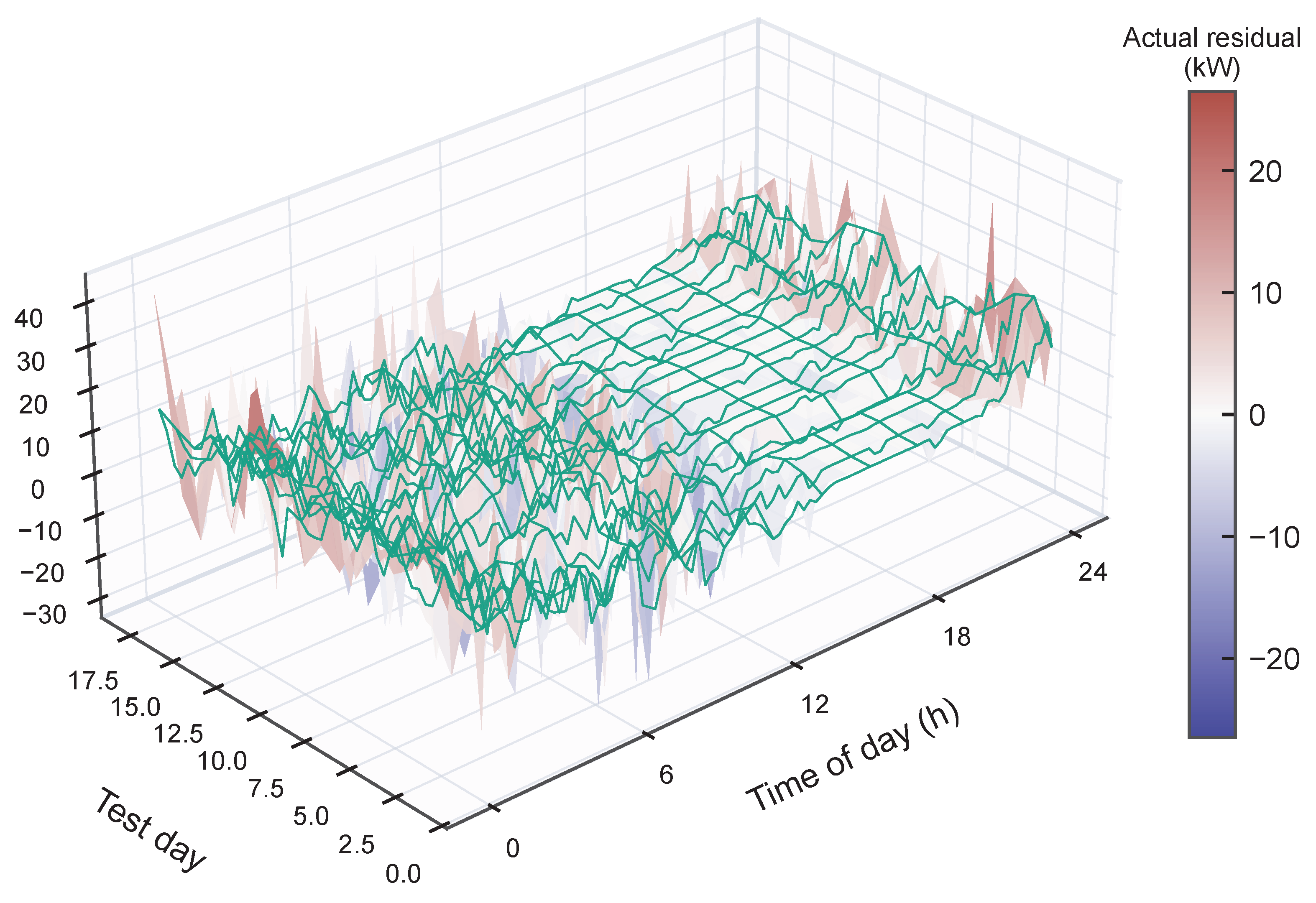
Figure 12.
Three-dimensional residual correction diagnostic for the public EV charging extension. The surface shows the actual persistence residual, and the green wireframe shows the learned PARC-HistGBR correction. The comparison makes the residual target formulation visually inspectable and explains how PARC adjusts the persistence baseline on measured EV charging data.
Figure 12.
Three-dimensional residual correction diagnostic for the public EV charging extension. The surface shows the actual persistence residual, and the green wireframe shows the learned PARC-HistGBR correction. The comparison makes the residual target formulation visually inspectable and explains how PARC adjusts the persistence baseline on measured EV charging data.
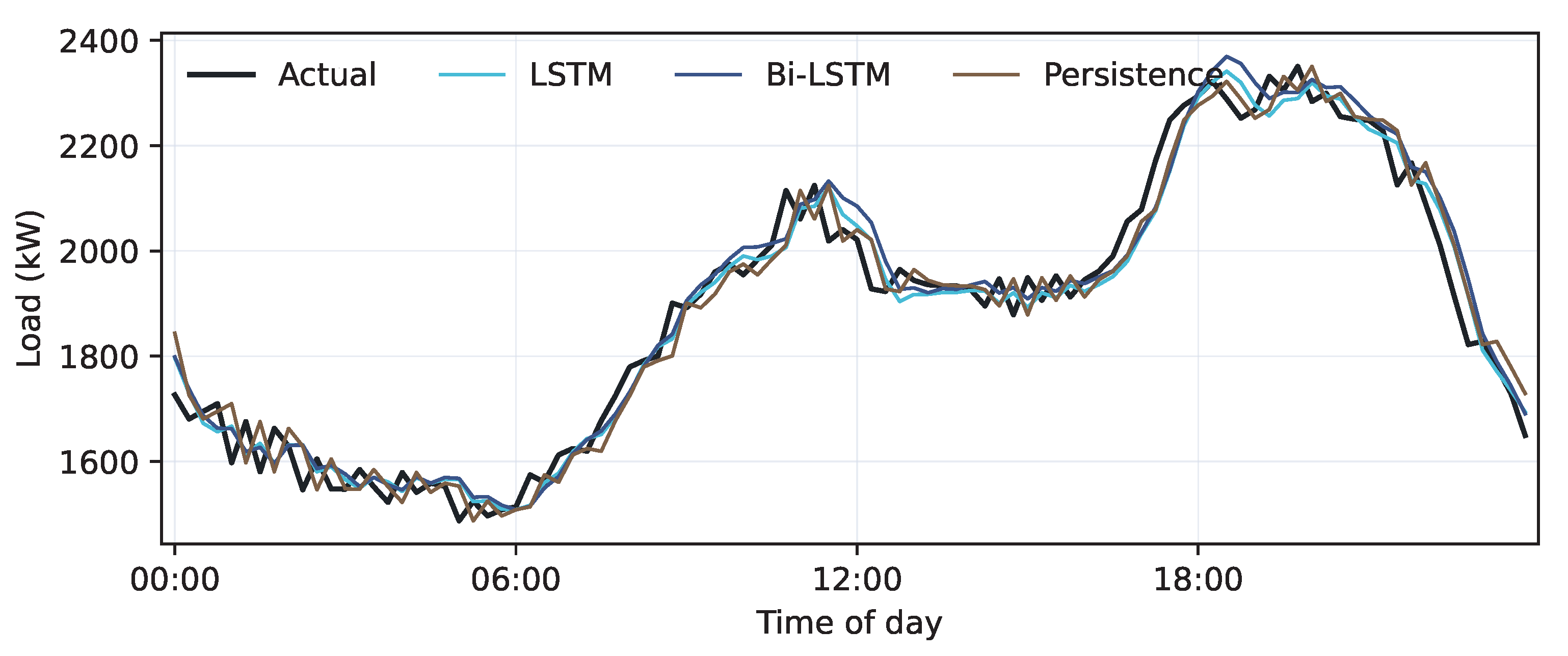
Figure 13.
Last-day forecasts using the 8-step lookback setting.
Figure 13.
Last-day forecasts using the 8-step lookback setting.
Table 1.
Research positioning of the compared method groups.
Table 1.
Research positioning of the compared method groups.
| Method Group | Benchmark Role | Interpretation for PARC |
|---|
| Persistence | Current-level anchor | Tests whether a learned correction improves the one-step baseline. |
| Previous-day-naive | Daily cycle baseline | Tests whether daily repetition alone is sufficient. |
| Direct tree controls | Same features, direct target | Separates the residual target from the tree learner and feature set. |
| LSTM and Bi-LSTM | Recurrent benchmarks | Checks PARC against nonlinear sequence models under the same data split. |
| PARC | Residual correction framework | Learns a forecast-time-safe correction to persistence. |
Table 2.
Statistical characterization of the 60-day processed distribution load proxy series.
Table 2.
Statistical characterization of the 60-day processed distribution load proxy series.
| Descriptor | Value | Descriptor | Value |
|---|
| Sampling and length | 15 min; 5760 samples (60 days) | Reported unit | kW |
Minimum/mean/
maximum load | 1274.202/1843.122/
2578.047 kW | Load factor/peak-to-average ratio | 0.715/1.399 |
Mean/95th percentile/
maximum 15 min ramp | 37.792/92.547/229.324 kW | Weekday/weekend average load | 1857.970/
1808.478 kW |
Low-load samples below
10% of peak | 0 samples | Average daily valley/peak time | 03:00/17:30 |
Table 3.
Recurrent network benchmark configuration.
Table 3.
Recurrent network benchmark configuration.
| Item | LSTM Setting | Bi-LSTM Setting |
|---|
| Input | 96 load steps (1 day); calendar only in sensitivity check | 96 load steps (1 day) |
| Architecture | LSTM(64) + dropout 0.20 + FC(32, ReLU) + linear; dense L2 | Bi-LSTM(96) + dropout 0.10 + FC/regression output |
| Optimizer/LR | Adam, , batch 32 | Adam mini-batch; 0.001; 0.30 drop after 45 epochs |
| Training | 200 epochs max; early stop 20; restore best validation weights | 90 epochs max; validation monitored; gradient threshold 1 |
| Seed/split | Seed 2026; chronological split; no random test sampling | Same protocol |
Table 4.
Worked example of one PARC-HistGBR 15 min ahead forecast.
Table 4.
Worked example of one PARC-HistGBR 15 min ahead forecast.
| Quantity | Value | Quantity | Value |
|---|
| Forecast timestamp/target index | 26 December 2024 08:15/5314 | Previous load | 1906.144 kW |
| Same-time memory / | 2004.653/1992.839 kW | 1 h rolling mean/std. | 1811.782/56.657 kW |
| Recent ramp | 150.270 kW | Daily phase sine/cosine | 0.831/−0.556 |
| Predicted residual | 74.707 kW | Final forecast | 1980.851 kW |
| Observed value/absolute error | 2135.468/154.617 kW | Absolute percentage error | 7.240% |
Table 5.
Forecast accuracy in the nine-day chronological test interval of the processed kW load series.
Table 5.
Forecast accuracy in the nine-day chronological test interval of the processed kW load series.
| Model | MAE (kW) | RMSE (kW) | MAPE (%) | |
|---|
| Persistence | 40.436 | 51.416 | 2.077 | 0.9798 |
| Seasonal blend | 39.320 | 50.089 | 2.010 | 0.9808 |
| Previous-day-naive | 101.219 | 143.435 | 4.951 | 0.8429 |
| Direct-HistGBR | 45.308 | 61.159 | 2.176 | 0.9714 |
| Direct-ExtraTrees | 47.295 | 62.433 | 2.260 | 0.9702 |
| Direct-RandomForest | 44.848 | 59.236 | 2.163 | 0.9732 |
| LSTM | 38.648 | 50.101 | 1.932 | 0.9808 |
| Bi-LSTM | 44.614 | 58.338 | 2.233 | 0.9740 |
| PARC-HistGBR | 29.865 | 37.051 | 1.527 | 0.9895 |
Table 6.
Validation and test the performance of direct and residual tree variants.
Table 6.
Validation and test the performance of direct and residual tree variants.
| Model | Validation MAPE (%) | Test MAPE (%) | Test RMSE (kW) | Test |
|---|
| Direct-HistGBR | 1.617 | 2.176 | 61.159 | 0.9714 |
| Direct-ExtraTrees | 1.624 | 2.260 | 62.433 | 0.9702 |
| Direct-RandomForest | 1.689 | 2.163 | 59.236 | 0.9732 |
| PARC-HistGBR | 1.466 | 1.527 | 37.051 | 0.9895 |
| PARC-ExtraTrees | 1.426 | 1.544 | 37.222 | 0.9894 |
| PARC-RandomForest | 1.452 | 1.544 | 37.535 | 0.9892 |
Table 7.
Additional machine learning and statistical baselines with matched PARC residual variants on the processed kW load test interval.
Table 7.
Additional machine learning and statistical baselines with matched PARC residual variants on the processed kW load test interval.
| Model | MAE (kW) | RMSE (kW) | MAPE (%) | |
|---|
| Direct-XGBoost | 46.657 | 63.259 | 2.238 | 0.9694 |
| PARC-XGBoost | 30.285 | 37.549 | 1.540 | 0.9892 |
| Direct-LightGBM | 45.132 | 60.564 | 2.169 | 0.9720 |
| PARC-LightGBM | 29.886 | 37.238 | 1.528 | 0.9894 |
| Direct-CatBoost | 51.740 | 67.983 | 2.487 | 0.9647 |
| PARC-CatBoost | 30.388 | 37.915 | 1.551 | 0.9890 |
| PARC-HistGBR | 29.865 | 37.051 | 1.527 | 0.9895 |
| Seasonal-ETS | 136.822 | 165.982 | 6.322 | 0.7896 |
| SARIMA-daily | 371.983 | 418.213 | 17.684 | −0.3359 |
Table 8.
Computational timing of additional feature-based and statistical models on the processed kW-load experiment.
Table 8.
Computational timing of additional feature-based and statistical models on the processed kW-load experiment.
| Model | Training Time (s) | Total Test Inference (ms) | Inference per Sample (ms) |
|---|
| Direct-XGBoost | 0.775 | 6.047 | 0.0070 |
| PARC-XGBoost | 0.591 | 6.453 | 0.0075 |
| Direct-LightGBM | 0.657 | 11.448 | 0.0132 |
| PARC-LightGBM | 0.613 | 12.452 | 0.0144 |
| Direct-CatBoost | 1.862 | 9.008 | 0.0104 |
| PARC-CatBoost | 1.586 | 3.303 | 0.0038 |
| PARC-HistGBR | 3.505 | 19.124 | 0.0221 |
| Seasonal-ETS | 0.578 | 11.567 | 0.0134 |
| SARIMA-daily | 331.716 | 451.278 | 0.5223 |
Table 9.
Top twelve PARC features from the ExtraTrees residual learner.
Table 9.
Top twelve PARC features from the ExtraTrees residual learner.
| Rank | Feature | % | Rank | Feature | % | Rank | Feature | % |
|---|
| 1 | | 23.869 | 5 | | 6.619 | 9 | | 4.501 |
| 2 | | 16.372 | 6 | | 6.195 | 10 | | 4.464 |
| 3 | | 11.945 | 7 | | 5.051 | 11 | | 4.099 |
| 4 | | 8.205 | 8 | | 4.665 | 12 | | 4.014 |
Table 10.
Ablation study of PARC feature groups.
Table 10.
Ablation study of PARC feature groups.
| Variant | Features | MAE | RMSE | MAPE (%) | |
|---|
| Persistence only | 0 | 40.436 | 51.416 | 2.077 | 0.9798 |
| Residual short-lag | 10 | 34.563 | 43.214 | 1.734 | 0.9857 |
| Short-lag + memory | 16 | 36.762 | 46.476 | 1.854 | 0.9835 |
| Memory + rolling statistics | 36 | 34.873 | 43.820 | 1.768 | 0.9853 |
| Full PARC feature set | 41 | 29.865 | 37.051 | 1.527 | 0.9895 |
Table 11.
MAPE comparison across different operating conditions.
Table 11.
MAPE comparison across different operating conditions.
| Regime | Persistence | LSTM | Bi-LSTM | PARC-HistGBR |
|---|
| Valley (bottom 25%) | 2.370 | 1.907 | 2.005 | 1.839 |
| Middle (25–75%) | 2.309 | 2.165 | 2.645 | 1.577 |
| Peak (top 25%) | 1.318 | 1.493 | 1.636 | 1.116 |
| High-ramp (top 25%) | 4.401 | 3.597 | 2.973 | 2.298 |
Table 12.
Rolling-origin MAPE over four three-day windows.
Table 12.
Rolling-origin MAPE over four three-day windows.
| Model | Mean ± SD (%) | Min. (%) | Max. (%) |
|---|
| Persistence | | 1.989 | 2.098 |
| Seasonal blend | | 1.899 | 2.167 |
| Direct-HistGBR | | 1.450 | 1.959 |
| Direct-ExtraTrees | | 1.470 | 1.946 |
| Direct-RandomForest | | 1.496 | 1.999 |
| PARC-HistGBR | ± | 1.426 | 1.660 |
Table 13.
Day-block bootstrap MAPE advantage of PARC-HistGBR.
Table 13.
Day-block bootstrap MAPE advantage of PARC-HistGBR.
| Comparator | Advantage (pp) | 95% CI |
|---|
| Persistence | 0.549 | [0.469, 0.630] |
| Seasonal blend | 0.482 | [0.370, 0.638] |
| Direct-HistGBR | 0.649 | [0.335, 1.049] |
| Direct-ExtraTrees | 0.733 | [0.402, 1.168] |
| Direct-RandomForest | 0.636 | [0.342, 1.029] |
| LSTM | 0.405 | [0.293, 0.472] |
| Bi-LSTM | 0.705 | [0.297, 1.193] |
Table 14.
Paired statistical tests comparing PARC-HistGBR with representative comparators and added controls on the nine-day test interval.
Table 14.
Paired statistical tests comparing PARC-HistGBR with representative comparators and added controls on the nine-day test interval.
| Comparator | Mean APE Advantage (pp) | DM p on APE Loss | Wilcoxon p |
|---|
| Persistence | 0.549 | | |
| Seasonal blend | 0.482 | | |
| Direct-HistGBR | 0.649 | | |
| Direct-ExtraTrees | 0.733 | | |
| Direct-RandomForest | 0.636 | | |
| LSTM | 0.405 | | |
| Bi-LSTM | 0.705 | | |
| Direct-CatBoost | 0.960 | | |
| PARC-XGBoost | 0.013 | 0.181 | 0.121 |
| PARC-LightGBM | 0.001 | 0.467 | 0.309 |
| PARC-CatBoost | 0.023 | 0.165 | 0.236 |
| Seasonal-ETS | 4.795 | | |
| SARIMA-daily | 16.156 | | |
Table 15.
Validation on the public Boulder EV charging dataset. MAPE is computed over positive actual-load intervals; the other metrics are computed over the full test interval. Best values are shown in bold; RF denotes random forest.
Table 15.
Validation on the public Boulder EV charging dataset. MAPE is computed over positive actual-load intervals; the other metrics are computed over the full test interval. Best values are shown in bold; RF denotes random forest.
| Model | MAE (kW) | RMSE (kW) | WAPE (%) | sMAPE (%) | MAPE+ (%) | |
|---|
| Persistence | 6.332 | 9.529 | 11.798 | 16.670 | 18.114 | 0.9462 |
| Previous-day naive | 21.664 | 29.422 | 40.364 | 65.659 | 65.296 | 0.4868 |
| Seasonal blend | 6.332 | 9.529 | 11.798 | 16.670 | 18.114 | 0.9462 |
| LSTM | 6.143 | 8.805 | 11.445 | 30.542 | 20.900 | 0.9540 |
| Bi-LSTM | 12.903 | 17.607 | 24.042 | 43.937 | 39.852 | 0.8162 |
| Direct-HistGBR | 5.947 | 8.661 | 11.080 | 30.073 | 18.590 | 0.9555 |
| Direct-ExtraTrees | 6.114 | 8.819 | 11.392 | 30.648 | 19.572 | 0.9539 |
| Direct-RF | 6.144 | 8.798 | 11.447 | 30.758 | 19.554 | 0.9541 |
| PARC-HistGBR | 5.962 | 8.704 | 11.108 | 30.226 | 18.903 | 0.9551 |
| PARC-ExtraTrees | 5.956 | 8.610 | 11.097 | 30.164 | 19.416 | 0.9561 |
| PARC-RF | 6.059 | 8.651 | 11.289 | 30.374 | 19.123 | 0.9556 |
Table 16.
Last-day rolling forecast accuracy with an 8-step lookback. Best values are shown in bold.
Table 16.
Last-day rolling forecast accuracy with an 8-step lookback. Best values are shown in bold.
| Model | MAE | RMSE | MAPE (%) | |
|---|
| Persistence | 42.759 | 52.451 | 2.310 | 0.9571 |
| Previous-day naive | 195.336 | 241.314 | 10.168 | 0.0923 |
| LSTM | 36.012 | 45.552 | 1.921 | 0.9677 |
| Bi-LSTM | 38.938 | 49.651 | 2.068 | 0.9616 |