Research on Temperature Rise and Demagnetization Performance of IPMSM Based on Electromagnetic–Thermal Coupling with Typical Working Conditions

Abstract

Interior permanent magnet synchronous motor (IPMSM) has advantages with high power density, wide speed range, small size, and high efficiency, and is widely used in the drive system of electric vehicles. Compared to other types of motors, permanent magnet synchronous motors (PMSMs) have some irreplaceable advantages, but there are also some disadvantages. As a type of PMSM, IPMSMs have problems with large fluctuations in permanent magnet (PM) magnetic field and demagnetization. At present, irreversible demagnetization of PMs is the most serious problem faced by IPMSMs. Once irreversible demagnetization of PMs occurs, it can cause a decrease in the performance of IPMSMs and can even damage the entire drive system. This paper takes an IPMSM with 48 slots, 8 poles, and 66 kW as the research object. Based on the reasons for PM demagnetization, a PM demagnetization model is established to obtain the demagnetization law of PMs. Firstly, the magnetic properties of PM materials were described based on their characteristic curves. The demagnetization mechanism of PMs was analyzed, and the demagnetization process of PMs was studied in combination with the reasons for demagnetization. Secondly, the basic parameters and torque performance of IPMSMs were calculated and analyzed. We analyzed the demagnetization curves of PM materials at different temperatures, calculated the operating points of PMs under various working conditions, and analyzed whether PMs undergo irreversible demagnetization based on the relationship between the operating points of PMs and the knee points of demagnetization curves. A high-fidelity electromagnetic–thermal coupling simulation model has been established, combined with the characteristics of electric vehicle driving conditions, to accurately characterize the temperature rise distribution and electromagnetic parameter changes of IPMSMs under different operating conditions and achieve multi-physics field collaborative analysis. Finally, a finite element model is adopted to simulate uniform and local demagnetization of PMs, and the changing characteristics of motor performance parameters under demagnetization are summarized. Different magnitudes of d-axis reverse current are applied as demagnetization excitation to analyze PM behaviors under various demagnetization degrees. The variations in magnetic flux density, output torque, and no-load back electromotive force (EMF) before and after demagnetization are simulated and analyzed. For the investigated motor and specific magnet grade, this work summarizes the irreversible demagnetization characteristics and corresponding practical judgment references.

1. Introduction

Permanent magnet synchronous motors (PMSMs) are widely used in military, industrial, electric vehicle and other fields due to their advantages of simple structure, fast dynamic response, high reliability, high efficiency, and high power density. Currently, PMSMs are also the main driving motors on electric vehicles [1]. The magnetic field of a PMSM is generated by the permanent magnets (PMs) in the rotor. PM materials are mainly divided into aluminum nickel cobalt PM alloys, iron chromium cobalt PM alloys, PM oxides, rare earth PM materials, and composite PM materials. Among them, rare earth PM materials mainly include samarium cobalt and NdFeB, which have the characteristics of wide hysteresis loop, high coercivity, and high remanence [2]. The advantages of miniaturization, lightweight, and high performance of rare earth PM materials, as well as their large reserves, production, and low cost, have led to their rapid development and wide application range. NdFeB rare earth PM materials are commonly used in electric vehicle drive motors. Like other magnetic materials, PM materials can also experience demagnetization. When the magnetic field provided by the PM demagnetizes, it will directly affect the operation of the IPMSM, thereby threatening the safe operation of electric vehicles. Therefore, demagnetization analysis of IPMSMs is an issue that cannot be ignored in design, production manufacturing, and later maintenance.

The main reasons for irreversible demagnetization of PMs in IPMSMs are reverse magnetic field and temperature rise. Many scholars have conducted research on the demagnetization effect of reverse magnetic fields on PMs. By using finite element simulation software, different short-circuit fault models were built, and the working points of the PM under various operating conditions were calculated. The local demagnetization of the PM under various operating conditions was analyzed [3]. Through the equivalent magnetic circuit method, the working points of PMSMs under various short-circuit faults were calculated, and the impact current generated by each operating condition on the working point of the PM was analyzed. The demagnetization status of the PM under various short-circuit conditions was analyzed [4]. Demagnetization fault models of asynchronous self-starting PMSMs under out-of-step, three-phase short-circuit, and abnormal reclosing were built, and the demagnetization status of PMs under various operating conditions was analyzed [5,6]. Reference [7] constructed two models of symmetrical and asymmetrical short circuits using finite element simulation software and analyzed the impact current generated under these two operating conditions on the demagnetization of PMs.

For anti-demagnetization problem of PMSMs, many scholars have conducted research and proposed to use different anti-demagnetization methods by judging the degree of demagnetization of PMSMs. If the PM is demagnetized as a whole, then the risk of demagnetization can be reduced by increasing thickness of PM. If the PM is only demagnetized locally, then the anti-demagnetization ability of the PM can be improved by optimizing the relevant structural parameters of the rotor [8]. The anti-demagnetization ability of PMs was analyzed when different rotor structures were used in IPMSMs. The results showed that the double-layer structure of the PM has the strongest anti-demagnetization ability, V-type PMs have the highest possibility of demagnetization under short-circuit conditions, and the rotor with I-type PMs are prone to demagnetization when the motor outputs maximum torque [9]. By reducing the eddy loss of the PM and lowering its operating temperature, the risk of irreversible demagnetization can be reduced [10].

In terms of analyzing strong external magnetic fields, reference [11] points out that sudden short circuits in PMSMs can cause demagnetization faults in PMs. By building various finite element models of short-circuit faults and combining analytical methods to analyze the demagnetization phenomenon of PMSMs, reference [12] takes surface mounted PMSMs as the research object. Information on current and back EMF can be used to identify and detect the severity of the demagnetization of PMSMs and can distinguish whether the demagnetization type of the PMSM is uniform or non-uniform. The calculation accuracy and applicability of different finite element models for demagnetization of PMSMs were compared, and the basic theoretical system of demagnetization simulation was improved [13,14]. On this basis, scholars have delved into the key influencing factors of local demagnetization in IPMSMs, clarifying the effect of structural parameters and operating conditions on local demagnetization faults [15,16,17]. In order to fit the actual working conditions of automotive motors, the driving conditions of the vehicle were integrated into demagnetization analysis, achieving a quantitative evaluation of the demagnetization state of IPMSMs under dynamic cycling conditions [18]. However, the above studies are mostly based on the analysis of a single electromagnetic field, without considering the coupling effect of multiple physical fields. There is a certain deviation between theoretical analysis and actual complex working conditions.

With the increasing complexity of operating conditions and the continuous improvement of high-temperature stability requirements of PMSMs for electric vehicle applications, electromagnetic–thermal coupling demagnetization research has become the core research direction at present, effectively compensating for the shortcomings of traditional single field analysis methods. A transient thermal simulation model was built for the application scenario of PMSMs in vehicles, and accurate analysis of the dynamic thermal characteristics of motor under variable load driving conditions was completed [19]. Further focusing on PMSMs for electric vehicle applications, the coupling mechanism between electromagnetic loss heat generation and PM thermal demagnetization was revealed, and the demagnetization evolution law of PMs under multi-physics field coupling was elucidated [20]. Establishing a multi-condition demagnetization model for IPMSMs for electric vehicle applications, revealing the demagnetization response mechanism under variable operating conditions, and providing a theoretical basis for fault feature extraction and diagnostic algorithm design [21].

The iterative innovation of PM material technology is the core foundation for improving the anti-demagnetization performance of PMSMs in vehicles and optimizing demagnetization protection capabilities. In response to the problem of high-temperature demagnetization in automotive motors, a non-heavy rare earth high-coercivity neodymium iron boron PM material has been developed, significantly improving the stability and demagnetization resistance of PMs under high-temperature conditions [22]. A systematic introduction was made on the current development status and future trends of neodymium iron boron PM materials, and the material optimization direction for highly reliable automotive PMSMs was clarified [23]. Further optimization of the preparation process of sintered neodymium iron boron PM materials has improved the magnetic properties and structural stability of the materials, providing advanced material support for the anti-demagnetization design of high-power automotive PMSMs [24]. The application of new PM materials has improved demagnetization resistance from the source, providing important guarantees for demagnetization mechanism research and fault protection technology.

In the above literature, the analysis of the demagnetization of PMs is often only based on single calculations and observations, and it cannot quickly and accurately find the most severe demagnetization part of PMs or the demagnetization depth of PMs. There are still some limitations in analyzing demagnetization problems and anti-demagnetization technologies of PMSMs. This paper takes the IPMSM for vehicles as the research object and focuses on the operating characteristics of IPMSMs for vehicles. Firstly, the demagnetization mechanism of IPMSMs for vehicles is analyzed. Secondly, a high-fidelity electromagnetic–thermal coupling simulation model is established. Combined with the driving conditions of electric vehicles, the temperature rise distribution and electromagnetic parameter changes under different operating conditions are accurately characterized, and multi-physics field collaborative analysis is achieved. Finally, the system analyzed the process of overheating and short-circuit with PM demagnetization under different working conditions, which improved the engineering practicality of demagnetization theory analysis and provided theoretical basis and technical support for accurate temperature rise calculation and reliable stable operation of PMSMs in new energy vehicles under typical working conditions.

2. Analysis of Demagnetization Mechanism of PMSM

2.1. Magnetic Properties of PM Materials

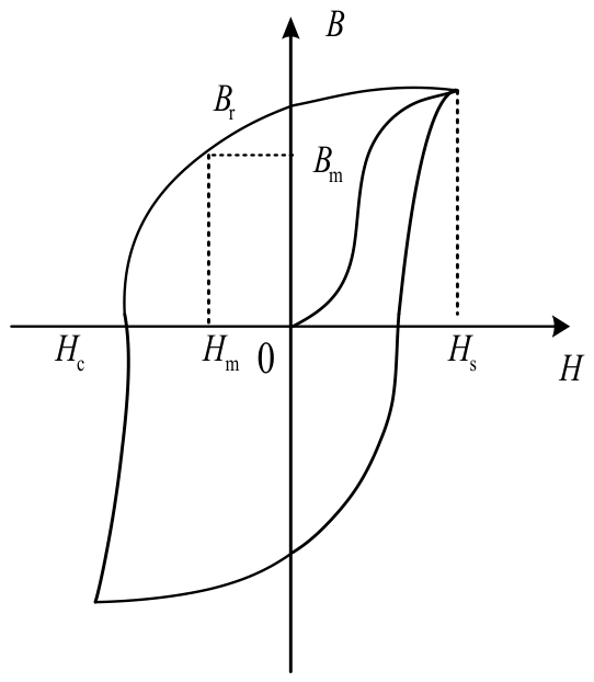
PM materials can describe their magnetization characteristics through hysteresis loops. The hysteresis loop of a PM is shown in Figure 1, which describes the relationship between flux intensity B and magnetic field intensity H. In Figure 1, Hs is the saturation magnetic field strength, when the magnetization strength is equal to or exceeds the saturation magnetic field strength of the PM material. The loop at this time is called the hysteresis loop. The larger the area enclosed by the loop, the more stable the magnetic properties of the PM material.

The demagnetization curve of PM materials is the curve of hysteresis loop in the second quadrant. As shown in Figure 1, the flux intensity Bm and the absolute values of magnetic field intensity Hm on the demagnetization curve are inversely proportional, and the directions of B_m and H_m are opposite, which indicates that the PM is a magnetic source, equivalent to the power supply in the circuit. The magnetic properties of PM materials need to be represented by two parameters: remanence and coercivity. The intersection point of the hysteresis loop and the H-negative half axis is the coercivity H_c. The intersection point between the hysteresis loop and the positive half axis of flux density B is the remanent magnetization B_r. The greater the remanence B_r and coercivity H_c of the PM material, the better the magnetic properties.

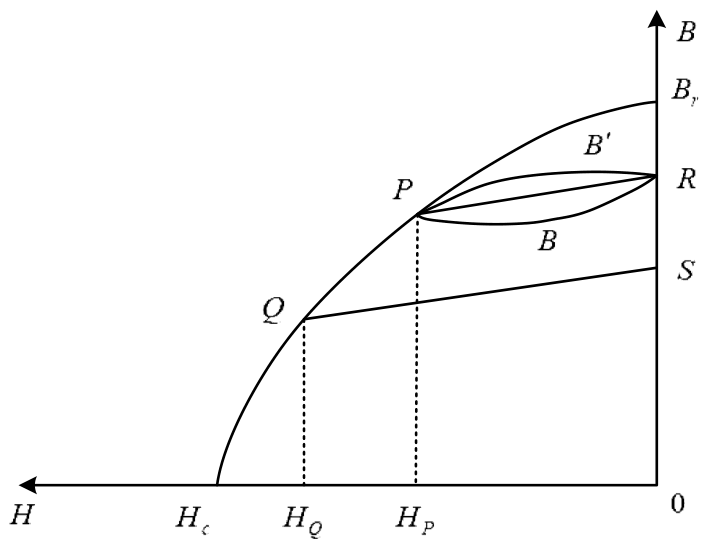
In practical applications, the magnetic field strength experienced by the PM does not change in a single direction, and the direction of magnetic field strength will constantly change. As shown in Figure 2, when the reverse magnetic field strength applied to the PM is H_P, the flux density of the PM will move down along the demagnetization curve B_rP. When the point of P is reached, the magnetic field is removed, and the flux density will not return to the point of (0, B_r) along the PB_r curve, but will move up to the point of R along the PBR curve. If a reverse magnetic field is applied again, then the flux density will decrease along the curve of RB’P. After repeating this several times, a small local hysteresis loop will be formed, which can be approximated by a straight line with PR, called the recovery line. When point P is the initial point, if the reverse magnetic field strength experienced by the PM again is less than the magnetic field strength corresponding to point of P, then the flux density will undergo reciprocating changes along the PR recovery line. On the contrary, the flux density will move downwards along PQ curve, and the flux density will change along QS recovery line. In this way, the PM will lose some magnetic energy, causing unstable motor performance and increasing the complexity of electromagnetic design for PMSMs.

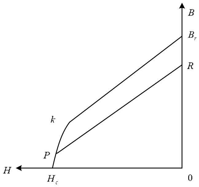
In general, the demagnetization curve of PM materials is a straight line, and PMs will not demagnetize. However, the demagnetization curves of some PM materials ferrite and NdFeB working in high-temperature environments are no longer a straight line. When the reverse magnetic field strength applied to the PM exceeds a certain value, the flux density will sharply decrease. The point where the magnetic flux density begins to sharply decrease in the demagnetization curve is called knee point, as shown at point k in Figure 3. When the demagnetization magnetic field strength does not exceed knee point magnetic field strength, the demagnetization curve is a straight line. When the demagnetization field strength exceeds the magnetic field strength corresponding to the knee point k, the demagnetization curve is no longer a straight line, and the PM will lose some magnetic energy.

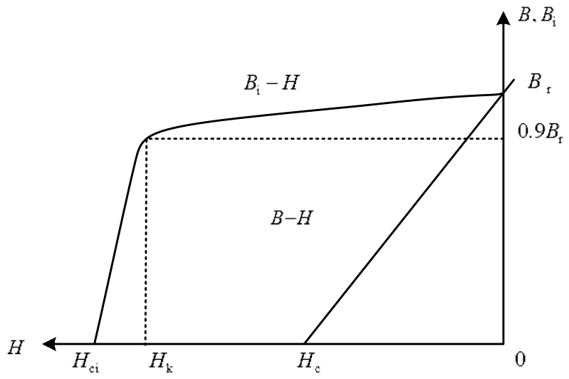
The intrinsic demagnetization curve characterizes intrinsic magnetic properties of PM materials, describing the relationship between the intrinsic flux intensity B_i and magnetic field intensity H. The relationship between demagnetization curve and the intrinsic demagnetization curve is shown in Figure 4. The intrinsic coercivity H_ci is the intersection point of the intrinsic demagnetization curve and the H-axis, and its value reflects the ability of anti-demagnetization of the PM. The larger the intrinsic coercivity, the less likely the PM is to undergo irreversible demagnetization. For PM materials with NdFeB, there is a significant difference between their demagnetization curve and intrinsic demagnetization curve, with H_ci being much greater than H_c. The greater the difference, the better the magnetic properties of the PM material.

According to the theory of ferromagnetism:

$$\overrightarrow{B}={\mu }_0\overrightarrow{H}$$

(1)

where μ₀ is the vacuum magnetic permeability.

In PM materials:

$$\overrightarrow{B}={\mu }_0\overrightarrow{H}+{\mu }_0\overrightarrow{M}$$

(2)

where M is magnetization strength of the PM material.

If the PM material is uniform, then Equation (2) can be further expressed as:

$$B={\mu }_{0}H+{\mu }_{0}M$$

(3)

B_i can be represented as:

$$B_i={\mu }_{0}M$$

(4)

By specifying the strength of the reverse magnetic field as a positive value, the relationship between demagnetization curve and intrinsic demagnetization curve can be obtained from Equation (3) as follows:

$$B_i=B+{\mu }_{0}H$$

(5)

In order to ensure the long-term stable operation of PMSMs, the magnetic properties of PMs need to be kept stable. It is necessary for PM materials to ensure chemical stability, time stability, magnetic stability, thermal stability, etc. Among them, thermal stability is the most important factor to consider for PM materials with NdFeB. Thermal stability reflects degree of influence of temperature on the magnetism of PM materials. When the temperature increases, the magnetic properties of PM materials will decrease. The decreased magnetic properties can be divided into two situations: recoverable and unrecoverable. When the magnetic properties can be restored to their initial state after temperature recovery, it is called reversible loss. This reversible change in magnetic properties caused by temperature is usually represented by the temperature coefficient.

The temperature coefficient α_Br can be expressed as:

$${\alpha }_{B_r}={\displaystyle \frac{B_1-{B^{\prime }}_0}{{B_0}^{\prime }\left(T_1-T_0\right)}}\times 100$$

(6)

The temperature coefficient α_Hci can be expressed as:

$${\alpha }_{H_{ci}}={\displaystyle \frac{H_{ci}-{H^{\prime }}_{ci}}{{H^{\prime }}_{ci}-\left(T_1-T_0\right)}}\times 100$$

(7)

Irreversible loss refers to the portion of magnetic performance loss in PM materials after the temperature returns to its initial value. The irreversible loss rate I_L can be expressed as follows:

$$I_L={\displaystyle \frac{{B^{\prime }}_0-B_0}{B_0}}\times 100$$

(8)

2.2. Demagnetization Mechanism of PM Materials

The demagnetization methods of PMs in IPMSMs for electric vehicles mainly include high-temperature demagnetization, AC demagnetization, and DC demagnetization, which are determined by the performance of PM materials with NdFeB. At different temperatures, the demagnetization curve of PMs varies. As the temperature increases, the knee point of demagnetization curve shifts upward, making PMs more prone to irreversible demagnetization [25]. The exchange of demagnetization magnetic fields will continuously change the magnetic domain structure of PMs, thereby reducing the residual flux intensity, and the higher the frequency of the alternating magnetic field, the greater the loss of magnetic energy [26]. PMs may undergo irreversible demagnetization when subjected to external magnetic fields, high temperatures, severe vibrations, chemical reactions, etc. At the same time, unreasonable structure design, poor manufacturing, and the magnetic properties of the PM material itself can all cause irreversible demagnetization [27].

During the starting process of a PMSM and the occurrence of a short-circuit fault, a large current flows through the stator winding, of which demagnetization current accounts for a large proportion, thereby generating a large demagnetization magnetic field. When the demagnetization magnetic field strength exceeds a certain limit, the domain walls and magnetic moments of the PM magnetic domains change. Even if the demagnetization magnetic field is removed, the magnetic domains of PMs cannot return to their initial state, resulting in the irreversible demagnetization of PMs. Any microscopic particle is in thermal motion at any time, and the thermal motion of atoms inside a PM will constantly change the direction of the magnetic moment. When the working temperature of the PM is low, the effect of atomic thermal motion is not significant. When the temperature rises to a certain degree, atomic thermal motion inside the PM is intense, causing some magnetic domain arrangements to be disordered, resulting in irreversible demagnetization [28].

After the PMSM is subjected to severe vibration impact, it may cause changes in the magnetic domain structure and magnetic moment direction inside the PM, resulting in a deterioration of its magnetic properties and even demagnetization. When PMs are subjected to chemical reactions such as salt alkali, acid, oxygen, etc., their surface and internal chemical structures will change, causing irreversible demagnetization. Therefore, various protective measures need to be taken for PMs during manufacturing to prevent chemical corrosion. Generally, the corrosion resistance is improved by adding protective coatings on the surface of PMs, such as galvanizing, nickel plating, and electrophoresis. The reasons for demagnetization of PMs vary depending on the application scenarios of PMSMs. When PMSMs are applied to aircraft, temperature, vibration, and other factors are the main causes of demagnetization. When applied to electric vehicles, temperature and external magnetic field are the main causes of demagnetization. For IPMSMs used in vehicles with high power density, small size, difficulty in heat dissipation, large armature reaction, temperature, and external magnetic field are the main reasons for demagnetization.

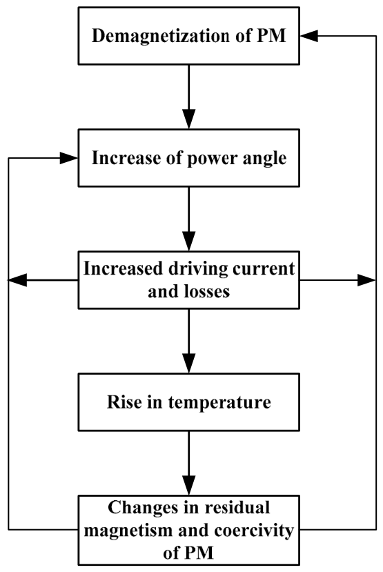
The demagnetization fault of a PM can cause a decrease in no-load back EMF. In order to maintain a balance between the electromagnetic torque and load torque of IPMSMs, the IPMSM will automatically increase the current angle θ, resulting in an increase in the stator winding current, motor losses, and internal temperature of the IPMSM. The increase in the working temperature of the PM will change the magnetic parameters of PMs, causing magnetic energy loss of PMs. This will form a vicious cycle inside the IPMSM. The demagnetization process diagram is shown in Figure 5. So, the research on demagnetization of IPMSMs is very important. For the IPMSMs in the drive system of electric vehicles, the main reasons for demagnetization are demagnetization magnetic field and temperature rise.

3. Calculation of Parameters

3.1. Resistance Value of Stator Winding

The formula for calculating phase resistance of stator winding can be expressed as follows:

$$R={\rho }_{cu}{\displaystyle \frac{2N{l}_c}{s_{c}a}}$$

(9)

where ρ_cu is the resistivity of copper wire; s_c, l_c, and N are the cross-sectional area of stator winding coil, average half turn length, and number of series turns per phase, respectively.

At different temperatures, the resistivity of copper wire varies. Within a certain temperature range, the resistivity of copper wire is proportional to temperature. Refer to the manual to obtain resistivity of copper wire at different temperatures. After calculation, the resistance values of each phase of stator winding at different temperatures are shown in

Table 1. Resistance of stator winding at different temperatures.

T/°C	R/Ω	T/°C	R/Ω
0	0.046	60	0.059
10	0.048	70	0.062
20	0.050	75	0.063
30	0.052	80	0.064
40	0.055	90	0.066
50	0.057	100	0.069

. When the armature current is small, the temperature of stator winding is not high, and the resistance value is also small. The copper loss generated by IPMSMs is small, but as the current increases, the temperature also increases, and the copper wire resistance increases, making copper loss the main loss in the constant-torque region of IPMSMs.

3.2. d–q-Axis Inductance

ABC stationary coordinate system; the inductance of IPMSMs can be expressed as follows:

$$L=\left[\begin{array}{ccc}{L}_{\mathrm{AA}}& M_{\mathrm{AB}}& M_{\mathrm{AC}}\\ M_{\mathrm{BA}}& L_{\mathrm{BB}}& M_{\mathrm{BC}}\\ M_{\mathrm{CA}}& M_{\mathrm{CB}}& L_{\mathrm{CC}}\end{array}\right]$$

(10)

The self-inductance and mutual inductance of three-phase winding can be represented as follows:

$$\begin{array}{l}{L}_{AA}=L_{s0}+L_{s2}\cos 2\xi \\ L_{BB}=L_{s0}+L_{s2}\cos 2\left(\xi -{120}^{\circ }\right)\\ L_{CC}=L_{s0}+L_{s2}\cos 2\left(\xi +{120}^{\circ }\right)\end{array}$$

(11)

$$\begin{array}{l}{M}_{BC}=M_{BC}=-M_{s0}+M_{s2}\cos 2\xi \\ M_{AC}=M_{AC}=-M_{s0}+M_{s2}\cos 2\left(\xi -{120}^{\circ }\right)\\ M_{BA}=M_{AB}=-M_{s0}+M_{s2}\cos 2\left(\xi +{120}^{\circ }\right)\end{array}$$

(12)

where

$$\begin{array}{l}{M}_{\mathrm{s}0}\approx {\displaystyle \frac{1}{2}}{L}_{\mathrm{s}0}\\ M_{\mathrm{s}2}\approx L_{\mathrm{s}2}\end{array}$$

(13)

where L_S0 and L_S2, respectively, represent the average self-inductance of stator winding and amplitude of the second harmonic; M_S0 and M_S2 are average mutual inductance and second harmonic amplitude of stator winding, respectively, ξ is the angle between d-axis of rotor and A-phase axis of stator winding.

The 3s-2r transformation of stator flux linkage can be expressed as follows:

$$\left[\begin{array}{c}{\psi }_d\\ {\psi }_q\\ 0\end{array}\right]=C_{3\mathit{s-}2r}\left[\begin{array}{c}{\psi }_A\\ {\psi }_B\\ {\psi }_C\end{array}\right]$$

(14)

In three-phase ABC stationary coordinate system, the flux linkage for each phase of stator can be expressed as:

$$\left[\begin{array}{c}{\psi }_A\\ {\psi }_B\\ {\psi }_C\end{array}\right]=\left[\begin{array}{ccc}{L}_{AA}& M_{AB}& M_{AC}\\ M_{BA}& L_{BB}& M_{BC}\\ M_{CA}& M_{CB}& L_{CC}\end{array}\right]\left[\begin{array}{c}{i}_A\\ i_B\\ i_C\end{array}\right]+\left[\begin{array}{c}{\psi }_{\mathrm{f}A}\\ {\psi }_{\mathrm{f}B}\\ {\psi }_{\mathrm{f}C}\end{array}\right]$$

(15)

where ψ_fA, ψ_fB, and ψ_fC are components of PM flux linkage in the ABC stationary coordinate system.

$$\left[\begin{array}{c}{i}_A\\ i_B\\ i_C\end{array}\right]={C_{3\mathit{s-}2r}}^{-1}\left[\begin{array}{c}{i}_q\\ i_d\\ 0\end{array}\right]$$

(16)

From Equations (14) to (16), the flux linkage in d–q coordinate system can be obtained as:

$$\left[\begin{array}{c}{\psi }_d\\ {\psi }_q\\ 0\end{array}\right]=C_{3\mathit{s-}2r}\left[\begin{array}{ccc}{L}_{AA}& M_{AB}& M_{AC}\\ M_{BA}& L_{BB}& M_{BC}\\ M_{CA}& M_{CB}& L_{CC}\end{array}\right]{C_{3\mathit{s-}2r}}^{-1}\left[\begin{array}{c}{i}_q\\ i_d\\ 0\end{array}\right]+C_{3\mathit{s-}2r}\left[\begin{array}{c}{\psi }_{\mathrm{f}A}\\ {\psi }_{\mathrm{f}B}\\ {\psi }_{\mathrm{f}C}\end{array}\right]$$

(17)

In dq0 coordinate system:

$$\left[\begin{array}{c}{\psi }_d\\ {\psi }_q\\ 0\end{array}\right]=\left[\begin{array}{ccc}{L}_d& 0& 0\\ 0& L_q& 0\\ 0& 0& 0\end{array}\right]\left[\begin{array}{c}{i}_q\\ i_d\\ 0\end{array}\right]+\left[\begin{array}{c}{\psi }_{\mathrm{f}}\\ 0\\ 0\end{array}\right]$$

(18)

From Equations (17) and (18), it can be concluded that:

$$\left[\begin{array}{ccc}{L}_d& 0& 0\\ 0& L_q& 0\\ 0& 0& 0\end{array}\right]=C_{3\mathit{s-}2r}\left[\begin{array}{ccc}{L}_{AA}& M_{AB}& M_{AC}\\ M_{BA}& L_{BB}& M_{BC}\\ M_{CA}& M_{CB}& L_{CC}\end{array}\right]{C_{3\mathit{s-}2r}}^{-1}$$

(19)

Under constraint of equal power conditions, the transformation matrix can be expressed as follows:

$$C_{3\mathit{s-}2r}=\sqrt{{\displaystyle \frac{2}{3}}}\left[\begin{array}{ccc}\cos \xi & \cos \left(\xi -{120}^{\circ }\right)& \cos \left(\xi +{120}^{\circ }\right)\\ -\sin \xi & -\sin \left(\xi -{120}^{\circ }\right)& -\sin \left(\xi +{120}^{\circ }\right)\\ {\displaystyle \frac{1}{\sqrt{2}}}& {\displaystyle \frac{1}{\sqrt{2}}}& {\displaystyle \frac{1}{\sqrt{2}}}\end{array}\right]$$

(20)

$${C_{3\mathit{s-}2r}}^{-1}\sqrt{{\displaystyle \frac{2}{3}}}\left[\begin{array}{ccc}\cos \xi & -\sin \xi & {\displaystyle \frac{1}{\sqrt{2}}}\\ \cos \left(\xi -{120}^{\circ }\right)& -\sin \left(\xi -{120}^{\circ }\right)& {\displaystyle \frac{1}{\sqrt{2}}}\\ \cos \left(\xi +{120}^{\circ }\right)& -\sin \left(\xi +{120}^{\circ }\right)& {\displaystyle \frac{1}{\sqrt{2}}}\end{array}\right]$$

(21)

From Equations (19)–(21), d–q-axis inductance can be expressed as:

$$\begin{array}{l}{L}_q={\displaystyle \frac{3}{2}}\left(L_{s0}+L_{s2}\right)\\ L_d={\displaystyle \frac{3}{2}}\left(L_{s0}-L_{s2}\right)\end{array}$$

(22)

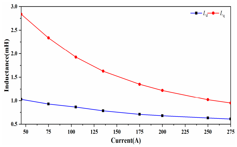
The d–q-axis inductance of the IPMSM does not always remain constant. When stator winding current changes, d–q-axis inductance also changes accordingly. The values of d–q-axis inductance with different current excitations applied to the stator winding are shown in

Table 2. d–q-axis inductance under different currents.

Current Amplitude/A	Ld/mH	Lq/mH
45	1.027	2.837
75	0.927	2.335
105	0.863	1.925
135	0.784	1.628
175	0.709	1.35
200	0.678	1.22
250	0.631	1.02
275	0.61	0.95

, and the relationship between d–q-axis inductance and stator current is shown in Figure 6.

According to Table 2 and Figure 6, it can be seen that the q-axis inductance L_q of the IPMSM is greater than the d-axis inductance L_d, which is determined by the structure of the IPMSM. As the stator winding current continues to increase, both d-axis inductance and q-axis inductance show a decreasing trend. As the stator winding current increases, the q-axis magnetic circuit gradually saturates, and the decrease speed of q-axis inductance slows down. At the same time, the salient pole ratio of the IPMSM also decreases with increase in current. At rated current, the salient pole ratio of the IPMSM is 1.56. The impact of cross-axis inductance on the performance of the IPMSM is relatively small, while the impact of direct-axis inductance on the performance of the IPMSM is significant.

3.3. No-Load Back EMF

No-load back EMF E₀ is the induced voltage in stator winding by the fundamental magnetic flux of the no-load air gap generated only by the PM of the rotor in the absence of the driving current of the IPMSM. It can well reflect the working state of the IPMSM and can affect its static and dynamic performance. The no-load back EMF can be expressed as follows:

$$\begin{array}{cc}\hfill E_0& =4.44f{K}_{dp}N{\varphi }_{10}\hfill \\ & =4.44f{K}_{dp}N{\varphi }_{\delta 0}{K}_f\hfill \\ & =4.44f{K}_{dp}N{K}_f{\displaystyle \frac{b_{m0}{B}_r{A}_M}{{\sigma }_0}}\times {10}^{-4}\hfill \end{array}$$

(23)

where K_dp is the factor of winding; K_f is the waveform coefficient of the air gap magnetic field; δ is air gap length; σ₀ is the coefficient of no-load leakage; b_m0 is the amplitude of the fundamental flux density of the PM; N is the number of turns in series for each phase winding; f is the fundamental frequency; ${\varphi }_{10}$ is the air gap flux per pole; ${\varphi }_{\delta 0}$ is the no-load main air gap flux; B_r is the residual flux density of the PM; A_M provides the magnetic flux area per pole for PMs, and the rotor magnetic circuit of the IPMSM is radial. Therefore, A_M can be expressed as follows:

$$A_M=b_M{L}_M$$

(24)

where b_M and L_M are the magnetic pole width and axial length of the PM, respectively.

$$K_f={\displaystyle \frac{8}{{\pi }^2{\alpha }_i}}\sin {\displaystyle \frac{{\alpha }_i\pi }{2}}$$

(25)

The calculation pole arc coefficient α_i can be expressed as:

$${\alpha }_i={\displaystyle \frac{b+2\delta }{{\tau }_1}}$$

(26)

where b is the arc length of the pole shoe; τ₁ is the distance of the stator pole.

According to Equation (23), the magnitude of no-load back EMF E₀ is related to the residual flux intensity B_r, and E₀ is directly proportional to the residual magnetic Br. The residual magnetism of the demagnetization curve varies with different working temperatures of the PM, and the higher the temperature, the smaller the residual magnetism. The effective values of no-load back EMF of the IPMSM under different temperature demagnetization curves can be obtained from Equations (24)–(26) and finite element analysis, as shown in

Table 3. Effective value of no-load back EMF at different temperatures.

T/°C	E0/V
20	266.04
50	255.23
80	243.45
100	236.56
120	225.50
150	215.18

.

3.4. Flux Linkage Analysis of PMs

The flux linkage of PMs can be expressed as:

$${\psi }_f={\displaystyle \frac{E_0}{\sqrt{2}\pi f}}$$

(27)

In Section 3.3, the values of no-load back EMF at various temperatures have been obtained. As shown in Equation (27), the frequency remains constant, and the flux linkage of PMs is proportional to no-load back EMF E₀. The flux linkage values of PMs at different temperatures are shown in

Table 4. Flux linkage values of PMs at different temperatures.

T/°C	ψf/Wb
20	0.142
60	0.135
90	0.127
110	0.123
130	0.118
150	0.111

.

3.5. Analysis of Electromagnetic Torque

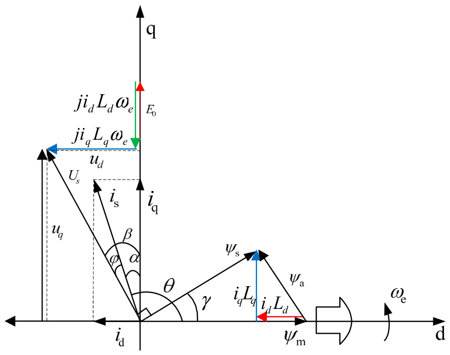
The vector diagram in the d–q coordinate system during the steady-state operation of the IPMSM is shown in Figure 7. In Figure 7, the angle between the stator voltage space vector u_s and the q-axis is the voltage angle β. The angle between the stator current space vector and the d-axis is the current control angle θ, which ranges from 0° to 180°. The power factor angle φ is the angle between the stator voltage space vector u_s and the stator current space vector i_s.

When the IPMSM runs stably, the input power P₁ can be expressed as follows:

$$P_1=m{U}_s{\displaystyle \frac{E_0\left(X_q\sin \theta -R_1\cos \theta +R_1{U}_s\right)}{{R_1}^2+X_d{X}_q}}+{\displaystyle \frac{1}{2}}m{U_s}^2{\displaystyle \frac{E_0\left(X_d-X_q\right)\sin 2\theta }{{R_1}^2+X_d{X}_q}}$$

(28)

Ignoring the stator resistance, the electromagnetic power Pem can be approximately expressed as:

$$P_{em}\approx P_1\approx {\displaystyle \frac{m{U}_s{E}_0}{X_d}}\sin \theta +{\displaystyle \frac{1}{2}}m{U_s}^2\left({\displaystyle \frac{1}{X_q}}-{\displaystyle \frac{1}{X_d}}\right)\sin 2\theta$$

(29)

The electromagnetic torque T_em of the IPMSM can be obtained from Equation (29) as follows:

$$\begin{array}{cc}\hfill T_{em}& ={\displaystyle \frac{P_{em}}{\Omega }}={\displaystyle \frac{mp{U}_s{E}_0}{\omega X_d}}\sin \theta +{\displaystyle \frac{mp{U_s}^2}{2\omega }}\left({\displaystyle \frac{1}{X_q}}-{\displaystyle \frac{1}{X_d}}\right)\sin 2\theta \hfill \\ & =T_{\mathrm{mag}}+T_{\mathrm{rel}}\end{array}$$

(30)

where Ω is mechanical angular velocity of the IPMSM.

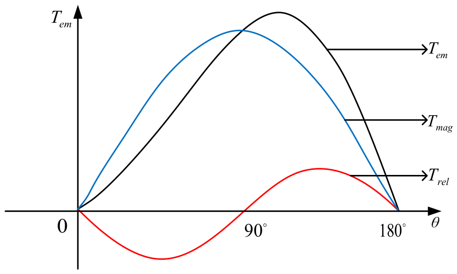
The relationship between electromagnetic synthesis torque T_em, permanent magnet torque T_mag, reluctance torque T_rel, and current control angle θ can be obtained from Equation 30, as shown in Figure 8. Permanent magnet torque is torque formed by the interaction between the air gap magnetic field generated by the PM and the stator armature reaction magnetic field. The reluctance torque is torque caused by asymmetric magnetic circuit of rotor, which is the reactive torque of the IPMSM. The reluctance torque is a negative sine function, and the electromagnetic torque of maximum value corresponds to a current control angle θ greater than 90°.

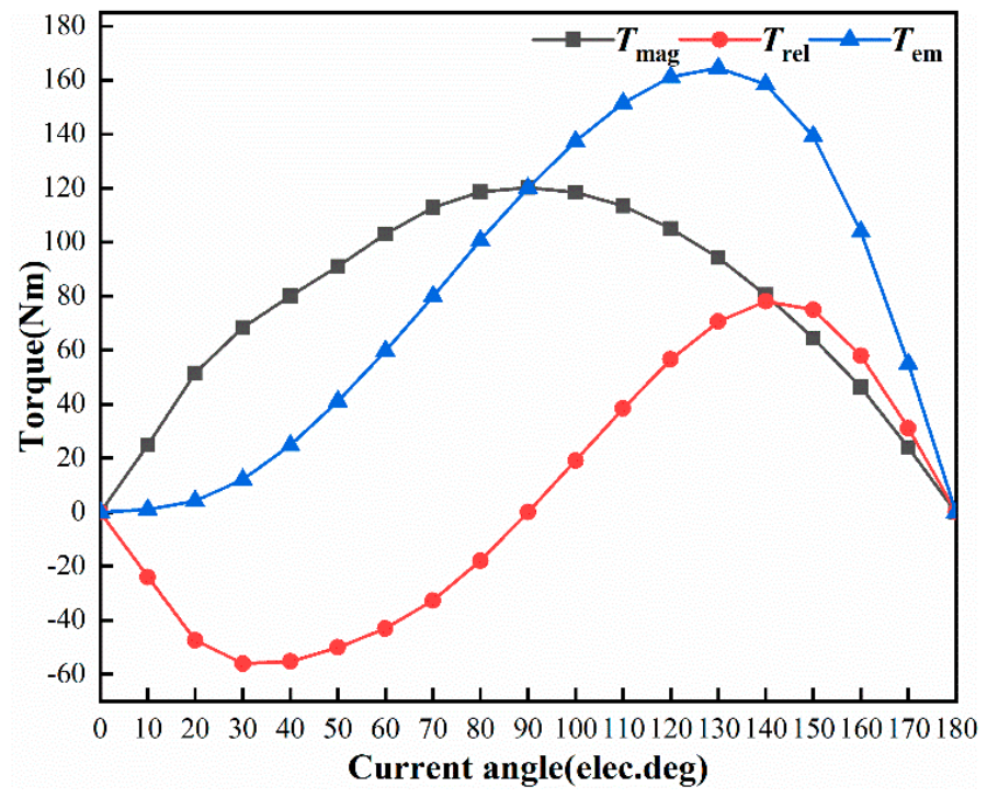
The finite element simulation results of the relationship between T_mag, T_rel, T_em, and current control angle θ of the IPMSM under rated operating conditions with a sine current amplitude of 275 A, current control angle of 120°, and speed of 4000 rpm are shown in Figure 9. The finite element simulation results of the torque of the IPMSM shown in Figure 9 are consistent with theoretical analysis results in Figure 8, further proving the correctness of theoretical analysis.

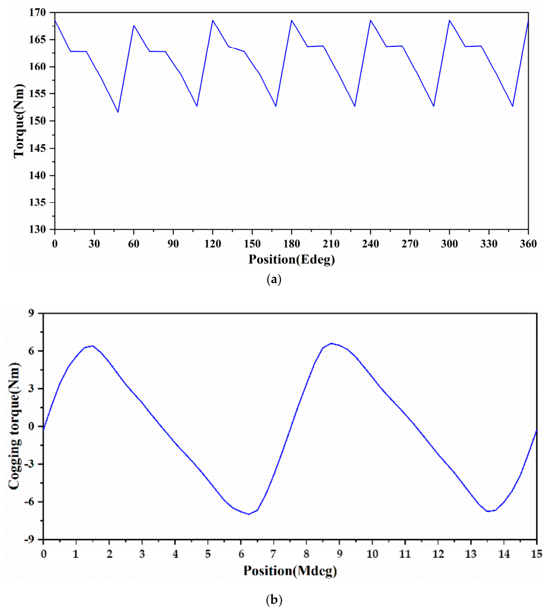
Under rated operating conditions, the output torque and cogging torque of the IPMSM are shown in Figure 10. From Figure 10a, it can be seen that the average output torque is 161.2 Nm. Due to the presence of cogging torque, the torque ripple of the IPMSM is relatively large, with a torque ripple reaching 17 Nm and a torque ripple ratio of 10.5%. From Figure 10b, it can be seen that the peak-to-peak cogging torque can reach 13.6 Nm.

4. Iterative Temperature Rise Analysis and Calculation of Electromagnetic–Thermal Field Coupling

The electromagnetic load of high-power-density vehicle motors generally tends to the limit, increasing the losses and heat generation, making the calculation of temperature rise of each component an important consideration in the design of vehicle motors. The increase in temperature leads to an increase in the resistivity of copper wire in the winding, which in turn increases the copper loss under the same driving current. As the temperature increases, the magnetic properties of the PM decrease or irreversible demagnetization occurs, which leads to a decrease in the air gap flux density. Under the same torque output conditions, the driving current increases, resulting in an increase in copper loss. The increase in copper loss further leads to an increase in the temperature of winding and the PM. Therefore, the electromagnetic thermal coupling model is very necessary for motor design and drive simulation.

4.1. Design Parameters of IPMSM

The parameters of the IPMSM are shown in

Table 5. Design parameters of IPMSM.

Parameters	Values	Parameters	Values
Rated power (kW)	66	Peak power (kW)	130
Rated speed (rpm)	4000	Maximum speed (rpm)	13,000
Bus DC voltage (V)	500	Pole–slot combination	48S8P
Stator and rotor materials	M350-50A	PM model	N30UH
Slot depth(mm)	21	Stator outer diameter (mm)	198
Tooth width (mm)	4.15	Stator bore (mm)	132
Rated current amplitude (A)	275	Peak current amplitude (A)	500
PM width of first layer (mm)	21.3	PM width of second layer (mm)	13.9
PM thickness of first layer (mm)	7.65	PM thickness of second layer (mm)	3.86

. The pole slot is matched with 8 poles and 48 slots, and the stator adopts short-distance distributed winding. The rated current amplitude is 275 A, the peak current amplitude is 500 A, and the cooling method of motor is liquid cooling. Adopting housing water jacket, the liquid cooling is water, the inlet temperature of liquid cooling is 60 °C, and the flow rate of liquid cooling is 6.5 L/min.

4.2. Influence of Winding Temperature on Electromagnetic Performance

The resistivity of copper wire increases with temperature, and the approximate linear relationship between copper wire resistivity and temperature is expressed as follows:

$${\rho }_{cu}={\rho }_0[1+{\alpha }_b(t-t_0)]$$

(31)

where ρ_cu is the copper wire resistivity, t₀ is the standard temperature, usually 20 °C, and ρ₀ is the copper wire resistivity at the standard temperature. α_b is the temperature coefficient of electrical resistivity of copper wire at standard temperature, and t is the specific temperature of winding with copper wire.

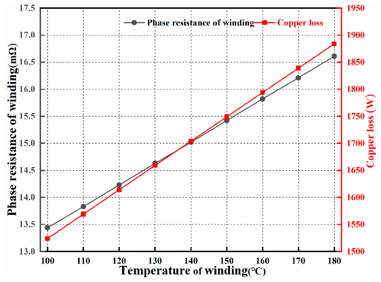
The resistivity of copper wire increases with the rise in winding temperature, that is, the phase resistance of winding increases with temperature, and when the driving current is constant, the copper loss of winding increases with winding temperature. The influence of winding temperature on electromagnetic performance is shown in Figure 11. From Figure 11, it can be observed that as the winding temperature increases, the phase winding resistance increases linearly. Under the same driving current, the copper loss also increases linearly with the temperature, and the increase in copper loss further increases winding temperature. To accurately calculate copper loss and winding temperature rise, it is necessary to consider the mutual influence between the electromagnetic and thermal field.

4.3. Influence of PM Temperature on Electromagnetic Performance

In order to improve the torque density of IPMSMs, high-performance neodymium iron boron PMs are generally selected, and the magnetic properties of PMs decrease with increasing temperature. The residual flux density B_r and its calculated coercive force at operating temperature can be calculated according to Equations (32) and (33).

$$B_{rT}=[1+(t-20){\displaystyle \frac{{\alpha }_{B_r}}{100}}](1-{\displaystyle \frac{L_1}{100}})B_{r20}$$

(32)

$$H_{cT}=[1+(t-20){\displaystyle \frac{{\alpha }_{H_c}}{100}}](1-{\displaystyle \frac{L_1}{100}})H_{c20}$$

(33)

where α_Br is the reversible temperature coefficient of residual magnetic flux density B_r of PMs, L₁ is the irreversible demagnetization rate of residual magnetic flux density, and B_r20 is the residual magnetic flux density of PMs at a temperature of 20 °C. α_Hc is the calculated coercivity H_c temperature coefficient for PMs, and H_c20 is the calculated coercivity of PMs at a temperature of 20 °C.

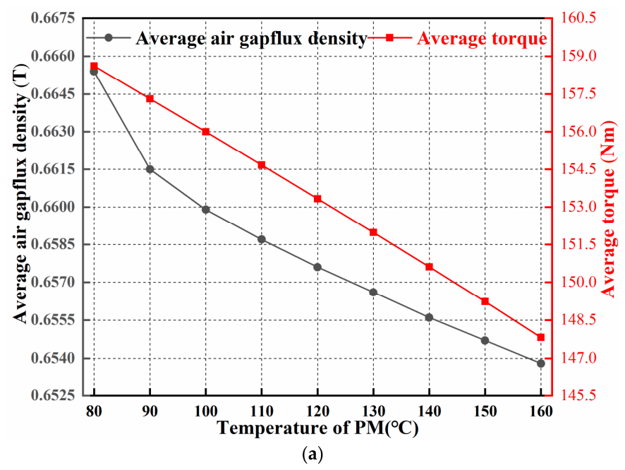
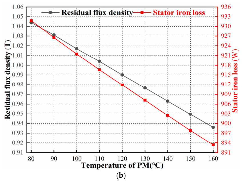
The effect of the temperature rise of PMs on electromagnetic performance is shown in Figure 12. It can be observed from Figure 12 that the residual flux density of PMs and the air gap flux density of the motor decrease with the increase in PM temperature, which leads to a decrease in output torque and iron loss. This is because when the temperature of the PM increases, the residual magnetism of the PM will decrease, resulting in a decrease in the motor’s output torque capacity and iron loss. Therefore, under the same torque constraint, it is necessary to increase the driving current, further increasing copper loss and temperature rise. This will further increase the phase resistance of the winding, which will lead to a further increase in the temperature of winding and PMs in the rotor. In summary, changes in the temperature of PMs can cause variations in air gap flux density and various parts of the iron core, directly affecting the magnitude of torque and iron loss.

4.4. Temperature Rise Calculation of IPMSM with Electromagnetic Thermal Coupling

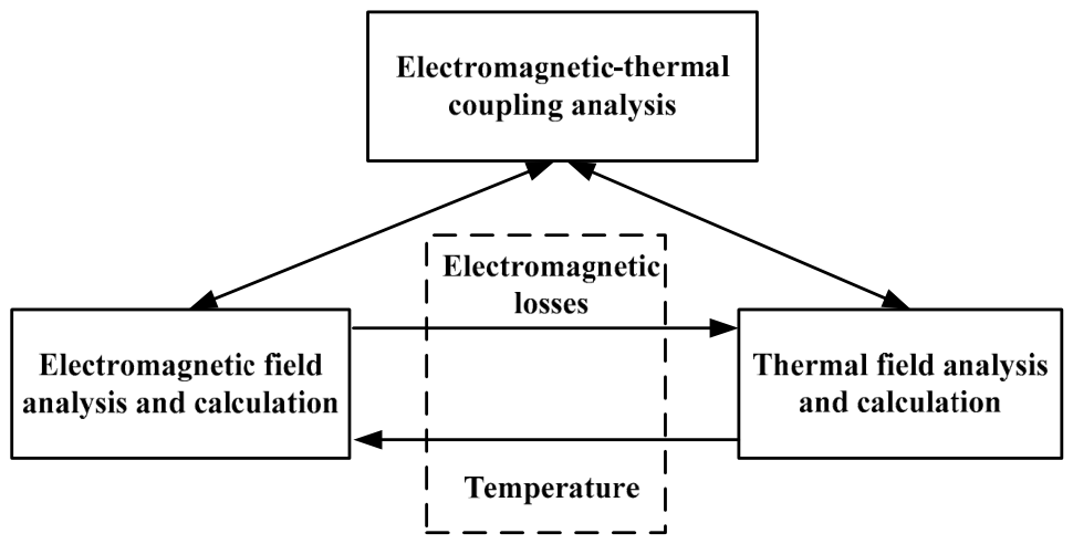
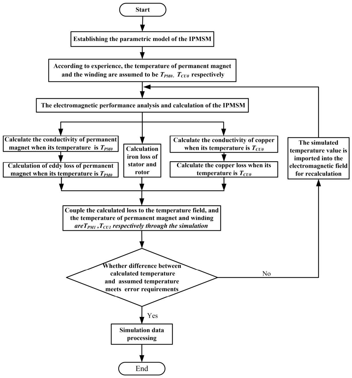
As mentioned above, when accurately calculating losses, the influence of temperature on various material properties must be considered. The electromagnetic field, temperature field, and stress field of high-torque-density permanent magnet synchronous motors change frequently, and the physical fields interact with each other. The schematic diagram of electromagnetic thermal coupling analysis and calculation is shown in Figure 13.

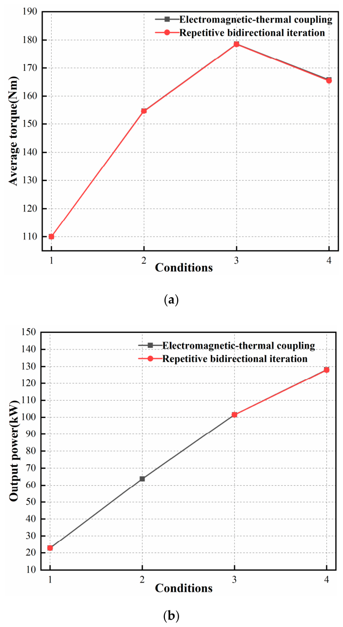
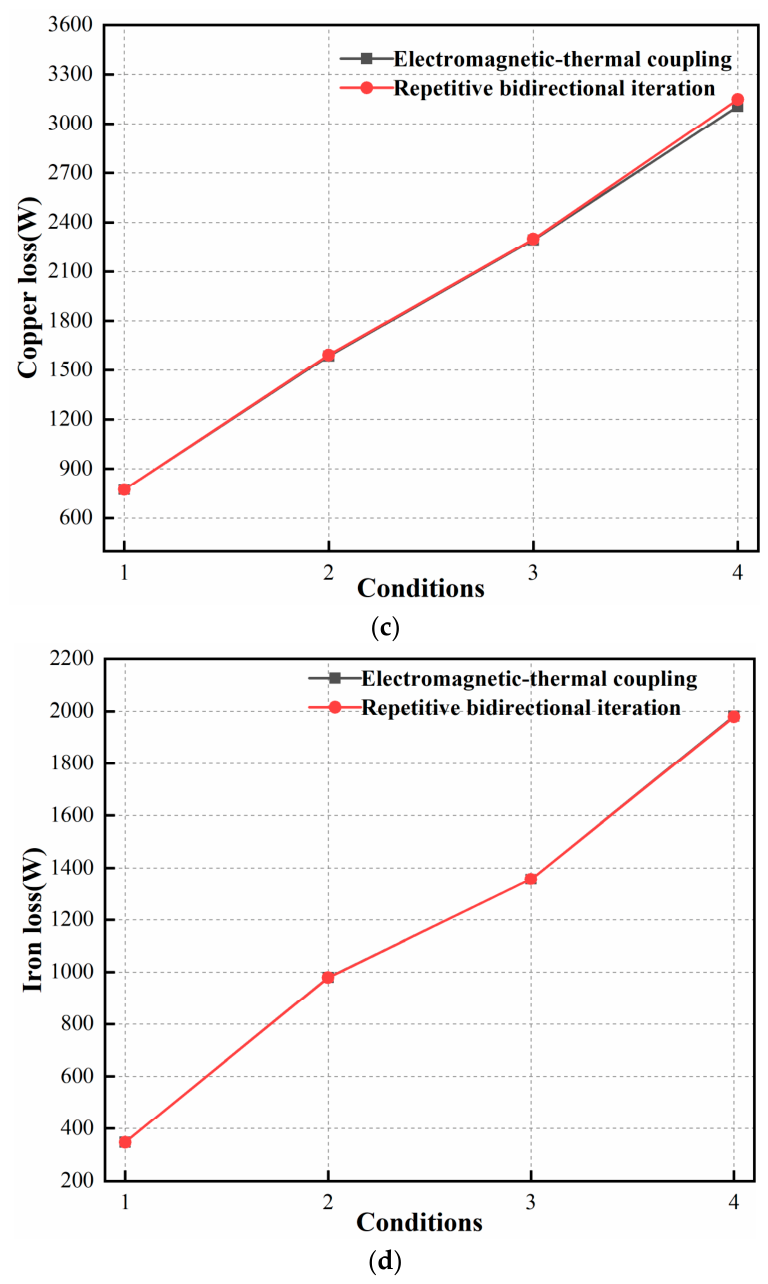
Under different operating conditions, the copper and iron losses of IPMSMs vary, so the temperature rise is also different. This paper selects four working conditions including urban low speed, urban medium speed, urban high speed, and ultra-high speed to analyze and calculate the temperature rise under different working conditions. The parameters of four working conditions with speed, phase current amplitude, and current angle are shown in

Table 6. Values of relevant parameters under different operating conditions.

Parameters	Speed (rpm)	Phase Current Amplitude (A)	Current Angle (Edeg)
Condition1	2000	200	110
Condition 2	4000	275	120
Condition 3	5500	320	140
Condition 4	7500	360	155

.

The temperature rise calculation flowchart of IPMSMs based on electromagnetic–thermal coupling is shown in Figure 14. As shown in Figure 14, the temperature rise calculation of the IPMSM first assumes the operating temperature of the PM and stator winding based on experience and calculates the loss. Next, the calculated loss-coupled temperature field is used to calculate the temperature of each component of the IPMSM. The final calculation of the temperature of each component is coupled back to the electromagnetic field based on the updated material characteristics to update the calculation of losses. The bidirectional iterative calculation between the electromagnetic and temperature field is repeated until the temperature meets the error requirements, and the iterative calculation is stopped.

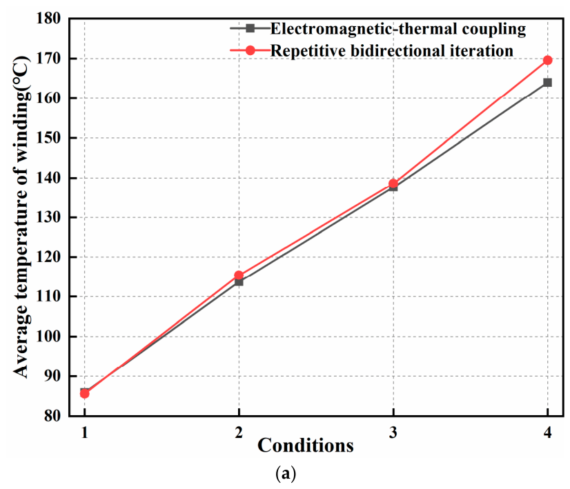
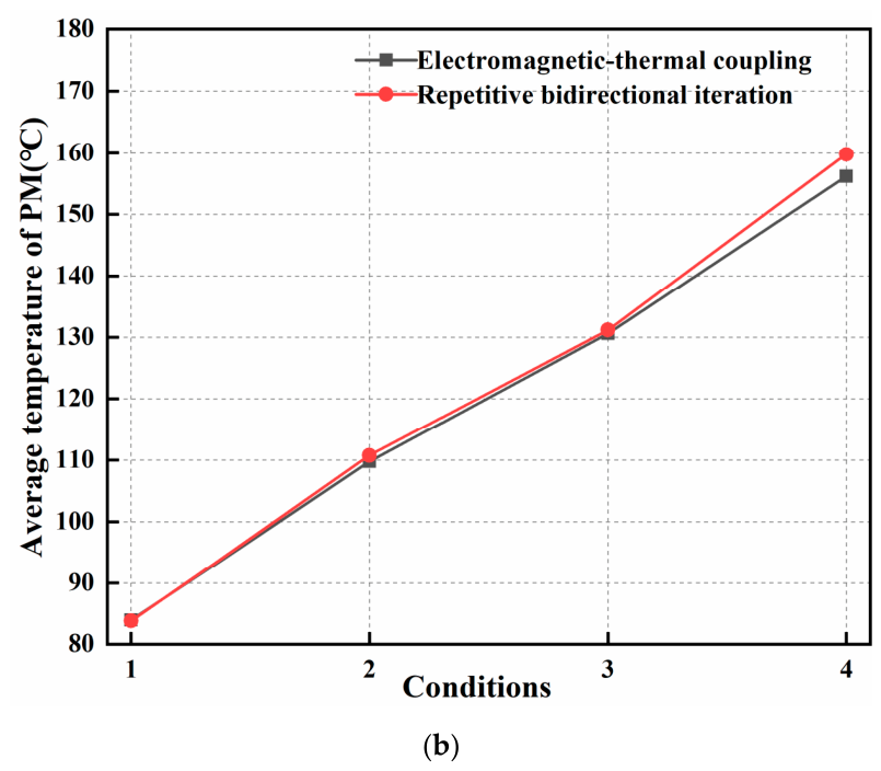
The temperature rise comparison of main components of motor under different operating conditions using electromagnetic–thermal coupling method and electromagnetic–thermal coupling combined with repeated bidirectional iteration method is shown in Figure 15. From Figure 15, it can be seen that under operating conditions 1, 2, and 3, as the drive current and speed are both relatively small, the copper and iron losses are relatively small, resulting in a lower temperature rise of winding and PM. The temperature rise calculated by electromagnetic–thermal coupling and electromagnetic–thermal coupling combined with repeated bidirectional iteration is basically the same, with small errors and a maximum error rate of 1.5%. Under operating condition 4, as the drive current and speed are both high, the copper and iron losses increase rapidly, resulting in a significant increase in the temperature rise of winding and PM. At this time, the temperature rise of electromagnetic–thermal coupling and electromagnetic–thermal coupling combined with repeated bidirectional iterative calculations is relatively large, with an error rate of 3.4%. In summary, it is necessary to accurately calculate the temperature rise of each component through electromagnetic–thermal coupling and repeated bidirectional iteration.

The main performance comparisons of electromagnetic–thermal coupling and electromagnetic–thermal coupling combined with repeated bidirectional iteration method for calculating the average torque, output power, copper and iron losses are shown in Figure 16. From Figure 16, it can be seen that under operating conditions 1, 2, and 3, the torque, output power, copper loss, and iron loss calculated by electromagnetic–thermal coupling method and electromagnetic–thermal coupling combined with repeated bidirectional iteration method are basically the same. Under operating condition 4, the results of electromagnetic–thermal coupling and electromagnetic–thermal coupling combined with repeated bidirectional iteration method have relatively large errors, with copper loss calculation having the largest error rate of 1%,which further indicates that using electromagnetic–thermal coupling combined with repeated bidirectional iteration method to calculate temperature rise is also necessary for accurately calculating torque, output power, copper loss and iron loss.

5. Simulation Analysis of PM Demagnetization

5.1. Basis for Demagnetization of PMs

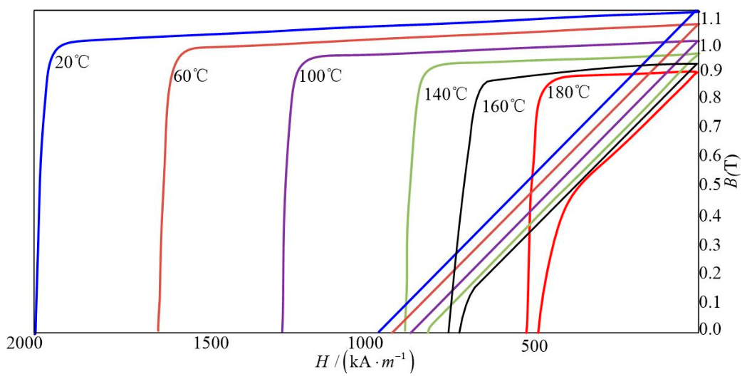
The PM material selected for the IPMSM in this paper is N30UH, and its demagnetization curve and intrinsic demagnetization curve at different temperatures are shown in Figure 17. N30UH has a remanent magnetization of B_r = 1.125 T, a coercivity of H_c = 852,616 A/m, an intrinsic coercivity of H_cj = 1,992,600 A/m, and a maximum operating temperature of 180 °C. When the working temperature of the PM is not higher than 140 °C, the demagnetization curve of N30UH is almost a straight line. After the demagnetization field withdraws, the PM will not produce magnetic energy loss. When the working temperature of the PM is greater than 140 °C, the demagnetization curve shows a clear knee point. If the demagnetization field strength exceeds knee point magnetic field strength, then the flux density of the PM will sharply decrease. After the demagnetization field withdraws, the residual magnetism cannot return to its original value, resulting in irreversible demagnetization. As the temperature increases, flux density corresponding to the knee point becomes higher, and the PM is more prone to irreversible demagnetization. The flux density values corresponding to knee points on the demagnetization curve of N30UH at 160 °C and 180 °C are 0.15 T and 0.34 T, respectively.

From the above analysis, it can be concluded that the demagnetization situation of the PM can be analyzed by analyzing the relationship between the working point of the PM and the knee point of the demagnetization curve. That is, by judging whether the flux density of the working point of the PM at any time is lower than the flux density of the corresponding temperature demagnetization curve of the knee point, it can be determined whether the PM has undergone irreversible demagnetization. This method is intuitive, but there is contingency in practical applications. It is possible to simulate the irreversible demagnetization of the PM as a whole or locally, analyze the changes in important performance parameters of the IPMSM after the PM undergoes irreversible demagnetization, and obtain the basis for determining whether the PM of the IPMSM undergoes irreversible demagnetization.

5.2. The Calculation of Working Point

According to the demagnetization curve of N30UH, it can be seen that below 100 °C, the demagnetization knee point is very low, and the probability of irreversible demagnetization is very small. However, at 160 °C and 180 °C, knee points of the demagnetization curve correspond to higher flux density values, and the probability of irreversible demagnetization is very high. By building a fault model of uniform demagnetization and local demagnetization of PMs under a demagnetization curve of 160 °C, the changes in magnetic cloud map, torque, and no-load back EMF after irreversible demagnetization are analyzed.

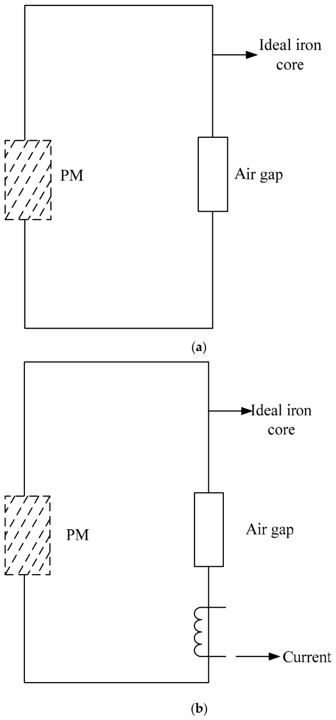
The calculation of the working point of PMs includes the calculation of no-load, rated load, and maximum demagnetization point. During the operation of the PMSM, the working point of the PM changes. When the IPMSM is in different working states, the magnetic circuit of the PM is different. The schematic diagram of the magnetic circuit of the PM under different operating states is shown in Figure 18. The IPMSM studied in this paper is a speed-regulating IPMSM. When the stator winding suddenly experiences a short circuit, the PM is prone to demagnetization. When a short-circuit fault occurs, a large short-circuit current will be generated in stator winding, with a large proportion of the direct-axis component. When the demagnetization field generated by the direct-axis current component reaches a certain degree, the PM will undergo irreversible demagnetization.

The critical demagnetization current for a speed-regulating IPMSM in the event of a short-circuit fault is approximately:

$$I_h\approx {\displaystyle \frac{E_0}{X_d}}$$

(34)

5.3. Analysis of Demagnetization of PMs Considering Temperature and Short-Circuit Current

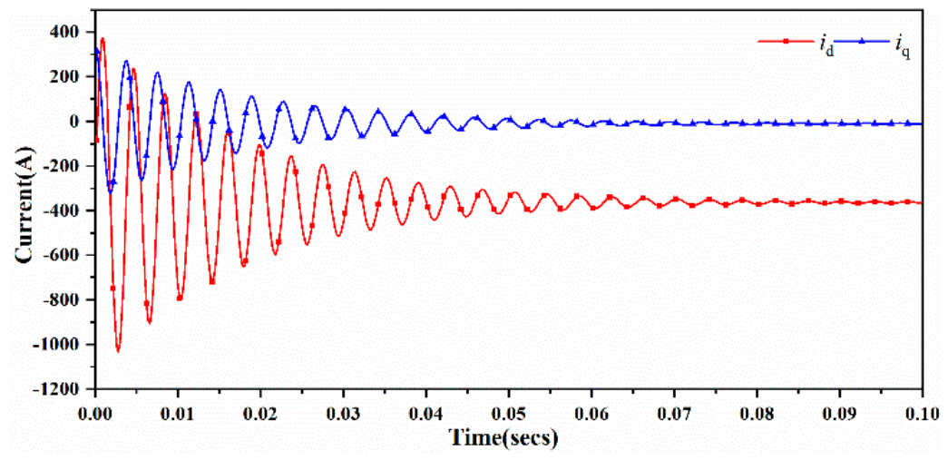
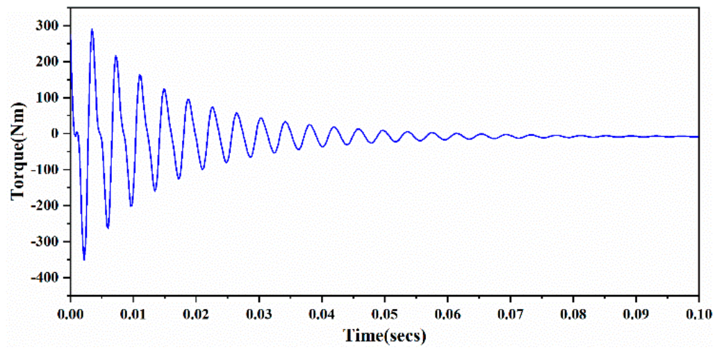
To analyze and study the demagnetization characteristics of PMs, it is necessary to densify the mesh of PMs. The demagnetization of NdFeB generally occurs at high temperatures. The temperature of the PM is 160 °C, the amplitude of the peak current is 480 A, and the current angle θ is 135°. The torque change curve during a sudden short circuit is shown in Figure 19, and the corresponding d–q short-circuit currents i_d and i_q are shown in Figure 20. From Figure 19, it can be seen that under the short-circuit condition, the output torque rapidly decreases to 0 Nm. From Figure 20, it can be seen that the d-axis peak current value corresponding to a sudden short circuit is 1000 A.

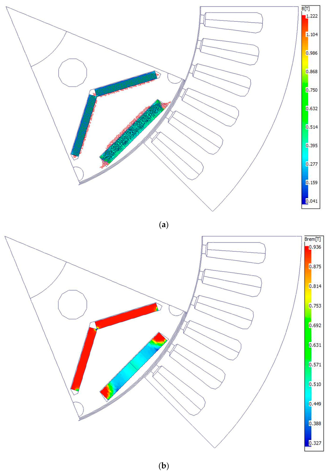
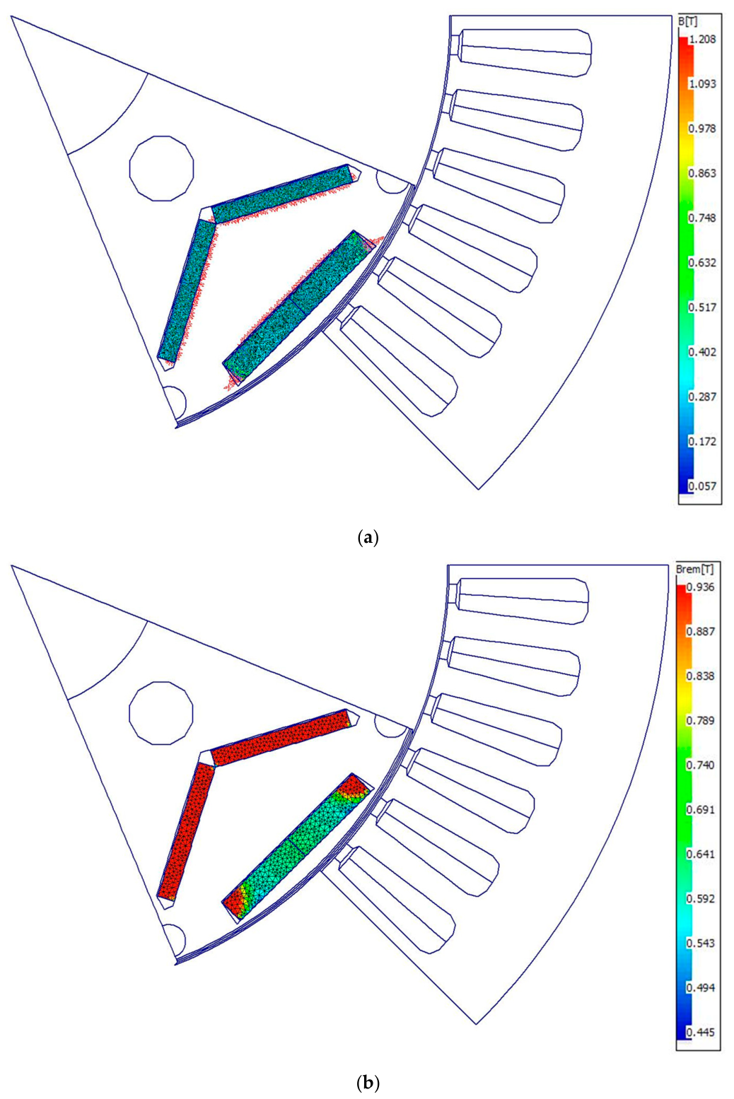
Under the condition of a current amplitude of 1000 A and a current control angle θ of 180°, the flux density cloud map of the demagnetized PM obtained by FEA of the demagnetization model is shown in Figure 21. From Figure 21, it can be seen that the first layer of V-type PMs has almost no demagnetization, and the magnetization direction remains basically unchanged, with a very small demagnetization rate of about 2.6%. The second layer of I-type PMs has severe demagnetization, and the magnetization direction has basically reversed, with a demagnetization rate of about 86.3%.

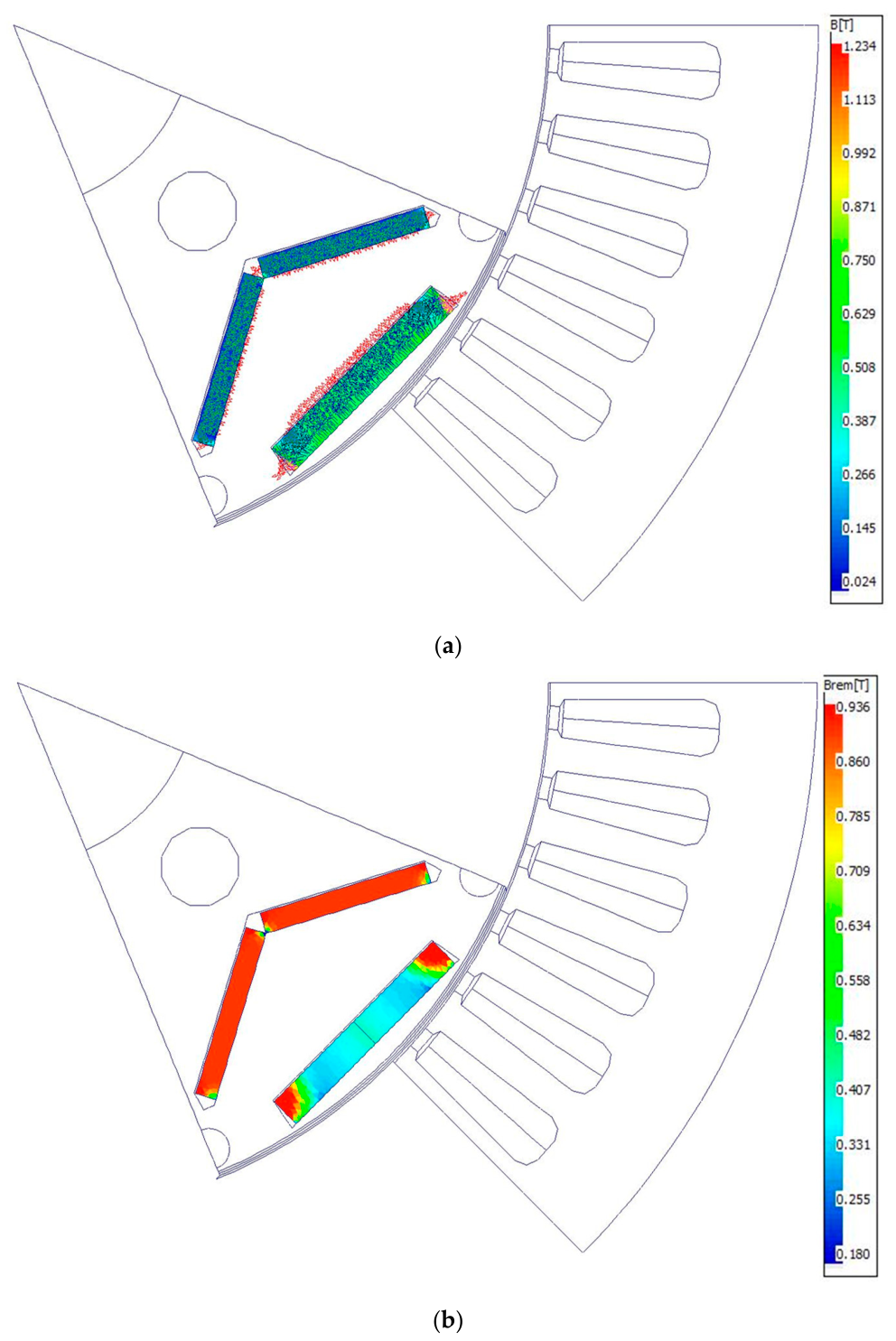
Keeping the current angle constant and increasing the current amplitude to 1250 A, the finite element solution of demagnetization model obtained flux density cloud after demagnetization, as shown in Figure 22. From Figure 22, it can be seen that the first layer of V-type PMs has relatively severe demagnetization, and the demagnetization rate is about 91.5%. The second layer of I-type PMs also has severe demagnetization, with a demagnetization rate of about 90.0%. The total demagnetization rate of the two layers of PMs is 91.1%.

The flux density cloud map of demagnetized PMs obtained when the current angle remains constant and the current amplitude increases to 1500 A is shown in Figure 23. From Figure 23, it can be seen that the first layer of the V-type PM has severe demagnetization, with a demagnetization rate of about 99.2%. The second layer of the I-type PM also has severe demagnetization, with a demagnetization rate of about 90.5%.

5.4. Comparison of Torque Before and After Demagnetization

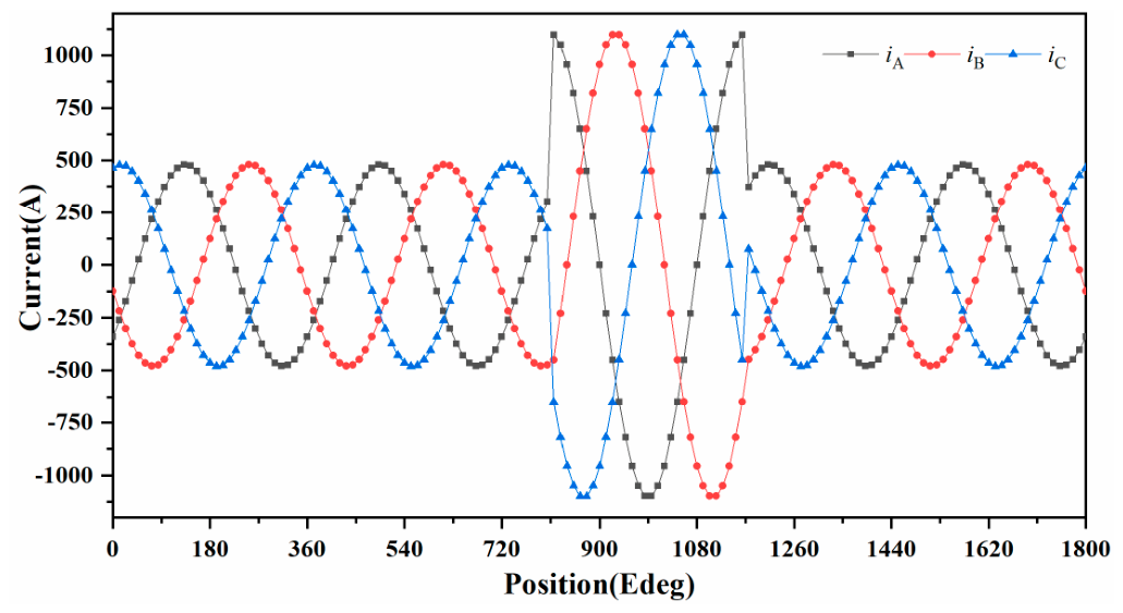
Under the working conditions of peak current amplitude of 480 A, current control angle θ of 180°, and PM temperature of 160 °C, the driving current waveform simulating a sudden short circuit of the IPMSM is shown in Figure 24. The driving current is five cycles, and a sudden short circuit occurs in the third driving cycle.

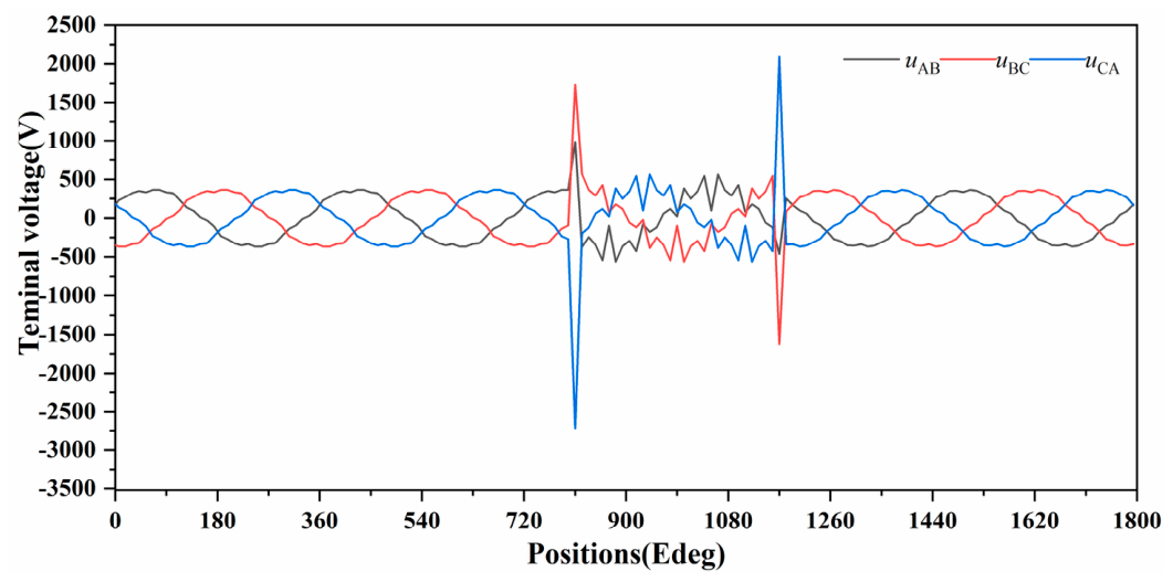
Solving the electromagnetic model, the terminal voltage distribution of the IPMSM can be obtained, as shown in Figure 25. From Figure 25, it can be seen that when the IPMSM experiences a short circuit in the third driving cycle, the waveform of the terminal voltage of the IPMSM has undergone severe distortion.

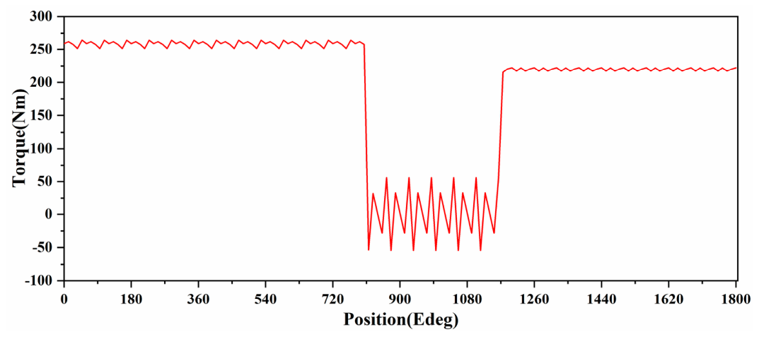
After a short circuit occurred in the third driving cycle, the IPMSM experienced irreversible demagnetization. The comparison of peak output torque before and after demagnetization is shown in Figure 26. Under normal circumstances, no short-circuit demagnetization occurred, and the peak torque of the IPMSM was 257.6 Nm. When a short circuit occurred in the third driving cycle, the output torque dropped suddenly to 0 Nm. After the short-circuit state ended, due to irreversible demagnetization of the IPMSM, the peak output torque decreased. After demagnetization, the average peak output torque decreased to 220 Nm, and the peak output torque decreased by 37.6 Nm, a decrease of 14.6%.

5.5. Comparison of No-Load Back EMF Before and After Demagnetization

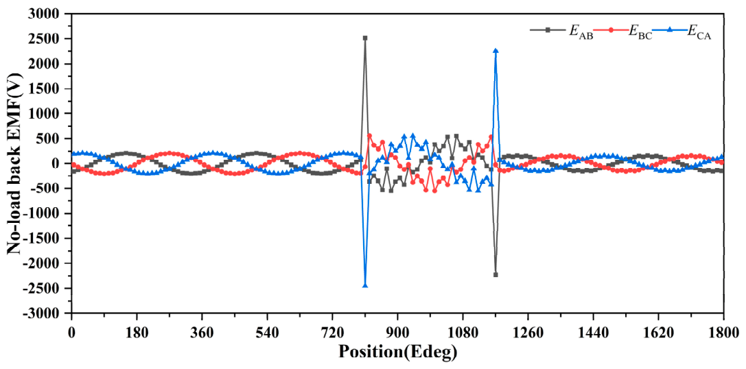
The waveform of no-load line back EMF as the IPMSM has a sudden short-circuit is shown in Figure 27. From Figure 27, it can be seen that when a short circuit occurs in the third driving cycle, the waveform distortion of the no-load line back EMF is severe.

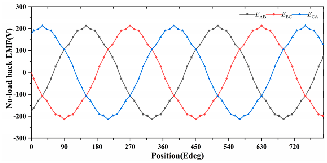
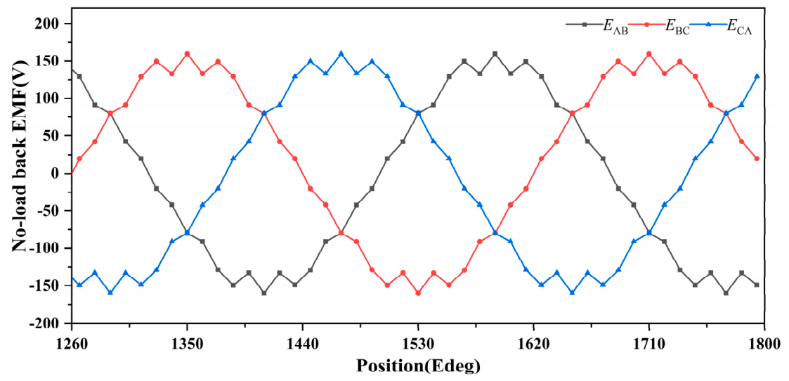
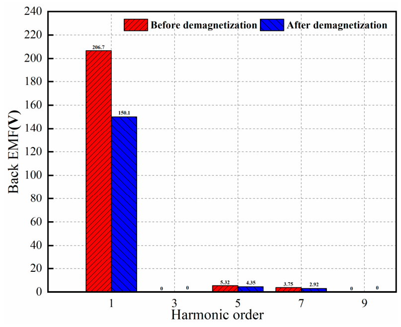
The waveforms of no-load line back EMF before and after demagnetization are shown in Figure 28 and Figure 29, respectively. From Figure 28, it can be clearly seen that the waveform of back EMF before demagnetization has a high sine degree, with a low harmonic distortion rate. The amplitude of no-load line back EMF is about 213.5 V. The amplitude of no-load line back EMF after demagnetization is about 159.7 V, and after irreversible demagnetization, the amplitude of no-load line back EMF decreases by 53.8 V, a decrease of about 25.2%. Comparing Figure 28 and Figure 29, it is found that after demagnetization, the amplitude of no-load line back EMF not only decreases significantly, but also the harmonic distortion rate of waveform further increases.

The comparison of harmonic distribution of no-load back EMF before and after demagnetization can be obtained from Figure 28 and Figure 29, as shown in Figure 30. The fundamental value of no-load line back EMF and the total harmonic distortion rate (THD) can be obtained from Figure 30, as shown in

Table 7. Amplitude of the fundamental and THD of no-load back EMF before and after demagnetization.

Parameters	Before Demagnetization	After Demagnetization
Fundamental amplitude of back EMF (V)	206.7	150.1
THD (%)	2.53	3.48

. From Table 7, it can be seen that the fundamental amplitude of the no-load line back EMF before demagnetization is 206.7 V, and the THD is 2.53%. After demagnetization, the fundamental amplitude of the no-load line back EMF decreased to 150.1 V, and the THD was 3.48%. Compared with before demagnetization, the fundamental amplitude decreased by 27.4%, and the THD increased by 37.5%.

6. Conclusions

IPMSMs have advantages of high power density and large output torque, but there is a risk of demagnetization in PMs. Currently, determining whether PMs undergo irreversible demagnetization mainly relies on the relationship between the working point of PMs and the knee point of the demagnetization curve. This paper takes an IPMSM with 48 slots, 8 poles, and 66 kW as the research object and studies the demagnetization of the PM under uniform demagnetization, local demagnetization, and stator winding with different demagnetization currents. The magnetic properties of PM materials were described based on various characteristic curves, and the reasons for the irreversible demagnetization of PMs were analyzed. Combined with the demagnetization reasons, the process of the irreversible demagnetization of PMs was studied. A two-dimensional simulation model of an IPMSM was built, and the stator winding resistance, no-load back EMF, and flux linkage of the PM were calculated at different temperatures. The values of d–q-axis inductance and torque performance were analyzed at different currents. We analyzed demagnetization curves of N30UH at different temperatures, and based on whether the minimum operating point of the PM is lower than the knee point of the demagnetization curve, we obtained the basic basis for the irreversible demagnetization of PMs.

By using finite element simulation software, a uniform demagnetization model as a whole and a local demagnetization model for PMs were built. The variation laws of performance parameters with output torque and no-load back EMF were analyzed. It was found that as the PM undergoes irreversible demagnetization, the amplitude no-load line back EMF and output torque decreased. The average peak output torque decreased to 220 Nm, a decrease of 37.6 Nm, or 14.6%. The fundamental amplitude of the no-load line back EMF before demagnetization is 206.7 V, and the THD is 2.53%. After demagnetization, the fundamental amplitude of the no-load line back EMF decreased to 150.1 V, and the THD was 3.48%. Compared with before demagnetization, the fundamental amplitude decreased by 27.4%, and the THD increased by 37.5%.

Based on the existing achievements of this study, further research and extension will be carried out in the following aspects in the future: optimizing the rotor topology structure, combining new topology design concepts, and continuously improving the anti-demagnetization performance and energy conversion efficiency of IPMSMs; exploring the adaptability of new high-performance permanent magnet materials in this design scheme, verifying the improvement effect of the new materials on the anti-demagnetization ability and comprehensive performance of IPMSM; promoting the construction of a prototype processing and testing platform, verifying the accuracy of simulation conclusions through physical testing, and further improving the practicality and credibility of research results. At the same time, the research scope will be extended to complex extreme working conditions, such as high- and low-temperature environments, frequent start–stop, overload impact, etc., systematically improving the variation patterns of the performance of motors under different operating conditions and providing reference and guidance for subsequent research in related fields. It should be noted that this study is limited to the simulation analysis of a single motor and a single magnet grade, so the research conclusions have certain limitations in universality. In future research, we will carry out comparative tests on multiple magnet grades and conduct physical prototype experiments for verification, so as to further revise and improve the research conclusions and enhance their applicability in engineering practice.

References

1. Ding, H.C.; Liu, L.W.; Nan, L. Calculation and Analysis of air gap flux density for surface permanent magnet synchronous motor. Comput. Simul. 2018, 35, 179–183. [Google Scholar]
2. Liu, G.H.; Wang, Y.Y. Multi-objective optimization of an symmetric V-shaped interior permanent magnet synchronous motor. Trans. China Electrotech. Soc. 2018, 33, 385–393. [Google Scholar]
3. Zhou, P.; Lin, D.; Xiao, Y. Temperature-dependent Demagnetization model of permanent magnets for finite element analysis. IEEE Trans. Magn. 2012, 48, 1031–1034. [Google Scholar] [CrossRef]
4. Klontz, K.W.; Miller, T.J.; McGilp, M.I.; Karmaker, H.; Zhong, P. Short-circuit analysis of permanent magnet generators. IEEE Trans. Ind. Appl. 2011, 47, 1670–1680. [Google Scholar] [CrossRef]
5. Chen, H.; Wang, X.; Wang, K. Demagnetization analysis of line-start permanent magnet synchronous motor with composite rotor under abnormal conditions. In IEEE Transportation Electrification Conference and Expo, Asia-Pacific (ITECAsia-Pacific); IEEE: New York, NY, USA, 2017; pp. 1–6. [Google Scholar]
6. Tang, X.; Wang, X.; Li, G.; Tian, M. Demagnetization study of line-start permanent magnet synchronous motor under out-of-step and super synchronous faults. In IEEE 11th Conference on Industrial Electronics and Applications (ICIEA); IEEE: New York, NY, USA, 2016; pp. 1496–1501. [Google Scholar]
7. Khan, M.S.; Okonkwo, U.V.; Usman, A.; Rajpurohit, B.S. Finite element modeling of demagnetization fault in permanent magnet direct current motors. In IEEE Power & Energy Society General Meeting (PESGM); IEEE: New York, NY, USA, 2018; pp. 1–5. [Google Scholar]
8. Hwang, K.Y.; Rhee, S.B.; Lee, J.S. Shape optimization of rotor pole in spoke type perm-anent magnet motor for reducing partial demagnetization effect and cogging torque. In International Conference on Electrical Machines and Systems (ICEMS); IEEE: New York, NY, USA, 2007; pp. 955–960. [Google Scholar]
9. Kim, K.C.; Kim, K.; Lee, J.S. Demagnetization analysis of permanent magnets according to rotor types of interior permanent magnet synchronous motor. IEEE Trans. Magn. 2009, 45, 2799–2802. [Google Scholar] [CrossRef]
10. Takahashi, N.; Shinagawa, H.; Miyagi, D.; Doi, Y.; Miyata, K. Analysis of eddy current losses of segmented NdFeB sintered magnets considering contact resistance. IEEE Trans. Magn. 2009, 45, 1234–1237. [Google Scholar] [CrossRef]
11. Zhao, G.; Tian, L.; Shen, Q.; Tang, R. Demagnetization analysis of permanent magnet synchronous machines under short circuit fault. In IEEE Asia-Pacific Power and Energy Engineering Conference; IEEE: New York, NY, USA, 2010; pp. 1–4. [Google Scholar]
12. Usman, A.; Rajpurohit, B.S. Characteristic analysis of partial demagnetization faults in surface mounted BLDC motors. In IEEE Industry Applications Society Annual Meeting; IEEE: New York, NY, USA, 2020; pp. 1–8. [Google Scholar]
13. Ruoho, S.; Dlala, E.; Arkkio, A. Comparison of demagnetization models for finite-element analysis of permanent magnet synchronous machines. IEEE Trans. Magn. 2007, 43, 3964–3968. [Google Scholar] [CrossRef]
14. Hamidizadeh, S.; Alatawneh, N.; Chromik, R.R.; Lowther, D.A. Comparison of different demagnetization models of permanent magnet in machines for electric vehicle application. IEEE Trans. Magn. 2016, 52, 2100304. [Google Scholar] [CrossRef]
15. Baranski, M.; Szelag, W.; Lyskawinski, W. Experimental and simulation studies of partial demagnetization process of permanent magnets in electric motors. IEEE Trans. Energy Convers. 2021, 36, 3137–3145. [Google Scholar] [CrossRef]
16. McFarland, J.D.; Jahns, T.M. Investigation of the rotor demagnetization characteristics of interior PM synchronous machines during fault conditions. IEEE Trans. Ind. Appl. 2013, 50, 2768–2775. [Google Scholar] [CrossRef]
17. Kim, K.C.; Lim, S.B.; Koo, D.H.; Lee, J. The shape design of permanent magnet for permanent magnet synchronous motor considering partial demagnetization. IEEE Trans. Magn. 2006, 42, 3485–3487. [Google Scholar] [CrossRef]
18. Kang, J.K.; Hur, J. Fault mechanism analysis of irreversible demagnetization due to the dynamic eccentricity of IPMSM for EV traction. IEEE Access 2022, 10, 64483–64494. [Google Scholar] [CrossRef]
19. Tang, Y.; Sun, S.; Yu, W.; Hua, W. Thermal analysis of water-cooling permanent magnet synchronous machine for port traction electric vehicle. Electronics 2023, 12, 734. [Google Scholar] [CrossRef]
20. Ge, S.; Zhao, J.; Wang, H.; Zhang, Z.; Qi, W. Electromagnetic thermal coupling characteristics of permanent magnet synchronous motor for electric vehicles. Proc. Inst. Mech. Eng. Part D J. Automob. Eng. 2025, 239, 6065–6083. [Google Scholar]
21. Yang, Y.J.; Kim, D.H.; You, Y.M. Demagnetization analysis of interior permanent magnet synchronous motors under realistic vehicle driving conditions. IEEE Access 2026, 14, 6501–6513. [Google Scholar] [CrossRef]
22. Sugimoto, S. Towards high coercivity Dy-free Nd-Fe-B sintered magnets. In Proceedings of the 20th International Workshop on Rare-Earth Permanent Magnet & Their Applications, Crete, Greece, 8–10 September 2008; pp. 106–110. [Google Scholar]
23. Liu, Z.; Zhou, B.; Liao, X.; He, J. Research status and future development of (Ce, La, Y)-Fe-B permanent magnets based on full high-abundance rare earth elements. Acta Met. Sin 2024, 60, 585–604. [Google Scholar]
24. Matsuura, Y. Recent development of Nd–Fe–B sintered magnets and their applications. J. Magn. Magn. Mater. 2006, 303, 344–347. [Google Scholar] [CrossRef]
25. Le, Z.Y. Numerical Simulation of the Demagnetization of a permanent magnet retarder in high temperature. Int. J. Plant Eng. Manag. 2009, 14, 238–242. [Google Scholar]
26. Jie, L.; Ke, X.; Nisoli, C. Local studies of AC demagnetization in a model frustrated magnet. In Proceedings of the APS March Meeting, New Orleans, LA, USA, 10–14 March 2008. [Google Scholar]
27. Ruoho, S.; Kolehmainen, J.; Ikaheimo, J. Interdependence of demagnetization, loading, and temperature rise in a permanent-magnet synchronous motor. IEEE Trans. Magn. 2010, 46, 949–953. [Google Scholar] [CrossRef]
28. Baranski, M.; Szelag, W.; Jedryczka, C. Influence of temperature on partial demagnetization of the permanent magnets during starting process of line start permanent magnet synchronous motor. In International Symposium on Electrical Machines (SME); IEEE: New York, NY, USA, 2017; pp. 1–6. [Google Scholar]
Figure 1. PM hysteresis loop.
Wevj 17 00299 g001
Figure 2. Recovery line of PM material.
Wevj 17 00299 g002
Figure 3. Knee point of PM material.
Wevj 17 00299 g003
Figure 4. Relationship between demagnetization curve and intrinsic demagnetization curve.
Wevj 17 00299 g004
Figure 5. Process diagram for demagnetization of PMs.
Wevj 17 00299 g005
Figure 6. Relationship between d–q-axis inductance and current.
Wevj 17 00299 g006
Figure 7. Phasor diagram of IPMSM in d–q coordinate system.
Wevj 17 00299 g007
Figure 8. Calculation curve of torque angle characteristic.
Wevj 17 00299 g008
Figure 9. Torque versus current angle under rated conditions.
Wevj 17 00299 g009
Figure 10. Torque distribution. (a) Electromagnetic torque. (b) Cogging torque.
Wevj 17 00299 g010
Figure 11. Influence of winding temperature on motor performance.
Wevj 17 00299 g011
Figure 12. Influence of PM temperature on electromagnetic performance. (a) Influence of temperature rise on air gap flux density and torque. (b) Influence of temperature rise on residual flux density and iron loss.
Wevj 17 00299 g012aWevj 17 00299 g012b
Figure 13. Schematic diagram of electromagnetic–thermal coupling.
Wevj 17 00299 g013
Figure 14. Flow chart for temperature rise calculation of IPMSM.
Wevj 17 00299 g014
Figure 15. Temperature comparison of motor. (a) Average temperature of winding. (b) Average temperature of PM.
Wevj 17 00299 g015aWevj 17 00299 g015b
Figure 16. Comparison of electromagnetic performance. (a) Average torque. (b) Output power. (c) Copper loss. (d) Iron loss.
Wevj 17 00299 g016aWevj 17 00299 g016b
Figure 17. Intrinsic demagnetization and demagnetization curve of N30UH.
Wevj 17 00299 g017
Figure 18. Magnetic circuit of PM. (a) No-load operation. (b) Load operation.
Wevj 17 00299 g018
Figure 19. Torque variation curve during short circuit.
Wevj 17 00299 g019
Figure 20. d–q current variation curve under short circuit.
Wevj 17 00299 g020
Figure 21. Flux density cloud map with 1000 A. (a) Demagnetization cloud map. (b) Remanent magnetism cloud map.
Wevj 17 00299 g021
Figure 22. Flux density cloud map with 1250 A. (a) Demagnetization cloud map. (b) Remanent magnetism cloud map.
Wevj 17 00299 g022
Figure 23. Flux density cloud map with 1500 A. (a) Demagnetization cloud map. (b) Remanent magnetism cloud map.
Wevj 17 00299 g023
Figure 24. Waveform of driving current.
Wevj 17 00299 g024
Figure 25. Waveform of terminal voltage.
Wevj 17 00299 g025
Figure 26. Comparison of torque before and after demagnetization.
Wevj 17 00299 g026
Figure 27. Waveform of no-load line back EMF during short circuit.
Wevj 17 00299 g027
Figure 28. Waveform of no-load line back EMF before demagnetization.
Wevj 17 00299 g028
Figure 29. Waveform of no-load line back EMF after demagnetization.
Wevj 17 00299 g029
Figure 30. Comparison of harmonic distribution of no-load line back EMF before and after demagnetization.
Wevj 17 00299 g030