Demand Response Equilibrium and Congestion Mitigation Strategy for Electric Vehicle Charging Stations in Grid–Road Coupled Systems

Abstract

With the increasing adoption of electric vehicles (EV), congestion at charging stations during peak hours has become a prominent issue, imposing significant pressure on station scheduling. Furthermore, the large-scale integration of photovoltaics (PV) introduces dual uncertainties in both generation and load, negatively impacting grid voltage. To tackle the above problems, a strategy for demand response balancing and congestion alleviation of charging stations under grid–road network partition mapping is proposed in this paper. Firstly, a user demand response capability assessment method based on the Fogg Behavior Model is proposed to evaluate the demand response potential of individual users in each zone. The results are aggregated to obtain the demand response participation capability of each zone, thereby realizing capability-based allocation and achieving demand response balancing. Secondly, the road network is divided into several zones and mapped to the power grid, and a two-layer cross-zone collaborative autonomy model is established. The upper layer aims to alleviate inter-zone congestion and balance inter-station power, taking into account the grid voltage level. A tripartite benefit model involving the power grid, charging stations and users is constructed, and an inter-zone mutual-aid model for the upper layer is established and solved optimally. The lower layer establishes an intra-zone self-consistency model, which subdivides different functional zone types within the road network zone, allocates and accommodates the cross-zone power from the upper-layer output inside the zone, and synchronously performs intra-zone cross-zone judgment to avoid congestion at charging stations. Simulation verification is carried out on the IEEE 33-bus system. The results show that the proposed method can effectively alleviate the congestion of charging stations, the balance degree among all zones is increased by 43.58%, and the power grid voltage quality is improved by about 38%. This study offers feasible guidance for exploring large-scale planned participation of electric vehicles in power system demand response.

1. Introduction

The widespread development of EV has brought about challenges, especially the excessive congestion during peak charging demand periods, which imposes enormous pressure on both charging facilities and power systems [1,2]. The National Development and Reform Commission and other relevant authorities jointly issued the Three-Year Doubling Action Plan for the Service Capacity of Electric Vehicle Charging Facilities (2025–2027), aiming to construct 28 million charging facilities by the end of 2027 [3]. Meanwhile, to fulfill the “dual carbon” goals [4], the installed capacity of PV is expanding progressively. However, the large-scale grid connection of PV systems introduces unpredictable intermittent power generation, leading to grid voltage violations that cannot be effectively mitigated by existing voltage regulation strategies alone [5,6,7]. Given the problems of EV charging station congestion, unbalanced charging loads among stations, and the increasingly severe issue of grid voltage violations, the integration of high-penetration PV and EV systems has become a key solution. This integration can simultaneously address charging station congestion, balance inter-station charging loads, and regulate grid voltage.

Regarding the quantification of user participation in demand response, ref. [8] constructs an EV grid-responsive model under a market environment, considering multiple market mechanisms. Reference [9] proposes a multi-time-scale optimal dispatching strategy for EV aggregators considering the reliability of EV peak-shaving demand response, and adopts a reservation mechanism to handle the uncertainties caused by EVs. In [10], a power allocation model is built with the goal of satisfying users’ travel demands to guide EVs to participate in system dispatching in an orderly manner. Ref. [11] develops a quantitative evaluation model of user response willingness considering the impact of multiple parameters, and sets parameters based on quantitative results to further improve users’ response willingness. Ref. [12] considers the randomness of vehicle arrival and parking times, as well as various preferences and demands of drivers. Similarly, ref. [13] considers the potential environmental fluctuation factors of EVs and introduces a decentralized operation paradigm for real-time EV dispatching, fully accounting for the subjective uncertainties of users.

In summary, although existing studies have explored EV demand response from different perspectives, such as market mechanisms, scheduling strategies, and user willingness, they generally lack systematic behavioral theory support, the characterization of users’ subjective and objective behavioral factors is incomplete, and the uncertainty modeling methods are relatively simplified. Furthermore, few studies investigate the schedulability of user participation in demand response to mitigate the negative impacts of user response uncertainty, which makes it difficult to fully support accurate and robust scheduling decisions in practical scenarios.

In the research field of EV functional zone division and zonal dispatching, ref. [14] proposes a two-layer optimal dispatching model for flexible resources in distribution networks, considering dynamic EV congestion, aiming to solve charging and discharging congestion and regulate spatiotemporal flexible resources. Ref. [15] minimizes the charging costs of EV users and maximizes the profits of EV aggregators by formulating free electricity prices and cooperative electricity prices, while promoting the consumption of distributed PV. In [16], a multi-objective EV dispatching model is proposed that fully considers the optimal economic trade-off among EV owners, charging stations, and the power grid. Ref. [17] designs a dynamic pricing mechanism to balance the interests of all parties in the integrated energy system. Ref. [18] first takes the maximization of the total profits of aggregators and EV users as the objective based on the peak-shaving demand of each time period, and then optimizes the charging and discharging strategies of subsequent periods with the goal of minimizing load fluctuations to avoid load spikes. Ref. [19] proposes a dispatching framework including EV, charging stations, and the power grid, which further promotes EV to participate in demand response services and avoids station congestion.

In summary, although existing studies have explored electric vehicle scheduling around the interests of the power grid, charging stations and users, they generally suffer from unbalanced multi-stakeholder objective setting, insufficient consideration of the comprehensive advantages brought by regional coordination, and a lack of attention to charging station congestion control and response balance among stations. As a result, the proposed scheduling strategies are difficult to adapt to the requirements of practical and complex scheduling scenarios.

In terms of the zoning coordination mechanism, ref. [20] proposes a distributionally robust joint chance-constrained dispatching model for EV–distribution network charging and discharging, which allocates charging and discharging demands to individual stations in real time. Ref. [21] establishes a dynamic grouping-based EV cluster dispatching model, which reduces grid load fluctuations while satisfying the individual charging demands of EVs. In [22], the coordination of multi-stakeholder interests in complex, uncertain environments is realized by formulating risk-aware, responsive electricity prices and evaluating the charging and discharging behaviors of EV users. Ref. [23] puts forward a novel transmission and distribution network dispatching model considering EV penetration rates across different time scales, whereas [24] constructs an EV cluster model to effectively manage the charging and discharging of EV clusters and allocate resources to each node. This line of research is further enhanced by an adjustable capacity decision-making model for EV proposed in [25], which further considers the characteristics of EV in different functional zones and realizes flexible aggregation and smooth control of EV.

In summary, most existing studies only conduct coordinated control for the same type of region or a single functional area, and have not yet uniformly divided multi-type functional area clusters into zones. Such methods only achieve scheduling optimization among different regions, but ignore the collaborative interaction and coupling impact among different functional areas within a region, making it difficult to accurately characterize the spatiotemporal coupling characteristics of traffic travel distribution and power grid load, resulting in poor applicability of the scheduling strategy.

Overall, based on the research of previous studies, this paper proposes a user demand response potential evaluation method based on the Fogg Behavior Model and constructs the Two-Layer Cross-Regional Collaborative–Autonomous Model, aiming to make up for the shortcomings of existing research and improve the scientificity of scheduling strategies. The main innovations are as follows:

• A response potential evaluation method integrating the Fogg Behavior Model is proposed. By constructing a multi-dimensional evaluation system including the response ability, motivation, and triggers of EV owners, the demand response potential of charging stations in each zone is quantified, which matches the user response potential with the scheduling results, thereby promoting the balance of inter-station responses.
• An upper-layer inter-zone mutual assistance model is established. Focusing on the demand response balance and congestion alleviation of charging stations, various inter-zone operation scenarios are constructed through the mapping relationship between power grid nodes and road network zones. The cross-zone scheduling volume of charging stations, cross-zone incentive mechanisms and user demand response potential are incorporated into the objective function. Meanwhile, the voltage security of the power grid and the cost–benefits of the three parties are taken into account. Finally, the model is solved by an optimization algorithm.
• A lower-layer intra-zone self-consistency model is established. Various functional zones are further subdivided within the road network zone. With the core objective of preventing congestion at charging stations in sub-zones, the inter-zone power transmission quantities output by the upper-layer model are reasonably allocated and absorbed within the zone by introducing a relaxed congestion threshold and a delayed charging mechanism. Meanwhile, a cross-sub-zone mechanism is introduced within the sub-zones, further preventing congestion at charging stations.

This study is structured as follows: Section 2 introduces the EV load simulation method based on trip chains. Section 3 describes the modeling of each component in the power grid and road network coupled system. Section 4 proposes a bi-level cross-regional coordination and self-consistent model. Following this, Section 5 carries out simulations and analyzes the results. Finally, Section 6 presents the conclusion of the study.

2. EV Charging Load Simulation

In this paper, the functional zones of the road network are divided into residential areas, work areas, and leisure areas. EV depart from residential areas and head for either work areas or leisure areas [26]. The initial and destination positions of vehicles follow a uniform distribution, the initial departure time and state of charge (SOC) conform to a normal distribution, and the parking duration at the destination obeys an extreme-value distribution [27].

Matrix D is used to describe the length of each road segment and the connection relationship between nodes in the road network. There are multiple driving routes from node i to node j, and the shortest path for vehicle travel is solved by the Dijkstra algorithm.

$$D=\left[\begin{array}{cccc}0& l_{12}& \mathrm{\dots }& l_{\mathrm{i}\mathrm{j}}\\ l_{21}& 0& l_{23}& l_{\inf }\\ \mathrm{\dots }& l_{32}& 0& l_{\inf }\\ l_{\mathrm{i}\mathrm{j}}& l_{\inf }& l_{\inf }& \mathrm{\dots }\end{array}\right]$$

(1)

where D denotes the road matrix; $l_{\mathrm{ij}}$ represents the actual length of the road segment between nodes i and j; and $l_{\inf }$ indicates no road connection between the road nodes.

Temperature exerts a significant impact on battery endurance, and the battery capacity decreases remarkably, especially at low temperatures, as shown in the following formula [28]:

$$C_T={\xi }_0+{\xi }_{1}T+{\xi }_2{T}^2+{\xi }_3{T}^3$$

(2)

where $C_T$ represents the relative capacity percentage of the battery at temperature T; ${\xi }_0$, ${\xi }_1$, ${\xi }_2$, ${\xi }_3$ are fitting coefficients; and T denotes temperature.

Vehicle speed directly affects energy consumption, and speed is mainly influenced by road traffic flow. To this end, an EV speed model is introduced to simulate vehicle driving speed, as shown in the following formula [29]:

$$\left\{\begin{array}{c}{v}_{ij,t}={\displaystyle \frac{v_{ij,t}}{1+{(\frac{q_{ij,t}}{c_{ij}})}^{\lambda }}}\\ \lambda =\alpha +\beta {({\displaystyle \frac{q_{ij,t}}{c_{ij}}})}^{\gamma }\end{array}\right.$$

(3)

where $v_{ij,t}$ denotes the free-flow speed of road segment ij at time t; i and j represent the road grade between the two locations; $q_{ij,t}$ is the traffic flow of road segment ij at time t; $c_{ij}$ denotes the capacity of road segment ij; and $\alpha$, $\beta$, $\gamma$ are adaptive factors.

We analyze the energy consumption of EVs during travel. Among all influencing factors, temperature and vehicle speed are the key ones affecting energy consumption. The model for EV energy consumption per unit mileage considering the impacts of temperature and vehicle speed is shown in the following formula [29]:

$$E_{t,n}={\displaystyle \frac{{\zeta }_1{v}_{ij,t}{\zeta }_2{\omega }_T}{C_T}}$$

(4)

where ${\zeta }_1$ and ${\zeta }_2$ are constant coefficients and ${\omega }_T$ is the temperature fitting parameter.

When a user is ready to travel, if the initial SOC fails to meet the mileage consumption requirement, charging will be conducted at the departure location to complete the trip. The SOC required for the user to reach the destination and the SOC variation model during the charging process are, respectively, as follows:

$$SO{C}_{\mathrm{c}\mathrm{ost},n}={\displaystyle \frac{L_{n,ij}{E}_{t,n}}{E_{\max }{C}_T}}$$

(5)

$$△SO{C}_{t,n}={\displaystyle \frac{{\eta }_{\mathrm{ch}}{p}_{\mathrm{e},\mathrm{ch}}^n△t}{E_{\max }{C}_T}}$$

(6)

where $SO{C}_{\mathrm{c}\mathrm{ost},n}$ denotes the total SOC required for the user to travel from the departure location to the destination; $△t$ represents a specific moment; $△SO{C}_{t,n}$ is the variation in the vehicle’s SOC over time $△t$; ${\eta }_{\mathrm{ch}}$ is the charging efficiency; $p_{\mathrm{e},\mathrm{ch}}^n$ is the rated charging power of the charging pile; and $E_{\max }$ is the rated capacity of the EV.

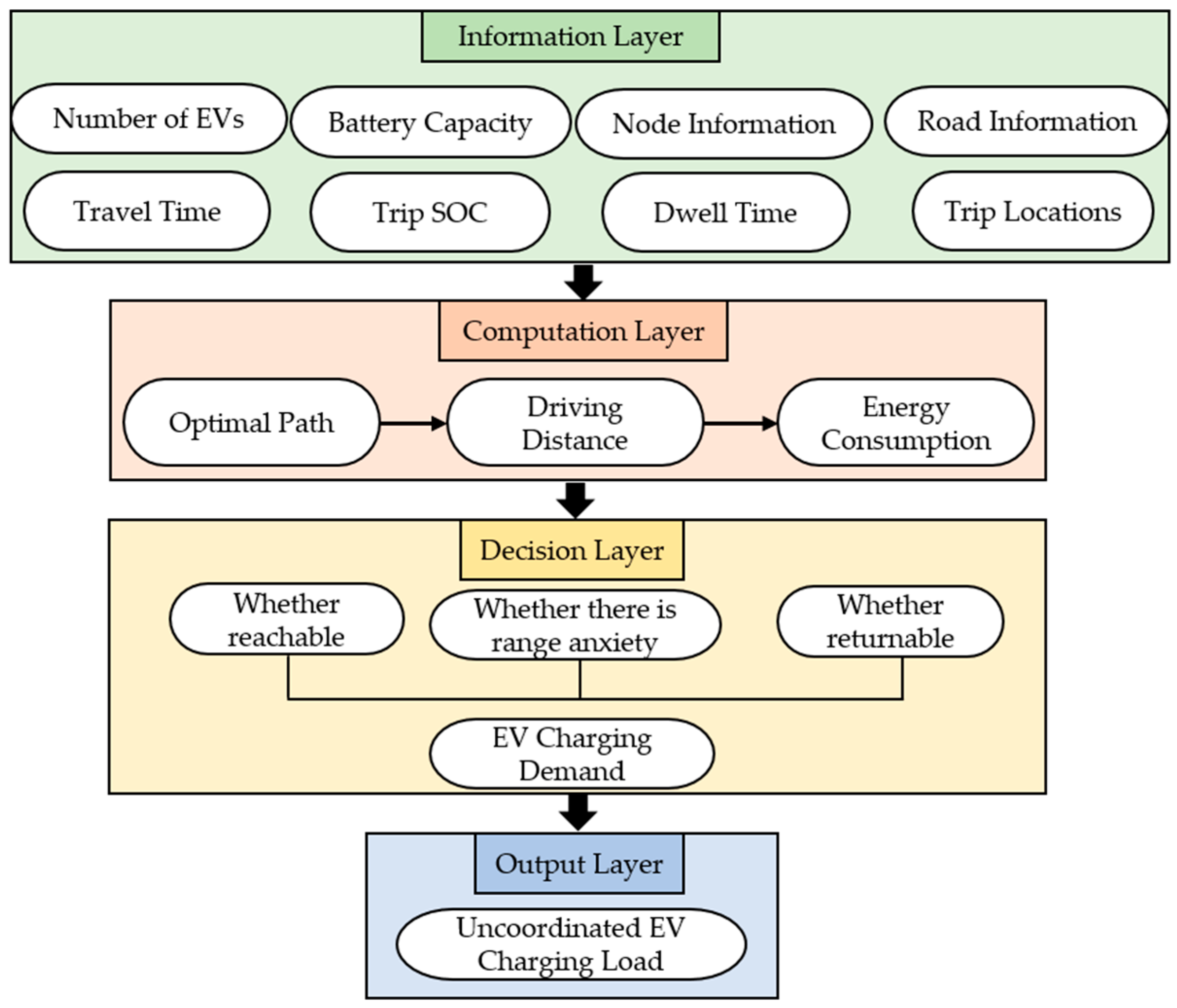
In summary, the main steps of electric vehicle load forecasting are illustrated in Figure 1, where different colors represent different levels respectively.

3. Grid–Road Network Coupling System Modeling

We construct an EV dispatching framework based on the grid–road network coupling system. Different zones are set on the road network, and each zone contains multiple sub-zones of different types, which are mapped to the power grid. On the user side, the Fogg Behavior Model is adopted to quantify each user’s potential to participate in demand response. Furthermore, on the charging station side, the demand response capacity of charging stations in each zone is obtained, which enhances the alignment between day-ahead dispatch results and users’ demand response potential. On the grid side, a floating-threshold band considering voltage margin is established to further avoid the impacts caused by various real-time uncertain factors during the day. Finally, a dynamic incentive mechanism between the power grid and charging stations is constructed to guide charging stations to actively participate in demand response. The system is modeled as follows.

3.1. User Modeling

When a vehicle arrives at a charging station and starts charging, based on the Monte Carlo prediction in Section 2, the SOC and remaining parking time of the vehicle during the charging process are updated as follows:

$$SO{C}_{t,n}^{\mathrm{sta}}=SO{C}_{\mathrm{in},\mathrm{evs}}+△SO{C}_{t,n}{T}_{\mathrm{cont}}$$

(7)

$$T_{t,n}^{\mathrm{sta}}=T_{stay,n}-t$$

(8)

where t represents time; $SO{C}_{t,n}^{\mathrm{sta}}$ and $T_{t,n}^{\mathrm{sta}}$ denote the remaining SOC and remaining parking time of the vehicle at time t, respectively; $SO{C}_{\mathrm{in},\mathrm{evs}}$ is the initial SOC of the vehicle when starting charging; and $T_{\mathrm{cont}}$ indicates the duration of charging.

The Fogg Behavior Model, a classic behavioral theory proposed by Professor B.J. Fogg from Stanford University, aims to explain the underlying logic of human behavior occurrence [30]. This model holds that the occurrence of a behavior requires three elements to be satisfied simultaneously: ability, motivation, and trigger, none of which can be absent. Based on this model, we quantitatively analyze users’ demand response potential according to the situation of grid voltage violations. The calibrated values of parameters in the following models are all obtained through MATLAB R2022b simulation modeling.

Based on the Fogg Model and the application scenario of this paper, the ability to perform the behavior is related to the vehicle’s SOC and remaining parking time, which is expressed by the Sigmoid function. The difference between the two lies in the fact that the SOC has an upper limit, while the remaining parking time has no upper limit; thus, a linear growth term is added to the function for the latter, as shown in the following formula:

$${\lambda }_{\mathrm{ev},t,n}=\left\{\begin{array}{c}{\displaystyle \frac{{\alpha }_{\mathrm{soc}}}{1+{\mathrm{e}}^{-k(SO{C}_{t,\mathrm{sta}}-\frac{SO{C}_{\max }}{2})}}}+{\displaystyle \frac{{\beta }_T{T}_{t,n}^{\mathrm{sta}}}{1+{\mathrm{e}}^{-k(SO{C}_{t,\mathrm{sta}}-SO{C}_{\max })}}},v_t<v_{\min }\\ {\displaystyle \frac{{\alpha }_{soc}}{1+{\mathrm{e}}^{-k[(1-SO{C}_{t,\mathrm{sta}})-\frac{SO{C}_{\max }}{2}]}}}+{\displaystyle \frac{{\beta }_T{T}_{t,n}^{sta}}{1+{\mathrm{e}}^{-k[(1-SO{C}_{t,\mathrm{sta}})-SO{C}_{\max }]}}},v_t>v_{\max }\end{array}\right.$$

(9)

where ${\lambda }_{\mathrm{ev},t,n}$ denotes the behavioral ability of vehicle n at time t; ${\alpha }_{\mathrm{soc}}$ and ${\beta }_T$ are response constant coefficients; $SO{C}_{\max }$ is the maximum value of SOC; $v_{\max }$ and $v_{\min }$ are the upper and lower limits of voltage, respectively; and $v_t$ denotes the day-ahead grid voltage at time t, which is obtained by power flow calculation based on the predicted EV load and PV output. The core formulae of power flow calculation are as follows:

$${\displaystyle \sum _{\mathrm{k}\in \mathsf{\delta }\left(\mathrm{j}\right)}{P}_{jk,t}}-{\displaystyle \sum _{i\in \pi \left(\mathrm{j}\right)}(P_{ij,t}-}{I}_{ij,t}^2{r}_{ij})=P_{j,t}^{pv}+P_{j,t}^{ev}+P_{j,t}^{load},\forall t,\forall j\in \Omega$$

(10)

$$V_{j,t}^2=V_{\mathrm{i},t}^2-2(P_{ij,t}{r}_{ij}+Q_{ij,t}{x}_{ij})+I_{ij,t}^2(r_{ij}^2+x_{ij}^2),\forall ij\in \Omega$$

(11)

$$I_{ij,t}^2={\displaystyle \frac{P_{ij,t}^2+Q_{ij,t}^2}{V_{ij,t}^2}},\forall t,\forall ij\in \Omega$$

(12)

where $P_{jk,t}$ is the active power flowing from node j to node k at time t; $P_{ij,t}$ is the active power flowing to node j from the node at time t; $P_{j,t}^{pv}$ is the PV output at node j at time t; $P_{j,t}^{\mathrm{e}v}$ is the EV load at node j at time t; $P_{j,t}^{\mathrm{load}}$ is the net load at node j at time t; $P_{ij,t}$ and $Q_{ij,t}$ are the active power and reactive power transmitted on line i-j at time t, respectively; $V_{\mathrm{i},\mathrm{t}}$ is the voltage at node i at time t; $I_{ij,t}$ is the current on line i-j at time t; $r_{ij}$ and $x_{ij}$ are the resistance and reactance on line i-j, respectively; $\mathsf{\delta }\left(\mathrm{j}\right)$ is the set of downstream nodes of node j; $\pi \left(\mathrm{j}\right)$ is the set of upstream nodes of node j; and $\Omega$ is the set of all nodes.

Users also need motivation to participate in demand response. Even with response capacity, it is difficult to trigger the behavior when motivation is insufficient. This model proposes that motivation is related to three factors, namely emotion, society, and environment, as shown in the following formula:

$${\epsilon }_{\mathrm{dr},t,n}^{\mathrm{ev}}=\left\{\begin{array}{c}({\alpha }_{\mathrm{ne},\mathrm{soc}}SO{C}_{t,n}^{\mathrm{sta}}+{\alpha }_{\mathrm{ne},\mathrm{T}}{T}_{t,n}^{\mathrm{sta}})+{\beta }_t^{\mathrm{env}}+{\gamma }_{\mathrm{soci}},v_t<v_{\min }\\ [{\alpha }_{\mathrm{ne},\mathrm{soc}}(1-SO{C}_{t,n}^{\mathrm{sta}})+{\alpha }_{\mathrm{ne},\mathrm{T}}{T}_{t,n}^{\mathrm{sta}}]+{\beta }_t^{\mathrm{env}}+{\gamma }_{\mathrm{soci}},v_t>v_{\max }\end{array}\right.$$

(13)

where ${\epsilon }_{\mathrm{dr},t,n}^{\mathrm{ev}}$ denotes the motivation of vehicle n to perform the behavior at time t; ${\alpha }_{\mathrm{ne},\mathrm{soc}}$ and ${\alpha }_{\mathrm{ne},\mathrm{T}}$ represent the user’s positive and negative emotional coefficients, respectively; ${\beta }_t^{\mathrm{env}}$ is a random environmental influencing factor and is set as a constant; and ${\gamma }_{\mathrm{soci}}$ is a social influencing factor related to the government policies and social customs of the region where the user is located, set as a constant.

Based on users’ response ability and motivation, a user’s demand response potential is derived and expressed by a behavioral coefficient, as shown in the following formula:

$$R_{t,n}^{\mathrm{ev}}={\lambda }_{\mathrm{ev},t,n}\mathrm{c}+(1-\mathrm{c}){\epsilon }_{\mathrm{dr},t,n}^{\mathrm{ev}}$$

(14)

where $R_{t,n}^{\mathrm{ev}}$ denotes the behavior coefficient of vehicle n at time t, and c is a constant.

Floating boundaries are dynamically divided to classify electric vehicles participating in demand response, thereby realizing the alignment between users’ participation willingness and grid dispatching needs, and further guiding the balanced allocation of response resources among charging stations in different zones. The division of floating boundaries for users’ participation in demand response depends not only on their own motivation and response ability, but also on the real-time operation needs of the power grid. To this end, a nonlinear mapping relationship is constructed based on grid voltage and users’ behavior coefficients, as shown in the following formula:

$$l_{\mathrm{ev},\lim }={\displaystyle \frac{{\displaystyle \sum _{n=1}^N{R}_{t,n}^{\mathrm{ev}}}}{N}}(a-e^{\mathrm{k}△v_t})$$

(15)

$$△v_t=\left|v_{\lim ,e}-v_t\right|$$

(16)

where $l_{\mathrm{ev},\lim }$ is the floating boundary; $△v_t$ denotes the degree of voltage violation at time t; $v_{\lim ,e}$ is the rated voltage of the power grid; N is the total number of EVs; a and k are constants.

Based on the floating boundaries, when a user’s own behavioral coefficient is greater than the trigger boundary, the trigger parameter ${\zeta }_{\mathrm{sw}}$ is set to 1 (indicating that the user is triggered to participate in demand response); otherwise, it is set to 0 (indicating that the user is not triggered). The number of vehicles triggered to participate in demand response in Zone Z at time t is as follows:

$$N_{\mathrm{dr},t,z}^{\mathrm{evs},\mathrm{refer}}={\displaystyle \sum _{n=1}^N{\zeta }_{\mathrm{sw}}}$$

(17)

where $N_{\mathrm{dr},t,z}^{\mathrm{evs},\mathrm{refer}}$ denotes the number of demand response vehicles in Zone Z at time t, and ${\zeta }_{\mathrm{sw}}$ is the trigger indicator parameter.

3.2. Power Station Modeling

According to Section 3.1, by evaluating the demand response potential of users with the Fogg Model, we obtain the number of vehicles triggered to participate in demand response within zone Z at time t, denoted as $N_{\mathrm{dr},t,z}^{\mathrm{evs},\mathrm{refer}}$. On this basis, the demand response capacity of the zone charging station is as follows:

$$P_{dr,t,z}^{evs,refer}=N_{dr,t,z}^{evs,refer}{P}_{e,v2g}$$

(18)

where $P_{dr,t,z}^{evs,refer}$ is the demand response capacity of Zone Z at time t; ${\zeta }_{\mathrm{sw}}$ is the demand response capacity of the charging station; and $P_{e,v2g}$ is the rated charging and discharging power of the charging station.

The formula for the charging station congestion degree is as follows:

$$D_{t,z}={\displaystyle \frac{N_{\mathrm{ch},t}}{N_{\max ,\mathrm{z}}^{\mathrm{evs}}}}$$

(19)

where $D_{t,z}$ is the congestion degree of Zone Z at time t; $N_{\mathrm{ch},t}$ is the number of vehicles being charged at the charging station at time t; and $N_{\max ,\mathrm{z}}^{\mathrm{evs}}$ is the capacity of the charging station.

3.3. Power Grid Modeling

In the analysis and modeling at the power grid level, the voltage floating-threshold band of the distribution network and the sensitivity judgment of power grid nodes are considered.

Considering the uncertainties of intra-day electric vehicle response and PV power prediction, a voltage floating-threshold band is set to reduce the impact of such uncertainties on system operation. The formula is given as follows:

$${\epsilon }_{\mathrm{v},t}={\delta }_{\mathrm{pv}}(△P_{t-1}^{\mathrm{dr}}+△P_{t+1}^{\mathrm{dr}})+{\delta }_{\mathrm{v}}{e}^{-v_t}$$

(20)

where ${\epsilon }_{\mathrm{v},t}$ is the voltage threshold margin at time t; ${\delta }_{\mathrm{pv}}$ and ${\delta }_{\mathrm{v}}$ represent margin coefficients; and $△P_{t-1}^{\mathrm{dr}}$ and $△P_{t+1}^{\mathrm{dr}}$ are the front and rear fluctuation differences in PV output at time t.

The upper and lower voltage limits, considering the margin, are obtained as follows:

$$V_{\min }=V_{\min }^{\mathrm{base}}+{\epsilon }_{\mathrm{v},t}$$

(21)

$$V_{\max }=V_{\max }^{\mathrm{base}}-{\epsilon }_{\mathrm{v},t}$$

(22)

where $V_{\min }$ and $V_{\max }$ are the lower and upper voltage limits, respectively, and $V_{\min }^{\mathrm{base}}$ and $V_{\max }^{\mathrm{base}}$ are the original lower and upper voltage limits.

The cross-zone judgment needs to consider the differences in voltage sensitivity of power grid nodes in different zones. For the same injected power, different node voltage sensitivities lead to different degrees of voltage variation. The node sensitivity matrix is given in [31]:

$$\left[\begin{array}{c}\Delta \theta \\ \Delta U\end{array}\right]=\left[\begin{array}{cc}{\displaystyle \frac{\partial \theta }{\partial P}}& {\displaystyle \frac{\partial \theta }{\partial Q}}\\ {\displaystyle \frac{\partial U}{\partial P}}& {\displaystyle \frac{\partial U}{\partial P}}\end{array}\right]\left[{\displaystyle \frac{\Delta P}{\Delta Q}}\right]$$

(23)

The node voltage sensitivity formula can be sorted out as follows:

$$A_Z=\Delta U={\displaystyle \frac{\partial U_Z}{\partial P_Z}}\Delta P_Z+{\displaystyle \frac{\partial U_Z}{\partial Q_Z}}\Delta Q_Z$$

(24)

where $A_Z$ is the voltage sensitivity of node z, and $\partial U_Z/\partial P_Z$ and $\partial U_Z/\partial Q_Z$ are the active and reactive power sensitivities of node z voltage, respectively.

3.4. Dynamic Incentive Modeling of Power Grid–Power Station

The power grid issues demand response incentives based on the degree of voltage violation. By introducing nonlinear dynamic incentives, it guides charging stations to actively participate in the response. When the voltage exceeds the upper limit, the power grid issues charging demands, and the incentive price for charging stations to purchase electricity is as follows:

$${\omega }_{\mathrm{price},\mathrm{ch},t}=\left\{\begin{array}{c}\exp [{\sigma }^{\mathrm{ch},\mathrm{ax}}(k^{\mathrm{ch}}-\Delta v_t)]{\omega }_{\mathrm{bs},t},\Delta v_t>{\beta }_{\mathrm{c}}\\ {\sigma }^{\mathrm{ch},\mathrm{in}}(v_{\max }-\Delta v_t){\omega }_{\mathrm{bs},t},\Delta v_t\le {\beta }_{\mathrm{c}}\end{array}\right.$$

(25)

where ${\omega }_{\mathrm{price},\mathrm{ch},t}$ is the grid charging incentive at time t; ${\sigma }^{\mathrm{ch},\mathrm{ax}}$ and ${\sigma }^{\mathrm{ch},\mathrm{in}}$ are charging incentive constants; ${\omega }_{\mathrm{bs},t}$ represents the basic time-of-use electricity price at time t; ${\beta }_{\mathrm{c}}$ denotes the voltage threshold; and $k^{\mathrm{ch}}$ is a constant.

When the voltage is below the lower limit, the power grid issues power generation demands, and the incentive price for charging stations to sell electricity is as follows:

$${\omega }_{\mathrm{price},\mathrm{dis},t}=\left\{\begin{array}{c}{\omega }_{\mathrm{bs},t}\ln [1+{\sigma }^{\mathrm{dis},\mathrm{ax}}(\Delta v_t-k^{\mathrm{dis}})],\Delta v_t>{\beta }_{\mathrm{c}}\\ {\sigma }^{\mathrm{dis},\mathrm{in}}\left(v_{\max }+\Delta v_t\right){\omega }_{\mathrm{bs},t},\Delta v_t\le {\beta }_{\mathrm{c}}\end{array}\right.$$

(26)

where ${\omega }_{\mathrm{price},\mathrm{dis},t}$ is the grid discharge incentive at time t; ${\sigma }^{\mathrm{dis},\mathrm{ax}}$ and ${\sigma }^{\mathrm{dis},\mathrm{in}}$ are discharge incentive constants; and $k^{\mathrm{dis}}$ is a constant.

4. Two-Layer Cross-Regional Collaborative–Autonomous Model

A two-layer cross-zone collaboration–autonomy model is constructed. The upper layer establishes an inter-zone mechanism among zones, classifies various inter-zone scenarios by integrating the different requirements of the power grid side and the charging station side, and guides each zone to realize mutual assistance dispatching. On this basis, the inter-zone interaction mechanism and the charging station demand response capacity calculated based on the Fogg Model are both included in the objective function. Meanwhile, the voltage quality of the power grid, as well as the costs and benefits of the grid side, charging station side, and user side are comprehensively considered, and the grid–charging station dynamic incentive is also included in the revenue objective of the optimization process. Corresponding constraints are established for the optimization variables in the objective function, and the voltage fluctuation threshold band is embedded into the grid voltage constraints. Finally, the optimal solution of the model is obtained. The lower layer distributes and absorbs the inter-zone volume obtained from the upper layer solution within each zone, and also carries out inter-zone judgment to avoid congestion at charging stations within the zone, so as to achieve accurate matching between the dispatching results and actual scenarios. The details are as follows.

4.1. Upper-Level Model

4.1.1. Upper-Level Cross-Regional Mechanism

At the upper layer, between zones, different cross-zone scenarios are set up, and cross-zone constraints, priorities, and incentives are established to alleviate congestion and regulate power grid voltage. Specifically, it is divided into the following scenarios.

Scenario 1: When charging stations are congested and power grid voltage violates limits, outgoing zones and receiving zones are selected based on congestion degree. A zone with a congestion degree greater than the threshold is regarded as an outgoing zone, and the remaining zones are receiving zones. The congestion degree threshold is represented by the average value of charging station congestion survey results in various regions [32], and the formula is as follows:

$$D_{\lim }={\displaystyle \frac{{\displaystyle \sum _{a=1}^{\mathrm{A}}{D}_a}}{A}}$$

(27)

where $D_{\lim }$ is the congestion degree threshold, and A is the set of various regions.

The minimum outgoing volume of an outgoing zone is the minimum value that ensures the outgoing zone can eliminate its own congestion. The maximum receiving volume of a receiving zone is the maximum value that ensures no congestion occurs during the receiving process. The formulae are as follows:

$$P_{t,z}^{\mathrm{need},\mathrm{step}}=(D_{t,z}-D_{\lim })P_{\mathrm{dr},t,z}^{\mathrm{evs},\mathrm{e}}$$

(28)

$$P_{t,z}^{\max ,\mathrm{carry}}=(D_{\lim }-D_{t,z})P_{\mathrm{dr},t,z}^{\mathrm{evs},\mathrm{e}}$$

(29)

where $P_{t,z}^{\mathrm{need},\mathrm{step}}$ and $P_{t,z}^{\max ,\mathrm{carry}}$ are the minimum outgoing volume of outgoing zone z and the maximum receiving volume of receiving zone z at time t, respectively.

If the total outgoing volume of a zone is excessively large, the receiving zone shall still accept it, and the excess part shall be handled by the lower layer of the receiving zone. The constraints for outgoing zones and receiving zones are as follows:

$$P_{t,z}^{\mathrm{need},\mathrm{step}}<P_{t,z}^{\mathrm{step}}<P_{t,z}^{\max ,\mathrm{step}}$$

(30)

$$0<P_{t,z}^{\mathrm{carry}}<P_{t,z}^{\max ,\mathrm{carry}}$$

(31)

where $P_{t,z}^{\max ,\mathrm{step}}$ denotes the maximum cross-zone volume of outgoing zone z at time t, which is equal to the sum of all charging powers in the station at time t.

Considering inter-zone and intra-zone factors, which are affected by cross-zone distance, node voltage sensitivity, and charging station congestion degree, the settings of outgoing priority and receiving priority are as follows:

$$F_{t,z}^{\mathrm{fs},\mathrm{step}}={\alpha }_{\mathrm{ste}}^{\mathrm{fs}}{A}_{\mathrm{z}}+{\beta }_{\mathrm{ste}}^{\mathrm{fs}}{D}_{\mathrm{t},\mathrm{z}}+{\gamma }_{\mathrm{ste}}^{\mathrm{fs}}{P}_{\mathrm{dr},t,z}^{\mathrm{evs},\mathrm{e}}$$

(32)

$$F_{t,z}^{\mathrm{fs},\mathrm{carry}}={\alpha }_{\mathrm{car}}^{\mathrm{fs}}{A}_z+{\beta }_{\mathrm{car}}^{\mathrm{fs}}{D}_z+{\gamma }_{\mathrm{car}}^{\mathrm{fs}}{P}_{\mathrm{dr},t,z}^{\mathrm{evs},\mathrm{e}}+{\delta }_{\mathrm{car}}^{\mathrm{fs}}{L}_{ij}$$

(33)

where $F_{t,z}^{\mathrm{fs},\mathrm{step}}$ and $F_{t,z}^{\mathrm{fs},\mathrm{carry}}$ are the outgoing priority and receiving priority of the zone at time t, respectively; $L_{ij}$ is the distance between the outgoing zone and the receiving zone; ${\alpha }_{\mathrm{ste}}^{\mathrm{fs}}$, ${\beta }_{\mathrm{ste}}^{\mathrm{fs}}$, ${\gamma }_{\mathrm{ste}}^{\mathrm{fs}}$ are outgoing priority coefficients; and ${\alpha }_{\mathrm{car}}^{\mathrm{fs}}$, ${\beta }_{\mathrm{car}}^{\mathrm{fs}}$, ${\gamma }_{\mathrm{car}}^{\mathrm{fs}}$, ${\delta }_{\mathrm{car}}^{\mathrm{fs}}$ are receiving priority coefficients.

To encourage users with high priority to participate in cross-zone transfer, cross-zone incentives are set based on cross-zone priority, and the formula is as follows:

$${\omega }_{z,t}^{\mathrm{step}}={\omega }_{\mathrm{priet},t}{\displaystyle \frac{{\mathrm{e}}^{\mathrm{k}{F}_{t,z}^{\mathrm{fs},\mathrm{step}}}-\max F_{t,z}^{\mathrm{fs},\mathrm{step}}}{{\mathrm{e}}^{\mathrm{k}}-\max F_{t,z}^{\mathrm{fs},\mathrm{step}}}}$$

(34)

where ${\omega }_{z,t}^{\mathrm{step}}$ is the cross-zone incentive for zone z at time t, and k is a cross-zone constant coefficient.

Scenario 2: When there is no congestion at charging stations but power grid voltage violates limits, all zones have both outgoing capacity and receiving capacity. The objective is to minimize the difference between the total outgoing volume of outgoing zones and the total receiving volume of receiving zones to stimulate users’ participation in cross-zone transfer. The constraints for outgoing volume and receiving volume are as follows:

$$\min ({\displaystyle \sum _{i=1}^I{P}_{t,z}^{\max ,\mathrm{carry}}}-{\displaystyle \sum _{j=1}^J{P}_{t,z}^{\max ,\mathrm{step}}})>0$$

(35)

The judgment of cross-zone constraints refers to Equations (30) and (31). Since there is no congestion in zones under this scenario, $P_{t,z}^{\mathrm{need},\mathrm{step}}$ is set to 0. In the judgment of cross-zone priority in Equations (32) and (33), the congestion degree is not considered, so ${\beta }_{\mathrm{ste}}^{\mathrm{fs}}$ and ${\beta }_{\mathrm{car}}^{\mathrm{fs}}$ are set to 0.

Scenario 3: When charging stations are congested but power grid voltage does not violate limits, similar to Scenario 1, outgoing zones and receiving zones are selected based on congestion degree.

The judgment of cross-zone constraints is the same as Equations (30) and (31). In the judgment of cross-zone priority in Equations (32) and (33), voltage sensitivity is not considered, so ${\alpha }_{\mathrm{ste}}^{\mathrm{fs}}$ and ${\alpha }_{\mathrm{car}}^{\mathrm{fs}}$ are set to 0.

Scenario 4: When there is no congestion at charging stations and power grid voltage does not violate limits, cross-zone transfer is not required.

4.1.2. Objective Function

The following will analyze the model from three aspects: power grid, charging station, and user.

A power grid voltage variance function is established. One day is divided into W large time windows, and each window contains T/W time instants. The voltage of the w-th window is as follows:

$$V_w={\displaystyle \frac{{\displaystyle \sum _{t=T_W+1}^{\mathrm{T}/\mathrm{W}}{v}_t}}{\mathrm{T}/\mathrm{W}}}$$

(36)

where $V_w$ denotes the voltage of the w-th window, and W is the number of windows.

The voltage fluctuation within the sampling period is as follows:

$$f_{△\mathrm{u}}={\displaystyle \sum _{w=1}^W{(V_w-V_{w-1})}^2}+{(V_w-V_{w+1})}^2$$

(37)

where $f_{△\mathrm{u}}$ denotes the voltage fluctuation.

The revenue of the power grid in this paper is the electricity sales revenue from transactions with charging stations, and the expenditure is the electricity purchase cost with charging stations during demand response, as shown in the following formula:

$$f_{\mathrm{V}2\mathrm{G},\mathrm{w}}=△\mathrm{t}({\displaystyle \sum _{t=1}^{\mathrm{T}}{\displaystyle \sum _{z=1}^{\mathrm{Z}}{\omega }_{\mathrm{price},\mathrm{ch},\mathrm{t}}{P}_{t,z}^{\mathrm{ch}}+{\omega }_{\mathrm{price},\mathrm{dis},\mathrm{t}}{P}_{t,z}^{\mathrm{dis}}}})$$

(38)

where $f_{\mathrm{V}2\mathrm{G},\mathrm{w}}$ denotes the net revenue of the power grid; $P_{t,z}^{\mathrm{ch}}$ is the charging power of the charging station responding to the power grid; and $P_{t,z}^{\mathrm{dis}}$ is the discharging power of the charging station responding to the power grid.

The charging station side includes five parts: the investment and operation maintenance cost, labor cost, revenue from responding to the power grid, cross-zone cost, and demand response capacity.

The investment and operation maintenance cost is given in [33]:

$$C_{\mathrm{ves}}={\displaystyle \frac{{\displaystyle \sum _{i=1}^{\mathrm{I}}{N}_{\mathrm{evs},i}({\alpha }_{\mathrm{ves},i}\frac{r{(1+r)}^{\mathrm{T}}}{{(1+r)}^{\mathrm{T}}-1}+}{\beta }_{\mathrm{oe},i})}{365}}$$

(39)

where $C_{\mathrm{ves}}$ is the investment and operation maintenance cost; $N_{\mathrm{evs},\mathrm{i}}$ is the investment quantity of type-i equipment in the battery swapping station; ${\alpha }_{\mathrm{ves},i}$ is the investment coefficient of the charging station; and ${\beta }_{oe,i}$ is the operation maintenance coefficient of the charging station; r is a constant.

The labor employment cost is given in [33]:

$$C_{\mathrm{ves}}={\displaystyle \sum _{k=1}^{\mathrm{K}}{M}_k^{\mathrm{num}}}/365$$

(40)

where $C_{\mathrm{ves}}$ is the labor employment cost; $M_k^{\mathrm{num}}$ represents the annual employment cost of type-k staff; and K is the set of staff types.

The revenue from responding to the power grid is as follows:

$$f_{\mathrm{V}2\mathrm{G},\mathrm{z}}={\displaystyle \sum _{t=1}^{\mathrm{T}}{\displaystyle \sum _{z=1}^{\mathrm{Z}}[({\omega }_{\mathrm{price},t}-{\tau }_{\mathrm{dr},t}^{\mathrm{evs}})P_{t,z}^{\mathrm{ch}}}}+({\tau }_{\mathrm{dr},t}^{\mathrm{evs}}-{\omega }_{\mathrm{price},t})P_{t,z}^{\mathrm{dis}}]$$

(41)

where $f_{\mathrm{V}2\mathrm{G},\mathrm{z}}$ is the revenue of the charging station from responding to the power grid, and ${\tau }_{\mathrm{dr},t}^{\mathrm{evs}}$ is the incentive electricity price issued by the charging station to users.

The cost incurred by the charging station to incentivize vehicles in the zone to transfer cross-zone is as follows:

$$f_{\mathrm{step},z}=P_{t,z}^{\mathrm{step}}({\omega }_{\mathrm{dr},t}^{\mathrm{kua}})$$

(42)

where $f_{\mathrm{step},z}$ is the cross-zone incentive cost of the charging station.

The demand response capacity of charging stations obtained based on the Fogg Model is incorporated into the objective function to better align the scheduling results with the demand response potential of the stations, as shown in the following formula:

$$f_{dr}=\sqrt{{\displaystyle \frac{1}{\mathrm{Z}}}{\displaystyle \sum _{z=1}^{\mathrm{Z}}{[P_{t,z}^{dr}-(P_{\mathrm{dr},t,z}^{\mathrm{evs},\mathrm{refer}}\pm P_{\mathrm{kua},t})]}^2}}$$

(43)

where $f_{dr}$ is the objective function for measuring the demand response capacity of the charging station.

The user side includes two parts: battery loss cost and revenue from user participation in demand response. The user’s battery loss cost is given in [34]:

$$f_{\mathrm{bat},\mathrm{loss}}={\displaystyle \sum _{t=1}^T{\epsilon }_1\frac{P_{t,z}^{{\mathrm{dis}}^2}}{{\mathsf{\eta }}_{\mathrm{d}}^2}}+{\epsilon }_2{\displaystyle \frac{P_{t,z}^{\mathrm{dis}}}{{\mathsf{\eta }}_{\mathrm{d}}}}+{\epsilon }_3$$

(44)

where $f_{\mathrm{bat},\mathrm{loss}}$ is the battery loss cost; and ${\epsilon }_1$, ${\epsilon }_2$, ${\epsilon }_3$ represent battery loss coefficients.

The revenue of vehicle owners participating in demand response is as follows:

$$f_{\mathrm{V}2\mathrm{G},\mathrm{u}}={\displaystyle \sum _{t=1}^{\mathrm{T}}{\displaystyle \sum _{z=1}^{\mathrm{Z}}{\tau }_{\mathrm{dr},t}^{\mathrm{evs}}{P}_{t,z}^{\mathrm{ch}}}}+{\displaystyle \sum _{t=1}^T{\displaystyle \sum _{z=1}^Z{\tau }_{\mathrm{dr},t}^{\mathrm{evs}}{P}_{t,z}^{\mathrm{dis}}}}$$

(45)

where $f_{\mathrm{V}2\mathrm{G},\mathrm{u}}$ is the revenue of users participating in demand response.

Based on the cross-zone mechanism, vehicle owners are encouraged to transfer across zones, and the cross-zone revenue is given as follows:

$$f_{\mathrm{step},\mathrm{u}}=P_{t,z}^{\mathrm{step}}({\omega }_{z,t}^{\mathrm{kua}})$$

(46)

where $f_{\mathrm{step},\mathrm{u}}$ is the user’s cross-zone revenue.

In the case of charging station congestion but no voltage violation, there is no demand response. When optimizing the objective function, the five parts $f_{\mathrm{V}2\mathrm{G},\mathrm{w}}$, $f_{\mathrm{V}2\mathrm{G},\mathrm{z}}$, $f_{\mathrm{V}2\mathrm{G},\mathrm{u}}$, $f_{DR}$, $f_{\mathrm{bat},\mathrm{loss}}$ are all set to 0.

4.2. Lower-Level Model

Based on the results obtained in Section 3.1, allocation and self-consumption are carried out within the zone, while avoiding congestion of charging stations within the zone.

Charging stations within the zone may also experience congestion. To ensure no congestion at intra-zone charging stations, congested charging stations set a minimum outgoing volume, and receiving charging stations set a maximum receiving volume. The formulae are as follows:

$$P_{t,m}^{\mathrm{step},\min }=(D_{m,t}-D_{\lim })P_{\mathrm{dr},t,m}^{\mathrm{evs},\mathrm{e}}$$

(47)

$$P_{t,m}^{\mathrm{carry},\max }=(D_{\lim }-D_{m,t})P_{\mathrm{dr},t,m}^{\mathrm{evs},\mathrm{e}}$$

(48)

where $P_{t,m}^{\mathrm{step},\min }$ and $P_{t,m}^{\mathrm{carry},\max }$ are the minimum outgoing volume of the outgoing sub-zone and the maximum receiving volume of the receiving sub-zone at time t, respectively, and $D_{m,t}$ is the congestion degree of charging station m within the zone at time t.

For outgoing sub-zones, the outgoing volume of the sub-zone includes the minimum outgoing volume in Equation (47) and the allocated volume for absorbing cross-zone transfers from the upper layer. The final outgoing volume of each sub-zone is as follows:

$$P_{t,m}^{\mathrm{step}}=P_{t,m}^{\mathrm{step},\min }+(P_{t,z}^{step}-{\displaystyle \sum _{m=1}^{\mathrm{M}}{P}_{t,m}^{\mathrm{step},\min }}){\displaystyle \frac{(P_{\mathrm{dr},t,m}^{\mathrm{evs}}-P_{t,m}^{\mathrm{step},\min })}{{\displaystyle \sum _{m=1}^{\mathrm{M}}(P_{\mathrm{dr},t,m}^{\mathrm{evs}}-P_{t,m}^{\mathrm{step},\min })}}}$$

(49)

where $P_{t,m}^{\mathrm{step}}$ is the outgoing volume of outgoing sub-zone m at time t; $P_{t,m}^{\mathrm{step},\min }$ is the minimum volume that needs to be transferred out from congested sub-zone m at time t; and $P_{\mathrm{dr},t,m}^{\mathrm{evs}}$ is the charging power of sub-zone m at time t.

For receiving sub-zones, the receiving process is carried out according to the receiving priority in Equation (53), and the maximum receiving volume in Equation (48) is used to ensure no new congestion occurs in the sub-zones. The part of the upper-layer cross-zone transfer that exceeds the receiving volume is handled by the lower layer of the receiving zone, and the sub-zone congestion degree threshold is expanded to enhance the receiving capacity. The volume to be handled by the lower layer after expanding the congestion degree threshold is as follows:

$$P_{t,z}^{\mathrm{lower}}=P_{t,z}^{\mathrm{step}}-P_{t,z}^{\max ,\mathrm{carry}}$$

(50)

where $P_{t,z}^{\mathrm{lower}}$ is the volume to be handled by the lower layer of Zone z at time t after expanding the congestion degree threshold.

If the volume still cannot be received after expanding the congestion degree threshold, charging is delayed to the next time instant. The cross-zone priority of the sub-zone at the next time instant is pre-judged, and allocation is carried out in sequence based on this priority. The allocated volume is as follows:

$$P_{t,m}^{\mathrm{dalay}}=P_{t,z}^{\mathrm{lower}}-△P_{t,z}^{\max ,\mathrm{carry}}$$

(51)

where $P_{t,m}^{\mathrm{dalay}}$ is the delayed charging volume of sub-zone $m$ at time t, and $△P_{t,z}^{\max ,\mathrm{carry}}$ is the difference in the receiving capacity of the charging station after expanding the congestion degree threshold.

For the outgoing sub-zones and receiving sub-zones within the zone, the formulae for their priorities are as follows:

$$f_{t,m}^{\mathrm{fs},\mathrm{step}}={\beta }_{\mathrm{step}}^{\mathrm{fs},\mathrm{m}}{D}_{m,t}+{\gamma }_{\mathrm{step}}^{\mathrm{fs},\mathrm{m}}{P}_{\mathrm{dr},t,m}^{\mathrm{evs},\mathrm{e}}$$

(52)

$$f_{t,m}^{\mathrm{fs},\mathrm{carry}}={\beta }_{\mathrm{carry}}^{\mathrm{fs},m}(1-D_{m,t})+{\delta }_{\mathrm{carry}}^{\mathrm{fs},m}{P}_{\mathrm{dr},t,m}^{\mathrm{evs},\mathrm{e}}$$

(53)

where $f_{t,m}^{\mathrm{fs},\mathrm{step}}$ and $f_{t,m}^{\mathrm{fs},\mathrm{carry}}$ are the intra-zone cross-zone priorities at time t, and ${\beta }_{\mathrm{step}}^{\mathrm{fs},\mathrm{m}}$, ${\gamma }_{\mathrm{step}}^{\mathrm{fs},\mathrm{m}}$ and ${\beta }_{\mathrm{carry}}^{\mathrm{fs},m}$, ${\delta }_{\mathrm{carry}}^{\mathrm{fs},m}$ are intra-zone and cross-zone coefficients.

4.3. Model Constraints and Solution

In view of the aforementioned mathematical model, the following constraints are established.

Charging Station–User Incentive Constraint:

$$\left\{\begin{array}{c}{\tau }_{\mathrm{ch},t}^{\min }<{\tau }_{\mathrm{dr},t}^{\mathrm{evs}}<{\tau }_{\mathrm{ch},t}^{\max },t\in {\mathrm{T}}_{\mathrm{grid}}^{\mathrm{ch}}\\ -{\tau }_{\mathrm{dis},t}^{\min }<{\tau }_{\mathrm{dr},t}^{\mathrm{evs}}<-{\tau }_{\mathrm{dis},t}^{\max },t\in {\mathrm{T}}_{\mathrm{grid}}^{\mathrm{dis}}\\ {\tau }_{\mathrm{dr},t}^{\mathrm{evs}}=0,t\notin T_{\mathrm{grid}}^{\mathrm{dis}}\cup T_{\mathrm{grid}}^{\mathrm{ch}}\end{array}\right.$$

(54)

where ${\tau }_{\mathrm{ch},t}^{\min }$ and ${\tau }_{\mathrm{ch},t}^{\max }$ are the upper and lower limits of incentives, and ${\mathrm{T}}_{\mathrm{grid}}^{\mathrm{ch}}$ and ${\mathrm{T}}_{\mathrm{grid}}^{\mathrm{dis}}$ are the sets of charging and discharging time instants.

The charging and discharging response power constraints for charging stations in outgoing and receiving zones are as follows, respectively:

$$\left\{\begin{array}{c}0<P_{t,z}^{\mathrm{ch},\mathrm{evs}}<P_{\mathrm{dr},z}^{\mathrm{evs},\max }-P_{t,z}^{\mathrm{step}}\\ -(P_{\mathrm{dr},z}^{\mathrm{evs},\max }-P_{t,z}^{\mathrm{step}})<P_{t,z}^{\mathrm{dis},\mathrm{evs}}<0\end{array}\right.$$

(55)

$$\left\{\begin{array}{c}0<P_{t,z}^{\mathrm{ch},\mathrm{evs}}<P_{\mathrm{dr},z}^{\mathrm{evs},\max }+P_{t,z}^{carry}\\ -(P_{\mathrm{dr},z}^{\mathrm{evs},\max }+P_{t,z}^{carry})<P_{t,z}^{\mathrm{dis},\mathrm{evs}}<0\end{array}\right.$$

(56)

where $P_{\mathrm{dr},z}^{\mathrm{evs},\max }$ is the maximum output power of the charging station.

The grid voltage constraint, considering the voltage floating-threshold band, is given as follows:

$$v_{\min }<v_t<v_{\max }$$

(57)

Cross-Zone Dynamic Balance Constraint:

$${\displaystyle \sum _{z=1}^{\mathrm{Z}}{P}_{t,z}^{\mathrm{step}}}={\displaystyle \sum _{z=1}^{\mathrm{Z}}{P}_{t,z}^{\mathrm{carry}}}$$

(58)

EV Battery SOC Constraint:

$$SO{C}_{\min }<SO{C}_{t,n}<SO{C}_{\max }$$

(59)

This paper selects the PO algorithm as the solving algorithm, the design of which is inspired by the social behavior and foraging habits of parrots [35]. As a new optimization algorithm emerging in the past two years, it has gradually been applied in the engineering field [36]. The existing literature has verified that, compared with traditional algorithms such as Particle Swarm Optimization (PSO) and the Genetic Algorithm (GA), the PO algorithm has the advantages of fast convergence speed and excellent optimization performance, and can effectively solve complex problems with multiple decision variables [37]. The performance comparison of various algorithms in the method proposed in this paper will be further elaborated in the case analysis section.

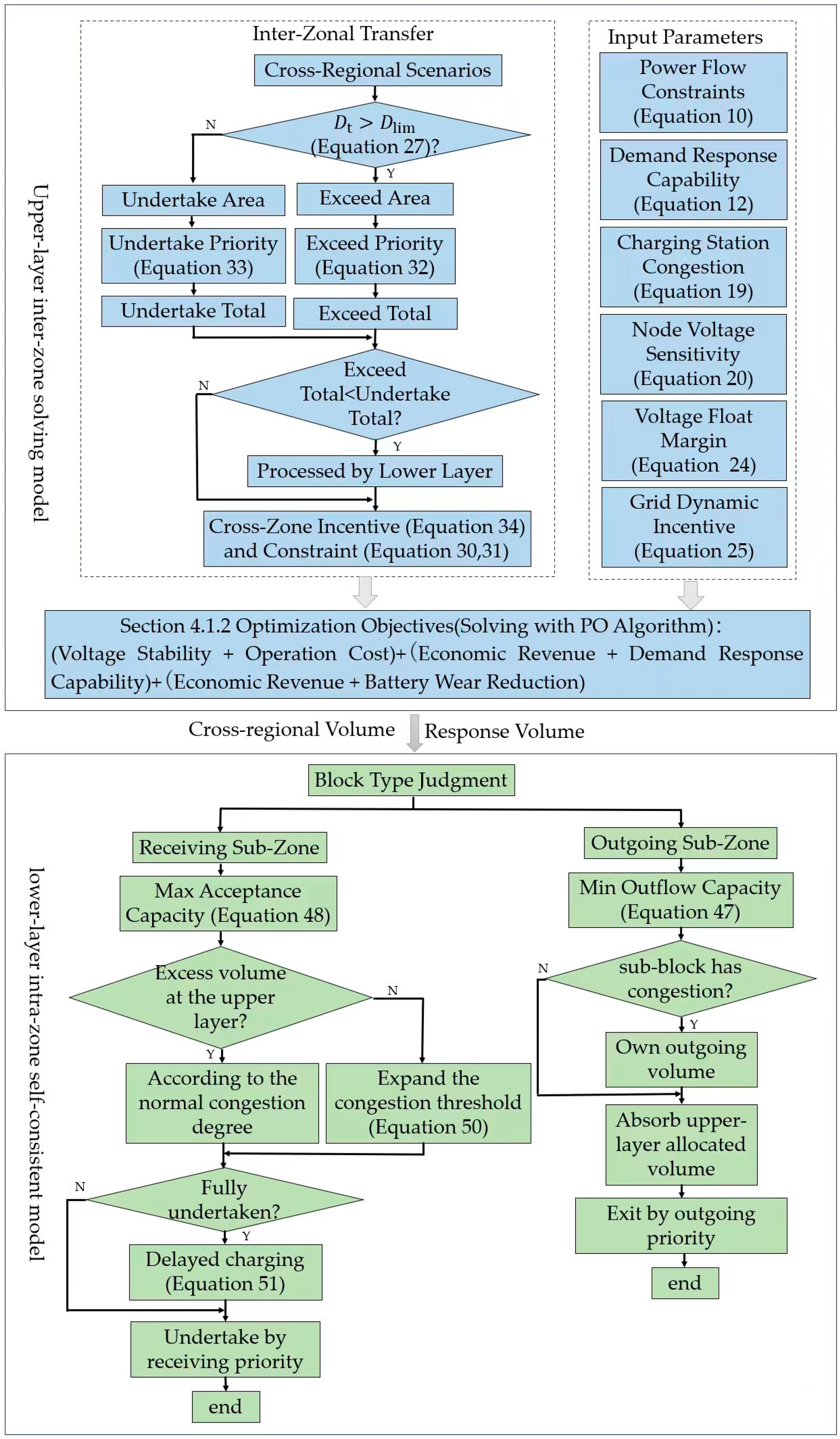
Overall, the specific flow chart is shown in Figure 2.

The core mechanism is elaborated in detail as follows:

• The electric vehicle load in each functional region is predicted using the travel-chain-based Monte Carlo method, and the photovoltaic power output is forecast using the RIME-CNN model.
• Establish an evaluation model for the demand response potential of users. Based on the Fogg Behavior Model, the required SOC and remaining parking duration are obtained from the EV load prediction module mentioned earlier.
• Construct a floating-threshold band with a voltage margin to mitigate the impacts of various intra-day uncertainties.
• Develop a dynamic incentive mechanism between the distribution network and charging stations to encourage active participation in demand response.
• Establish a bi-level collaborative-scheduling model consisting of inter-zone coordination and intra-zone self-consistency.

The upper level implements an inter-zone power exchange mechanism. According to the different requirements of the grid and charging stations, various inter-zone operation scenarios are defined to achieve mutual-support scheduling. The inter-zone mechanism and the demand response potential of charging stations derived from the Fogg Model are incorporated into the objective function. Meanwhile, voltage quality; economic benefits of the grid, charging stations, and users; and the dynamic grid–station incentives are comprehensively considered. Corresponding constraints are constructed for the optimization variables, and the voltage floating-threshold band is embedded into the grid voltage constraints. The PO optimization algorithm is adopted for the solution.

The lower-level model allocates and accommodates the inter-zone power exchange results obtained from the upper level within each zone by introducing a relaxed congestion threshold and a delayed-charging mechanism. A cross-sub-zone mechanism is also introduced within the zone to prevent congestion at charging stations in sub-zones, thereby achieving accurate matching between scheduling objectives and practical operating conditions.

5. Case Analysis

5.1. Simulation System and Data Settings

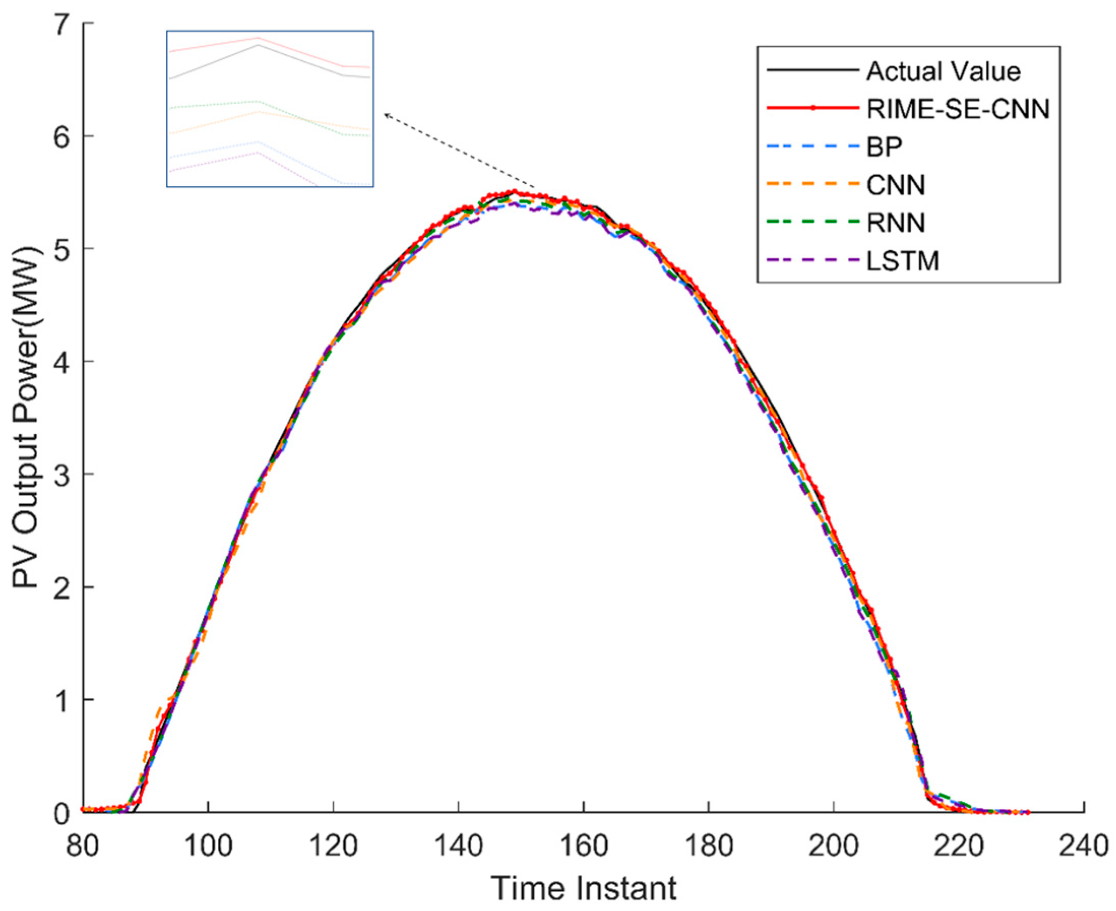
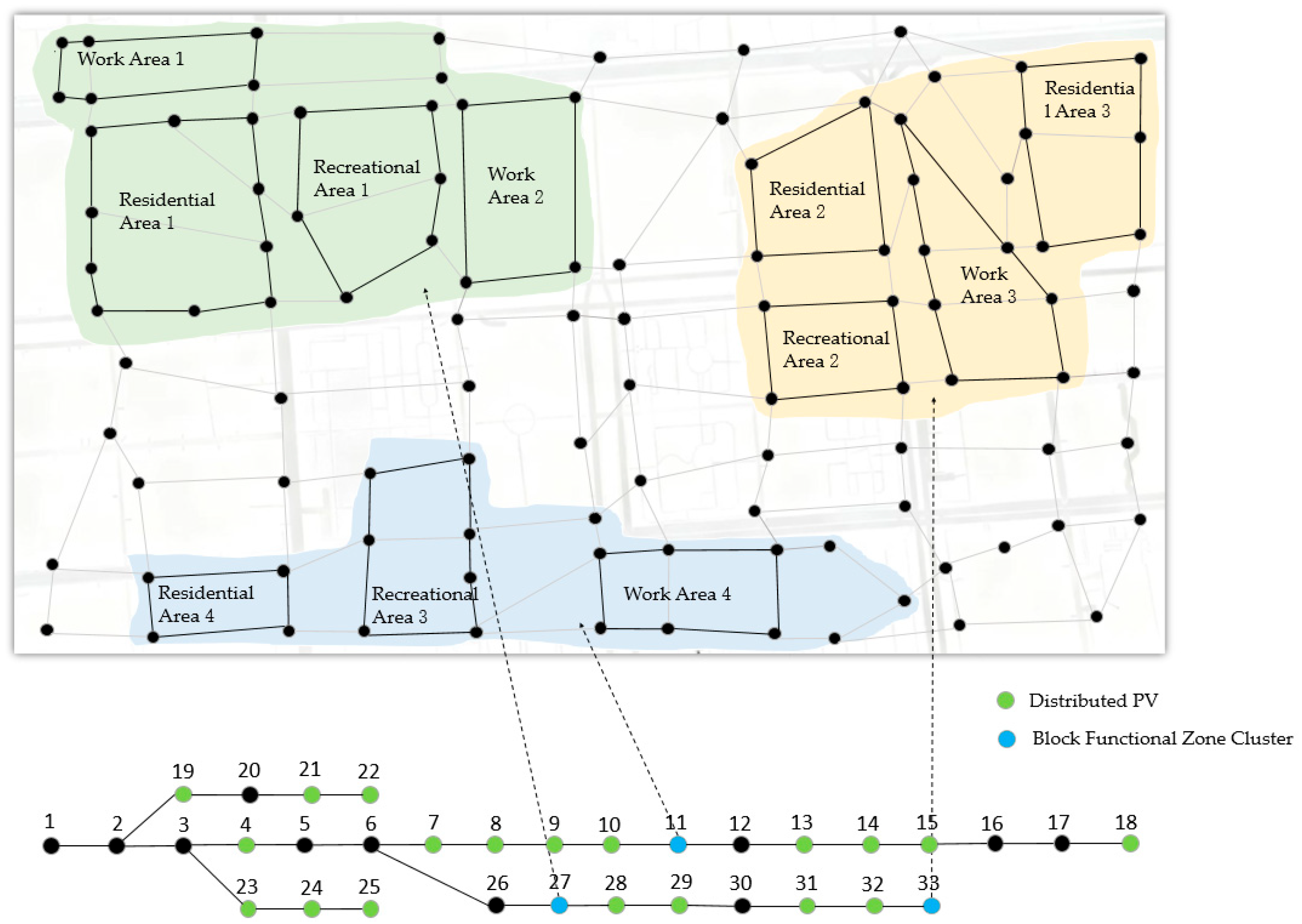
All simulation experiments in this study were completed based on the MATLAB R2021b software environment, and the hardware platform for simulation operation was a computer equipped with an Intel Core i9-12700H processor, which can meet the computing requirements of the scheduling model proposed in this paper. In this paper, the IEEE 33-bus system is adopted as the simulation case, with a rated voltage of 110 kV. The standard conductor type LGJ-300/40, which matches the 110 kV voltage level, is uniformly used in the simulation. The system load comprehensively covers various types including residential, commercial, school, hospital and industrial loads, and its composition is consistent with that of an actual regional distribution network, with a total load set to 48 MW. PV units are connected in a distributed manner, with a total installed capacity of 59 MW. PV output forecasting is carried out using a convolutional neural network algorithm improved by the RIME optimizer, and the detailed forecasting results are displayed in Figure 3. The sampling interval is set to 5 min, resulting in a total of 288 time instants throughout a day. Three zones are configured in the simulation, each mapped to an abstract power grid node of the IEEE 33-bus system, and each zone is further divided into multiple functional areas of different types, as illustrated in Figure 4.

This paper selects small and medium-sized pure electric vehicles as the research object, and the total number of electric vehicles is set to 25,000 [38]. Specifically, the number of charging piles is 100 in residential zones, 80 in working zones, and 40 in leisure zones. The rated charging power of each charging pile is 30 kW, the rated capacity of EV batteries is 60 kWh, the travel temperature is set to 28 °C, and the travel speed is 50 km/h. Other parameters are shown in Appendix A. The basic time-of-use electricity price is presented in

Table 1. Time-of-use electricity price.

Time Period	Time Period Type	Time-of-Use Electricity Price/(¥/kWh)
23:00–00:00	Valley Period	0.43
00:00–7:00	Valley Period	0.43
7:00–17:00	Flat Period	0.58
17:00–20:00	Peak Period	0.68
22:00–23:00	Peak Period	0.68
20:00–22:00	Critical Peak Period	0.78

[39].

5.2. EV Load Forecasting Results

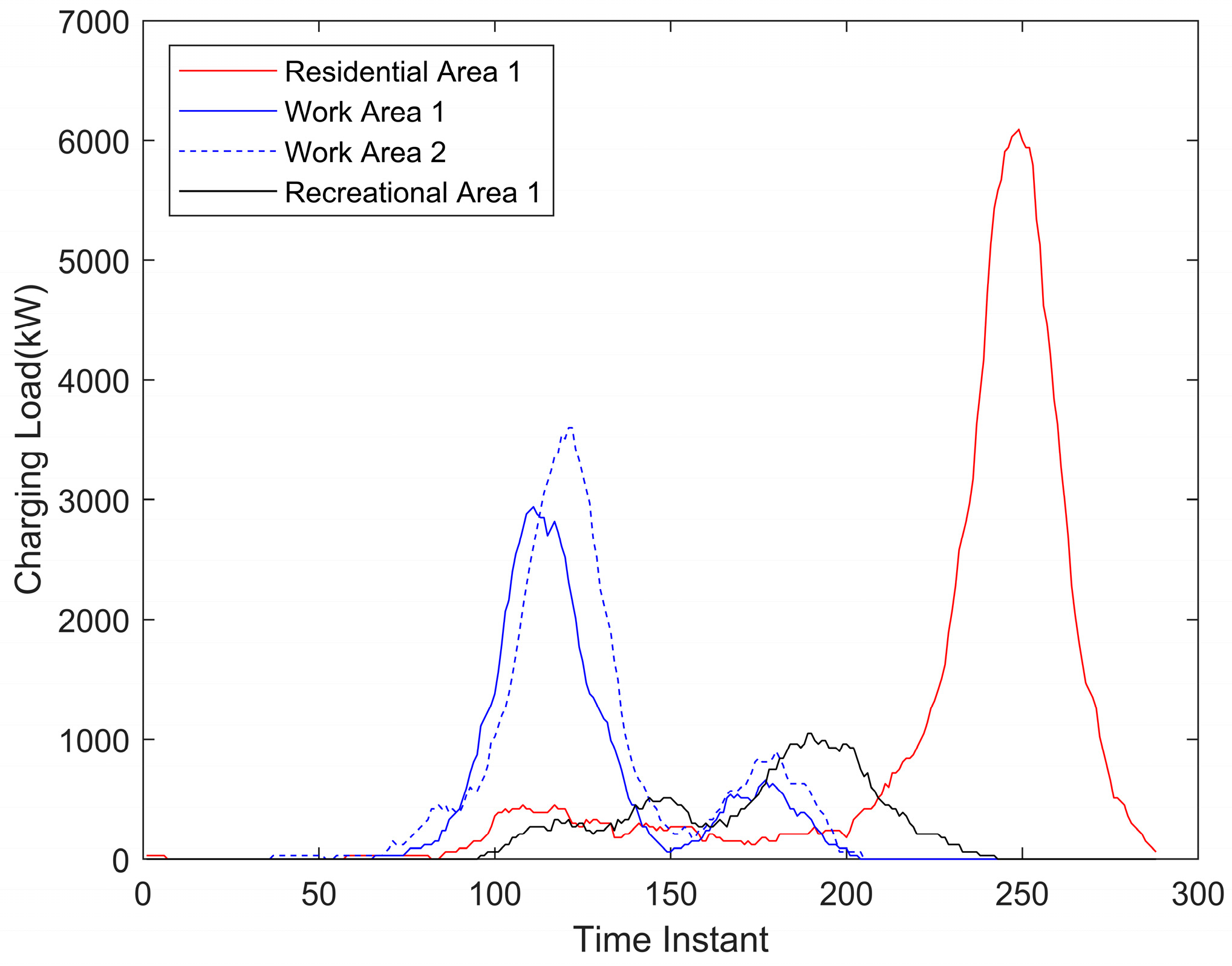
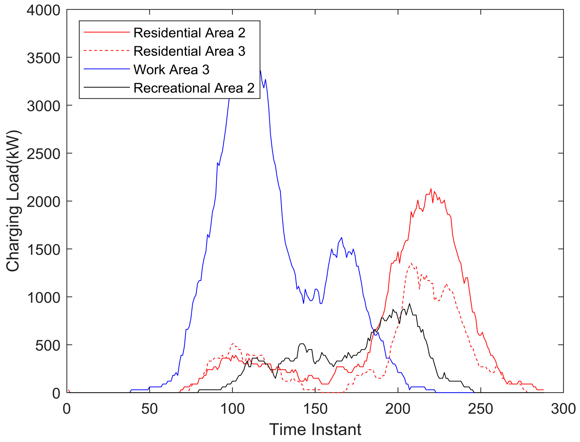
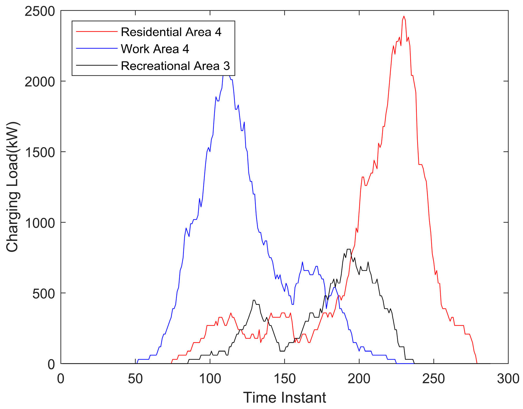
The EV charging load of each zone is shown in Figure 5, Figure 6 and Figure 7. The evening peak of charging load in the residential area concentrates on the period from 18:00 to 22:00, which is caused by users who have completed their daily travel charging centrally after arriving home. Most users in the working area choose to charge after arriving at the workplace between 7:00 and 10:00, while a small number opt for charging at noon. As for the leisure area, users travel both in the morning and afternoon, resulting in two charging peaks.

5.3. Case Comparison Simulation

5.3.1. Case Settings and Algorithm Comparison

Five cases are designed for comparative analysis in the simulation to verify the feasibility of the proposed method by comparing power grid voltage performance, charging station congestion degree, and demand response effectiveness. The detailed settings are as follows:

Case 1: (Blank Control): No demand response is implemented.

Case 2: Neither inter-zone transfer nor the Fogg Model is considered.

Case 3: The Fogg Model is considered, while inter-zone transfer is not.

Case 4: Inter-zone transfer is considered, while the Fogg Model is not.

Case 5: (Proposed Scheme): Both inter-zone transfer and the Fogg Model are considered.

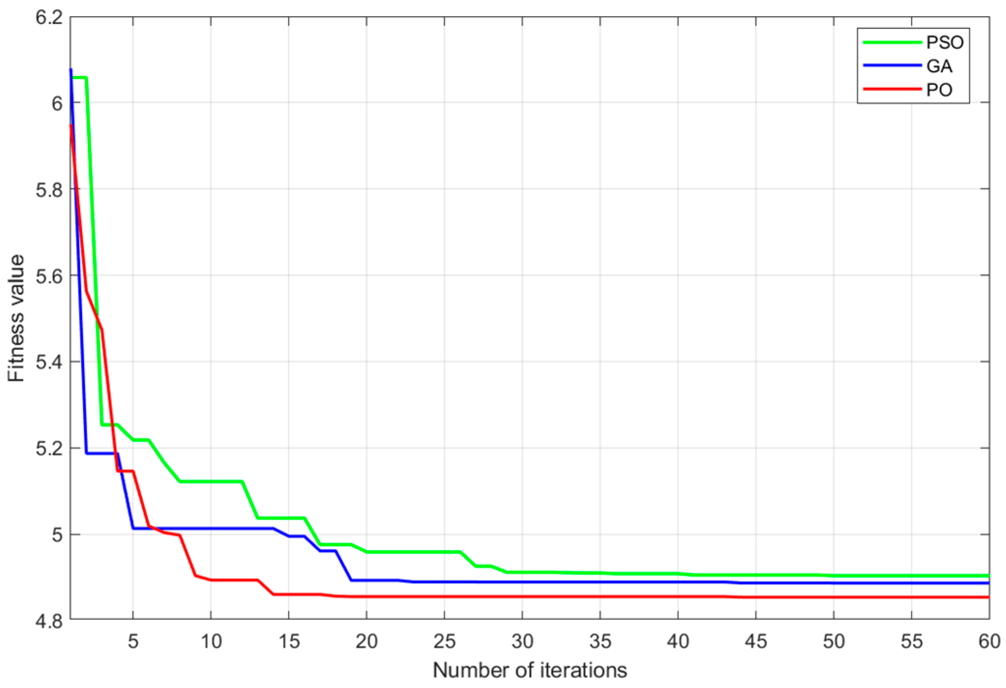
In this paper, the number of iterations is set to 60 and the population size is set to 40. The proposed scheduling method is optimized and solved using the PSO, GA, and PO algorithms, respectively, with the same number of iterations and population size for all algorithms. As can be seen from the comparison in Figure 8, compared with PSO and the GA, the PO algorithm converges faster and achieves better optimization results in the solution process of the model proposed in this paper. It can be seen from

Table 2. Performance comparison of optimization algorithms.

Algorithm Type	Fitness Value	Solution Speed/(s)
PSO	4.90	14,896
GA	4.89	12,338
PO	4.85	10,865

that under this model, the solution efficiency of the PO algorithm is improved by 27.06% compared with the PSO algorithm and by 11.94% compared with the GA. Meanwhile, the optimization accuracy of the PO algorithm is improved by 1.01% compared with the PSO algorithm and by 0.84% compared with the GA.

5.3.2. Result Analysis

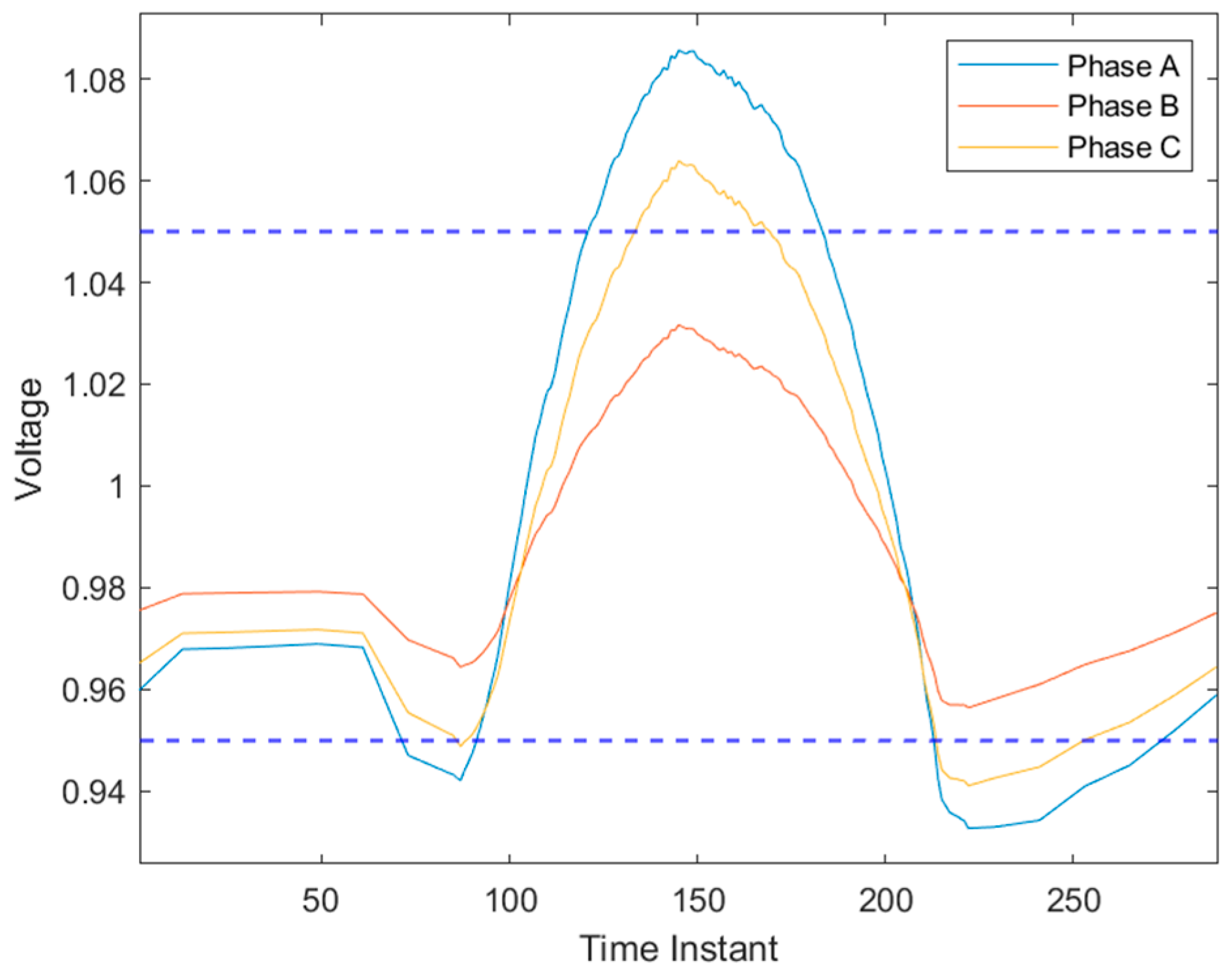
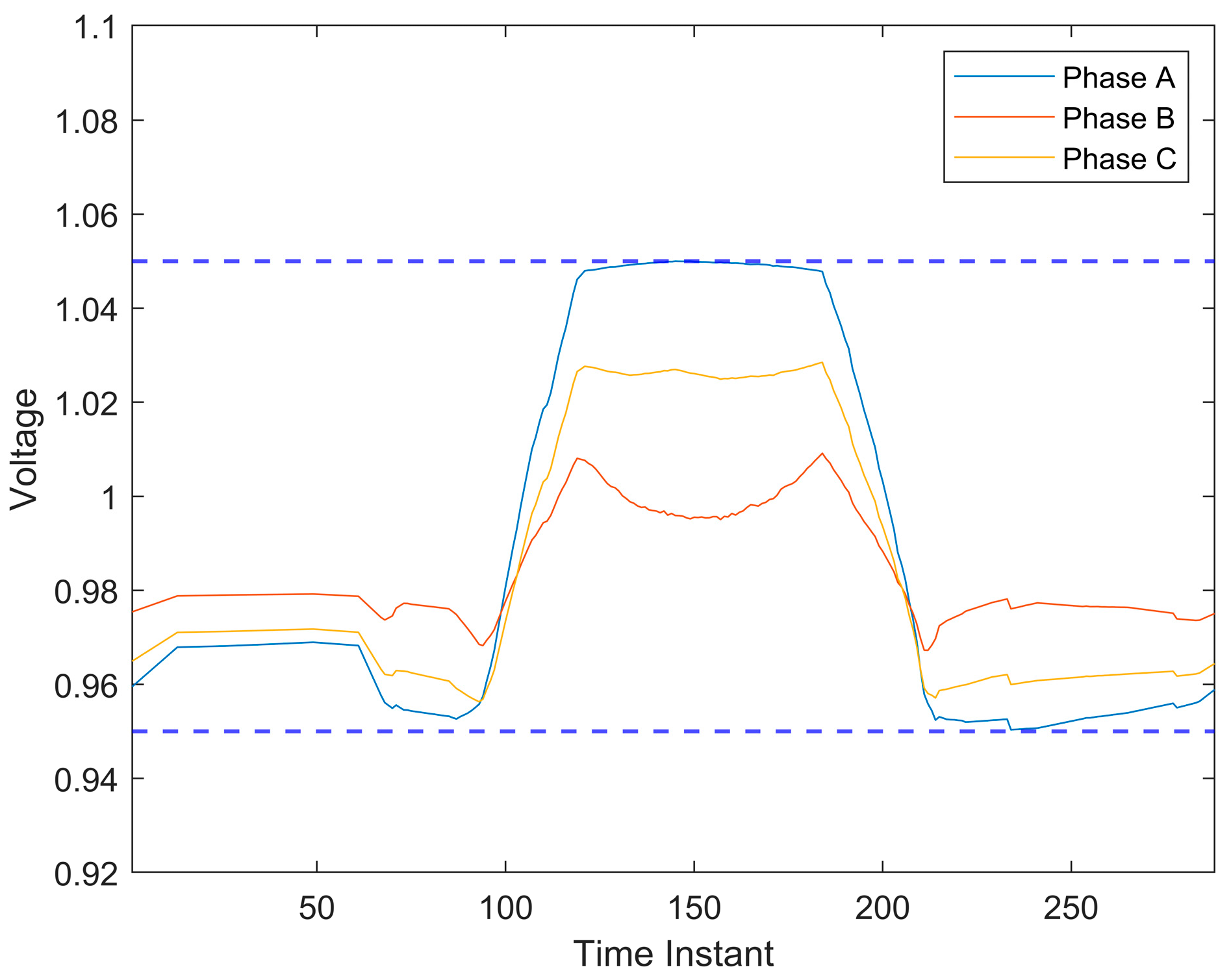
Case 1 (Blank Control): This paper normalizes the voltage data, and according to industry standards, the grid voltage deviation is controlled within the range of ±5%; that is, the normalized voltage value should be in the interval of 0.95~1.05. As is clearly shown in the voltage variation curve in Figure 9, in the operation scenario without any scheduling measures, voltage violations occur during 7:00–8:00 a.m., 10:00–12:00 noon, and 17:00–20:30 p.m., due to the combined effects of PV output randomness, EV charging randomness, and various electrical loads.

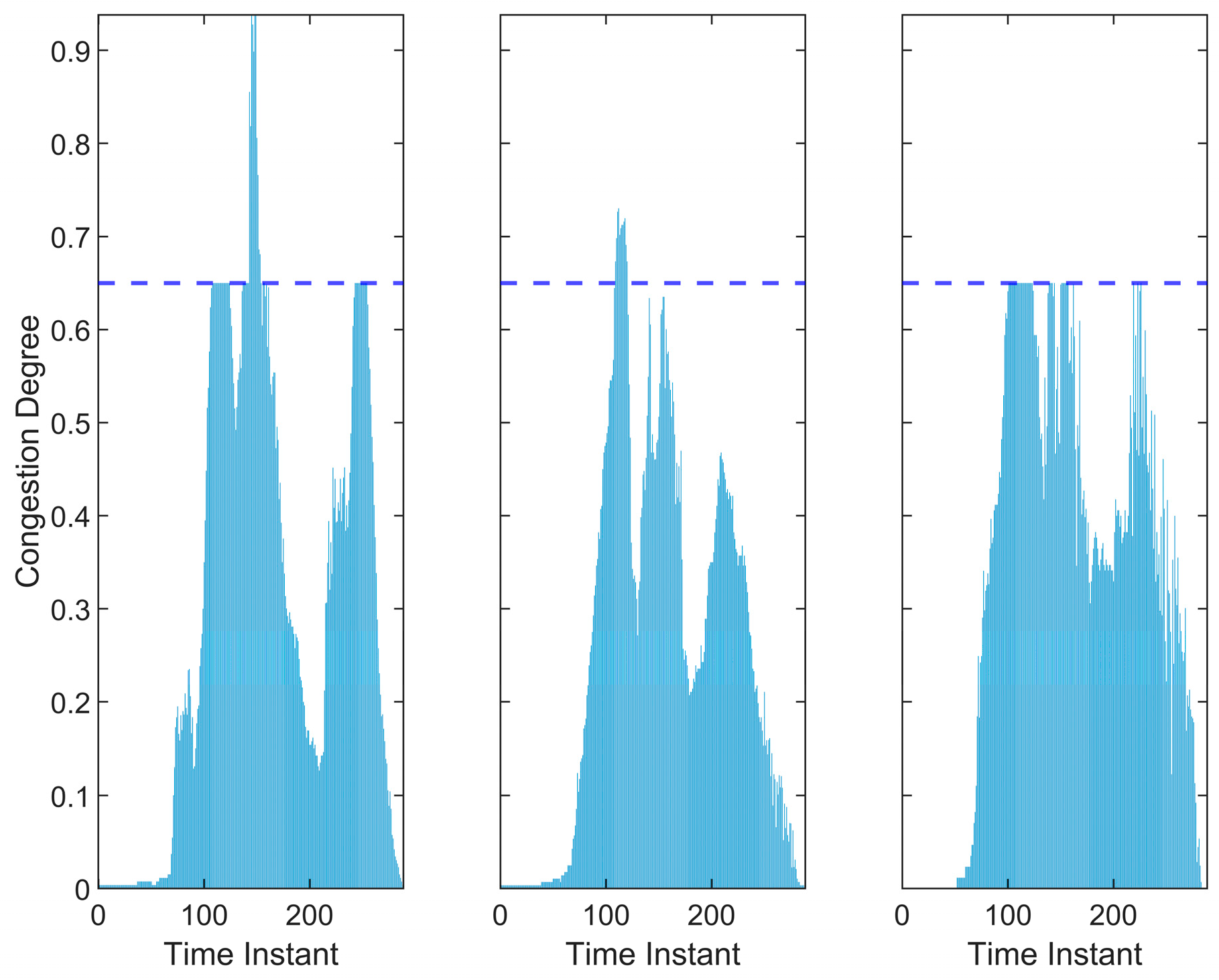
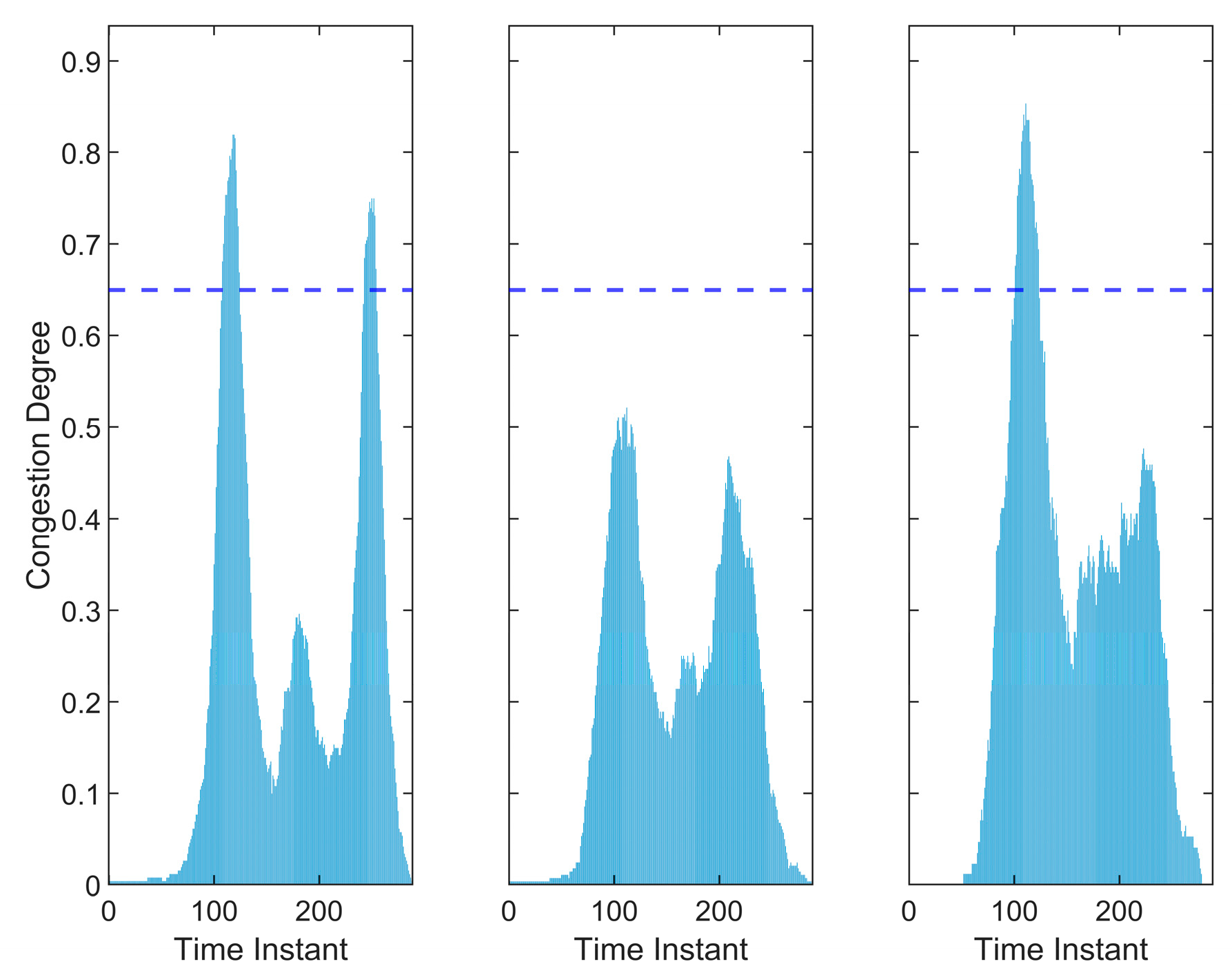
Figure 10 presents the variation in EV charging congestion degree in different zones under the random-user-charging mode. The peak–valley variation trend of congestion degree is consistent with that analyzed in Section 5.2. The unordered charging congestion degrees of different functional areas within the zone are presented in Case 5.

Case 2: Compared with Case 1, the voltage level is significantly improved in Figure 11 through the bidirectional charging and discharging of EV. However, limited by the lack of inter-zone coordinated scheduling, the problem of voltage exceeding the upper limit remains unresolved during 12:00–12:45 noon. The average voltage deviation is adopted as the evaluation index of power grid voltage quality. To make the voltage optimization effect more prominent, this paper selects the typical time period T_y when the voltage of the original power grid exceeds the limit for data collection, specifically 7:00—8:00 a.m., 10:00—12:00 noon, and 17:00—20:30 p.m. The collected data are subjected to normalization processing, as shown in Equation (60). It can be observed from Table 2 that the voltage quality of Case 2 is improved by about 46% compared with Case 1.

$$\delta v_T={\displaystyle \frac{{\displaystyle \sum _{t=1}^{T_{\mathrm{y}}}{v}_t-}{v}_e}{{\mathrm{T}}_{\mathrm{y}}\Delta v_{\max }}}$$

(60)

where $\delta v_T$ is the average voltage deviation of the power grid during the original voltage over-limit time period ${\mathrm{T}}_{\mathrm{y}}$; $v_e$ is the rated power grid voltage; and $\Delta v_{\max }$ is the maximum voltage deviation.

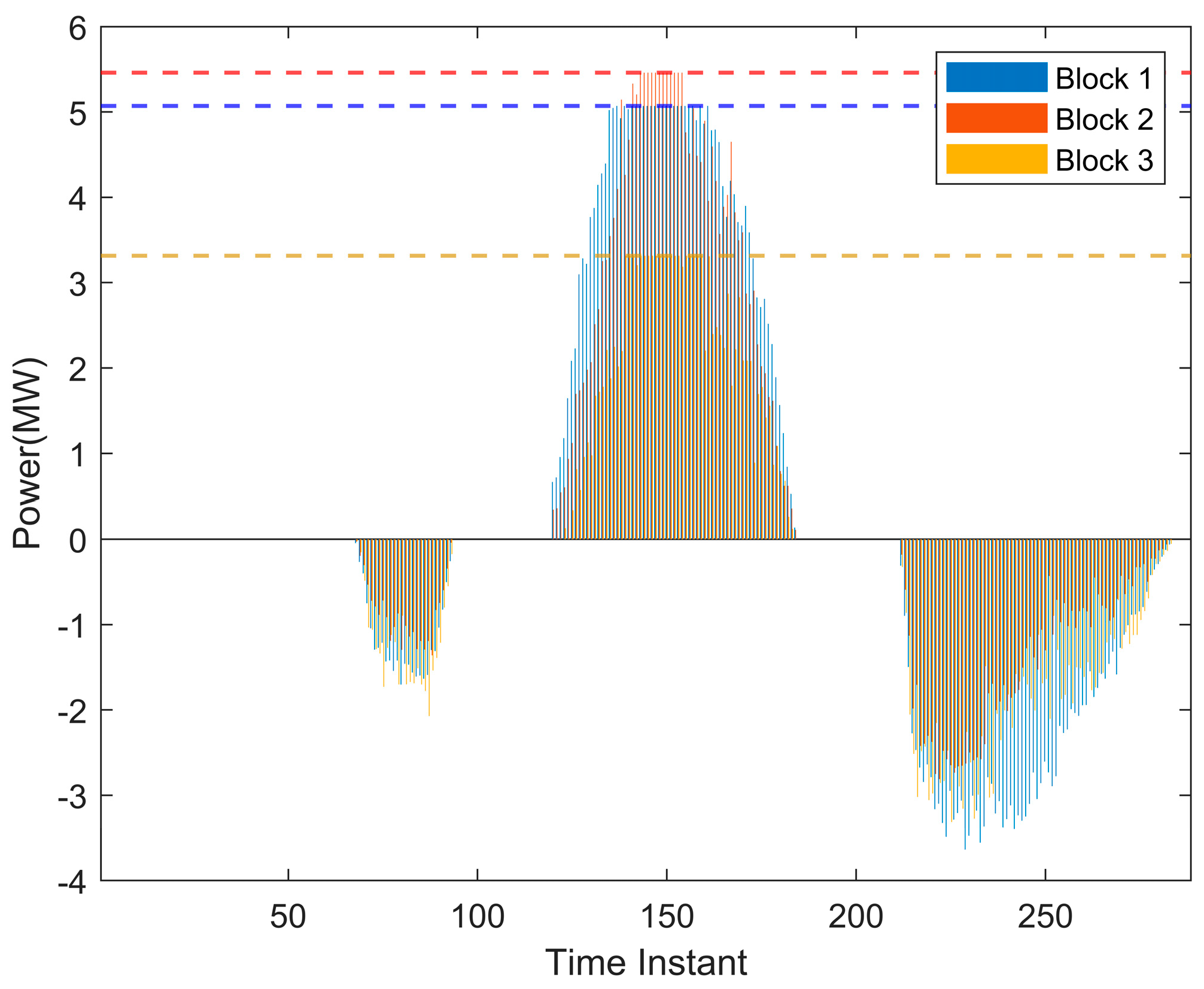
As can be seen from Figure 12, Case 2 does not consider the demand response capacity of each zone, leading to zones with high voltage regulation sensitivity prioritizing power output. However, this approach ignores the inherent response capacity of each zone, resulting in unbalanced demand response.

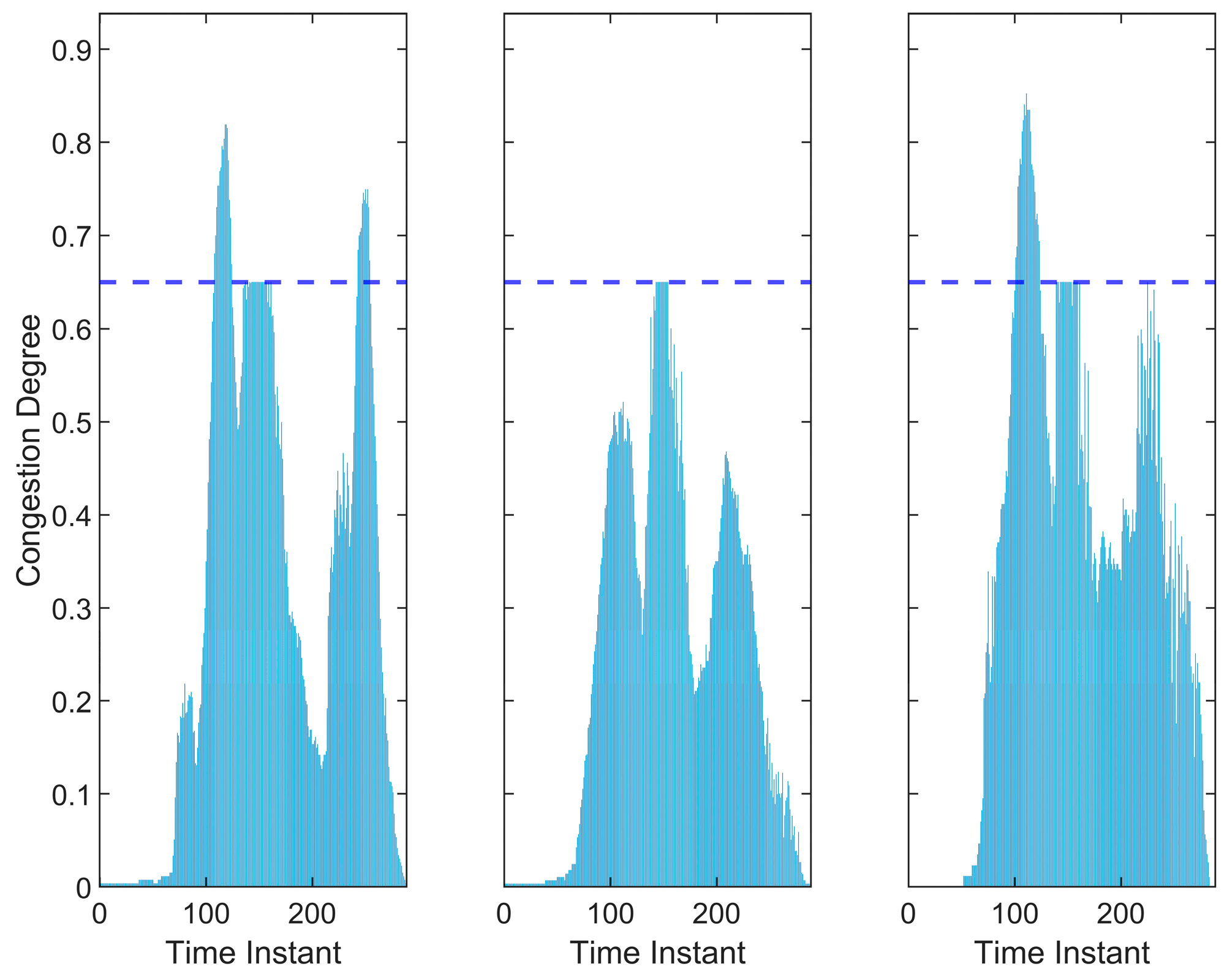
It can be observed from Figure 13 that the charging congestion problem of zone charging stations remains unresolved. Zone 1 participates in demand response the most, and its congestion degree increases significantly during 7:00–8:00 a.m., 10:00–12:00 noon, and 17:00–20:30 p.m.—consistent with the voltage violation time periods in Case 1.

Case 3: As shown in Figure 14, the voltage over-limit problem during 12:00–12:45 noon remains unresolved, consistent with Case 2. In the tripartite optimization, Case 3 prioritizes the participation degree of demand response. It can be seen from Table 2 that the voltage quality of Case 3 increases by approximately 11% compared with Case 2.

This case takes into account the demand response capacity of each zone. As indicated in Figure 15, the balance degree between the three zones is defined by Equation (41). Calculations show that compared with Case 2, the balance degree is improved by 52.31% during 7:00–8:00 a.m. and 17:00–20:30 p.m.

From the results in Figure 16, benefiting from the consideration of demand response capacity, the congestion degree of Zone 1 during 12:00–12:45 noon is significantly reduced. However, similar to Case 2, the lack of inter-zone transfer results in the failure to fundamentally solve the congestion problem.

Case 4: As can be seen from Figure 17, the voltage over-limit problem has been solved by guiding the cross-zone scheduling of electric vehicles, and the voltage quality is improved by approximately 36% compared with Case 3.

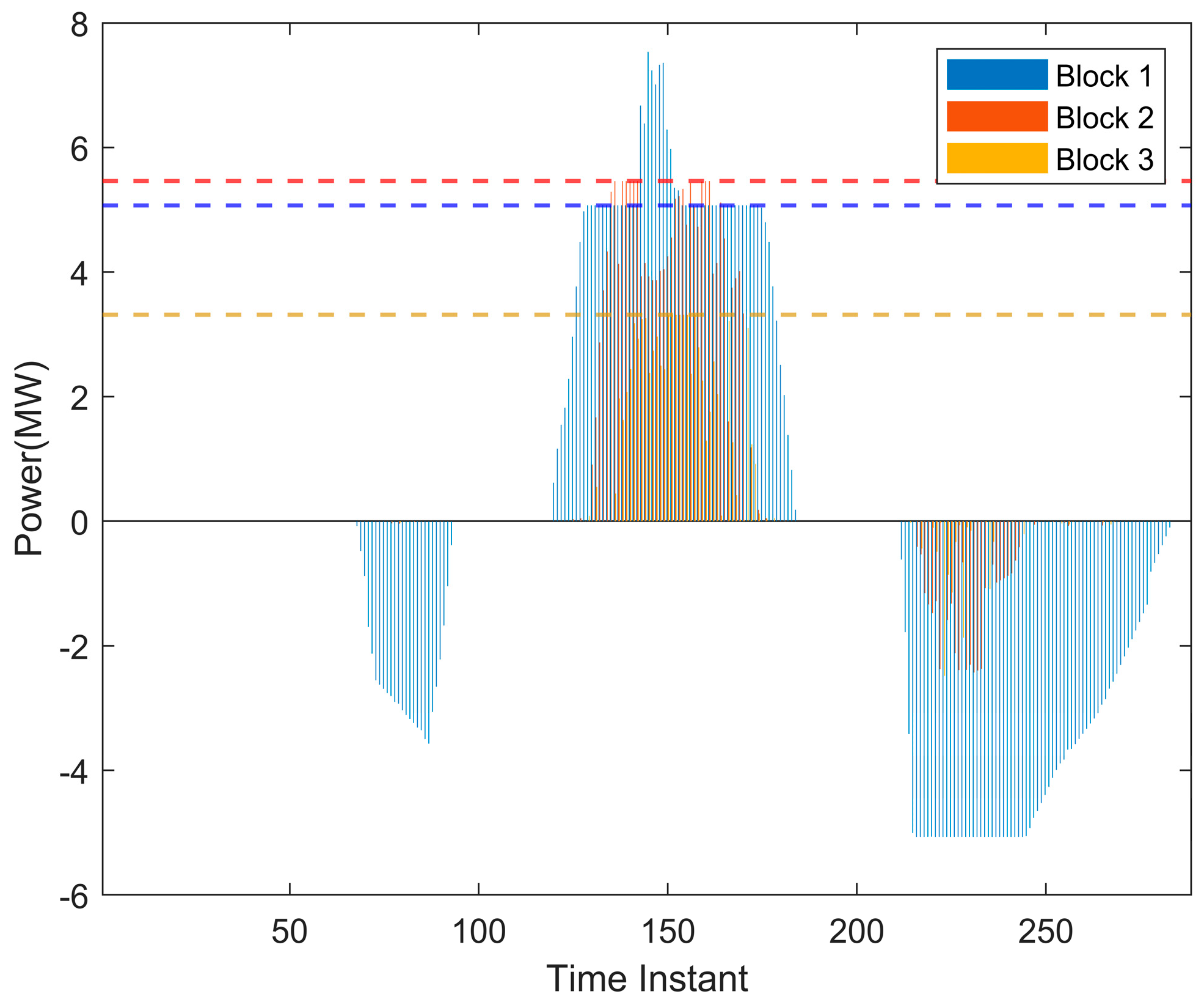
However, as this is a control case without considering the demand response capability of charging stations, the response results do not match the actual response potential, which further leads to an imbalance in demand response across the three zones, as shown in Figure 18.

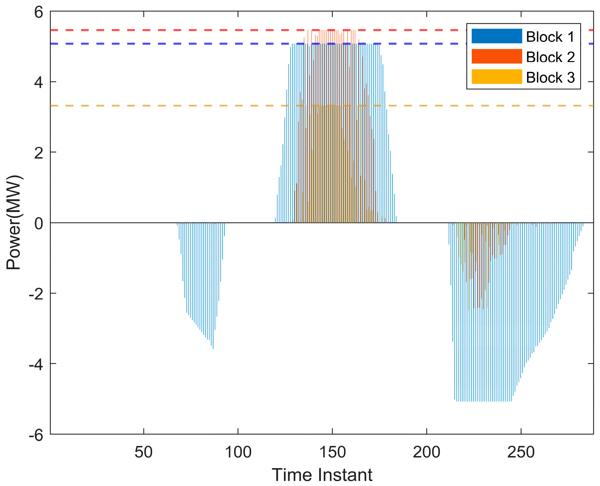
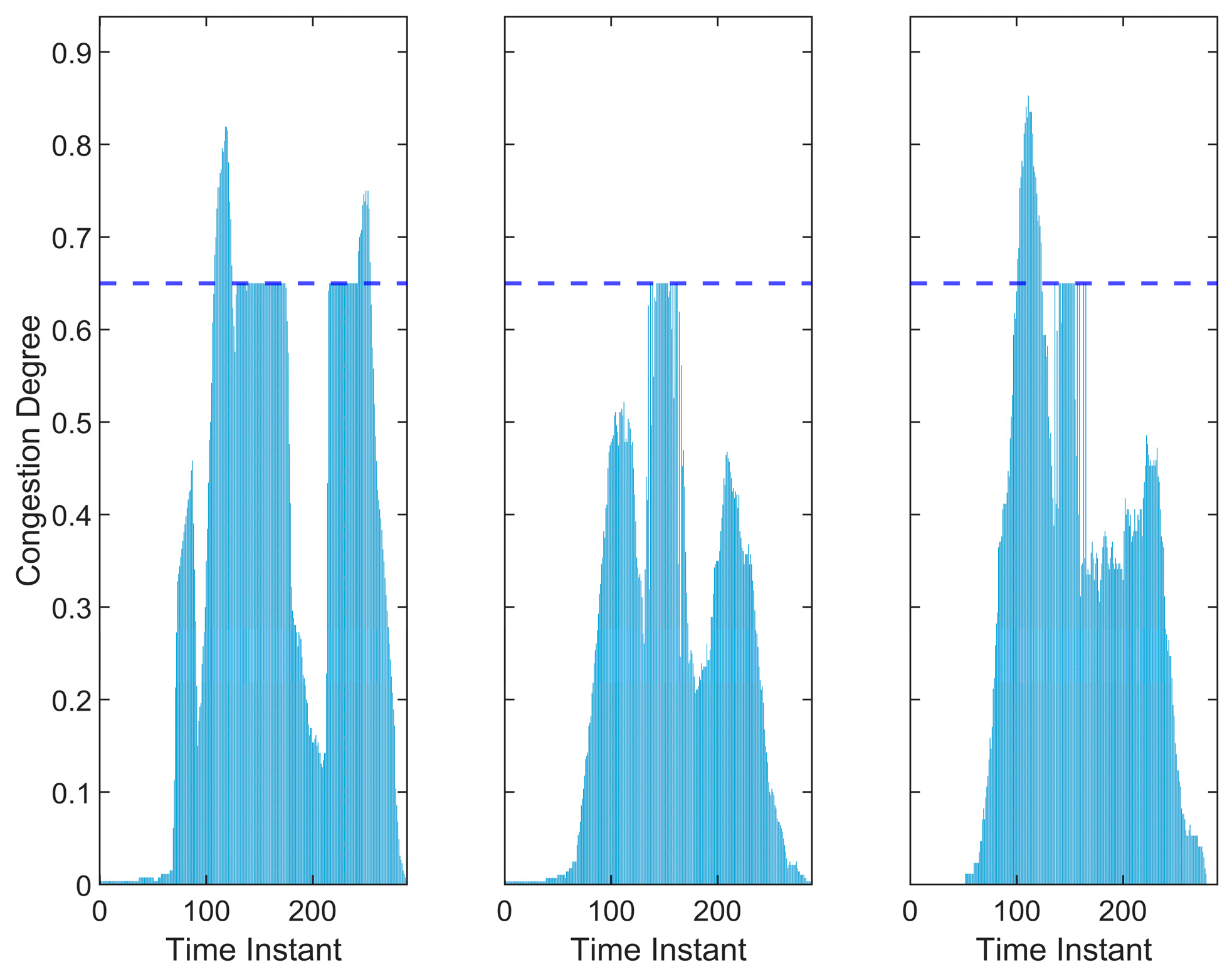
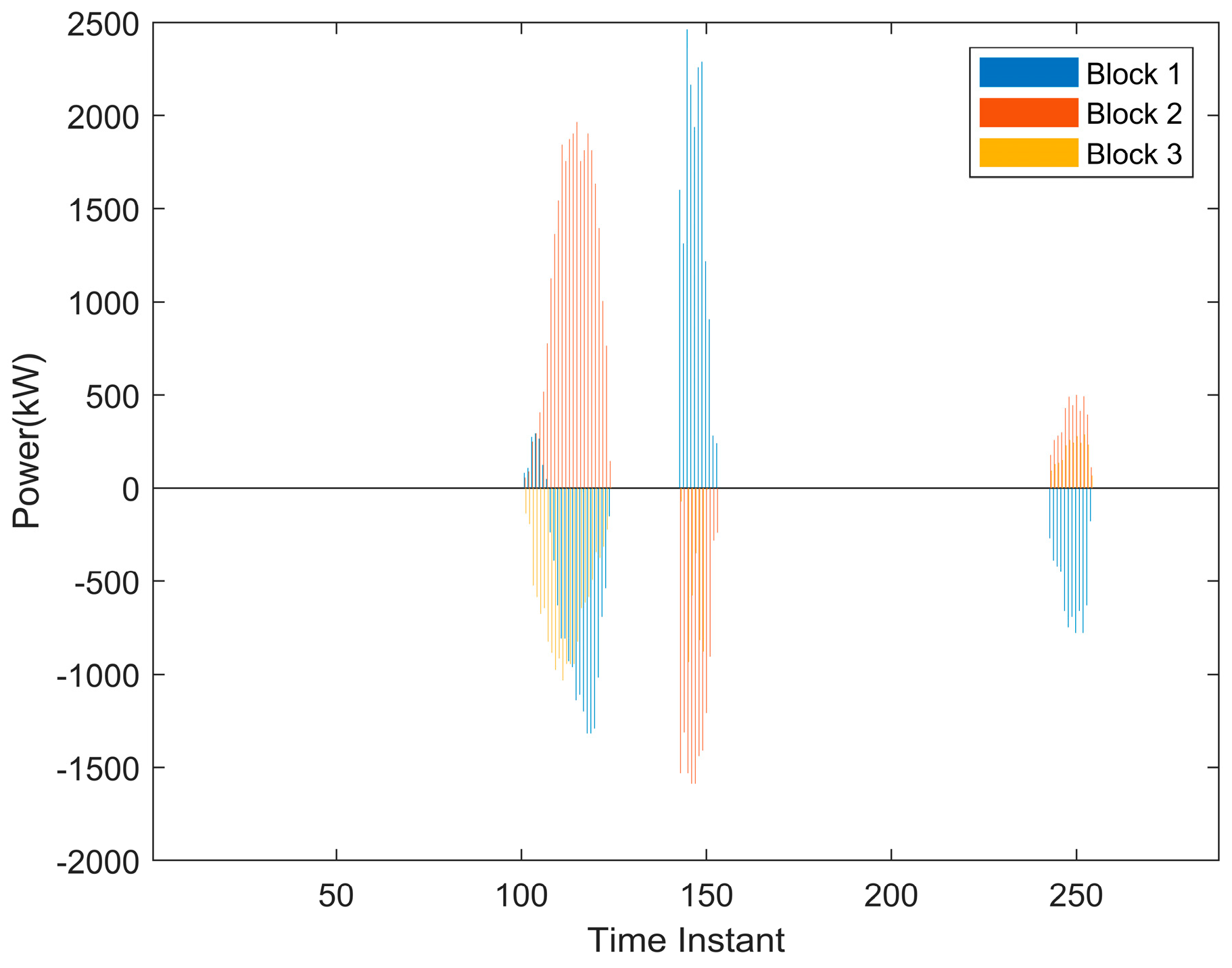
It can be concluded from Figure 19 and Figure 20 that cross-zone transfer is triggered by voltage over-limit during 12:00–12:45 noon. EVs are scheduled to charge from Zones 2 and 3 to Zone 1, resulting in the congestion degree of Zone 1 exceeding the threshold during this period.

During 8:30–10:30 a.m. and 20:20–21:00 p.m., cross-zone transfer is triggered by excessively high congestion degree. Zone 2 serves as the main receiving zone, leading to severe congestion in Zone 2 during 10:00–10:30 a.m. At this point, inter-zone transfer alone can no longer meet the congestion relief demand, requiring further processing at the lower layer.

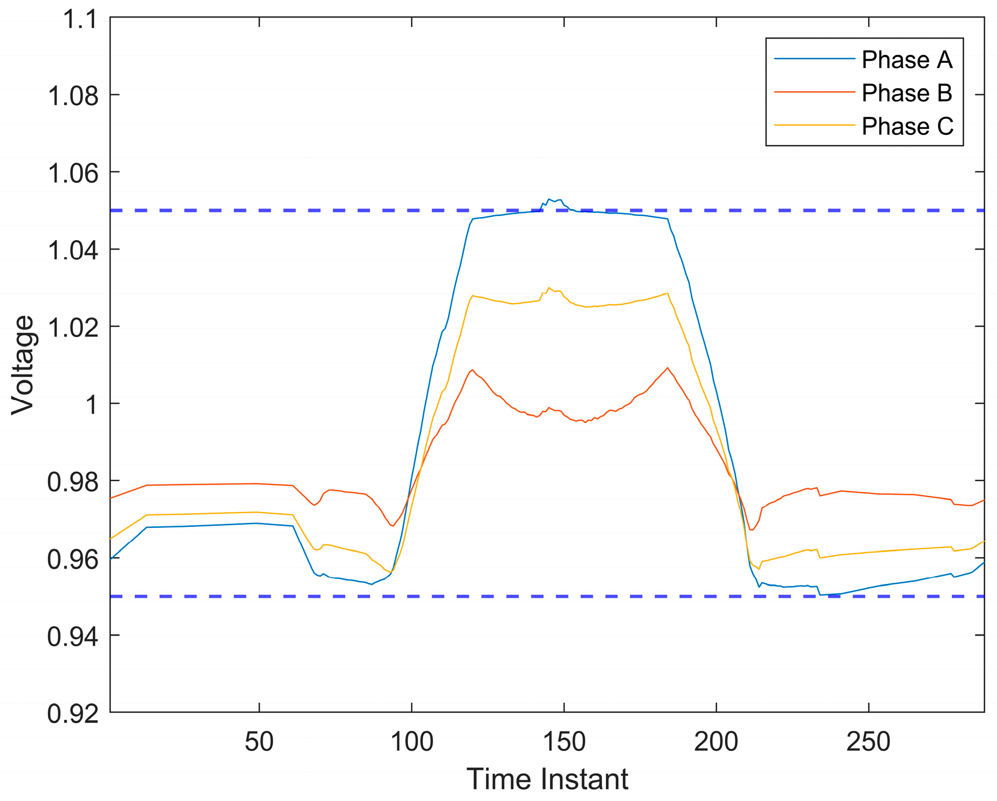
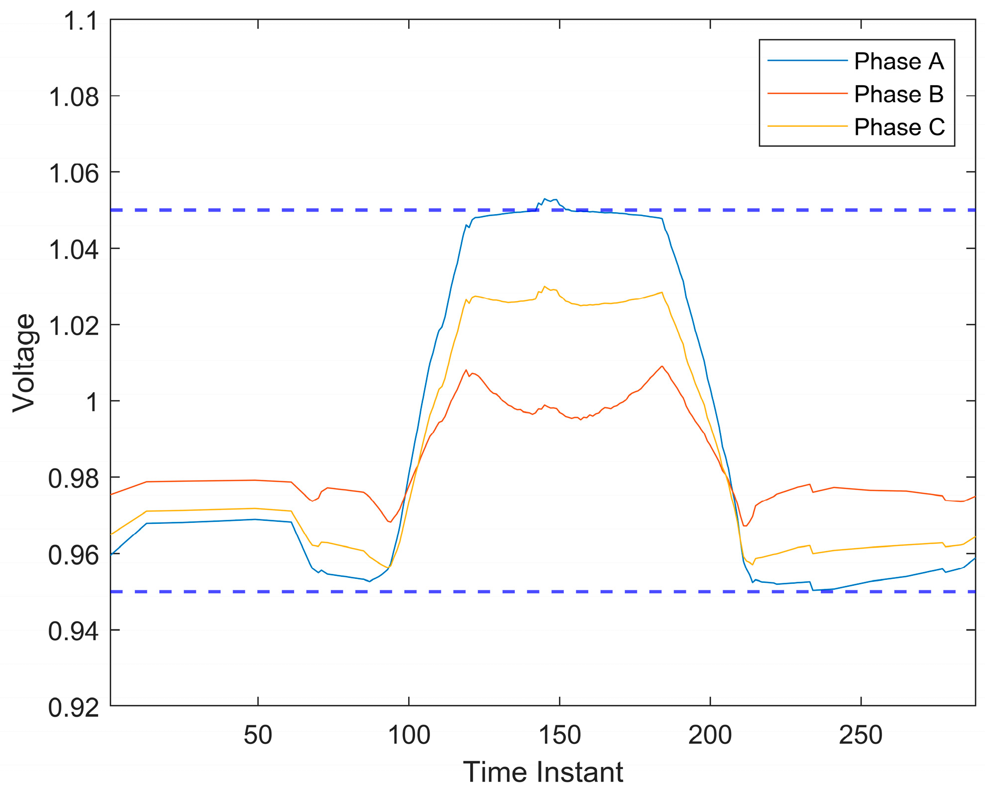
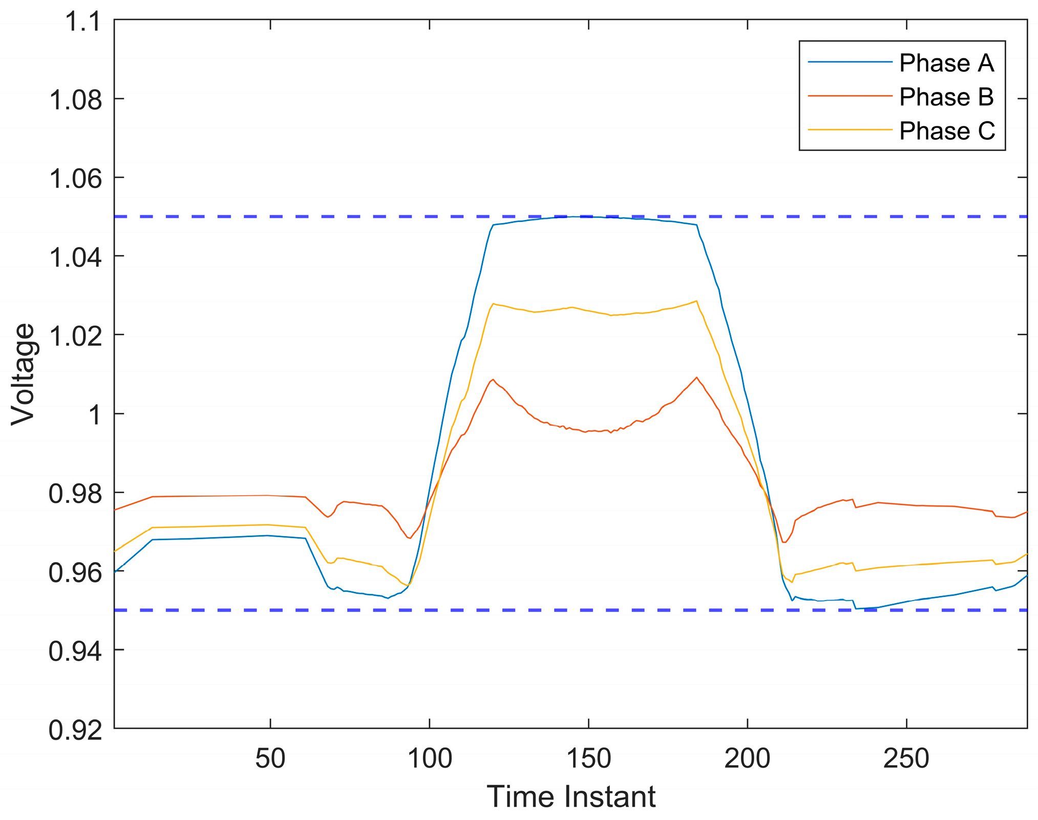
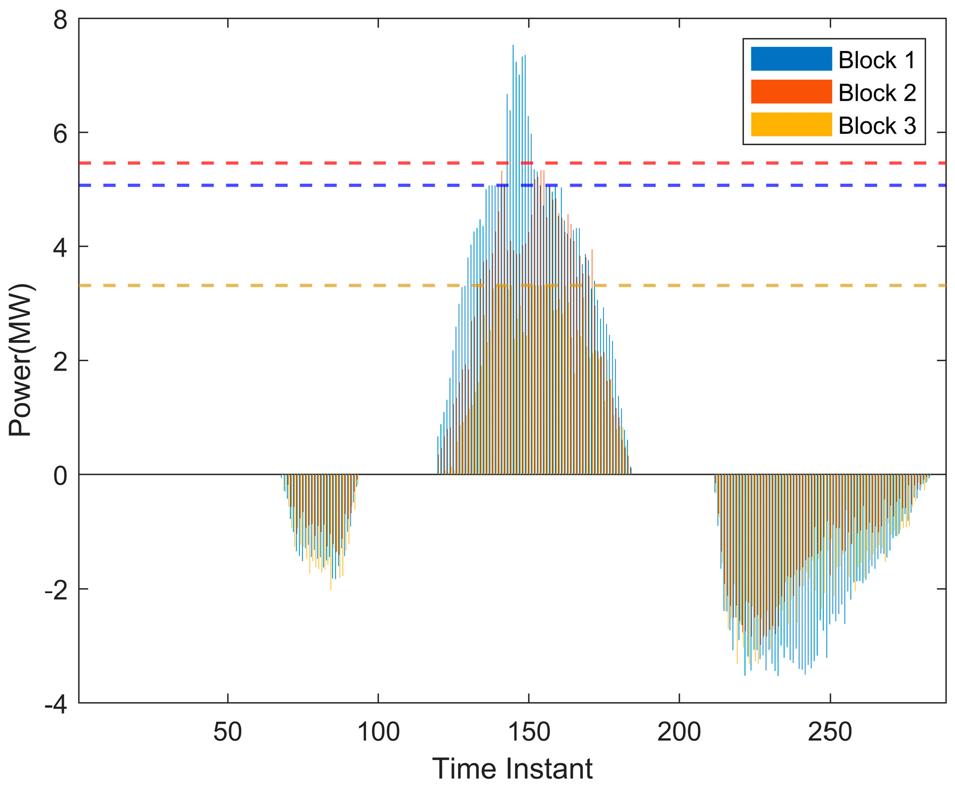
Case 5 (Proposed Scheme): As shown in Figure 21 and Figure 22, consistent with Case 4, the inter-zone transfer mechanism is introduced in this case, thereby completely solving the voltage over-limit problem. Compared with Case 4, the response volume of Zone 1 is generally reduced, while that of Zones 2 and 3 is increased, realizing balanced power output among the three zones. Calculations indicate that the balance degree is improved by 43.58%. Compared with Case 4, Case 5 introduces the demand response potential of charging stations evaluated based on the Fogg Behavior Model, which effectively improves the balance degree of demand response in charging stations, ensures the accurate matching between user demand response potential and the demand response volume issued by charging stations, and realizes the coordinated optimization of voltage regulation and demand response balance.

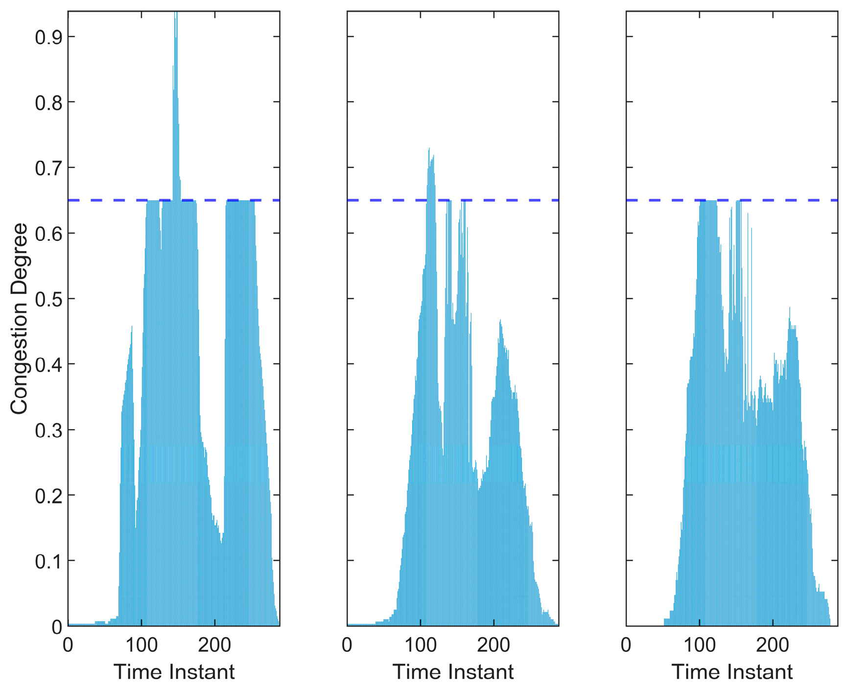
It can be observed from Figure 23 that compared with Case 4, the congestion degree of Zone 1 (with high voltage regulation sensitivity) is significantly improved. The congestion problems during 7:00–8:00, 10:00 a.m.–12:00 p.m. and 17:00–20:30 p.m. have been completely solved. During 8:30–10:30 a.m. and 12:00–12:45 noon, the congestion degree in Zone 1 and Zone 2 exceeds the threshold, yet it still remains below the actual upper limit that the charging stations can withstand. This phenomenon is mainly caused by inter-zone scheduling. Given that the safe operation of the power grid is taken as a hard constraint in this paper, the method of expanding the congestion threshold is adopted accordingly.

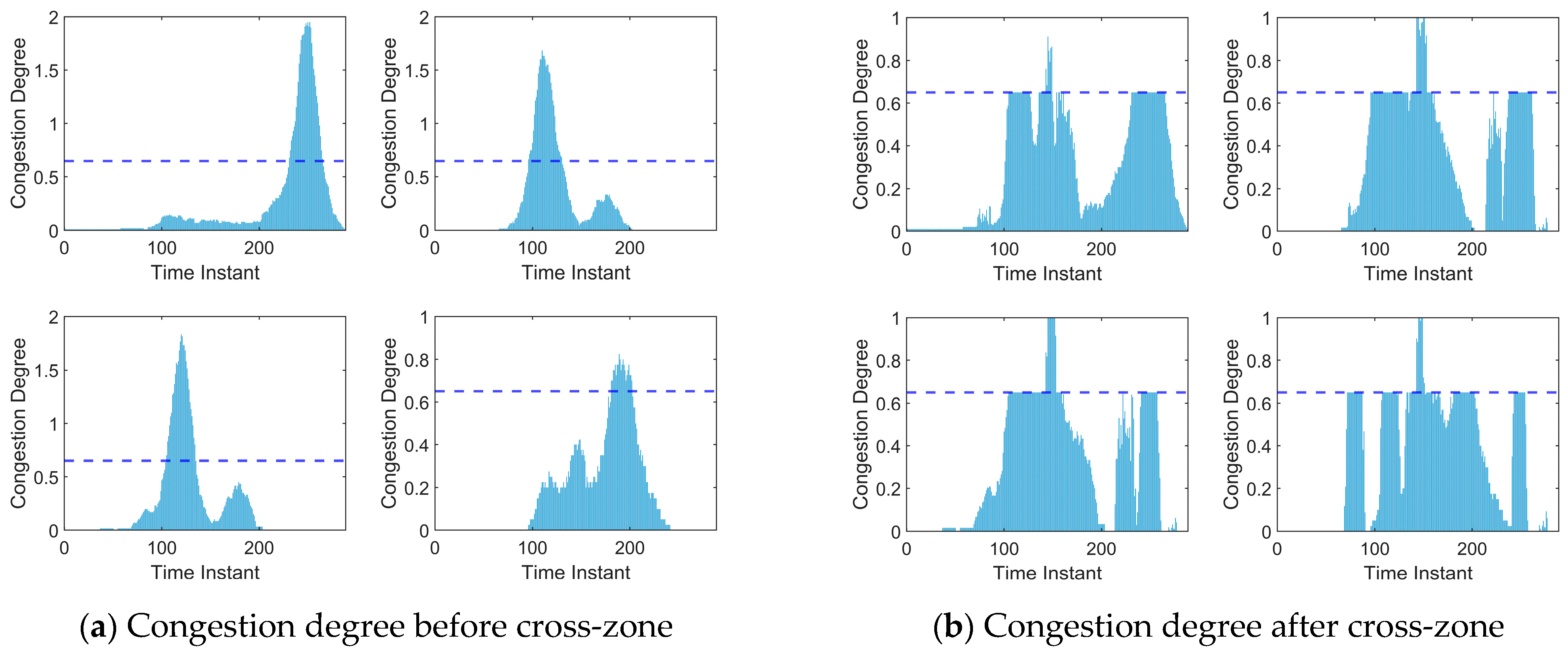
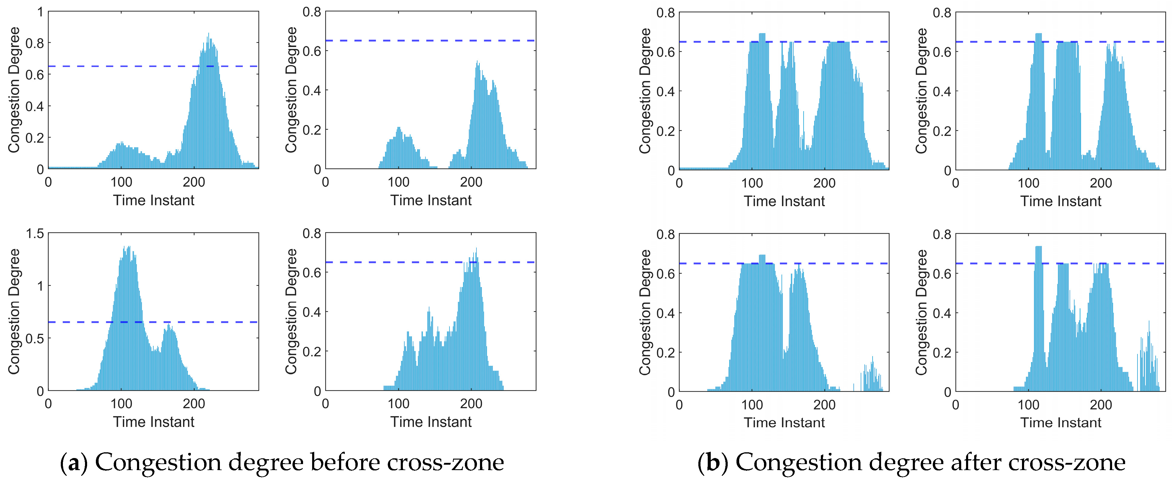
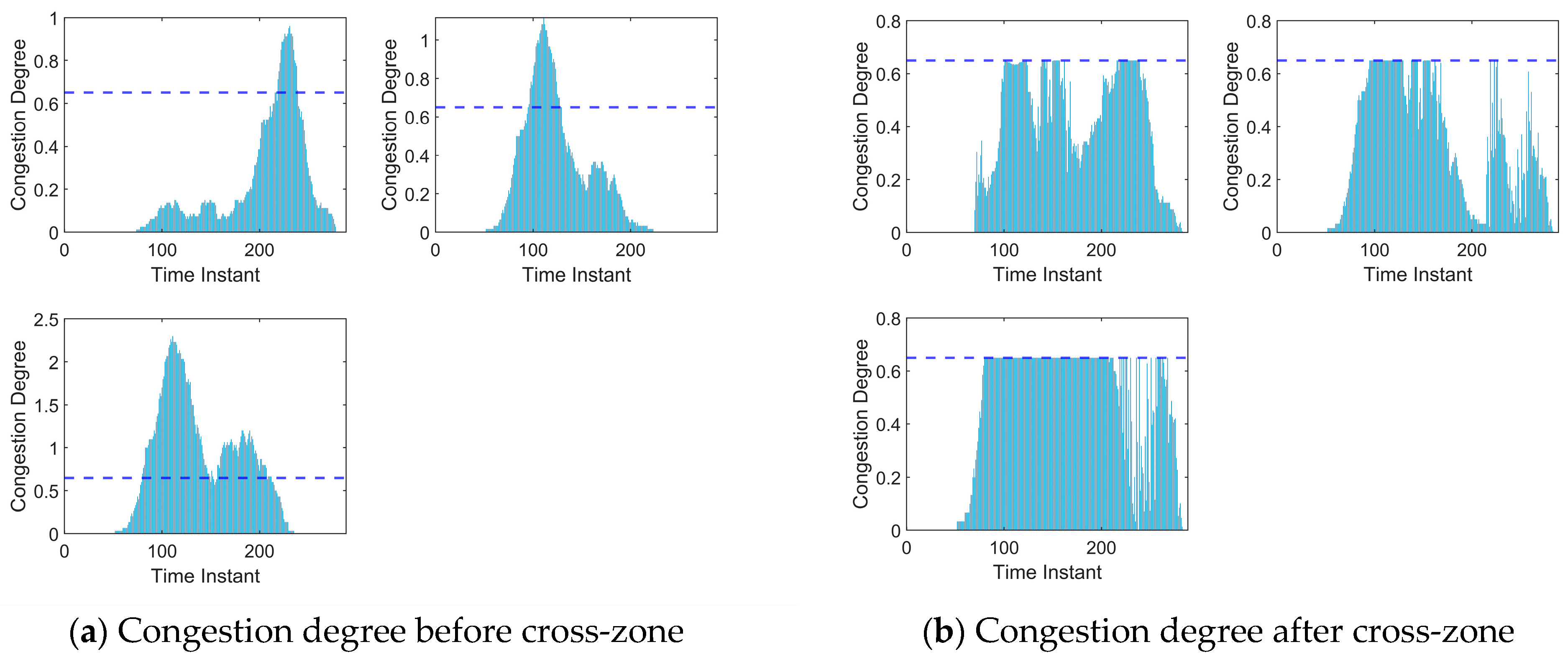
In Figure 24, Figure 25 and Figure 26, Subfigure (a) shows the sub-zone congestion degree before cross-regional transmission, and Subfigure (b) represents that after cross-regional transmission. The lower layer enhances the practicality and flexibility of the proposed scheme by appropriately expanding the congestion degree threshold and adopting delayed charging strategies. Specifically, during 9:00–10:00 a.m. and 12:00–12:45 noon, sub-zones in Zones 1 and 2 expand their congestion degree thresholds to accommodate the transferred charging demand. For Zone 1, after its congestion degree reaches the maximum limit, the excess charging load is diverted to delayed charging.

In summary, regarding power grid voltage improvement, a comparison between Case 1 and Case 2 demonstrates that the introduction of EV demand response effectively enhances the power grid voltage level. In terms of balancing charging station output, comparisons between Case 2 and Case 3, as well as between Case 4 and Case 5, indicate that incorporating the demand response capacity of zone charging stations into the objective function achieves more balanced power output across all zones. For cross-zone regulation, comparisons between Case 2 and Case 4, and between Case 3 and Case 5, show that the introduction of an inter-zone transfer scheduling mechanism not only alleviates the congestion problem of charging stations but also further optimizes the power grid voltage.

As can be seen from

Table 3. Results comparison.

Result Type	Case 1	Case 2	Case 3	Case 4	Case 5
Power Station Revenue (104 ¥/day)	-	56.98	59.81	60.58	64.41
User Revenue (104 ¥/day)	-	58.86	65.09	63.71	69.46
Voltage deviation	0.69	0.37	0.33	0.21	0.23

, since Case 1 serves as a blank control without demand response, it generates no economic benefits during the demand response process. Taking Case 2 as the reference, a comparison with Case 3 reveals that after incorporating the demand response capacity of charging stations, the comprehensive benefits of charging stations and users are proportional to the response volume, increasing by approximately 9%, while the voltage quality increases by about 11% accordingly. Compared with Case 4, the introduction of cross-zone scheduling increases the charging station revenue by approximately 6% due to cross-zone incentive costs, while raising user revenue by 8% and significantly improving voltage quality. As the optimal scheme of this paper, Case 5 demonstrates that considering both the demand response capacity of charging stations and cross-zone scheduling not only markedly enhances the revenues of both charging stations and users, as well as realizing balanced response among all zones, but also completely resolves the voltage over-limit problem.

6. Conclusions

Against the background of large-scale EV integration and high-penetration PV access in power grids, this paper proposes a two-layer cross-zone coordination–autonomy model. The upper layer integrates the Fogg Behavior Model and establishes a cross-zone scheduling mechanism that accounts for charging station congestion. The lower layer absorbs the cross-zone transfer volume and response quantity output by the upper layer, implementing fragmented allocation to achieve the optimal balance among charging station revenue, user revenue, and power grid voltage regulation performance. The PO algorithm is adopted for iterative solution, and comparative case studies verify the effectiveness of the proposed method.

The Fogg Behavior Model introduced in this paper can accurately analyze the uncertain characteristics of user behavior, scientifically quantify the demand response potential of charging stations, effectively improve the feasibility of scheduling schemes, and further promote the balance of demand response among various charging stations. The established two-layer model achieves hierarchical and refined regulation from inter-zone to intra-zone, and exhibits unique advantages in alleviating charging station congestion, optimizing power grid voltage quality, and realizing the global optimization of multi-stakeholder benefits. The results of comparative case analysis show that compared with traditional scheduling strategies, the proposed method can effectively alleviate the problem of charging station congestion, with the balance degree among zones increased by 43.58% and the power grid voltage deviation reduced by approximately 38%.

The proposed two-layer cross-zone coordination–autonomy model possesses practical application value, offering a feasible exploration for solving operational problems of charging stations and power grids. Nevertheless, this study has limitations, and future research will be expanded in the following directions: In terms of model scenario construction, it is planned to expand scenario coverage and supplement boundary scenarios to enhance the model’s adaptability to complex operating conditions. In the algorithm optimization stage, multiple optimization algorithms will be applied to the established model, and comparative analysis will be conducted to provide reliable support for the model’s efficient operation. At the real-time response level, comprehensive quantitative analysis of uncertainties caused by users’ real-time responses will be carried out to improve the model’s robustness.

References

1. Wu, J.; Li, L.; Zhang, J.; Xiao, B. Flexibility Estimation of Electric Vehicles and Its Impact on the Future Power Grid. Int. J. Electr. Power Energy Syst. 2025, 164, 110435. [Google Scholar] [CrossRef]
2. Ardakani, A.H.; Nijenhuis, B.; Hurink, J.; Gibson, I.; Shirazi, E. MDN-MPC: Learning EV Charging Behavior with Mixture Density Networks for Controlling PV Charging Stations. IEEE Trans. Transp. Electrif. 2026. early access. [Google Scholar] [CrossRef]
3. Pavlík, M.; Vojtek, M.; Ševc, K. The Impact of Renewable Generation Variability on Volatility and Negative Electricity Prices: Implications for the Grid Integration of EVs. World Electr. Veh. J. 2025, 16, 438. [Google Scholar] [CrossRef]
4. Budhia, M.; Boys, J.T.; Covic, G.A.; Huang, C.-Y. Development of a Single-Sided Flux Magnetic Coupler for Electric Vehicle IPT Charging Systems. IEEE Trans. Ind. Electron. 2013, 60, 318–328. [Google Scholar] [CrossRef]
5. Yan, Q.; Wang, J.; Lin, T.; Johnston, A.J. Peak-Valley Difference Based Pricing Strategy and Optimization for PV-Storage Electric Vehicle Charging Stations through Aggregators. Int. J. Electr. Power Energy Syst. 2025, 169, 110812. [Google Scholar] [CrossRef]
6. Wang, H.; Sun, J.; Cheng, K.W.E. A Compact and Integrated Magnetic Coupler Design with Cross-Coupling Elimination Utilizing LCC-LCC/S Compensation Network for Building Attached Photovoltaic Systems. In Proceedings of the 2023 IEEE International Magnetic Conference—Short Papers (INTERMAG Short Papers), Sendai, Japan, 15–19 May 2023; pp. 1–2. [Google Scholar]
7. Wang, C.; Liu, C.; Chen, J.; Zhang, G. Cooperative Planning of Renewable Energy Generation and Multi-Timescale Flexible Resources in Active Distribution Networks. Appl. Energy 2024, 356, 122429. [Google Scholar] [CrossRef]
8. Gan, W.; Wen, J.; Yan, M.; Zhou, Y.; Yao, W. Enhancing Resilience with Electric Vehicles Charging Redispatching and Vehicle-to-Grid in Traffic-Electric Networks. IEEE Trans. Ind. Appl. 2024, 60, 953–965. [Google Scholar] [CrossRef]
9. Xun, Q.; Jung, J.-H.; Wang, T.; Liserre, M.; Nowotka, D. A Two-Stage Framework for Optimal Battery Sizing and Reinforcement Learning Based Energy Management of EV Charging Stations. IEEE Trans. Transp. Electrif. 2026. early access. [Google Scholar] [CrossRef]
10. Peng, F.; Wu, W.; Li, D.; Wang, W.; Tao, J. Charging Dispatching Strategy for Electric Vehicles Considering Willingness and Status Quo Bias. Int. J. Electr. Power Energy Syst. 2025, 171, 111054. [Google Scholar] [CrossRef]
11. Li, L.; Guo, X.; Jing, R. Optimal Scheduling Strategy for Peak-Hour Electric Vehicles Considering Effective Waiting Time and Law of Delayed Gratification. Electr. Power Syst. Res. 2025, 247, 111739. [Google Scholar] [CrossRef]
12. Wang, Y.; Qiu, D.; Teng, F.; Strbac, G. Two-Stage TSO-DSO Services Provision Framework for Electric Vehicle Coordination. IEEE Trans. Power Syst. 2025, 40, 3117–3130. [Google Scholar] [CrossRef]
13. Faridimehr, S.; Venkatachalam, S.; Chinnam, R.B. A Stochastic Programming Approach for Electric Vehicle Charging Network Design. IEEE Trans. Intell. Transp. Syst. 2019, 20, 1870–1882. [Google Scholar] [CrossRef]
14. Panda, S.; Ganguly, S. Multi-Objective Smart Charging Scheduling Scheme for EV Integration and Energy Loss Minimization in Active Distribution Networks Using Mixed Integer Programming. Sustain. Energy Grids Netw. 2025, 43, 101743. [Google Scholar] [CrossRef]
15. Wang, W.; Wu, L. A Semi-Decentralized Real-Time Charging Scheduling Scheme for Large EV Parking Lots Considering Uncertain EV Arrival and Departure. IEEE Trans. Smart Grid 2024, 15, 5871–5884. [Google Scholar] [CrossRef]
16. Liu, X.; Li, Z.; Yang, X.; Li, Z.; Wei, Z.; Wang, P. Two-Stage Robust Economic Dispatch of Distribution Networks Considering Electric Vehicles Charging Demand-Price Uncertainty Correlations. Electr. Power Syst. Res. 2025, 248, 111850. [Google Scholar] [CrossRef]
17. Zhang, Y.; Guo, Z.; Jiao, F.; Li, H.; Zhang, X.; Ukil, A. Joint EV Eco-Charging Strategy Considering Spatiotemporal Flexibility in Transportation–Distribution Networks. IEEE Trans. Transp. Electrif. 2025, 11, 11606–11618. [Google Scholar] [CrossRef]
18. Cui, D.; Wang, Z.; Liu, P.; Zhang, Z.; Wang, S.; Zhao, Y.; Dorrell, D.G. Coordinated Charging Scheme for Electric Vehicle Fast-Charging Station with Demand-Based Priority. IEEE Trans. Transp. Electrif. 2024, 10, 6449–6459. [Google Scholar] [CrossRef]
19. Tookanlou, M.B.; Kani, S.A.P.; Marzband, M. An Optimal Day-Ahead Scheduling Framework for E-Mobility Ecosystem Operation with Drivers’ Preferences. IEEE Trans. Power Syst. 2021, 36, 5245–5257. [Google Scholar] [CrossRef]
20. Mudiyanselage, M.W.; Aghdam, F.H.; Kazemi-Razi, S.M.; Chaudhari, K.; Marzband, M.; Ikpehai, A.; Abusorrah, A.; Harris, G. A Multiagent Framework for Electric Vehicles Charging Power Forecast and Smart Planning of Urban Parking Lots. IEEE Trans. Transp. Electrif. 2024, 10, 2844–2857. [Google Scholar] [CrossRef]
21. Chen, Z.; Hu, Z. Evaluating and Forecasting the Aggregate Flexibility of Large-Scale Electric Vehicle Charging and Swapping Facilities. IEEE Trans. Transp. Electrif. 2026. early access. [Google Scholar] [CrossRef]
22. Wang, S.; Sheng, W.; Shang, Y.; Liu, K. Distribution network voltage control considering virtual power plants cooperative optimization with transactive energy. Appl. Energy 2024, 371, 123680. [Google Scholar] [CrossRef]
23. Yang, C.; Li, X.; Zhao, Y.; Zhou, X. Electric Vehicles, Load Response, and Renewable Energy Synergy: A New Stochastic Model for Innovation Strategies in Green Energy Systems. Renew. Energy 2025, 238, 121890. [Google Scholar] [CrossRef]
24. Lu, P.; Lan, H.; Yuan, Q.; Jiang, Z.; Cao, S.; Ding, J.; Wei, Q.; Fan, J.; Cai, Q.; Zhang, N.; et al. A Bi-Level Solution Strategy Based on Distributed Proximal Policy Optimization for Transmission and Distribution Network Dispatch with EVs and Variable Energy. Appl. Energy 2025, 384, 125405. [Google Scholar] [CrossRef]
25. Tian, L.; Lin, F.; Gan, J.; Qi, J.; Jia, R.; Zheng, Z.; Li, M.; Shen, X. Enhancing Security in Parallel Federated Learning with Sharded Blockchain for Internet of Vehicles. IEEE Trans. Veh. Technol. 2026, 75, 182–197. [Google Scholar] [CrossRef]
26. Zheng, Y.; Miao, X.; Wang, H.; Li, X.; Hansen, T.M. Dynamic Incentive Pricing Menu Differentiated EV Real-Time Charging Schedule to Increase Renewable Energy Consumption: A Deep Reinforcement Learning Approach. IEEE Trans. Transp. Electrif. 2025, 11, 11420–11430. [Google Scholar] [CrossRef]
27. Li, S.; Zhao, P.; Gu, C.; Bu, S.; Li, J.; Cheng, S. Integrating Incentive Factors in the Optimization for Bidirectional Charging of Electric Vehicles. IEEE Trans. Power Syst. 2024, 39, 4105–4116. [Google Scholar] [CrossRef]
28. Lu, J.; Yin, W.; Wang, P.; Ji, J. EV Charging Load Forecasting and Optimal Scheduling Based on Travel Characteristics. Energy 2024, 311, 133389. [Google Scholar] [CrossRef]
29. Cao, J.; Yang, D.; Dehghanian, P. Cooperative Operation for Multiple Virtual Power Plants Considering Energy-Carbon Trading: A Nash Bargaining Model. Energy 2024, 307, 132813. [Google Scholar] [CrossRef]
30. Fogg, B.J. A behavior model for persuasive design. In Proceedings of the 4th International Conference on Persuasive Technology: 4th International Conference on Persuasive Technology, Claremont, CA, USA, 26–29 April 2009; Association for Computing Machines: New York, NY, USA, 2009; pp. 1–7. [Google Scholar]
31. Zhu, J. Improving the Performance of the Voltage Regulation Mechanism in a Photovoltaic System by Designing a Fast and Chattering-Free Control Strategy. Electr. Power Syst. Res. 2026, 254, 112637. [Google Scholar] [CrossRef]
32. China Urban Planning and Design Institute Urban Transportation Research Institute. Monitoring Report on Charging Infrastructure in Major Cities in China 2024. 2024. Available online: https://www.chinautc.com/templates/H_listGroup/index.aspx?nodeid=2 (accessed on 25 May 2025).
33. Pan, W.; Yu, X.; Guo, Z.; Qian, T.; Li, Y. Online EVs Vehicle-to-Grid Scheduling Coordinated with Multi-Energy Microgrids: A Deep Reinforcement Learning-Based Approach. Energies 2024, 17, 2491. [Google Scholar] [CrossRef]
34. Su, Y.; Yue, S.; Qiu, L.; Chen, J.; Wang, R.; Tan, M. Energy Management for Scalable Battery Swapping Stations: A Deep Reinforcement Learning and Mathematical Optimization Cascade Approach. Appl. Energy 2024, 365, 123212. [Google Scholar] [CrossRef]
35. Lian, J.; Hui, G.; Ma, L.; Zhu, T.; Wu, X.; Heidari, A.A.; Chen, Y.; Chen, H. Parrot Optimizer: Algorithm and Applications to Medical Problems. Comput. Biol. Med. 2024, 172, 108064. [Google Scholar] [CrossRef] [PubMed]
36. Huang, K.; Li, W.; Fang, H.; Wu, X.; Wang, L.; Peng, H. IPORF: A Combined Improved Parrot Optimizer Algorithm and Random Forest for Fault Diagnosis in AUV. Ocean Eng. 2024, 313, 119665. [Google Scholar] [CrossRef]
37. Aljaidi, M.; Jangir, P.; Arpita; Agrawal, S.P.; Pandya, S.B.; Parmar, A.; Gulothungan, G.; Alkoradees, A.F.; Khishe, M.; Jangid, R. A Novel Parrot Optimizer for Robust and Scalable PEMFC Parameter Optimization. Sci. Rep. 2025, 15, 11625. [Google Scholar] [CrossRef] [PubMed]
38. Annual Report—Beijing Transport Research Institute. Available online: https://www.bjtrc.org.cn/List/index/cid/7.html (accessed on 22 January 2026).
39. Henan Provincial Development and Reform Commission. Notice on Adjusting Time-of-Use Electricity Prices for Industry and Commerce. 2024. Available online: https://www.henan.gov.cn/2024/11-29/3092734.html (accessed on 28 May 2025).
Figure 1. EV load forecasting steps.
Wevj 17 00170 g001
Figure 2. Two-layer cross-region collaboration–autonomy model.
Wevj 17 00170 g002
Figure 3. Comparison of PV prediction results.
Wevj 17 00170 g003
Figure 4. Power Grid–Road Network Coupling Diagram.
Wevj 17 00170 g004
Figure 5. Zone 1 EV charging load.
Wevj 17 00170 g005
Figure 6. Zone 2 EV charging load.
Wevj 17 00170 g006
Figure 7. Zone 3 EV charging load.
Wevj 17 00170 g007
Figure 8. Convergence curve.
Wevj 17 00170 g008
Figure 9. Case 1 voltage.
Wevj 17 00170 g009
Figure 10. Disordered charging congestion degree.
Wevj 17 00170 g010
Figure 11. Case 2 voltage.
Wevj 17 00170 g011
Figure 12. Case 2 response quantity.
Wevj 17 00170 g012
Figure 13. Case 2 congestion degree.
Wevj 17 00170 g013
Figure 14. Case 3 voltage.
Wevj 17 00170 g014
Figure 15. Case 3 response quantity.
Wevj 17 00170 g015
Figure 16. Case 3 congestion degree.
Wevj 17 00170 g016
Figure 17. Case 4 voltage.
Wevj 17 00170 g017
Figure 18. Case 4 response quantity.
Wevj 17 00170 g018
Figure 19. Cross-zone quantity.
Wevj 17 00170 g019
Figure 20. Case 4 congestion degree.
Wevj 17 00170 g020
Figure 21. Case 5 voltage.
Wevj 17 00170 g021
Figure 22. Case 5 response quantity.
Wevj 17 00170 g022
Figure 23. Case 5 congestion degree.
Wevj 17 00170 g023
Figure 24. Congestion degree comparison of sub-zones (Zone 1).
Wevj 17 00170 g024
Figure 25. Congestion degree comparison of sub-zones (Zone 2).
Wevj 17 00170 g025
Figure 26. Congestion degree comparison of sub-zones (Zone 3).
Wevj 17 00170 g026