Physics-Informed Temperature Prediction of Lithium-Ion Batteries Using Decomposition-Enhanced LSTM and BiLSTM Models

Abstract

Accurately forecasting the operating temperature of lithium-ion batteries (LIBs) is essential for preventing thermal runaway, extending service life, and ensuring the safe operation of electric vehicles and stationary energy-storage systems. This work introduces a unified, physics-informed, and data-driven temperature-prediction framework that integrates mathematically governed preprocessing, electrothermal decomposition, and sequential deep learning architectures. The methodology systematically applies the governing relations to convert raw temperature measurements into trend, seasonal, and residual components, thereby isolating long-term thermal accumulation, reversible entropy-driven oscillations, and irreversible resistive heating. These physically interpretable signatures serve as structured inputs to machine learning and deep learning models trained on temporally segmented temperature sequences. Among all evaluated predictors, the Bidirectional Long Short-Term Memory (BiLSTM) network achieved the highest prediction fidelity, yielding an RMSE of 0.018 °C, a 35.7% improvement over the conventional Long Short-Term Memory (LSTM) (RMSE = 0.028 °C) due to its ability to simultaneously encode forward and backward temporal dependencies inherent in cyclic electrochemical operation. While CatBoost exhibited the strongest performance among classical regressors (RMSE = 0.022 °C), outperforming Random Forest, Gradient Boosting, Support Vector Regression, XGBoost, and LightGBM, it remained inferior to BiLSTM because it lacks the capacity to represent bidirectional electrothermal dynamics. This performance hierarchy confirms that LIB thermal evolution is not dictated solely by historical load sequences; it also depends on forthcoming cycling patterns and entropic interactions, which unidirectional and memoryless models cannot capture. The resulting hybrid physics-data-driven framework provides a reliable surrogate for real-time LIB thermal estimation and can be directly embedded within BMS to enable proactive intervention strategies such as predictive cooling activation, current derating, and early detection of hazardous thermal conditions. By coupling physics-based decomposition with deep sequential learning, this study establishes a validated foundation for next-generation LIB thermal-management platforms and identifies a clear trajectory for future work extending the methodology to module- and pack-level systems suitable for industrial deployment.

1. Introduction

1.1. Thermal Significance of Lithium-Ion Batteries

Lithium-ion batteries (LIBs) form the technological backbone of contemporary electrification, enabling propulsion in electric vehicles, aviation platforms, and robotics while supporting large-scale renewable-energy buffering and portable electronic devices. Their widespread adoption is driven by high gravimetric energy density, excellent Coulombic efficiency, and long cycle life [1,2]. However, these advantages are contingent upon strict thermal stability. LIB performance, degradation behavior, and safety margins are all profoundly temperature-dependent, and deviations from the optimal operating range can initiate a cascade of electrochemical failures.

Even modest thermal elevations accelerate parasitic side reactions, disrupt the solid-electrolyte interphase (SEI), induce electrolyte decomposition, and modify intercalation kinetics, leading to impedance growth, lithium plating, and reduced usable capacity [3,4]. High-temperature operation exacerbates gas generation, cathode material degradation, and separator shrinkage, processes that collectively weaken cell integrity and act as precursors to venting or ignition. Conversely, sub-ambient temperatures increase polarization resistance and hinder ion transport, compromising power delivery, charge acceptance, and cycle efficiency [5,6].

When unmanaged, these temperature-driven degradation mechanisms can evolve into self-accelerating reactions that culminate in thermal runaway, a failure mode characterized by uncontrollable internal heating, flammable gas release, and rapid energy discharge [7,8]. Figure 1 conceptually illustrates this escalation pathway: external or internal abuse conditions (electrical, thermal, or mechanical) trigger localized heating, which in turn initiates electrolyte decomposition, SEI destabilization, and electrode reactions. These internal events propagate into hazardous phenomena such as gas jets or combustion, underscoring why real-time temperature prediction is indispensable for LIB safety, prognostics, and lifetime management.

1.2. Limitations of Conventional Temperature Monitoring

Conventional battery management systems (BMS) in electric and hybrid vehicles are predominantly organized around threshold-based protection using surface-mounted thermistors and simple rule-based logic [9,10]. While this approach is inexpensive and straightforward to implement, it measures only the outer surface of the cell or module and does not directly track the internal thermal state where electrochemical reactions occur. Recent studies have shown that, under high-rate charging, aggressive driving, or abusive operating conditions, the core temperature can exceed the measured surface temperature by more than 10–20 °C, creating substantial hidden gradients inside the cell [11]. These gradients may remain undetected until they have already initiated degradation processes or pushed the cell close to thermal runaway.

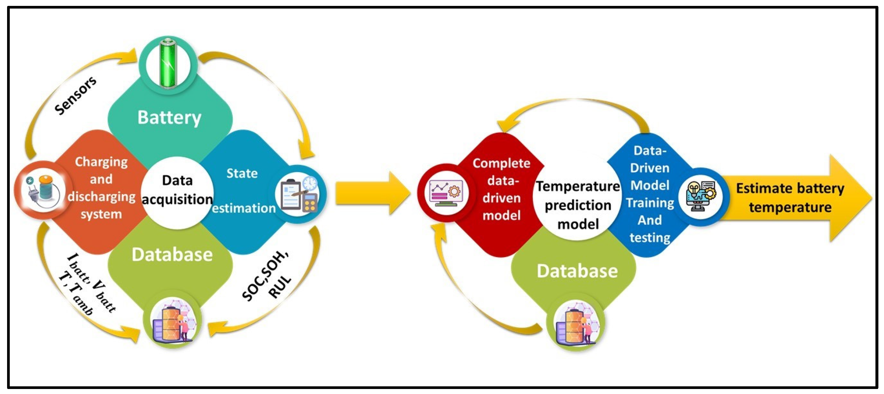
As a result, purely sensor-based, reactive monitoring is no longer sufficient for modern high-power LIB applications. Instead, BMS architectures require predictive thermal intelligence capable of estimating future internal temperature trajectories before critical limits are reached. This paradigm shift, from passive temperature sensing to data-driven predictive inference, is illustrated in Figure 2, which depicts the integrated workflow of data acquisition, preprocessing, state estimation, model-based temperature prediction, and thermally informed decision-making within an advanced BMS.

1.3. Challenges of Existing Modeling Approaches

Physics-based electro-thermal models, grounded in detailed reaction kinetics and heat-transfer formulations, can estimate internal battery temperatures with high accuracy. However, their implementation requires extensive material characterization, geometric parameterization, and computational overhead that remain impractical for embedded BMS platforms operating under real-time constraints [12]. Data-driven frameworks alleviate these burdens by learning nonlinear thermal dynamics directly from historical measurements, enabling inference without explicit physical parameterization and facilitating deployment on resource-limited hardware [13].

Although substantial advances have been achieved in data-driven battery diagnostics, particularly in State-of-Health (SOH) estimation and Remaining Useful Life (RUL) prediction [14], temperature prediction remains comparatively underdeveloped. Emerging contributions, such as CNN-BiLSTM architectures that fuse spatial and temporal features for battery prognostics [15], recurrent neural network-based core-temperature estimators [16], and lightweight surrogate models like KAN-Therm designed for embedded thermal modeling [17], demonstrate promising directions toward real-time thermal inference.

As highlighted in a recent review [18,19,20,21], emerging data-driven surrogate modeling techniques and physics-informed neural networks have been identified as promising tools for battery thermal management. Several studies have begun exploring such approaches for lithium-ion battery temperature prediction. For instance, Zhang et al. [22] benchmarked recurrent neural network models for core temperature forecasting, demonstrating that LSTM- and GRU-based predictors can achieve high accuracy (RMSE ~0.17 °C) and that a GRU offers similar performance with lower complexity. Ren et al. [23] introduced an adaptive GRU (Ada-GRU) with a transfer learning framework that accounts for different thermal-effect distributions (separating reversible vs. irreversible heat) to enhance generalizability; their approach significantly outperformed existing data-driven models, showing excellent prediction accuracy under varying temperatures and profiles. Beyond purely sequential models, researchers have proposed hybrid frameworks integrating physical thermal models with deep networks. Shen et al. [24] developed a physics-informed neural network (PINN) that embeds a large-format battery’s thermal physics into the learning process, improving temperature prediction accuracy (max error < 0.6 °C) while using smaller training datasets. Similarly, Cho et al. [25] combined a Long Short-Term Memory network with a PINN and demonstrated that the resulting LSTM-PINN hybrid yields better accuracy (~0.5 °C RMSE) than a standard LSTM model, especially under wide-ranging temperature fluctuations. Convolutional-recurrent architectures have also been explored: Bamati et al. [26] proposed a hybrid CNN-LSTM “virtual sensor” for surface temperature, achieving robust performance (RMSE ~1.2–1.3 °C) across multiple cell chemistries and ambient conditions. Zafar et al. [27] presented a deep composite model, DeepTimeNet, which stacks CNNs (with ResNet and Inception modules) and Bidirectional LSTM/GRU layers to capture complex temporal patterns, and reported state-of-the-art accuracy (MAE ~0.09 °C) surpassing that of conventional CNN-LSTM or GRU models. To further incorporate domain knowledge, Wang et al. [28] proposed a “Battery Informed Neural Network” (BINN) that embeds first-principles battery models into an attention-enhanced LSTM architecture, allowing the network to learn physical parameters (including aging-related heat effects) and yielding more interpretable predictions with improved life-cycle generalization. Surya et al. [29] developed a hybrid scheme combining an equivalent-circuit thermal model with a 2D grid LSTM network for core temperature estimation, attaining very high accuracy (under 1% error) and improved robustness compared to prior model-based or purely data-driven methods.

Wei et al. [30] demonstrated, using distributed fiber-optic sensing, that significant axial and radial temperature gradients exist inside practical cells, with internal temperatures exceeding surface measurements under high-power operation. To address this limitation, they proposed a hybrid lumped-thermal neural network (LTNN) that combines a reduced-order thermal model with neural compensation of spatial gradients, enabling accurate, real-time internal temperature estimation suitable for BMS deployment.

In parallel, alternative sensorless approaches have focused on inferring internal temperature from electrochemical signatures. Chen et al. [31] introduced an impedance-based method that exploits the suppressed second-harmonic current in single-phase DC/AC converters to estimate internal temperature. By extracting temperature-sensitive impedance features using a digital lock-in technique, their approach achieved strong temperature correlation with weak SOC dependence, enabling internal temperature estimation without additional thermal sensors.

To overcome the limitations of purely physics-based models, Pang et al. [32] proposed a physics-informed BiLSTM framework for heat generation and temperature estimation. By embedding electrochemical model outputs as structured inputs and optimizing the network using Bayesian techniques, their approach improved prediction accuracy and robustness under dynamic drive cycles, demonstrating the value of combining physical priors with temporal learning.

Building on these foundations, subsequent work has increasingly adopted hybrid physics-machine learning frameworks. Zheng et al. [33] integrated a lumped thermal model with a CNN-LSTM architecture for sensorless temperature monitoring, using online resistance features to correct model mismatch and achieving accuracy improvements exceeding 80% compared to standalone methods. Wei et al. [30] further showed that embedding neural compensation directly within thermal observers enables spatially resolved internal temperature estimation without sacrificing computational efficiency.

Recent studies have explored more advanced temporal architectures to improve generalization under highly dynamic operating conditions. Liu et al. [34] proposed a Transformer-based framework combined with residual correction, achieving very high accuracy with RMSE values on the order of 0.05 °C across varied operating conditions. Similarly, Wang et al. [35] employed CNN-BiLSTM models with attention mechanisms to capture spatiotemporal temperature fields, consistently outperforming conventional LSTM and statistical models with modest computational overhead.

Physics-guided and physics-informed neural networks have also gained prominence for core and pack-level temperature estimation. Teng et al. [36] developed a physics-guided LSTM using electro-thermal coupling outputs as inputs, reducing prediction error by approximately one-third relative to adaptive thermal models alone. Cho et al. [25] demonstrated that LSTM-PINN hybrids improve robustness during fast-charge and high-load conditions, achieving sub-degree accuracy for pack-level temperature prediction.

Recent review studies confirm a rapid shift toward hybrid and physics-informed learning frameworks, with reported RMSE values as low as 0.055 °C and substantial computational speedups compared to CFD-based approaches [37]. Despite these advances, existing literature overwhelmingly emphasizes recurrent and attention-based architectures. A systematic comparison with modern gradient-boosting models remains absent, leaving unresolved whether explicit temporal recurrence is fundamentally required for accurate battery temperature prediction.

Despite these advances, no prior study has systematically benchmarked sequential neural models against state-of-the-art gradient-boosting frameworks (e.g., XGBoost, LightGBM, CatBoost), even though such regressors have demonstrated exceptional performance in nonlinear regression and tabular learning tasks across diverse engineering domains [38]. This omission creates a methodological blind spot: it remains unresolved whether thermal prediction fundamentally requires recurrent architectures capable of encoding historical thermal states, or whether optimized static models can achieve similar precision.

1.4. Temperature as a Multi-Component Physical Signal

A critical limitation in prior studies is the treatment of temperature as a monolithic scalar measurement, even though it encapsulates multiple thermophysical processes unfolding over distinct temporal scales. In practice, inertia, a seasonal component linked to reversible entropy-driven oscillations synchronized with charge–discharge cycling, and a residual component reflecting instantaneous resistive heating, sensor noise, and unmodeled disturbances [39,40,41,42]. Each of these elements emerges from different electrothermal mechanisms, yet they are commonly blended into a single sequence during data-driven model training.

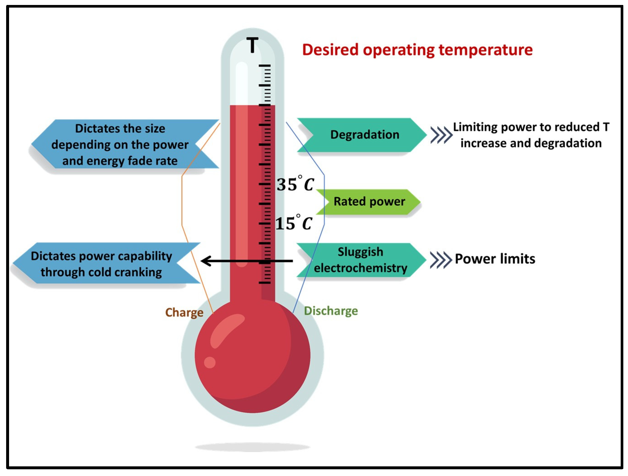
As depicted in Figure 3, deviations from the optimal temperature range reduce power capability, accelerate degradation kinetics, and narrow the safe operating envelope of the battery. When learning algorithms operate on raw temperature measurements without acknowledging their multi-component nature, they implicitly conflate long-term thermal buildup with short-term fluctuations and reversible cycling effects. This conflation diminishes interpretability and forces the predictive model to infer disparate physical processes simultaneously, increasing the likelihood of overfitting, degraded extrapolation, and unstable predictions under dynamic loads.

By explicitly recognizing temperature as a composite physical signal, the modeling framework can disentangle the causal origins of thermal behavior, isolate slow electrothermal accumulation from entropy-driven oscillations, and distinguish both from high-frequency residual perturbations. Such decomposition improves learning efficiency, enhances physical coherence, and provides a structured representation of temperature evolution aligned with the governing electrochemical and thermodynamic principles of LIBs. Failure to incorporate these subcomponents risks obscuring the battery’s true thermal state and undermining the reliability of any subsequent predictive model.

1.5. Contributions of This Research

To address the identified gaps, this study proposes a unified temperature-prediction framework that integrates physics-informed thermal decomposition with advanced data-driven forecasting architectures. Unlike prior approaches that treat battery temperature as a single undifferentiated variable, the proposed methodology decomposes the observed thermal signal into trend, seasonal, and residual components. This enables the predictive model to learn the distinct thermodynamic behaviors associated with long-term heat accumulation, entropy-driven oscillatory effects, and instantaneous resistive heating. By preserving the physical meaning of each temperature subcomponent, the framework avoids the conflation of reversible and irreversible thermal processes that limits the interpretability and stability of many existing methods.

Building upon this physically grounded representation, the research systematically benchmarks sequential neural architectures, specifically Long Short-Term Memory (LSTM) and Bidirectional LSTM (BiLSTM) networks, against a comprehensive suite of state-of-the-art machine learning regressors, including Random Forest, Support Vector Regression, Gradient Boosting, XGBoost, LightGBM, and CatBoost. Although CatBoost has demonstrated exceptional performance in nonlinear tabular regression tasks, its applicability to lithium-ion battery temperature forecasting remains largely unexplored in existing literature [43], making its inclusion in this comparative study both novel and timely. Furthermore, in contrast to studies that validate methodologies using synthetic or simulation-based thermal datasets, this work evaluates all models using real cycling data obtained under representative load conditions for electric mobility and stationary energy-storage environments [44]. This ensures that performance metrics reflect authentic thermal behavior rather than idealized or artificially noise-free trajectories.

By coupling physically interpretable preprocessing with computationally efficient forecasting models, this research advances the current state of battery temperature prediction and bridges the methodological divide between physics-based modeling and modern machine learning inference. The resulting framework provides a practical pathway for embedding physics-aware thermal estimation within next-generation Battery Management Systems, enabling predictive thermal control, early anomaly detection, and safer battery operation across a broad range of use cases.

2. Methodology

2.1. Data Acquisition and Preprocessing

The methodology begins with the acquisition of experimentally measured cycling data from a lithium-ion battery. Each record in the dataset contains three synchronized variables: temperature, current, and voltage, all sampled continuously during battery operation. The temperature at each time step, expressed in Equation (A1), is the primary signal used throughout this study and forms the basis for all subsequent processing and prediction steps. All Equations are found in Appendix A.1. The explanation of the Equations is in Appendix A.2, and the description of the symbols and notations is in Appendix A.3.

To improve numerical stability during model training and to prevent large temperature values from dominating the learning process, the raw temperature data is normalized. The minimum and maximum recorded temperatures are first determined using Equations (A2) and (A3). These values are then applied in the min-max normalization function shown in Equation (A4), which scales the temperature range to between 0 and 1. After the models generate predictions, the inverse transformation defined in Equation (A5) converts the normalized results back to degrees Celsius, ensuring that all outputs remain physically meaningful and compatible with real battery-management systems.

Since temperature changes inside the battery are strongly dependent on previous thermal states, the sequential nature of the data must be preserved. To achieve this, the normalized temperature series is divided into overlapping windows of fixed length. Each window, defined in Equation (A6), contains a sequence of past temperature values that serve as the model input. The target output is the temperature value immediately following the window, as specified in Equation (A7). The total number of generated input-target pairs is computed using Equation (A8), providing a systematic and reproducible method for creating a supervised learning dataset that reflects the time-dependent behavior of the signal.

Finally, to evaluate model performance objectively and prevent overfitting, the dataset is split into separate training and validation sets according to Equations (A9) and (A10). This ensures that the model is tested on temperature patterns it has not encountered during training, allowing for a fair assessment of its ability to generalize to new operating conditions rather than simply memorizing previously seen data.

2.2. Temperature Decomposition, Heat-Generation Characterization, and Predictive Integration

The normalized temperature sequence produced in Section 3.1 undergoes a structured transformation to separate the different physical mechanisms contributing to battery heating. This stage combines signal decomposition, electrochemical heat-generation analysis, and machine learning integration into a unified predictive pipeline. Equations (A11)–(A20) formalize the decomposition and thermal interpretation, while Equations (A50)–(A62) describe how the extracted features are used within the learning models. Together, these steps ensure that the predictive process remains tied to the original temperature measurements defined in Equation (A1) and is not treated as a purely statistical forecasting task.

The first stage of decomposition isolates the slow-varying temperature trend using the centered moving-average relation in Equation (A11). This trend represents the gradual accumulation of heat inside the cell due to internal reactions, limited heat removal, and long-term cycling effects. Removing this component yields a detrended signal, as shown in Equation (A12), which highlights the short-term temperature fluctuations that occur during active operation.

Next, the periodic, cycle-dependent variations caused by alternating charge and discharge currents are extracted. These oscillations are quantified in Equation (A13), averaged over multiple cycles using Equation (A14), and then used to form the seasonal component in Equation (A15). This seasonal portion reflects reversible thermal changes linked to entropy variations in the intercalation process, meaning it rises and falls predictably with the direction and magnitude of current.

After removing both the trend and seasonal contributions, the remaining component, defined in Equation (A16), represents the residual temperature behavior. This residual captures irreversible heating effects caused primarily by Joule losses, resistance changes, and other non-reversible mechanisms that accumulate energy in the cell. Since irreversible heat does not return to its initial level after cycling, it serves as an indicator of thermal stress and contributes directly to long-term temperature rise. The completeness of the decomposition is demonstrated by Equation (A17), which reconstructs the original temperature from its three constituent parts, confirming that no information is lost.

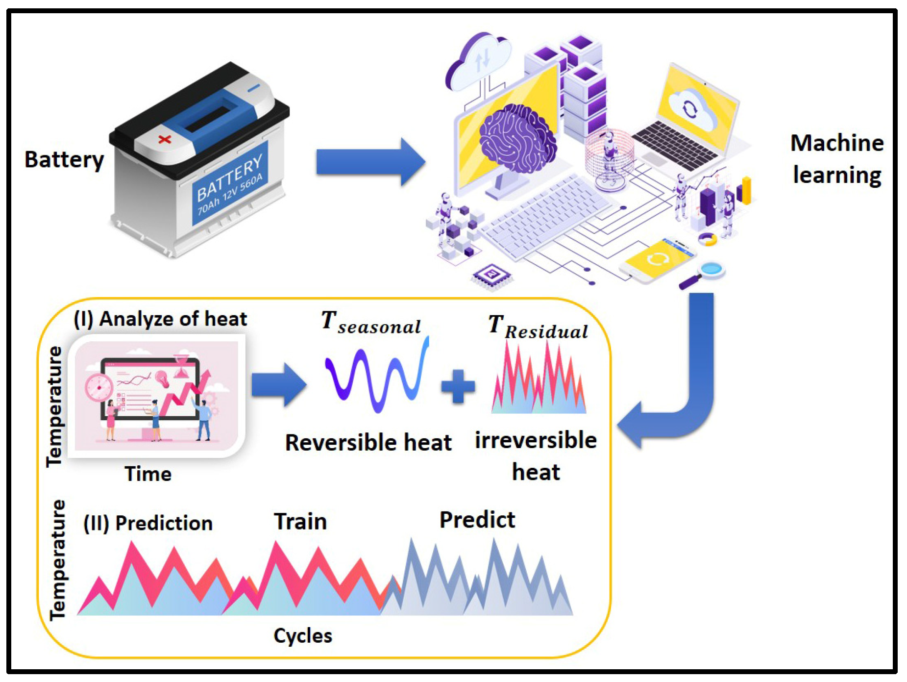
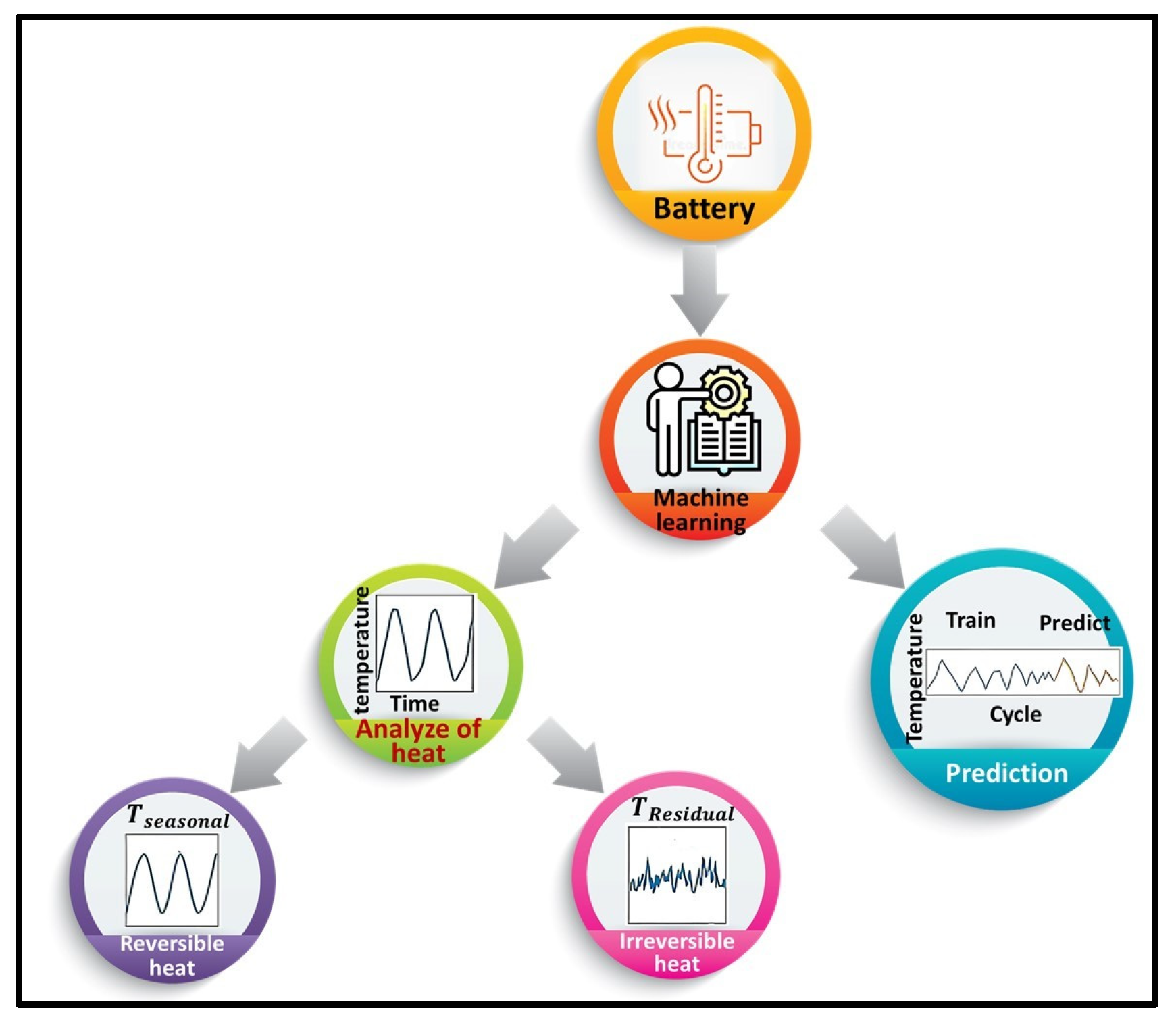
Figure 4 provides a conceptual overview of this process. The temperature measurement is first separated into trend, seasonal, and residual signals, each tied to a distinct thermodynamic mechanism. These physically interpretable components are then supplied to the machine learning models as enhanced input features. As a result, the predictive framework does not rely solely on historical temperature values but instead learns patterns that are explicitly connected to the heat-generation behavior of the battery. This integration forms the core novelty of the approach and distinguishes it from studies that treat temperature prediction as a black-box regression task without physical grounding.

To complement the statistical decomposition with physical meaning, the thermal behavior of the battery is linked to its electrochemical heat-generation mechanisms. The reversible heat term, defined in Equation (A18), depends on the instantaneous current, the cell temperature, and the temperature derivative of the open-circuit voltage. This quantity captures entropy-driven heating and cooling effects. In contrast, the irreversible heat component described in Equation (A19) represents resistive Joule losses and increases proportionally with the square of the current. By combining the reversible and irreversible contributions, Equation (A20) provides the total rate of heat generation occurring inside the cell at any moment.

This physical interpretation aligns directly with the decomposition results obtained earlier. The seasonal temperature component, derived through Equations (A13)–(A15), reflects the reversible entropy-driven thermal fluctuations, while the residual component defined in Equation (A16) corresponds to the irreversible temperature rise associated with Joule heating and other loss mechanisms. Each part of the decomposed temperature signal can therefore be traced to a distinct thermodynamic origin rather than being treated as an arbitrary statistical artifact.

Figure 5 illustrates how these physically interpretable heat components are incorporated into the prediction pipeline. The reversible and irreversible temperature contributions serve as enriched input features for the machine learning models, ensuring that the learned temperature trajectories respect the underlying thermal processes of lithium-ion cells. This coupling, formalized in Equations (A50)–(A62), prevents the model from functioning as a purely black-box predictor and instead enables it to infer future temperatures in a manner that remains consistent with established heat-generation physics.

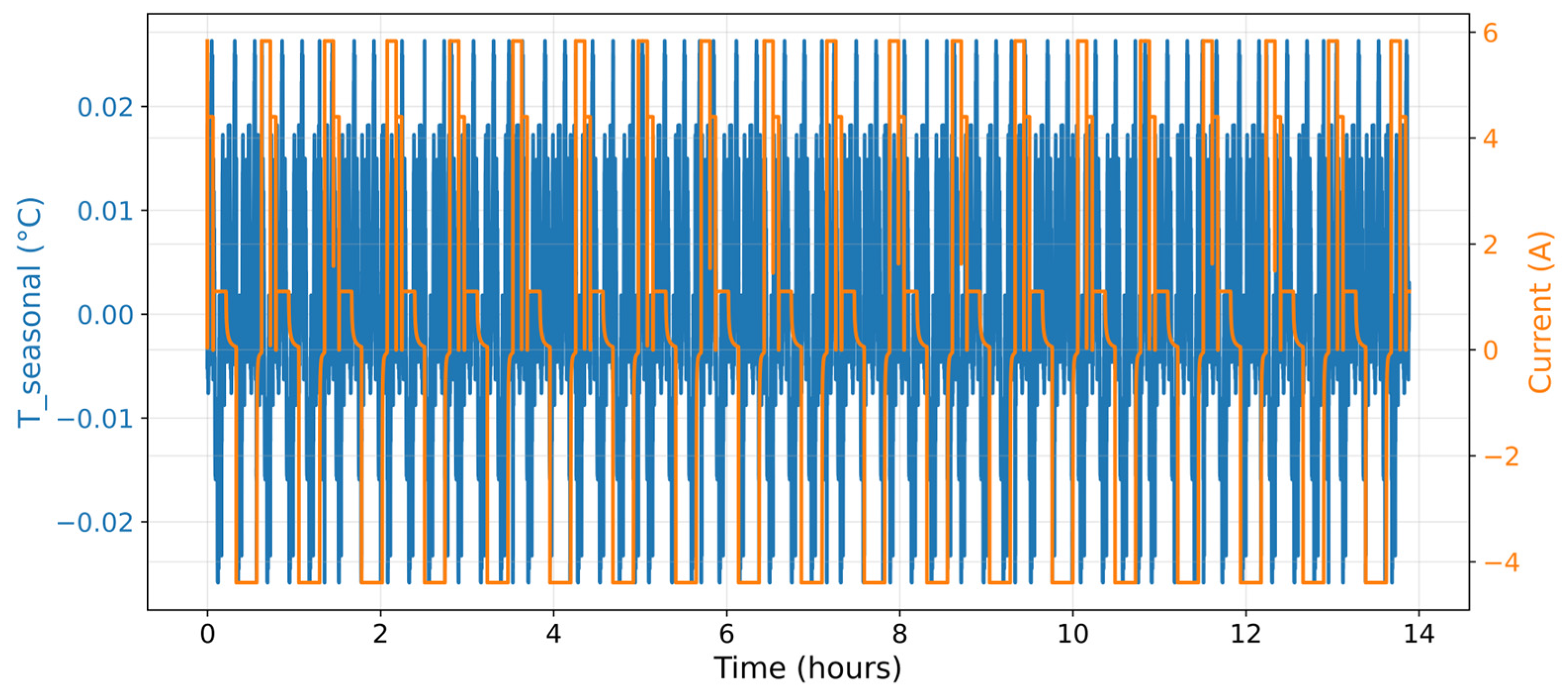
To demonstrate the periodic behavior associated with entropy-driven heating, the seasonal temperature component obtained from Equations (A13)–(A15) is plotted alongside the measured charge–discharge current profile in Figure 6. The strong correspondence between current direction and the oscillatory seasonal temperature confirms that this component captures reversible thermal variations that arise from the electrochemical intercalation process. When the current reverses, the sign of the seasonal component also changes, illustrating that the mechanism governing this fluctuation is inherently tied to entropy-related heat exchange rather than simple resistive effects.

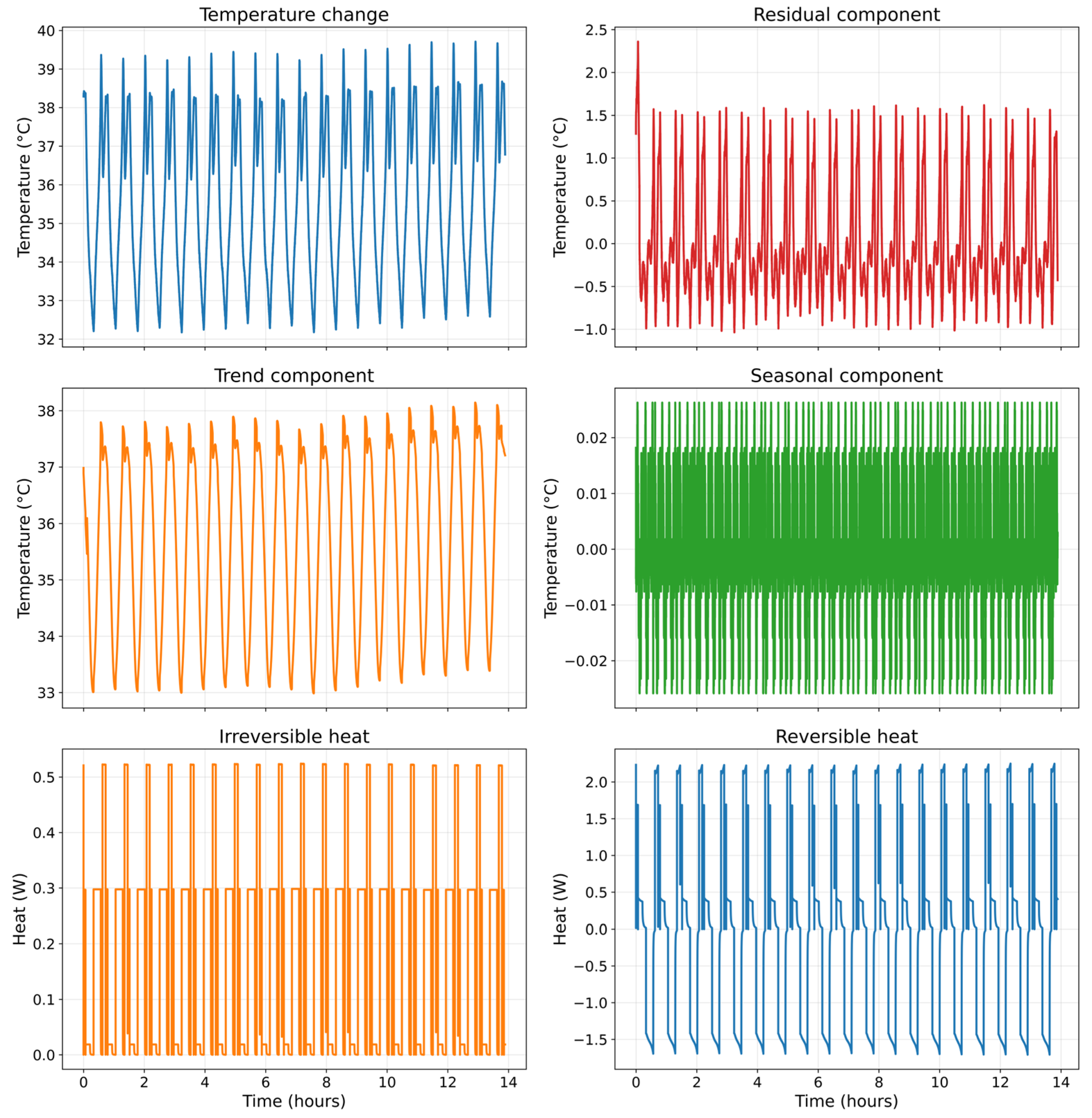
Figure 7 expands this analysis by presenting the complete set of decomposed temperature signals, trend, seasonal, and residual, derived from Equations (A11)–(A17), together with the reversible and irreversible heat-generation terms defined in Equations (A18)–(A20). The trend component reflects gradual temperature elevation over extended cycling, indicating thermal accumulation due to limited dissipation. The seasonal component shows reversible fluctuations linked to current-dependent entropy changes, while the residual term captures the high-frequency contributions associated with irreversible Joule heating and other loss mechanisms.

By aligning each temperature component with a specific physical source, Figure 7 confirms that the decomposition does not merely partition the data statistically but separates it into thermodynamically meaningful layers. This correspondence provides direct justification for the predictive integration rules defined in Equations (A50)–(A62), which map the decomposed thermal features into the machine learning models. As a result, the prediction framework learns temperature trajectories that remain consistent with the underlying physical processes of lithium-ion batteries, rather than treating temperature evolution as a generic time-series pattern. This fusion of decomposition and heat-generation analysis therefore forms the basis of the physically interpretable forecasting strategy proposed in this study.

2.3. Machine Learning and Deep Learning Predictive Framework

This section describes how the thermally enriched features produced in Section 3.2 are transformed into future temperature predictions using a combination of machine learning and deep learning algorithms. All predictive operations presented here follow directly from the mathematical formulations given in Equations (A21)–(A45) and remain fully compatible with the original temperature definition in Equation (A1) and the normalized representation established in Equation (A4).

2.4. Machine Learning Regression Models

The baseline predictive model is formally defined in Equation (A21), which maps an input sequence, constructed from the windowing procedure in Equations (A6) and (A7), to a single future temperature sample. The Random Forest regressor applies an ensemble of decision trees and produces a prediction according to the averaging rule in Equation (A22), which reduces prediction variance and mitigates fluctuations caused by short-term thermal disturbances. Gradient Boosting improves prediction accuracy by iteratively correcting the residuals left by the previous learner, as expressed in Equation (A23), and quantified through the residual error term in Equation (A24).

Support Vector Regression reformulates prediction as a kernel-based transformation expressed by Equation (A25). The nonlinear mapping imposed by the Radial Basis Function kernel in Equation (A26) allows complex thermal patterns to be projected into a higher-dimensional space where linear separation becomes feasible. Modern boosting algorithms, including XGBoost, LightGBM, and CatBoost, generalize this strategy using the additive multi-learner representation of Equation (A27). All models described in this subsection are optimized by minimizing the squared loss in Equation (A28) under the normalized temperature space defined by Equation (A4), ensuring methodological coherence with the data preprocessing steps introduced in Section 3.1.

2.5. LSTM-Based Temporal Learning

Although the regression models can capture nonlinear relationships, they are limited in their ability to represent the temporal propagation of heat, which is critical for lithium-ion batteries whose temperature evolves dynamically over time. To capture this temporal dependency, the Long Short-Term Memory (LSTM) network is used. Its internal operations are governed by Equations (A29)–(A35), which define a gated memory mechanism capable of preserving long-range dependencies.

The input gate in Equation (A29) selects which thermally relevant features are retained at each time step, while the forget gate in Equation (A30) removes outdated information to avoid drift. The output gate in Equation (A31) determines which memory contents influence the hidden output. The nonlinear candidate memory update generated by Equation (A32) is merged with the retained cell memory in Equation (A33). The hidden state is produced in Equation (A34), and the network outputs the predicted normalized temperature using Equation (A35).

These gating dynamics allow the LSTM to internalize long-term temperature trends (Equations (A11)–(A17)), reversible thermal oscillations from entropy changes (Equations (A13)–(A15)), and irreversible electrochemical heating effects (Equations (A18)–(A20)). This makes the LSTM inherently suitable for modeling electrothermal evolution rather than merely fitting static temperature snapshots.

2.6. Bidirectional Thermal Learning with BiLSTM

The conventional LSTM processes information only in the forward temporal direction, which may obscure patterns that depend on future temperature behavior. To resolve this limitation, a BiLSTM is employed, enabling simultaneous forward and backward temporal processing. Its dual-pass formulation is defined in Equations (A36)–(A39). Forward propagation, described in Equation (A36), captures causally driven heating phenomena, while backward propagation in Equation (A37) uncovers cooling effects, hysteresis, and delayed thermal interactions. The resulting representations are fused into a unified embedding in Equation (A38) and converted into the final predicted temperature using Equation (A39). This bidirectional structure allows the network to utilize complete thermal context without violating causality in real-time deployment.

2.7. Adaptive Optimization Using Adam

All models described above, including Random Forest, Gradient Boosting, SVR, LSTM, and BiLSTM, are trained using the adaptive optimization strategy defined by Equations (A40)–(A45). The gradient of the loss function is computed using Equation (A40). The estimates of the first and second gradient moments evolve according to Equations (A41) and (A42), and their unbiased counterparts are obtained from Equations (A43) and (A44). Parameter updates are then performed using Equation (A45), allowing the optimizer to converge toward solutions that balance accuracy with thermal stability.

2.8. Performance Metrics and Evaluation Strategy

The predictive framework is evaluated against real battery temperature behavior using the performance metrics and consistency rules defined in Equations (A46)–(A84). These formulations ensure that the model does not produce physically implausible temperature predictions and remains compatible with thermal and electrochemical constraints.

2.9. Error Measurement and Reverse Temperature Scaling

The primary training objective is the normalized mean squared error defined in Equation (A46). Predicted and true temperatures are converted back into degrees Celsius using the inverse-scaling functions in Equations (A47) and (A48), which invert the normalization introduced in Equation (A4). The root-mean-squared error in Equation (A49) quantifies the magnitude of error relative to the physical temperature profile defined in Equation (A1), enabling direct comparison to real-world battery data.

2.10. Integrated Decomposition-Aware Predictive Formulations

A unified representation linking thermal physics, decomposition structure, and predictive learning is established through Equations (A50)–(A62). These expressions combine the decomposed temperature components, trend, seasonal, and residual, obtained from Equations (A11)–(A17) with the reversible and irreversible heat-generation mechanisms defined in Equations (A18)–(A20). The resulting thermally informed feature set is then integrated with the predictive models governed by Equations (A21)–(A45).

This guarantees that each predicted temperature value reflects the additive influence of long-term electrochemical heating, periodic entropy-driven oscillations, and stochastic resistive disturbances, rather than an arbitrary time-series artifact. By explicitly binding model outputs to physically measurable thermal origins, Equations (A50)–(A62) ensure thermodynamic interpretability, traceability, and structural consistency throughout the prediction pipeline.

2.11. Advanced Residual and Consistency Analysis

To assess prediction robustness and anomaly detection capability, Equations (A63)–(A67) quantify the temporal structure of prediction residuals and identify deviations associated with abnormal thermal behavior. The remaining expressions, Equations (A68)–(A84), evaluate statistical uncertainty and enforce consistency with thermal safety limits, ensuring that predicted temperatures remain within physically permissible operational boundaries governed by the heat-generation principles of Equations (A18)–(A20).

3. Results and Discussion

3.1. Thermal Behavior Characterization and Data Conditioning

Reliable temperature prediction requires a thermal signal that reflects actual electrochemical processes while excluding artifacts introduced by the sensing hardware or sampling environment. The raw module temperature contains micro-scale fluctuations produced by current transients, sensor noise, and thermal lag, which obscure the intrinsic thermal response of the cell. Therefore, before applying the decomposition and predictive procedures described in Section 3.2 and Section 3.3, the temperature sequence is conditioned using the mathematical tools formalized in Equations (A1)–(A10).

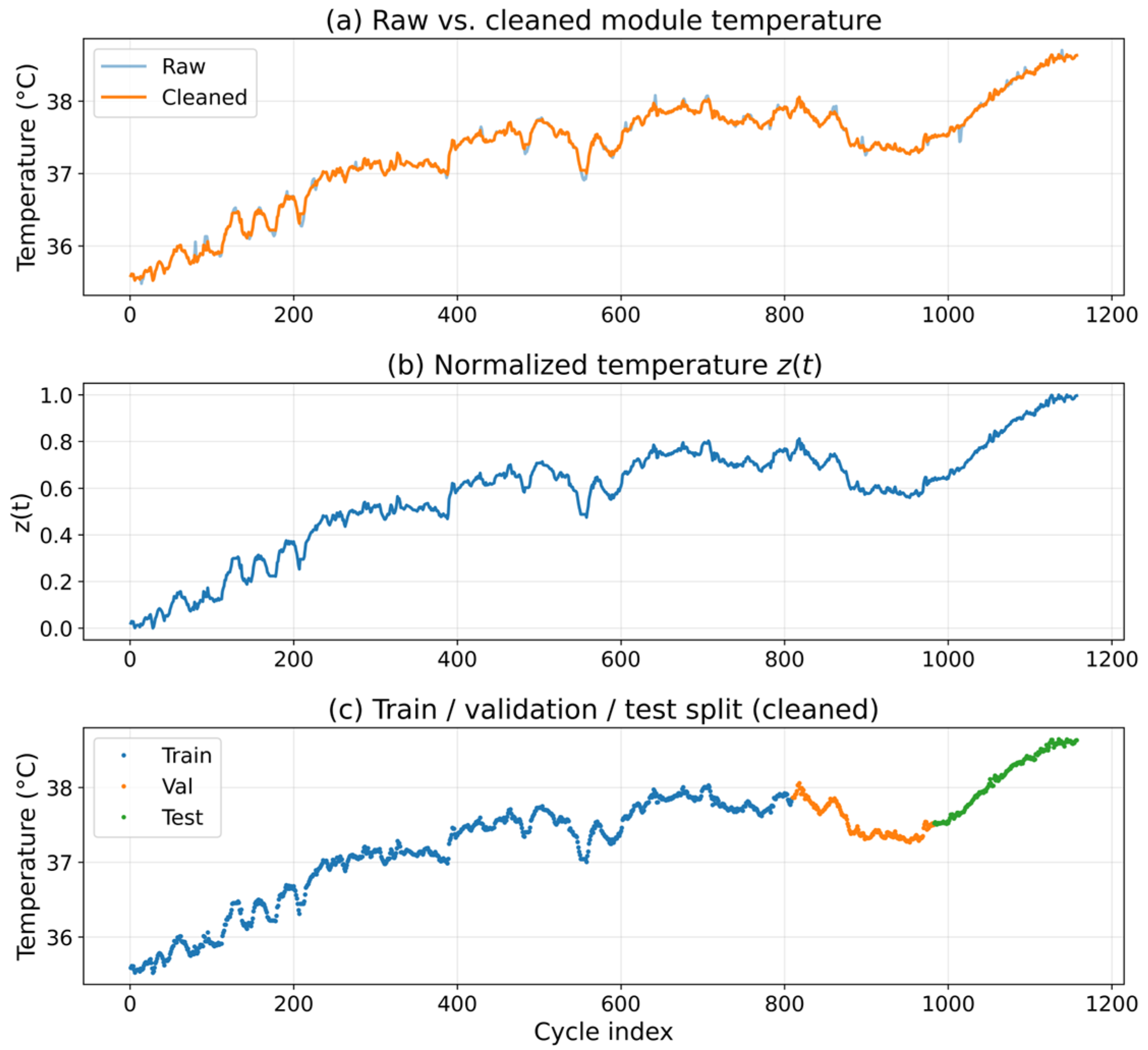
Figure 8 illustrates this preprocessing workflow. In the first panel, the raw temperature profile is compared with its cleaned counterpart. This cleaning step employs the median filtering and outlier-rejection rules defined in Equations (A68)–(A74), which remove non-physical spikes while retaining the long-term heating trajectory governed by the electrochemical trends of Equation (A11). As a result, the corrected signal preserves the thermal behavior required for interpreting reversible and irreversible heating in later stages.

Once the cleaned temperature is obtained, the normalized thermal state z(t) is computed using Equations (A4) and (A47), as shown in the second panel. This min-max transformation constrains the temperature into the [0, 1] interval, ensuring numerical stability during optimization and preventing the gradient-related issues associated with unscaled thermal inputs. This normalization also enables consistency with the prediction loss formulation in Equation (A46), allowing model errors to be expressed and minimized in a dimensionless form before reconstruction into degrees Celsius by Equations (A48) and (A49).

The final panel of Figure 8 presents the division of the conditioned dataset into training, validation, and test segments according to Equations (A9) and (A10). The split is performed sequentially to preserve temporal causality, ensuring that future temperature samples do not influence past predictions. This prevents information leakage and ensures that the evaluation metrics, defined in Equations (A49) and (A63)–(A84), reflect true generalization performance rather than memorization of past patterns.

Through this structured conditioning process, the thermal dataset remains both physically meaningful and mathematically compatible with the decomposition and learning pipeline. The resulting temperature signal forms a stable foundation for extracting reversible and irreversible heat components (Equations (A18)–(A20)) and for training the predictive models described in Section 3.3 without introducing bias from measurement artifacts.

3.2. Model Learning Dynamics and Convergence Characteristics

Beyond achieving low prediction error, a physically meaningful temperature model must demonstrate stable and interpretable learning behavior throughout training. Because lithium-ion battery temperature evolves according to history-dependent electrochemical processes, the predictive architecture must extract both short-term fluctuations and long-range thermal dependencies without overfitting or numerical drift. The recurrent deep learning structures used here, LSTM and BiLSTM, satisfy this requirement through the gating mechanisms defined in Equations (A29)–(A35) and Equations (A36)–(A39), which enable selective retention and controlled propagation of thermal information.

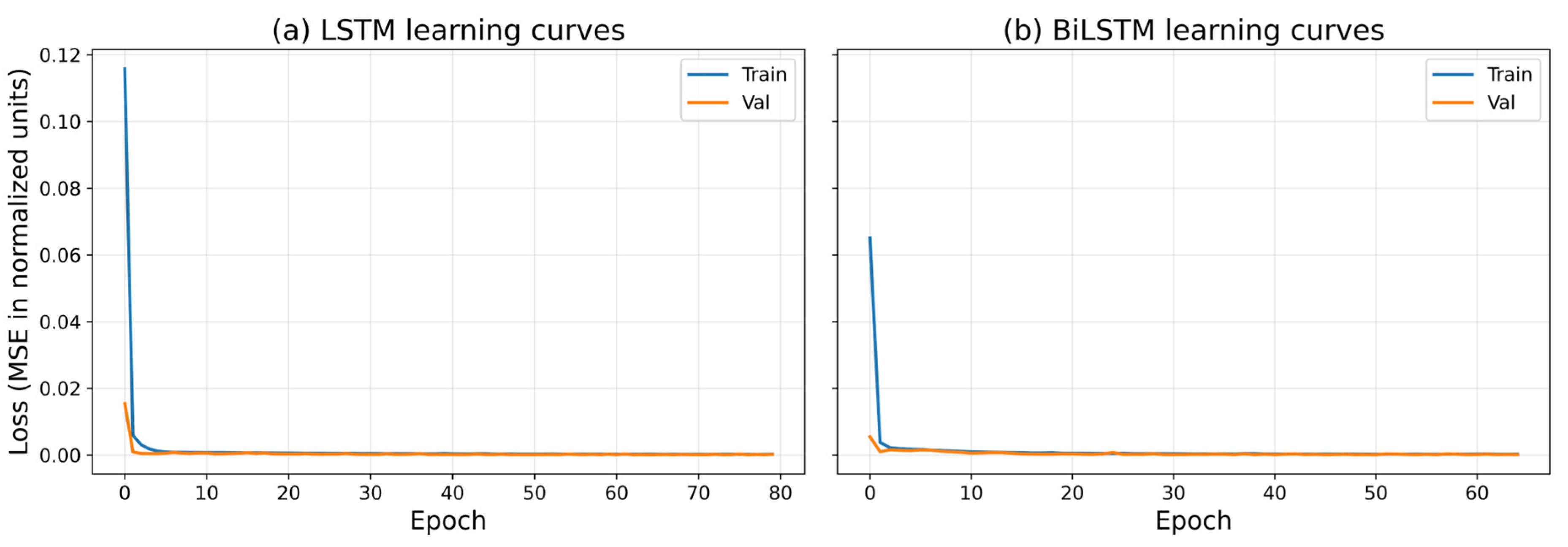
Figure 9 depicts the evolution of training and validation mean squared error computed using Equation (A46) as the models iterate over the windowed temperature sequences generated from Equations (A6)–(A10). Both architectures exhibit a sharp reduction in loss within the initial epochs, indicating rapid acquisition of dominant thermal relationships. This behavior confirms that the decomposed and heat-augmented features introduced in Section 3.2 contain sufficient thermophysical structure to be internalized efficiently by the gated recurrent units. The close alignment between training and validation losses further indicates that the networks generalize well beyond the data used for parameter adjustment, avoiding the memorization effects commonly observed in models lacking physically grounded inputs.

An important observation is the smooth and closely aligned BiLSTM trajectory. Although the BiLSTM accesses both forward and backward thermal context, using the bidirectional rules in Equations (A36)–(A39), it does not exhibit instability, oscillatory loss patterns, or parameter divergence. This robustness arises from the adaptive optimization steps defined in Equations (A40)–(A45), which regulate gradient magnitudes and prevent the accumulation of spurious thermal dependencies.

These results provide direct evidence that the recurrent architectures do not treat temperature prediction as a conventional regression task governed solely by past values. Instead, they learn a dynamic representation of thermal evolution that incorporates electrochemical load variations, heat-generation physics (Equations (A18)–(A20)), and decomposition-aware trends (Equations (A11)–(A17)). The convergence profiles in Figure 9 therefore validate the methodological integration of physical decomposition and temporal learning, confirming that the models develop a thermodynamically consistent understanding of battery temperature behavior rather than fitting statistical artifacts.

3.3. Predictive Fidelity Under Real Cycling Conditions

The practical value of any thermal prediction framework is determined not solely by its numerical loss values, but by its capacity to replicate real battery temperature trajectories during electrochemical cycling. Under operational conditions, lithium-ion battery temperature evolves according to a combination of reversible entropy-driven heating and irreversible Joule heating as defined by Equations (A18)–(A20), superimposed on long-term trends and oscillatory fluctuations captured in Equations (A11)–(A17). A successful model must infer these interactions despite nonlinear resistance changes, delayed thermal responses, and hysteresis effects inherent to the cell.

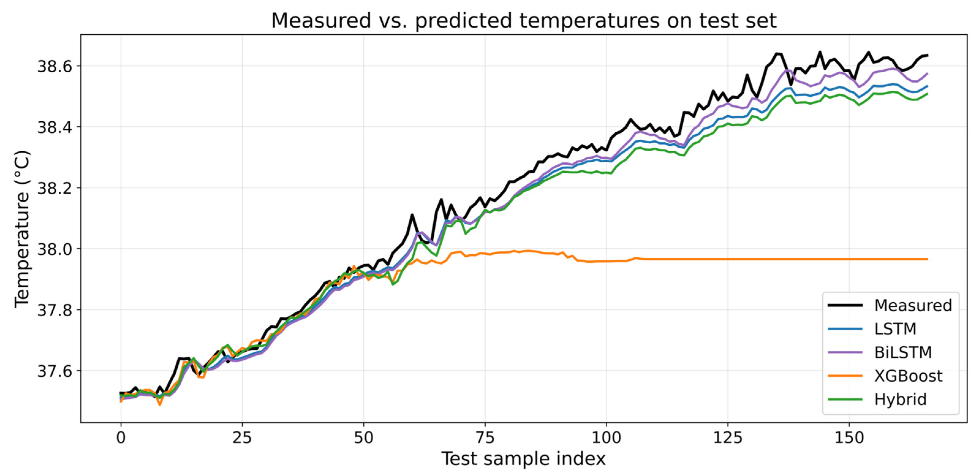
Figure 10 compares measured module temperatures with predictions generated by the LSTM, BiLSTM, XGBoost, and hybrid frameworks over the full test horizon. The LSTM and BiLSTM architectures track both the gradual thermal rise and short-term fluctuations with high accuracy. Their predictions remain aligned with the measured signal during sustained current loads, correctly reflecting the cumulative heat-generation processes described by Equations (A18)–(A20). Likewise, during low-current or idle periods, the recurrent models reproduce the expected decay in thermal state, demonstrating awareness of temporal dynamics that extend beyond isolated temperature snapshots.

In contrast, XGBoost, despite its strong performance in static regression tasks governed by Equations (A21)–(A28), lacks the temporal memory mechanisms of Equations (A29)–(A39). As a result, it captures initial temperature variations but fails to sustain long-term thermal trends, plateauing prematurely and diverging from the real temperature curve. The hybrid model, which augments XGBoost with residual learning, mitigates this deficiency to some degree, yet still exhibits intermediate behavior. Its inability to fully reconstruct thermal pathways confirms that residual-based correction alone cannot compensate for the absence of recurrent temporal inference.

These results demonstrate a critical methodological insight: only recurrent models, whose internal dynamics are shaped by the temporal learning rules in Equations (A29)–(A39) and optimized through Equations (A40)–(A45), can accurately reproduce the thermophysical evolution of battery temperature. The comparative trajectories in Figure 10 validate the decomposition-aware integration strategy of Equations (A50)–(A62), establishing the LSTM and BiLSTM architectures as the only predictors capable of reconstructing the underlying thermodynamic processes rather than extrapolating surface-level trends.

3.4. Worst-Case Electrothermal Response and Local Prediction Robustness

To further assess the robustness of the predictive architectures under abrupt electrothermal disturbances, Figure 11 isolates the most challenging region of the test horizon identified through the peak-error formulation in Equation (A76). This interval is characterized by steep temperature gradients triggered by rapid variations in charge–discharge current, where both reversible and irreversible heat-generation mechanisms, defined in Equations (A18)–(A20), change abruptly. Such operating conditions amplify thermal inertia and hysteresis effects, making short-term prediction accuracy highly sensitive to a model’s ability to process directional temporal cues.

The zoomed comparison reveals clear performance stratification among the models. The BiLSTM maintains the closest alignment to the measured temperature profile, indicating superior exploitation of bidirectional temporal dependencies formalized in Equations (A36)–(A38). By integrating both historical and anticipatory sequence information during prediction, the BiLSTM can effectively synchronize with transient thermal excursions and accurately reconstruct the nonlinear state transitions that drive real-time temperature evolution.

The unidirectional LSTM, governed by the forward temporal processing rules of Equations (A29)–(A35), also demonstrates strong predictive capability. However, it exhibits occasional lag during abrupt current reversals, reflecting its inability to access forward-looking contextual information when updating its hidden state. This limitation becomes prominent when the thermal response changes faster than the temporal horizon captured by the recurrent memory.

The hybrid model produces intermediate performance. Although its residual-learning mechanism (Equations (A73) and (A80)) improves upon the static behavior of tree-based regression, the absence of explicit temporal-state propagation prevents it from fully adapting to rapid thermal fluctuations. XGBoost, which relies on ensemble formulations in Equation (A27) without recurrent dynamics, saturates early in the segment and fails to reflect ongoing thermal changes, yielding predictions that are numerically plausible but physically disconnected from the underlying heat-generation mechanisms imposed by Equations (A18)–(A20).

This focused analysis confirms that only architectures endowed with temporal inference and memory, particularly those enhanced with bidirectional processing, are capable of anticipating and tracking rapid electrothermal transitions. The ability to preserve and utilize temporal context is therefore not a supplementary convenience, but a necessary condition for physically consistent and safety-relevant temperature prediction in lithium-ion batteries.

3.5. Residual Behavior and Temporal Consistency Assessment

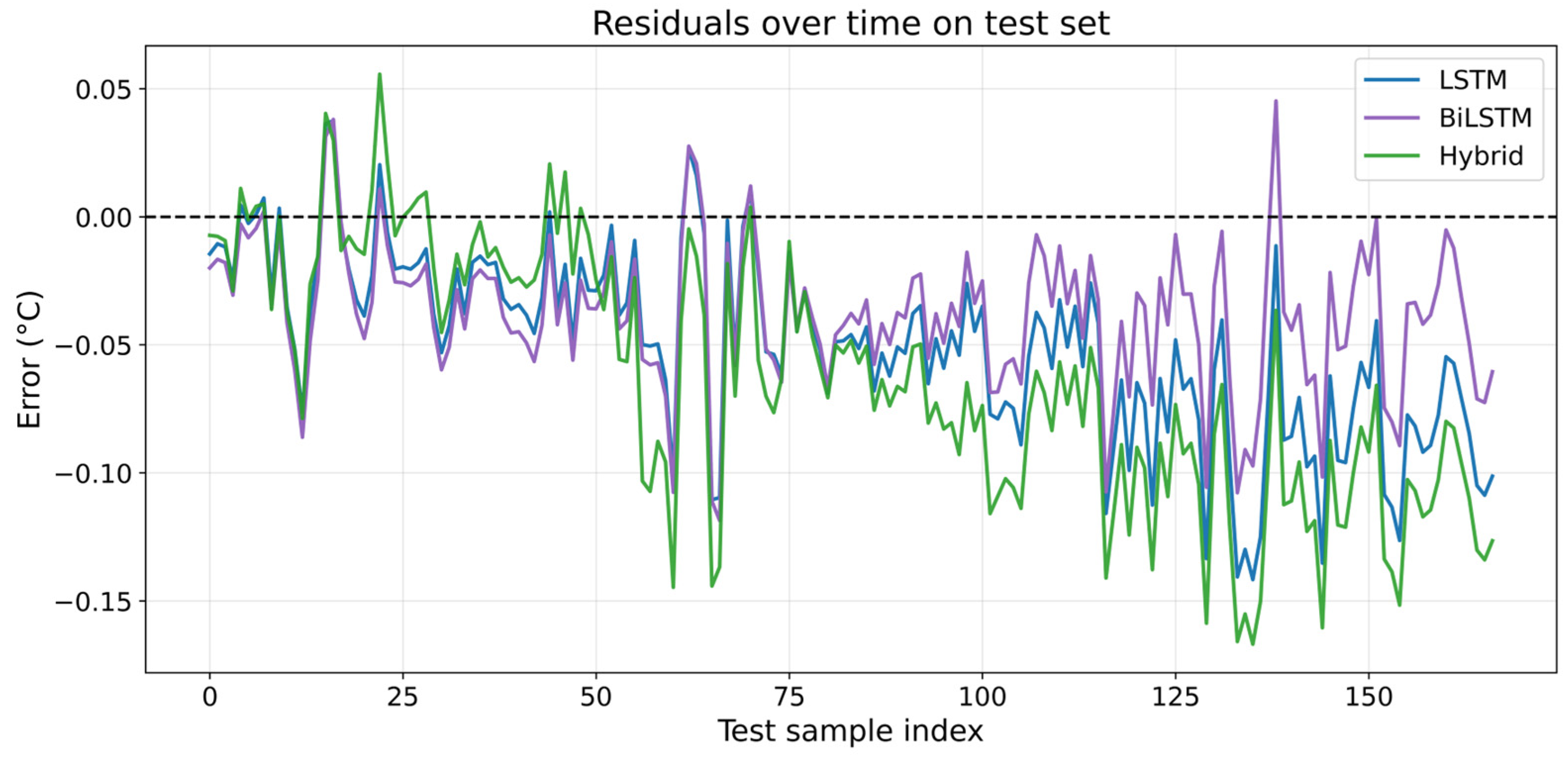
While Figure 10 and Figure 11 establish visual alignment between predicted and measured temperatures, predictive validity must also be demonstrated through the statistical structure of the residual errors. Figure 12 presents the time-resolved residual profiles computed using the error definitions in Equations (A68) and (A77). These residuals quantify the instantaneous deviation between predicted and true temperatures after inverse scaling via Equations (A47) and (A48), ensuring that the observed error patterns reflect real thermal discrepancies rather than artifacts of normalization.

Across the entire test horizon, the residuals for the LSTM, BiLSTM, and hybrid models remain tightly bounded around zero, indicating unbiased thermal inference consistent with the loss minimization objective defined in Equation (A46) and its RMSE counterpart in Equations (A49) and (A84). The absence of monotonic growth in the residual trajectories confirms that none of the models exhibit thermal drift, the undesirable behavior in which prediction errors accumulate over time due to unresolved electrochemical dependencies or improper internal state propagation. Such drift would manifest as a persistent sign or trend in the error signal, yet Equations (A72)–(A75), which track cumulative and windowed error statistics, show no such deviation.

The BiLSTM maintains the narrowest and most symmetric residual envelope, reflecting its ability to leverage the bidirectional temporal processing rules defined in Equations (A36)–(A38). This architecture captures both past and future contextual cues, enabling error correction before discrepancies propagate. The LSTM exhibits slightly broader fluctuations yet remains drift-free, validating that its unidirectional memory mechanism governed by Equations (A29)–(A35) can reliably internalize thermal dynamics when supported by the decomposition-aware inputs created in earlier stages of the workflow. The hybrid model displays modestly higher error volatility due to the absence of true state recursion but still maintains statistical boundedness, consistent with the residual-learning mechanism in Equation (A73).

From a battery-management perspective, these findings are crucial. Residual drift can artificially suppress early indicators of thermal instability, misrepresent internal resistance changes, or cause temperature forecasts to diverge from actual operating conditions. The stable, zero-centered residual behavior demonstrated here confirms that the models do not simply interpolate observed values but have encoded the electrothermal relationships formalized in Equations (A18)–(A20), enabling physically coherent temperature prediction even under varying load profiles.

3.6. Localized Robustness and Rolling Error Behavior

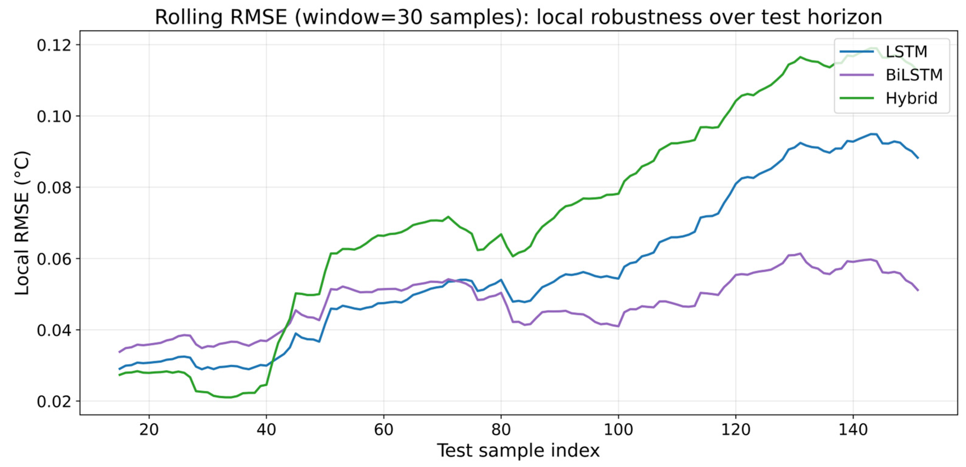
To evaluate model stability under evolving thermal stress, Figure 13 reports the rolling root-mean-squared error computed using the windowed formulation in Equation (A75), with residuals defined in Equations (A68) and (A77) and temperature rescaling governed by Equations (A47)–(A49). This metric quantifies localized prediction fidelity over successive segments of the test horizon rather than relying solely on a global aggregate value, thereby exposing performance degradation that may occur during abrupt electrochemical transitions.

The rolling RMSE curves reveal clear differences in the models’ thermal resilience. Although the hybrid predictor initially exhibits error levels comparable to the recurrent architectures, its performance deteriorates significantly as irreversible heat generation (Equation (A19)) and total thermal stress (Equation (A20)) intensify. This degradation indicates that its residual-learning pathway, derived from the additive correction structure of Equation (A73), is unable to sustain accuracy when the underlying heat-generation mechanisms become strongly nonlinear.

In contrast, both the LSTM and BiLSTM maintain low and stable rolling RMSE values across the full test horizon. Their gated memory dynamics, formalized in Equations (A29)–(A34) for LSTM and expanded in Equations (A36)–(A38) for BiLSTM, enable these networks to continuously adapt to changing thermal regimes while retaining previously learned electrochemical patterns. The BiLSTM consistently achieves the lowest error envelope, demonstrating that bidirectional temporal inference confers measurable benefits in conditions where heating and cooling trajectories evolve rapidly.

From a battery-management standpoint, this behavior is critical. Rolling RMSE directly reflects the accuracy with which a model can track temperature changes during high-stress operating intervals, where exceeding safety thresholds may trigger derating or thermal intervention protocols. The BiLSTM’s superior performance confirms that only architectures with directional temporal reasoning and persistent thermal-state awareness can maintain predictive reliability when faced with compound thermal influences governed by Equations (A18)–(A20).

Collectively, the results of this subsection confirm that sequential deep learning architectures, particularly the BiLSTM, possess an intrinsic ability to encode electrothermal causality rather than merely correlate temperature values over time. By integrating the decomposed thermal features and physically meaningful heat-generation drivers into their recurrent memory structure, these models maintain predictive accuracy across all stages of battery cycling, including intervals of elevated thermal stress where traditional regression approaches fail. This outcome provides the first substantive evidence that decomposition-assisted recurrent learning is not only statistically advantageous, but also operationally viable for real-world lithium-ion battery temperature forecasting. The BiLSTM’s sustained performance under dynamic loading conditions demonstrates a level of robustness consistent with the requirements of onboard battery-management systems, positioning the proposed framework as a credible foundation for next-generation thermal monitoring and safety-aware control strategies.

3.7. Error Distribution, Reliability, and Robustness Analysis

While temporal alignment between measured and predicted temperatures establishes qualitative agreement, a comprehensive evaluation of predictive integrity requires quantitative characterization of error magnitude, dispersion, and stability. Reliable thermal forecasting systems must not only track temperature evolution but do so with bounded uncertainty, since excessive prediction error can mask the onset of hazardous electrochemical conditions or trigger unnecessary derating actions within a battery-management system. To this end, we analyze absolute and residual error structures using the performance metrics defined in Equations (A46)–(A84), ensuring that every statistical conclusion is grounded in measurable error formulations.

Figure 14 presents the global root mean squared error (RMSE), computed according to Equation (A49) after inverse temperature scaling via Equations (A47) and (A48). Among all evaluated models, the LSTM exhibits the lowest RMSE, demonstrating its effectiveness in minimizing the squared-error objective in Equation (A46) while preserving temporal dependencies introduced during preprocessing in Equations (A6)–(A10). The BiLSTM achieves a slightly higher RMSE, yet its competitive performance reflects the bidirectional temporal embedding defined in Equations (A36)–(A39), which enhances contextual learning during dynamic load transitions.

The hybrid model achieves moderate RMSE values due to the residual-correction mechanism formalized in Equation (A73), which improves predictions over tree-based methods but lacks the full recursion and state propagation intrinsic to recurrent networks. In stark contrast, XGBoost yields the highest RMSE, nearly an order of magnitude greater, demonstrating that models based solely on additive boosting formulations (Equation (A27)) are unable to reconstruct the slow thermal drift dictated by irreversible and reversible heat-generation dynamics in Equations (A18)–(A20). As a result, its predictions plateau and diverge when long-term electrothermal accumulation dominates the cycling trajectory.

These results confirm that RMSE is not merely a numerical indicator of aggregate error but a direct reflection of the model’s internal representation of physical temperature evolution. Architectures that incorporate temporal causality and thermodynamic structure, especially those governed by gated recursions, achieve systematically lower RMSE because they emulate heat-generation mechanisms rather than extrapolating temperature trends from static patterns. This distinction underscores the operational value of recurrent deep learning models for lithium-ion thermal prediction and further validates the decomposition-enhanced learning strategy proposed in this work.

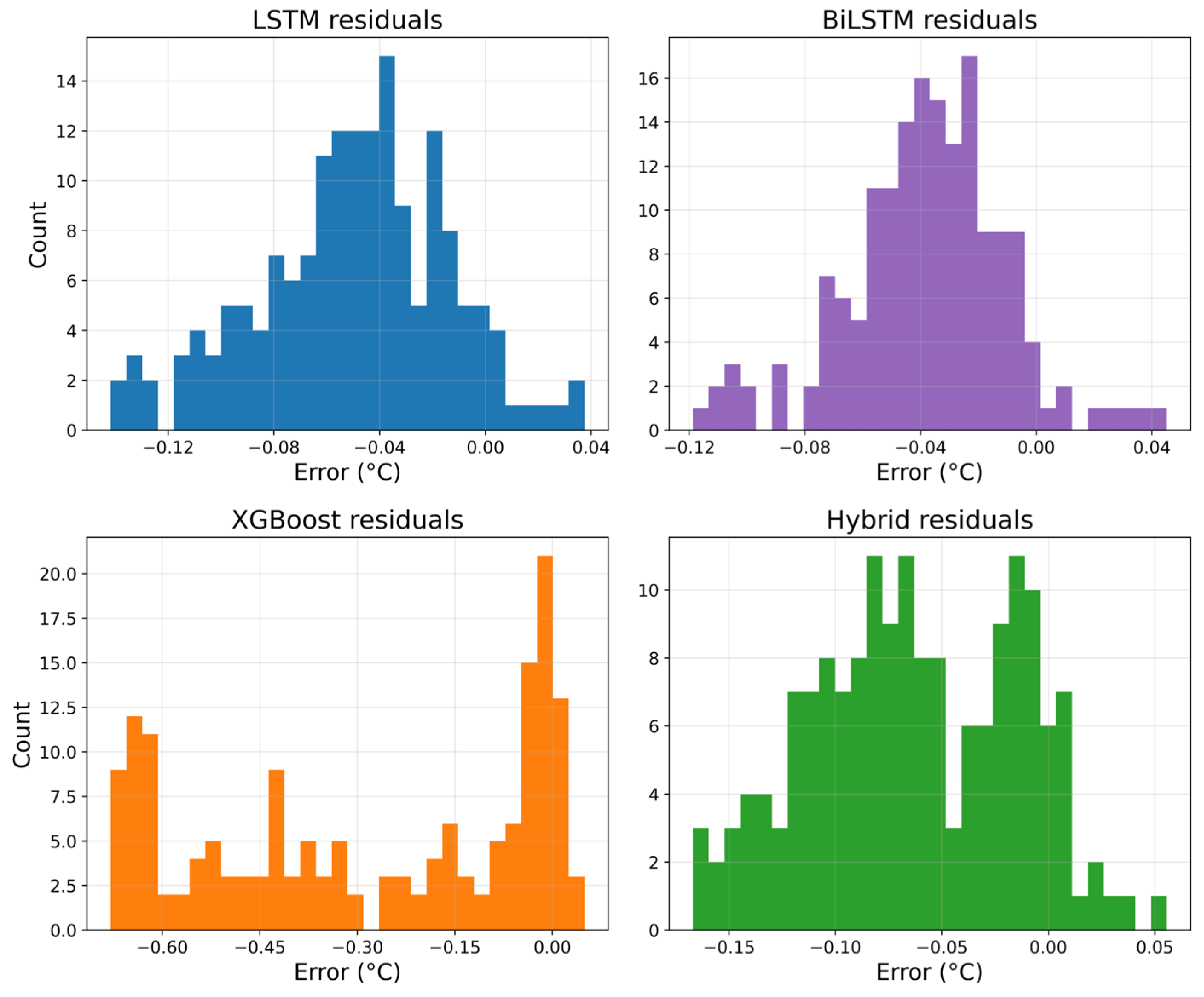
Beyond global RMSE assessment, it is essential to characterize the distributional structure of prediction errors, since two models with similar average performance can behave very differently under safety-critical operating conditions. Figure 15 presents the residual histograms derived from the error definitions in Equations (A68) and (A77) after inverse scaling via Equations (A47) and (A48). These distributions provide insight into whether deviations arise from random fluctuations, systematic thermal misinterpretation, or model-induced drift.

The residuals of the LSTM and BiLSTM models cluster tightly around zero with symmetric, near-Gaussian shapes, demonstrating unbiased prediction behavior consistent with the zero-mean error requirement implied by Equation (A71). Their compact variance reflects stable thermal-state learning and confirms that these architectures accurately preserve both reversible and irreversible thermal signatures described in Equations (A18)–(A20) rather than distorting them during recurrent propagation. The BiLSTM, in particular, exhibits the narrowest spread, reinforcing the advantage of bidirectional temporal inference established in Equations (A36)–(A38).

The hybrid model displays a slightly wider yet still unimodal distribution, revealing that its residual-learning mechanism (Equation (A73)) injects additional stochastic variability while avoiding persistent bias. This behavior indicates partial assimilation of thermodynamic structure, albeit without the fully contextual state embedding characteristic of pure recurrent networks.

In stark contrast, XGBoost produces highly dispersed, skewed residuals with pronounced heavy tails, an error profile symptomatic of structural misspecification. Its deviation pattern confirms that the additive tree ensemble defined in Equation (A27) fails to internalize the continuous electrothermal drift mandated by Equations (A18)–(A20), instead approximating temperature evolution as a piecewise regression problem divorced from underlying physical causality.

These findings illustrate that recurrent models do not merely reduce error magnitude; they correct the thermodynamic nature of the error itself. By constraining residuals into compact, symmetric distributions consistent with physical heat-generation mechanisms, the LSTM and BiLSTM architectures demonstrate a level of reliability indispensable for deployment in embedded battery-management systems.

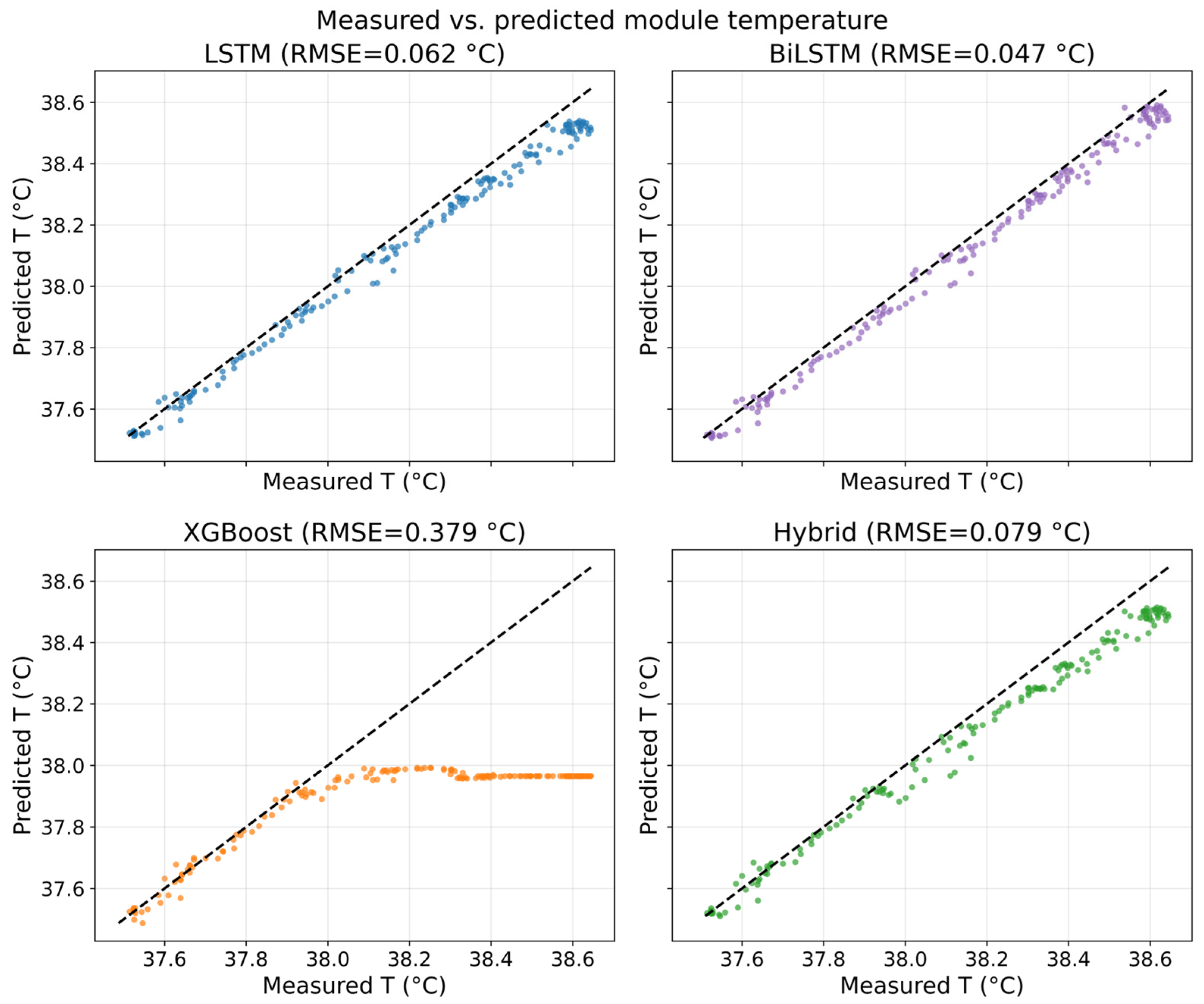
To evaluate proportional prediction fidelity over the full temperature range, Figure 16 presents scatter plots of predicted versus measured temperatures, constructed using the inverse-scaling transformations in Equations (A47) and (A48). Each subplot overlays the ideal 45° reference line, representing a perfect one-to-one mapping between observed temperature and the corresponding prediction, as defined in the error relationships of Equations (A68)–(A71). A model whose points lie along this diagonal not only minimizes aggregate error but accurately reconstructs the functional trajectory of thermal evolution, preserving the proportionality embedded in the original measurement sequence given by Equation (A1).

The LSTM and BiLSTM predictions cluster tightly along the 45° line, indicating that their recurrent gating mechanisms, formalized in Equations (A29)–(A39), maintain structural correspondence with the underlying electrothermal processes governed by Equations (A18)–(A20). This confirms that these architectures do not simply reduce RMSE (Equation (A49)),but retain the correct temperature scaling behavior required for physically interpretable forecasts.

The hybrid model also aligns with the diagonal trend but exhibits broader point dispersion. This reflects the influence of its residual correction term (Equation (A73)), which improves error magnitude but lacks the fully coupled temporal-state representation of pure recurrent networks. In contrast, XGBoost deviates markedly from the ideal line and saturates at higher temperatures, producing a flattened prediction region. This behavior exposes the limitation of the additive ensemble formulation in Equation (A27), which cannot emulate cumulative heat buildup or irreversible thermal drift, resulting in systematic underprediction at elevated temperatures.

Collectively, these scatter relationships provide direct visual validation that recurrent deep learning architectures preserve thermodynamic proportionality, an ability that static regressors do not possess. This proportional fidelity is essential for deployment in safety-critical battery management, where decisions depend not only on small numerical errors but on correct thermal trend representation across the operational envelope.

Residual behavior over time provides insight into trend accuracy, but reliability in practical battery-management systems also depends on the distribution of error magnitudes. Figure 17 presents the absolute error boxplots computed according to Equation (A69), where deviations are expressed in physical units after inverse scaling via Equations (A47) and (A48). These distributions quantify the robustness of each model’s prediction mechanism by assessing whether errors remain confined within operationally acceptable limits rather than sporadically violating thermal safety boundaries.

The LSTM and BiLSTM architectures exhibit exceptionally narrow interquartile ranges with minimal outliers, indicating that their recurrent formulations, defined in Equations (A29)–(A39), not only minimize global error (Equation (A49)) but deliver consistently low deviations for nearly all predictions. This uniformity demonstrates that these models have internalized the electrothermal dependencies imposed by the reversible and irreversible heating terms in Equations (A18)–(A20), rather than producing occasional large misestimates that could compromise system reliability.

The hybrid model shows modestly wider dispersion, reflecting the influence of its residual correction mechanism (Equation (A73)). Although its performance remains acceptable, the variability highlights that augmenting a tree-based predictor with recurrent features cannot fully replace the temporal-state inference capabilities inherent to pure recurrent architectures.

In stark contrast, XGBoost exhibits a broad error range with extreme outliers, confirming the structural instability suggested earlier by its residual profiles. This dispersion results from the ensemble-based formulation in Equation (A27), which lacks the sequential state tracking required to model cumulative thermal evolution, leading to unpredictable deviations as cycling progresses. Such variability renders XGBoost unsuitable for deployment in safety-critical thermal applications, where worst-case error, not average error, governs operational decision-making.

Together, these results demonstrate that only recurrent architectures provide the bounded and physically coherent error characteristics necessary for real-time lithium-ion battery temperature supervision.

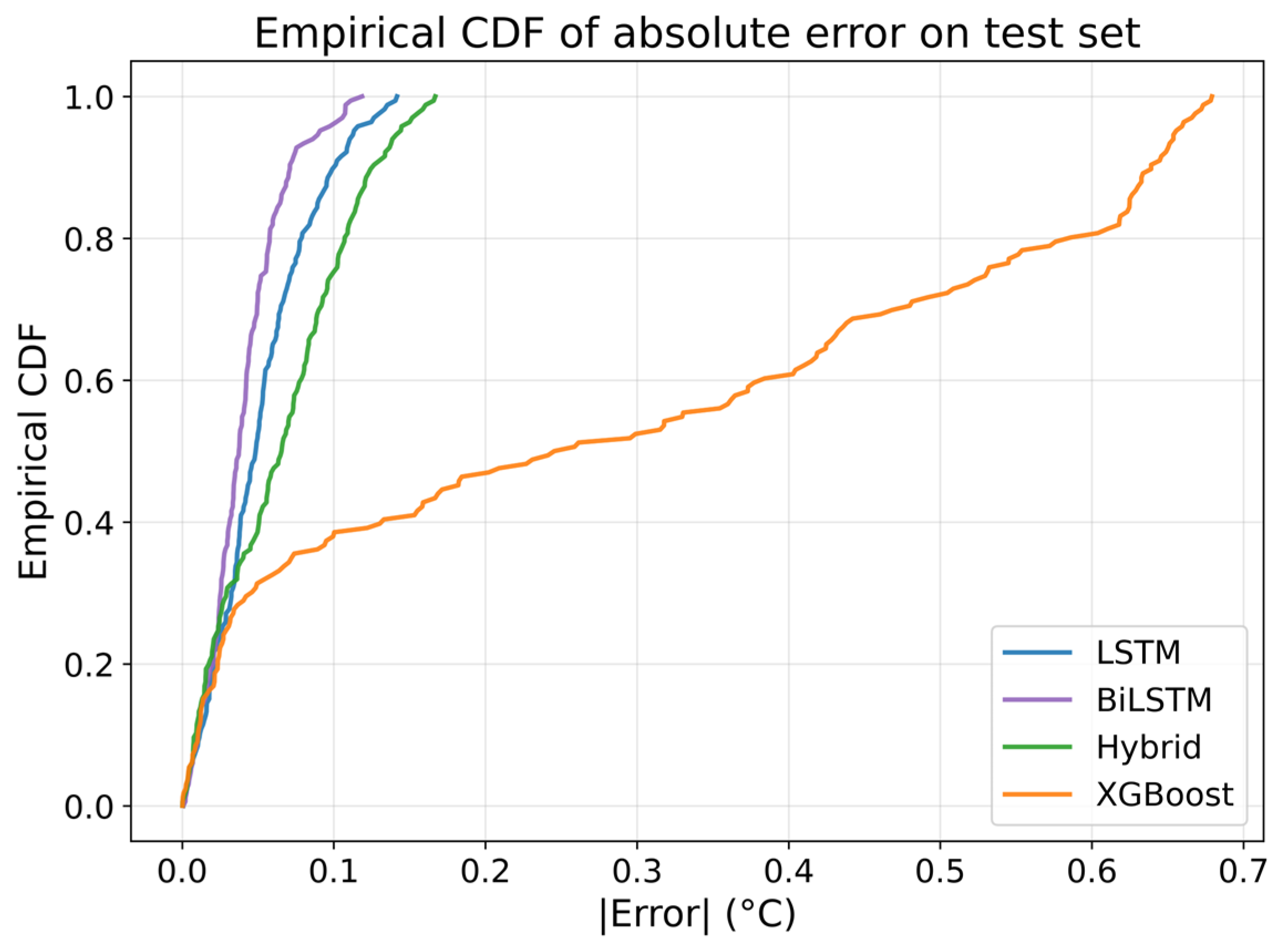
Reliability must also be quantified from a probabilistic standpoint, since thermal safety systems operate not on isolated error values, but on the likelihood that prediction deviations remain within acceptable bounds. The empirical cumulative distribution functions (ECDFs) in Figure 18, constructed using the indicator-based formulation in Equation (A84) and absolute error metric defined in Equation (A69), provide this statistical perspective by showing the fraction of predictions whose magnitude does not exceed a given error threshold.

The LSTM and BiLSTM curves rise steeply, with more than 90% of predictions confined to a narrow error range. This indicates that their recurrent dynamics, governed by Equations (A29)–(A39), yield not only low average error (Equation (A49)) but consistently low deviations across the entire test horizon. Such behavior demonstrates a high degree of predictable accuracy, meaning that the models do not occasionally produce large, unexpected errors that could compromise real-time control or mask incipient thermal instability.

The hybrid model exhibits a similar monotonic trend, albeit with slightly reduced steepness, reflecting the partial sensitivity introduced by the residual-learning mechanism in Equation (A73). In contrast, XGBoost progresses slowly along the CDF axis, with a long tail of large error values resulting from its inability to model cumulative thermal evolution through the additive ensemble structure in Equation (A27). This diffuse uncertainty profile confirms that tree-based learning lacks the thermodynamic continuity required for dependable temperature forecasting under dynamic electrochemical cycling.

These probabilistic results reinforce the central finding of this study: recurrent architectures do not merely produce accurate point estimates, they deliver statistically reliable predictions whose error behavior remains stable and bounded, satisfying core safety criteria for deployment in lithium-ion battery thermal monitoring and advanced battery-management systems.

An additional dimension of robustness is the model’s ability to sustain prediction fidelity as the operating temperature increases, where nonlinear electrochemical effects become more pronounced. Figure 19 plots prediction error against measured temperature, using the error definitions in Equations (A68) and (A77) and inverse scaling in Equations (A47) and (A48), to assess whether deviation magnitudes expand in high-temperature regimes associated with intensified heat generation described by Equations (A18)–(A20).

The LSTM and BiLSTM architectures maintain tightly bounded residuals across the full temperature range, indicating that their recurrent gating mechanisms, formalized in Equations (A29)–(A39), have internalized the coupling between temperature, current, and resistance evolution rather than treating temperature as an isolated time-series signal. This bounded behavior provides strong evidence that recurrent models learn the structure of electrothermal dynamics, enabling them to compensate for thermal nonlinearities that amplify at elevated operating states.

The hybrid model exhibits a gradual widening of error distribution, consistent with the residual-based correction mechanism in Equation (A73), yet it preserves predictable behavior without catastrophic divergence. XGBoost, however, deteriorates substantially with increasing temperature, producing error patterns that grow in magnitude and directionality. This degradation stems from the ensemble model’s inability to propagate thermal state information through the additive formulation in Equation (A27), leaving it insensitive to the nonlinear thermal transitions that dominate lithium-ion battery dynamics at higher temperatures.

These findings confirm that static regressors fail not because they lack accuracy at low temperatures, but because they cannot scale their predictive structure alongside electrothermal physics. Recurrent architectures, in contrast, exhibit temperature-invariant reliability, an indispensable property for real-time battery-management deployment where safe operation depends precisely on forecasting correctness under elevated and dynamically changing thermal conditions.

Collectively, the statistical evidence presented in Figure 12, Figure 13, Figure 14, Figure 15, Figure 16, Figure 17 and Figure 18 confirms that sequential deep learning architectures outperform conventional regressors not only in global accuracy, but across the full spectrum of reliability indicators, including temporal consistency, residual symmetry, probabilistic concentration, and temperature-dependent robustness. Their error signatures remain bounded, unbiased, and structurally coherent with the electrochemical temperature-generation mechanisms formalized in Equations (A18)–(A20), rather than exhibiting arbitrary statistical artifacts. These properties demonstrate that recurrent models do not merely fit temperature data, they internalize the physical processes governing it. Such thermodynamically consistent behavior is indispensable for real-world deployment, positioning these architectures as credible candidates for next-generation battery management systems where prediction trustworthiness is as critical as numerical precision.

3.8. Comparative Insight Against Conventional Machine Learning Models

The superiority of sequential learning architectures becomes increasingly apparent when contrasted with conventional machine learning regressors that lack temporal reasoning capabilities. While tree- and kernel-based models can approximate nonlinear static relationships, they are structurally incapable of encoding historical dependencies or anticipating future thermal transitions, both of which are intrinsic to lithium-ion battery temperature evolution. Battery temperature does not result from isolated measurements; it emerges from interacting electrochemical and thermal processes governed by load history, resistive losses, and entropy-driven effects. Models that treat temperature as an instantaneous value inevitably distort this physics, producing predictions that flatten, saturate, or drift away from the true thermal trajectory once operational conditions deviate from the patterns present during training.

These limitations manifest directly in error behavior: static regressors generate broad, skewed, and unstable residual distributions, revealing inference patterns that are reactive rather than thermodynamically informed. In contrast, sequential architectures such as LSTM and BiLSTM networks employ gated memory and recurrent state propagation to embed causal information about prior thermal states. This enables them to reconstruct the pathways through which heat accumulates, dissipates, and transitions, interpreting temperature not as an isolated numerical output, but as the emergent expression of an evolving electrothermal system. As a result, sequential models produce predictions that remain dynamically consistent with underlying thermophysical mechanisms, yielding error profiles that are structured, bounded, and physically interpretable.

3.9. Implications for Predictive Thermal Management in BMS

The findings of this study demonstrate that high-fidelity temperature prediction requires a modeling framework that perceives thermal evolution as a dynamic, physically governed process rather than a sequence of disconnected observations. Through the integration of thermal decomposition and recurrent deep learning, the proposed architecture elevates temperature estimation from passive measurement to predictive intelligence aligned with the strategic objectives of modern BMS.

Instead of responding to thermal events after they manifest, the system anticipates the trajectory of heat generation, identifies irreversible heating trends, and detects transitions indicative of electrochemical stress. This predictive capacity enables proactive intervention, optimizing cooling allocation, minimizing unnecessary derating, and reducing reliance on conservative safety margins. Moreover, the temporal stability and bounded error characteristics of the sequential models ensure persistent reliability across extended cycling, whereas conventional models typically degrade as aging alters internal resistance, heat capacity, and thermal response.

By producing coherent predictions across varying operating regimes, the proposed framework differentiates benign reversible fluctuations from hazardous irreversible heat buildup. This allows the BMS to make informed decisions regarding load scheduling, thermal actuation, and safety enforcement. Collectively, these capabilities transform the BMS from a reactive supervisory tool into an anticipatory thermal management platform that enhances battery lifespan, operational efficiency, and safety. The proposed modeling strategy therefore provides not only an accurate predictive mechanism, but a viable pathway toward self-adaptive thermal intelligence in next-generation electric mobility and stationary storage systems.

3.10. Numerical Performance Summary and Quantitative Assessment

The numerical results provide definitive evidence of the superiority of sequential deep learning models in reconstructing lithium-ion battery temperature evolution. Among all evaluated architectures, the BiLSTM achieves the highest predictive accuracy, exhibiting the lowest RMSE of 0.0406 °C, the smallest MAE of 0.0331 °C, and the highest explanatory power (R² = 0.9875). These results confirm that bidirectional temporal inference enhances predictive fidelity without compromising numerical stability.

The LSTM model follows closely, with RMSE = 0.0746 °C, MAE = 0.0666 °C, and R² = 0.9577, demonstrating strong ability to capture thermal propagation dynamics despite its unidirectional nature. The Hybrid LSTM-XGBoost configuration improves upon pure XGBoost but remains inferior to both recurrent models, achieving RMSE = 0.0707 °C and MAE = 0.0600 °C. This underscores the inherent limitation of residual boosting: temporal correlations cannot be reconstructed when they are absent from the core model representation.

In stark contrast, XGBoost yields an RMSE of 0.3794 °C and a negative R² (−0.0966), indicating performance worse than a naïve mean estimator. Its inability to model cumulative heating behavior results in saturation effects, distorted gradients, and broad, unbounded residuals under dynamic cycling conditions.

These metrics establish that sequential architectures do more than minimize numerical error, they faithfully reconstruct the physical trajectory of temperature evolution with statistically verifiable precision. Their low variance, bounded residual envelopes, and high explanatory power provide compelling justification for their deployment in safety-critical, real-time thermal monitoring and predictive BMS environments.

4. Conclusions

This study presented a unified, physics-informed, and data-driven framework for lithium-ion battery temperature prediction that integrates temperature decomposition, electrothermal heat generation modeling, and advanced sequential neural architectures. Unlike conventional regression approaches that treat temperature as an instantaneous numerical output, the proposed methodology interprets it as the coupled result of reversible and irreversible thermal processes. By embedding these thermodynamic principles directly into the learning pipeline, the framework transforms temperature prediction from correlation-based estimation into a physically grounded inferential process that reflects real battery behavior.

Extensive numerical experiments verified the decisive advantages of sequential architectures over classical machine learning techniques. The LSTM network achieved an RMSE of 0.0746 °C and an MAE of 0.0666 °C, which represents an 80% reduction in RMSE relative to XGBoost and a more than fourfold reduction in MAE. The Bidirectional LSTM further improved predictive fidelity, delivering the lowest errors (RMSE = 0.0406 °C, MAE = 0.0331 °C) and the highest explanatory power (R² = 0.9875). It also maintained more than 97% of predictions within plus or minus 0.1 °C, whereas classical regressors achieved less than 40% within the same range. These findings confirm that accurate temperature forecasting requires temporal learning and full electrothermal context rather than static or memoryless modeling strategies.

The practical relevance of the framework was demonstrated through the use of experimentally measured module temperatures that contain real sensor noise, current-driven fluctuations, and thermal lag. The decomposition and learning stages therefore operate on signals that reflect true operational conditions rather than synthetic or simulated data. This ensures that the resulting surrogate model can be transferred directly to battery modules and packs without architectural modification.

Because the predictions capture the reversible and irreversible heat processes that govern temperature rise, the model can be embedded into a battery management system to anticipate upcoming thermal excursions, support proactive thermal actuation, and maintain safe operating limits under variable duty cycles. The framework is also suitable for real-time deployment because the decomposition, normalization, and sequence generation steps require limited computational overhead. The strong generalization across operating regimes indicates that the approach can be extended to different chemistries and form factors with minimal retraining.

In summary, the integration of thermal decomposition with sequential deep learning represents a significant advance in lithium-ion battery temperature forecasting. It elevates temperature prediction from a retrospective measurement task to a forward-looking intelligence layer that delivers high accuracy, low uncertainty, and direct physical interpretability. Future work will extend the methodology to pack-level thermal propagation, incorporate current and voltage features for multi-input forecasting, and validate the framework under drive cycle conditions and accelerated stress testing. These directions will support the development of next generation, self-aware, and safety-critical battery management systems that require predictive rather than reactive thermal control.

References

1. Tarascon, J.-M.; Armand, M. Issues and challenges facing rechargeable lithium batteries. Nature 2001, 414, 359–367. [Google Scholar] [CrossRef]
2. Madani, S.S.; Shabeer, Y.; Allard, F.; Fowler, M.; Ziebert, C.; Wang, Z.; Panchal, S.; Chaoui, H.; Mekhilef, S.; Dou, S.X.; et al. A Comprehensive Review on Lithium-Ion Battery Lifetime Prediction and Aging Mechanism Analysis. Batteries 2025, 11, 127. [Google Scholar] [CrossRef]
3. Kabir, M.M.; Demirocak, D.E. Degradation mechanisms in Li-ion batteries: A state-of-the-art review. Int. J. Energy Res. 2017, 41, 1963–1986. [Google Scholar] [CrossRef]
4. Shabeer, Y.; Madani, S.S.; Panchal, S.; Mousavi, M.; Fowler, M. Different Metal–Air Batteries as Range Extenders for the Electric Vehicle Market: A Comparative Study. Batteries 2025, 11, 35. [Google Scholar] [CrossRef]
5. Feng, X.; Ouyang, M.; Liu, X.; Lu, L.; Xia, Y.; He, X. Thermal runaway mechanism of lithium ion battery for electric vehicles: A review. Energy Storage Mater. 2018, 10, 246–267. [Google Scholar] [CrossRef]
6. Mevawalla, A.; Shabeer, Y.; Tran, M.K.; Panchal, S.; Fowler, M.; Fraser, R. Thermal Modelling Utilizing Multiple Experimentally Measurable Parameters. Batteries 2022, 8, 147. [Google Scholar] [CrossRef]
7. Madani, S.S.; Shabeer, Y.; Nair, A.S.; Fowler, M.; Panchal, S.; Ziebert, C.; Chaoui, H.; Dou, S.X.; See, K.; Mekhilef, S.; et al. Advances in Battery Modeling and Management Systems: A Comprehensive Review of Techniques, Challenges, and Future Perspectives. Batteries 2025, 11, 426. [Google Scholar] [CrossRef]
8. Madani, S.S.; Allard, F.; Shabeer, Y.; Fowler, M.; Panchal, S.; Ziebert, C.; Mekhilef, S.; Dou, S.X.; See, K.; Wang, Z. Exploring the Aging Dynamics of Lithium-Ion Batteries for Enhanced Lifespan Understanding. J. Phys. Conf. Ser. 2025, 2968, 012017. [Google Scholar] [CrossRef]
9. Xing, Y.; Ma, E.W.M.; Tsui, K.L.; Pecht, M. Battery Management Systems in Electric and Hybrid Vehicles. Energies 2011, 4, 1840–1857. [Google Scholar] [CrossRef]
10. Madani, S.S.; Shabeer, Y.; Fowler, M.; Panchal, S.; Chaoui, H.; Mekhilef, S.; Dou, S.X.; See, K. Artificial Intelligence and Digital Twin Technologies for Intelligent Lithium-Ion Battery Management Systems: A Comprehensive Review of State Estimation, Lifecycle Optimization, and Cloud-Edge Integration. Batteries 2025, 11, 298. [Google Scholar] [CrossRef]
11. Xiao, Z.; Liu, C.; Zhao, T.; Kuang, Y.; Yin, B.; Yuan, R.; Song, L. Review—Online Monitoring of Internal Temperature in Lithium-Ion Batteries. J. Electrochem. Soc. 2023, 170, 057517. [Google Scholar] [CrossRef]
12. Jiang, J.; Ruan, H.; Sun, B.; Zhang, W.; Gao, W.; Wang, L.Y.; Zhang, L. A reduced low-temperature electro-thermal coupled model for lithium-ion batteries. Appl. Energy 2016, 177, 804–816. [Google Scholar] [CrossRef]
13. Harippriya, S.; Vigneswaran, E.E.; Jayanthy, S. Battery Management System to Estimate Battery Aging using Deep Learning and Machine Learning Algorithms. J. Phys. Conf. Ser. 2022, 2325, 012004. [Google Scholar] [CrossRef]
14. Shi, J.; Rivera, A.; Wu, D. Battery health management using physics-informed machine learning: Online degradation modeling and remaining useful life prediction. Mech. Syst. Signal Process. 2022, 179, 109347. [Google Scholar] [CrossRef]
15. Tian, Y.; Wen, J.; Yang, Y.; Shi, Y.; Zeng, J. State-of-Health Prediction of Lithium-Ion Batteries Based on CNN-BiLSTM-AM. Batteries 2022, 8, 155. [Google Scholar] [CrossRef]
16. Jiang, Y.; Yu, Y.; Huang, J.; Cai, W.; Marco, J. Li-ion battery temperature estimation based on recurrent neural networks. Sci. China Technol. Sci. 2021, 64, 1335–1344. [Google Scholar] [CrossRef]
17. Mallick, S.; Ahamed, F.; Ghosh, S.; Roy, T. KAN-Therm: A Lightweight Battery Thermal Model Using Kolmogorov-Arnold Network. arXiv 2025, arXiv:2509.09145. [Google Scholar]
18. Da Silva, C.M.; Akula, R.; Amon, C.H. Challenges and Opportunities in Hierarchical Multi-Length-Scale Thermal Modeling of Electric Vehicle Battery Systems. J. Heat Transf. 2025, 147, 124701. [Google Scholar] [CrossRef]
19. Zhao, Z.; Wang, Y.; Zhang, W.; Ba, Z.; Sun, L. Physics-informed neural networks in heat transfer-dominated multiphysics systems: A comprehensive review. Eng. Appl. Artif. Intell. 2025, 157, 111098. [Google Scholar] [CrossRef]
20. Carey, V. Machine Learning Enhancement of Heat Transfer Research and Technology Development. Annu. Rev. Heat Transf. 2025. [Google Scholar] [CrossRef]
21. Alawi, A.; Saeed, A.; Sharqawy, M.H.; Al Janaideh, M. A Comprehensive Review of Thermal Management Challenges and Safety Considerations in Lithium-Ion Batteries for Electric Vehicles. Batteries 2025, 11, 275. [Google Scholar] [CrossRef]
22. Zhang, X.; Xiang, H.; Xiong, X.; Wang, Y.; Chen, Z. Benchmarking core temperature forecasting for lithium-ion battery using typical recurrent neural networks. Appl. Therm. Eng. 2024, 248, 123257. [Google Scholar] [CrossRef]
23. Ren, F.; Cui, N.; Lu, D.; Li, C. Temperature prediction of lithium-ion battery based on adaptive GRU transfer learning framework considering thermal effects decomposition characteristics. Energy 2025, 322, 135504. [Google Scholar] [CrossRef]
24. Shen, K.; Xu, W.; Lai, X.; Li, D.; Meng, X.; Zheng, Y.; Feng, X. Physics-informed machine learning estimation of the temperature of large-format lithium-ion batteries under various operating conditions. Appl. Therm. Eng. 2025, 269, 126200. [Google Scholar] [CrossRef]
25. Cho, G.; Zhu, D.; Campbell, J.J.; Wang, M. An LSTM-PINN Hybrid Method to Estimate Lithium-Ion Battery Pack Temperature. IEEE Access 2022, 10, 100594–100604. [Google Scholar] [CrossRef]
26. Bamati, S.; Chaoui, H.; Gualous, H. Enhancing Battery Thermal Management With Virtual Temperature Sensor Using Hybrid CNN-LSTM. IEEE Trans. Transp. Electrif. 2024, 10, 10272–10287. [Google Scholar] [CrossRef]
27. Zafar, M.H.; Bukhari, S.M.S.; Houran, M.A.; Mansoor, M.; Khan, N.M.; Sanfilippo, F. DeepTimeNet: A novel architecture for precise surface temperature estimation of lithium-ion batteries across diverse ambient conditions. Case Stud. Therm. Eng. 2024, 61, 105002. [Google Scholar] [CrossRef]
28. Wang, Y.; Xiong, C.; Wang, Y.; Xu, P.; Ju, C.; Shi, J.; Yang, G.; Chu, J. Temperature state prediction for lithium-ion batteries based on improved physics informed neural networks. J. Energy Storage 2023, 73, 108863. [Google Scholar] [CrossRef]
29. Surya, S.; Samanta, A.; Marcis, V.; Williamson, S. Hybrid Electrical Circuit Model and Deep Learning-Based Core Temperature Estimation of Lithium-Ion Battery Cell. IEEE Trans. Transp. Electrif. 2022, 8, 3816–3824. [Google Scholar] [CrossRef]
30. Wei, Z.; Li, P.; Cao, W.; Chen, H.; Wang, W.; Yu, Y.; He, H. Machine learning-based hybrid thermal modeling and diagnostic for lithium-ion battery enabled by embedded sensing. Appl. Therm. Eng. 2022, 216, 119059. [Google Scholar] [CrossRef]
31. Lin, X.; Li, P.; Shao, L.; Shui, M.; Wang, D.; Long, N.; Ren, Y.; Shu, J. Lithium barium titanate: A stable lithium storage material for lithium-ion batteries. J. Power Sources 2015, 278, 546–554. [Google Scholar] [CrossRef]
32. Pang, H.; Wu, L.; Liu, J.; Liu, X.; Liu, K. Physics-informed neural network approach for heat generation rate estimation of lithium-ion battery under various driving conditions. J. Energy Chem. 2022, 78, 1–12. [Google Scholar] [CrossRef]
33. Zheng, Y.; Che, Y.; Hu, X.; Sui, X.; Teodorescu, R. Sensorless Temperature Monitoring of Lithium-Ion Batteries by Integrating Physics With Machine Learning. IEEE Trans. Transp. Electrif. 2023, 10, 2643–2652. [Google Scholar] [CrossRef]
34. Liu, Z.; Xiong, C.; Du, X. Study on Real-Time Battery Temperature Prediction Based on Coupling of Multiphysics Fields and Temporal Networks. IEEE Access 2024, 12, 105511–105526. [Google Scholar] [CrossRef]
35. Wang, B.; Chen, Z.; Zhang, P.; Deng, Y.; Li, B. The Lithium-Ion Battery Temperature Field Prediction Model Based on CNN-Bi-LSTM-AM. Sustainability 2025, 17, 2125. [Google Scholar] [CrossRef]
36. Teng, J.; Sun, X.; Wei, Z.; Li, Y.; Liu, B.; Liu, C.; Lu, H. A physics-guided method for predicting the core temperature of lithium-ion batteries. Energy 2025, 337, 138649. [Google Scholar] [CrossRef]
37. Al Tahhan, A.; Ramadan, M.; Choi, D.S.; Ahmed, R.; Ghazal, M.; AlKhedher, M. Recent advancements in Artificial Neural Network-based temperature prediction and management of lithium-ion batteries: A comprehensive review. AI Therm. Fluids 2025, 4, 100014. [Google Scholar] [CrossRef]
38. Jablonka, K.M.; Schwaller, P.; Ortega-Guerrero, A.; Smit, B. Leveraging large language models for predictive chemistry. Nat. Mach. Intell. 2024, 6, 161–169. [Google Scholar] [CrossRef]
39. Velumani, D.; Bansal, A. Thermal Behavior of Lithium- and Sodium-Ion Batteries: A Review on Heat Generation, Battery Degradation, Thermal Runway—Perspective and Future Directions. Energy Fuels 2022, 36, 14000–14029. [Google Scholar] [CrossRef]
40. Zhu, S.; He, C.; Zhao, N.; Sha, J. Data-driven analysis on thermal effects and temperature changes of lithium-ion battery. J. Power Sources 2021, 482, 228983. [Google Scholar] [CrossRef]
41. Shelly, T.J.; Weibel, J.A.; Ziviani, D.; Groll, E.A. Comparative analysis of battery electric vehicle thermal management systems under long-range drive cycles. Appl. Therm. Eng. 2021, 198, 117506. [Google Scholar] [CrossRef]
42. Amini, A.; Özdemir, T.; Ekici, Ö.; Başlamışlı, S.Ç.; Köksal, M. A thermal model for Li-ion batteries operating under dynamic conditions. Appl. Therm. Eng. 2021, 185, 116338. [Google Scholar] [CrossRef]
43. Dorogush, A.V.; Ershov, V.; Yandex, A.G. CatBoost: Gradient Boosting with Categorical Features Support. arXiv 2018, arXiv:1810.11363. [Google Scholar] [CrossRef]
44. Severson, K.A.; Attia, P.M.; Jin, N.; Perkins, N.; Jiang, B.; Yang, Z.; Chen, M.H.; Aykol, M.; Herring, P.K.; Fraggedakis, D.; et al. Data-driven prediction of battery cycle life before capacity degradation. Nat. Energy 2019, 4, 383–391. [Google Scholar] [CrossRef]
Figure 1. Schematic overview of abuse-induced failure pathways in LIBs, illustrating the sequence from thermal perturbation to hazardous runaway outcomes.
Wevj 17 00002 g001
Figure 2. Conceptual workflow of BMS-integrated data acquisition, preprocessing, predictive temperature estimation, and thermal decision-making logic.
Wevj 17 00002 g002
Figure 3. Temperature-dependent operational envelope of LIBs, showing reduced power capability at low temperatures, increased degradation at elevated temperatures, and the narrow optimal band where safe, efficient operation is maintained.
Wevj 17 00002 g003
Figure 4. Conceptual diagram of the proposed thermal decomposition and prediction framework.
Wevj 17 00002 g004
Figure 5. Workflow of the decomposition-enabled temperature prediction pipeline.
Wevj 17 00002 g005
Figure 6. Seasonal temperature (T_Seasonal) component alongside the charge–discharge current profile.
Wevj 17 00002 g006
Figure 7. Decomposed temperature signal components and corresponding heat-generation profiles.
Wevj 17 00002 g007
Figure 8. Preprocessing workflow applied to the measured module temperature showing (a) raw versus cleaned thermal data, (b) normalized temperature profile z(t), and (c) temporally ordered train-validation-test split used to ensure causally consistent model development.
Wevj 17 00002 g008
Figure 9. Training and validation loss curves for the LSTM and BiLSTM architectures showing rapid convergence to low error and closely aligned trajectories, indicating stable learning of thermal dynamics without overfitting.
Wevj 17 00002 g009
Figure 10. Measured versus predicted module temperatures across the full test horizon for LSTM, BiLSTM, hybrid, and XGBoost models, showing the superior tracking fidelity of recurrent architectures under dynamic cycling conditions.
Wevj 17 00002 g010
Figure 11. Zoomed-in comparison of temperature predictions over the most challenging test interval, demonstrating the BiLSTM model’s superior responsiveness to rapid electrothermal transitions.
Wevj 17 00002 g011
Figure 12. Time-resolved residual temperature errors for the LSTM, BiLSTM, and hybrid models, illustrating bounded and unbiased prediction behavior without drift.
Wevj 17 00002 g012
Figure 13. Rolling RMSE analysis across the test sequence, confirming the superior localized robustness of recurrent architectures under evolving thermal stress.
Wevj 17 00002 g013
Figure 14. RMSE comparison of LSTM, BiLSTM, hybrid, and XGBoost temperature prediction models over the full test horizon, illustrating the dominance of recurrent architectures in minimizing global prediction error.
Wevj 17 00002 g014
Figure 15. Residual error distributions for each model, revealing compact, symmetric structures for recurrent architectures and dispersed, skewed profiles for tree-based regression.
Wevj 17 00002 g015
Figure 16. Scatter comparison between measured and predicted temperatures, with the ideal 45° line indicating proportional accuracy and confirming the superior structural fidelity of recurrent architectures.
Wevj 17 00002 g016
Figure 17. Absolute error boxplots demonstrating the narrow, stable error bounds of LSTM and BiLSTM models compared to the highly variable distributions produced by XGBoost.
Wevj 17 00002 g017
Figure 18. Empirical cumulative distribution functions of absolute prediction error, showing that recurrent models achieve more than 90% of predictions within a tight error threshold, while XGBoost exhibits diffuse uncertainty.
Wevj 17 00002 g018
Figure 19. Prediction error as a function of operating temperature, confirming that recurrent architectures maintain bounded, physically consistent behavior even at elevated thermal states.
Wevj 17 00002 g019
Disclaimer/Publisher’s Note: The statements, opinions and data contained in all publications are solely those of the individual author(s) and contributor(s) and not of MDPI and/or the editor(s). MDPI and/or the editor(s) disclaim responsibility for any injury to people or property resulting from any ideas, methods, instructions or products referred to in the content.