Fusing Direct and Indirect Visual Odometry for SLAM: An ICM-Based Framework

Abstract

The loss of localization in robots navigating GNSS-denied environments poses a critical challenge that can compromise mission success and safe operation. This article presents a method that fuses visual odometry outputs from both direct and feature-based (indirect) methods using Iterated Conditional Modes (ICMs), an efficient iterative optimization algorithm that maximizes the posterior probability in Markov random fields, combined with uncertainty-aware gain adjustment to perform pose estimation and mapping. The proposed method enhances the performance of visual localization and mapping algorithms in low-texture or visually degraded scenarios. The method was validated using the TUM RGB-D benchmark dataset and through real-world tests in both indoor and outdoor environments. Outdoor experiments were conducted on an electric vehicle, where the method maintained stable tracking. These initial results suggest that the technique could be transferable to electric vehicle platforms and applicable in a variety of real-world conditions.

1. Introduction

Simultaneous localization and mapping enables robotic systems to concurrently construct a representation of their environment and determine their own position within that representation [1]. For mobile robots, whether they move autonomously or with the assistance of an operator, the integration of SLAM systems in GNSS-denied environments is imperative [2]. Typically, these systems rely on the fusion of data from diverse sensor suites, such as monocular and stereoscopic vision systems, LiDAR, and inertial sensors [3,4].

With the rise of electric vehicles (EVs), visual-based localization has gained attention as a cost-effective alternative to LiDAR-centric systems. A recent review highlights the growing interest in multi-sensor fusion SLAM approaches for intelligent EV navigation [5]. Moreover, recent studies on visual perception systems in electric vehicles emphasize the importance of robust feature tracking and illumination-invariant algorithms to ensure localization reliability under dynamic and visually degraded conditions [6].

When cameras are the only sensor in the system, visual SLAM (V-SLAM) is performed. V-SLAM techniques are based on visual odometry (VO), which can be defined as the method for estimating an agent’s egomotion (human, robot, vehicle, etc.) based only on the input of a single or several cameras [7,8,9]. Within this domain, two primary image processing paradigms can be distinguished: direct methodologies, which use pixel brightness and position for motion estimation, and feature-based methodologies, which construct a scene representation prior to motion estimation.

Direct methods select a subset of pixels through a pixel selection strategy and apply a direct image alignment process to estimate camera motion. The influential contributions of Engel et al. [10,11,12] are pivotal for understanding the direct visual odometry. In  [12], the authors proposed estimating camera motion by performing the minimization of a photometric error function derived from the observed pixel intensities. Engel’s ideas inspired a significant amount of recent literature [13,14,15,16].

Feature-based visual odometry pipeline, on the other hand, starts by extracting a set of features from the input frame, followed by a feature matching procedure with the previous frame. The resulting correspondences are then used to estimate camera motion. The cornerstone of current feature-based methods [17,18,19,20,21] is ORB-SLAM [22]. This system performs the aforementioned steps based on the extraction and matching of a set of ORB descriptors from the input frame. After an initial guess of the agent’s pose is obtained, this system refines the pose by a process named motion-only Bundle Adjustment.

While both approaches have proven effective, each comes with its limitations. Direct methods assume photometric consistency (i.e., pixel intensities remain constant across frames), a condition that can be easily violated by lighting changes, leading to errors in the motion estimation. Feature-based methods, on the other hand, suffer in low-texture environments where feature extraction and matching become unreliable, often resulting in tracking loss. Despite these limitations, the two methods are complementary. In low gradient scenarios, direct methods can still recover a good pose estimate, while feature-based methods are resilient to brightness variations when reliable features are present.

This work proposes a modular fusion architecture that combines the outputs of direct and feature-based visual odometry within a single framework. By exploiting their complementary characteristics, the system mitigates the risk of full tracking loss and promotes more reliable pose estimation.

Since the beginning of the 21st century, the SLAM problem has been extensively studied using graph-based models. Folkesson and Christensen introduced the GraphSLAM system which finds the best robot trajectory using a nonlinear optimization technique [23]. Graph theory allows one to intuitively illustrate the states of a system with their interdependencies. In a SLAM context, nodes represent the robot’s poses at different time steps, and edges encode spatial constraints between these poses. These constraints arise from sensor observations or the robot’s motion. Once this graph is established, the map is obtained by estimating the spatial arrangement of the nodes that best aligns with the constraints defined by the edges [24].

Although graph-based methods offer a strong framework, full pose graph optimization heavily relies on a loop closure event. Without this crucial constraint, the optimization problem lacks sufficient information, leading to reduced global accuracy in the estimated map and trajectory [25].

Markov random fields (MRFs) can be used to solve the SLAM problem if the conditional probabilities of the model are consistent with the topological structure of the graph [26]. The potentiality of working in the MRF context has been reported in [27], where the authors proposed a fully Bayesian way to solve the simultaneous localization and spatial prediction (SLAP) problem by using a Gaussian Markov random field (GMRF) model with satisfactory results. In [28], GMRFs are integrated for modeling information distribution. The study presents a computationally efficient strategy for autonomous exploration in 3D environments.

In a previous study [29], Gimenez et al. proposed a general method for localization and mapping in the MRF context. This method employs the Iterated Conditional Modes (ICMs) algorithm, which systematically finds a configuration of states that locally maximizes the posterior probability, given a set of observations, within a Markovian model. The approach was evaluated using a differential drive mobile robot equipped with a laser range finder. The robot traversed different structured environments with a finite set of known landmarks. In a subsequent study [30], the mapping is based on a point cloud generated from successive environmental observations, with each location assigned an occupancy probability using 2D kernel density estimation (KDE). To manage point cloud growth and adapt to dynamic environments, the system incorporates a novel recursive subsampling method that also helps in gradually discarding moving objects. This approach facilitates online point probability calculations and bypasses the complex data association problem inherent in other map representations. In both use cases, the system successfully recovered the robot’s trajectory and produced accurate map estimates. In this paper, we present an enhanced version of the framework described in [29]. The proposed framework is designed to incorporate diverse observation models (regardless of the sensor type and data characteristics), odometry sources, and any map representation. Our contributions can be summarized as follows:

• We propose a novel, modular approach for the unified fusion of direct and feature-based odometry. This integration improves pose estimation reliability and reduces tracking failure, particularly in challenging conditions.
• Novel potential functions are introduced to enable 6-DoF pose estimation using ICM.
• Dynamically adjusted gain values are integrated into the ICM algorithm to enhance robustness against tracking loss in visually degraded or low-texture environments.

The remainder of the paper is organized as follows. Section 2 provides an overview of the system and the theoretical foundations of the ICM method, followed by a description of the proposed iterative fusion process and the adaptable gain value scheme. Section 3 presents the results obtained from both benchmark datasets and real-world experiments. The findings are discussed in Section 4, and the conclusions are drawn in Section 5.

2. Materials and Methods

2.1. System Overview

Figure 1 illustrates the modular structure of the proposed system. Input RGB-D frames are simultaneously processed by a feature-based VO module and a direct VO module, each producing an independent estimate of the agent’s pose. At each time step, the direct VO module also generates a set of 2000 observations, which are subsequently transformed into a point cloud. These observations are fed into a dedicated map handler that builds and maintains both a local map and a global map. The local map supports internal computations, while the global map provides a visual representation of the reconstructed environment.

The ICM module receives the odometry measurements, the local map, and the observations to yield a refined estimate of the camera’s pose $x_t$. Inside this module, each one of the inputs is represented as a potential function. As will be described in Section 2.4.1, it is through these potential functions that the fusion of measurements from direct and feature-based odometry is achieved.

The 6-DoF pose vector of the camera at each time is defined as ${\mathbf{x}}_{\mathbf{t}}=[x,y,z,\varphi ,\theta ,\psi ]$, with x, y and z being the translational part of the vector, and $\varphi$, $\theta$, and $\psi$ being the associated angles corresponding to rotations in the x, y and z axes, respectively. To enable a direct comparison with the ground truth data available in state-of-the-art datasets, the output pose of the proposed system is expressed in the Lie group $SE\left(3\right)$ as

$$\xi =\left[\begin{array}{cc}\mathrm{\Gamma }& \tau \\ \mathbf{0}& 1\end{array}\right]$$

(1)

where $\tau ={[x,y,z]}^T$ of the ${\mathbf{x}}_{\mathbf{t}}$ vector and the rotation matrix R, also denoted as $R\left(\varphi ,\theta ,\psi \right)$, is defined as the concatenation of the rotations around each coordinate axis

$$\mathrm{\Gamma }=\mathrm{\Gamma }\left(\varphi ,\theta ,\psi \right)={\mathrm{\Gamma }}_z\left(\psi \right){\mathrm{\Gamma }}_y\left(\theta \right){\mathrm{\Gamma }}_x\left(\varphi \right)$$

(2)

where

$${\mathrm{\Gamma }}_x\left(\varphi \right)=\left[\begin{array}{ccc}1& 0& 0\\ 0& cos\varphi & -sin\varphi \\ 0& sin\varphi & cos\varphi \end{array}\right],{\mathrm{\Gamma }}_y\left(\theta \right)=\left[\begin{array}{ccc}cos\theta & 0& sin\theta \\ 0& 1& 0\\ -sin\theta & 0& cos\theta \end{array}\right],{\mathrm{\Gamma }}_z\left(\psi \right)=\left[\begin{array}{ccc}cos\psi & -sin\psi & 0\\ sin\psi & cos\psi & 0\\ 0& 0& 1\end{array}\right]$$

The design of the odometry modules is inspired by state-of-the-art systems such as ORB-SLAM and DSO. Nevertheless, such systems require C++-based libraries to perform pose estimation and optimization, which posed compatibility challenges for this study’s Python 3.8-based framework. Therefore, a custom implementation was developed to maintain the full control over the pipeline and ensure portability.

2.2. Theoretical Background on Iterated Conditional Modes

Given a finite set of nodes $\mathcal{V}$ in a graph, a random field (RF) is an array of random variables $\mathbf{X}=\{X_v:vs.\in \mathcal{V}\}$. The subset of random variables corresponding to a node subset $A\subseteq \mathcal{V}$ is denoted as $X_A=\{X_a:a\in A\}$, while the set of all variables except $X_v$ is written as $X_{-v}=\{X_a:a\in \mathcal{V},a\ne vs.\}$. Two nodes are said to be neighbors if they are connected by an edge in the graph, and the set of all neighbors of a node v is denoted by $\partial v$. A clique $C\subseteq \mathcal{V}$ is a subset of nodes in which every pair of nodes is mutually connected. The set of all cliques in the graph is denoted by $\mathcal{C}$.

Let $\mathrm{\Omega }$ represent the set of all possible states of the random field $\mathbf{X}$, and let P be the probability defined over $\mathrm{\Omega }$ such that $P\left(\omega \right)$ denotes the probability of the RF $\mathbf{X}$, assuming the state $\omega$. The conditional probability that $X_v$ takes a value ${\omega }_v$ given that $X_A$ takes value ${\omega }_A$ is denoted by $P\left({\omega }_v\right|{\omega }_A)$. Then, a random field $\mathbf{X}$ defined over a graph with associated probability P is a Markov random field (MRF) if

$$P\left({\omega }_v\right|{\omega }_{-v})=P\left({\omega }_v\right|{\omega }_{\partial v})\forall vs.\in \mathcal{V}$$

(3)

That is, the probability of observing each ${\omega }_v$, given all other states, can be computed solely from the values in its neighborhood.

Now, consider a family of potentials $\{{\mathrm{\Phi }}_C:C\in \mathcal{C}\}$, where each ${\mathrm{\Phi }}_C$ is a function that assigns a real-valued confidence measure to each local configuration ${\omega }_C$, such that

$${\mathrm{\Phi }}_C\left({\omega }_C\right)>{\mathrm{\Phi }}_C\left({\omega }_C^{\prime }\right)$$

(4)

when configuration ${\omega }_C$ is more likely than ${\omega }_C^{\prime }$.

Then, assuming

$$P\left(\omega \right)\propto exp\left\{\sum _{C\in \mathcal{C}}{\mathrm{\Phi }}_C\left({\omega }_C\right)\right\}$$

(5)

then it can be shown that

$$P\left({\omega }_v\right|{\omega }_{\partial v})=P\left({\omega }_v\right|{\omega }_{-v})\propto exp\left\{\sum _{C\in \mathcal{C}:vs.\in C}{\mathrm{\Phi }}_C\left({\omega }_C\right)\right\}$$

(6)

Finding the global maximum of the joint probability defined in Equation (5) requires an appropriate optimization method. Simulated annealing (SA) is a well-known iterative approach capable of addressing this task. Although SA guarantees theoretical convergence to the global optimum, its application is often impractical due to its high computational cost. Given these conditions, the Iterated Conditional Modes (ICM) algorithm rises as a practical alternative. This method iteratively optimizes the conditional probabilities in Equation (6) at a lower computational cost. While ICM’s resulting configuration typically converges to the local maximum of the Equation (5) closest to the initial state, it can yield highly satisfactory results when the initialization is appropriately chosen [31].

2.3. Potential Functions Definition

In order to solve for the most likely configuration of the system at each timestep t, it is necessary to define potential functions $\mathrm{\Phi }$. Each $\mathrm{\Phi }$ must assign a real-valued confidence measure to each local configuration, and fulfill Equation (4).

The flexibility of this proposal lies in the fact that it is possible to define a $\mathrm{\Phi }$ function for each information source within the system, regardless of its nature. The most important design requirement is that these functions must penalize incorrect configurations while rewarding correct ones.

As seen in Equations (5) and (6), the objective function is expressed as the sum of all system potentials. This formulation allows an additional layer of flexibility, as each potential can include a gain factor K. As a result, Equation (5) becomes a weighted sum, where each term can reflect the relative confidence of the user in the corresponding sensor measurement.

Next, we describe the potential functions used for the experimental evaluation of this system. Subscripts on the pose vector indicate the time range considered for estimation; for instance, $x_{t-1:t+1}$ denotes that poses at time steps $t-1$, t, and $t+1$ are included in the calculation. Additional information and definitions referring to other types of sensors can be found in [30].

2.3.1. Odometry Potential

In this article, we define odometry ${\widehat{x}}_t$ as any estimation of the pose $x_t$ obtained from internal sensory inputs. Over time, such estimates are prone to substantial drift due to accumulated error. However, if the relative change between consecutive estimations is considered, then $x_t-x_{t-1}$ can be estimated with ${\widehat{x}}_t-{\widehat{x}}_{t-1}$. A possible way to express this relationship could be

$${\mathrm{\Phi }}_{\left\{x_{t-1:t}\right\}}^{\mathrm{odo}}\left(x_{t-1:t}\right)=-K_{\mathrm{odo}}\left|\right|s\left(x_{t-1:t}\right)-s\left({\widehat{x}}_{t-1:t}\right){\left|\right|}^2$$

(7)

where $s\left(x_{t-1:t}\right)$ is defined as

$$s\left(x_{t-1:t}\right)=R_c\left(x_{t-1;\varphi ,\theta ,\psi }\right)(x_{t;x,y,z}-x_{t-1;x,y,z})$$

(8)

and $R_c\left(x_{t-1;\varphi ,\theta ,\psi }\right)={\mathrm{\Gamma }}^T$ is a matrix designed to cancel the rotation of the odometry vector, with $\mathrm{\Gamma }$ defined in Equation (2).

2.3.2. Continuity Potential

To ensure smooth pose transitions over time, introducing a potential function that penalizes abrupt positional changes may be beneficial.

The expression in Equation (9) enforces the value of $x_t$ to remain close to those of its neighboring nodes in the graph.

$${\mathrm{\Phi }}_{\left\{x_{t-2:t}\right\}}^{\mathrm{cont}}\left(x_{t-2:t}\right)=-K_{\mathrm{cont}}\left|\right|s\left(x_{t-2:t-1}\right)-s\left(x_{t-1:t}\right){\left|\right|}^2$$

(9)

This potential function reduces the system’s sensitivity to inaccurate pose estimates caused by poor data association or outliers.

2.3.3. Mapping and Observations Potential

Let us consider the general case of an agent navigating through an unknown environment. Traditional landmark-based SLAM systems depend on the presence and constant re-observation of distinctive landmarks of the map. Without prior knowledge of their locations, these systems can become infeasible in practice, especially in unfamiliar or large-scale settings [32].

Now, suppose that the system is equipped with a sensor array capable of creating an abstraction of the environment (e.g., a point cloud). Additionally, assume it has sufficient memory to store observations acquired at neighboring nodes in the graph. Under these conditions, this memory can be interpreted as a local map $\mathbf{m}$. Each point in the point cloud is an observation of the environment.

At each time step t, the system captures a set of observations $z_t=\{z_{t,i}:i=1,\dots ,n_t\}$, where $n_t$ denotes the number of points observed at that moment. These observations establish a connection between the robot’s pose $x_t$ and $\mathbf{m}$. The local map $\mathbf{m}$ is constructed by aggregating observations from several time steps. As a result, the local map contains $N_l$ points, with $N_l>n_t$, since it combines information from multiple frames.

Once the nature of the observations and the map has been established, a potential function can be defined to quantify the correspondence between the set of observations and the map. If the $N_l$ points in the local map are treated as known position landmarks for the current time, then the corresponding observation potential can be defined as

$${\mathrm{\Phi }}_{\{x_t,\mathbf{m}\}}^{\mathrm{obs}}(x_t,\mathbf{m})=-K_{\mathrm{obs}}{\displaystyle \frac{1}{n_t}}\sum _{i=1}^{n_t}\arg \underset{l}{min}\left|\right|h(x_t,z_{t,i})-m_l{\left|\right|}^2$$

(10)

where $h(x_t,z_{t,i})$ represents the position of a given observation $z_{t,i}$ given $x_t$ and $m_l\in N_l$ is a point of the local map.

In this article, observations take the form of point clouds. Each element of the point cloud is represented as $z_{t,i}=[z_{t,i,x},z_{t,i,y},z_{t,i,z}]\in {\mathbb{R}}^3$. Given $x_t$, the position of $z_{t,i}$ is obtained by

$$h(x_t,z_{t,i})=\mathrm{\Gamma }\left(t\right)z_{t,i}+\tau \left(t\right)$$

(11)

with $\mathrm{\Gamma }\left(t\right)=\mathrm{\Gamma }(x_{t,\varphi },x_{t,\theta },x_{t,\psi })$ and $\tau \left(t\right)=[x_{t,x},x_{t,y},x_{t,z}]$

2.4. Data Fusion via ICM

In this section, the iterative process for the sensor fusion via an ICM implementation is described. First, a method to initialize the system states is proposed in Section 2.4.1. Next, the optimization process is described in Section 2.4.2.

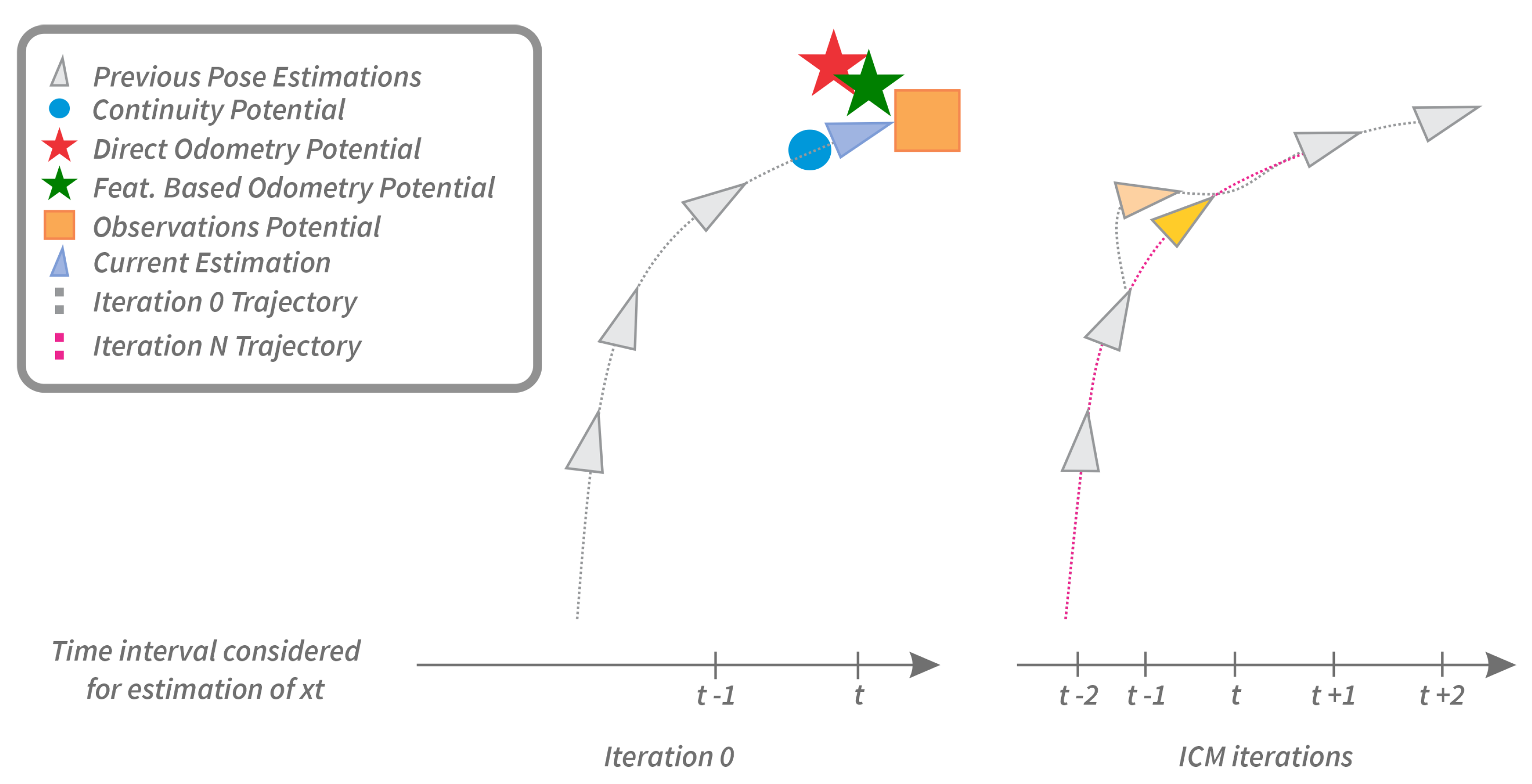
However, before delving into the mathematical concepts relevant to data fusion through ICM, these ideas are first graphically illustrated using the example shown in Figure 2. The system states are initialized in what is referred to as iteration 0 of the algorithm, displayed on the left-hand side of the figure. To identify the optimal configuration of the states (highlighted in the image with the light-blue triangle), the algorithm draws upon present and past information from the defined potentials. In this case, it integrates information from direct and feature-based odometry, the continuity potential, and the observation potential. For the clarity of presentation, only the measurements from the current time step of each potential are depicted in the image.

After the exploration concludes, the system halts, or a loop closure occurs, and the ICM algorithm transitions into a second phase, referred to as ICM iterations (right side of Figure 2). Unlike iteration 0, where future information is unknown, iterations N refine the trajectory using the complete set of past, present, and future data from the potential functions. In this way, the pose at a given time (e.g., marked in transparent orange) is optimized into a refined estimate (yellow), improving upon the initial iteration.

2.4.1. Initialization

As stated in Section 2.2, the ICM algorithm converges to a high-quality local maximum if the initial states are appropriately chosen. Thus, the success of the method relies heavily on the quality of the initialization phase (iteration 0 of ICM). This phase proceeds until the system stops, exploration ceases, or a loop closure is detected. Let $T_f$ represent the time at which iteration 0 terminates under any of these conditions.

During the exploration of an unknown environment, the robot only has access to current and past data. We propose an online initialization strategy that leverages this information to obtain an initial estimate of the robot’s trajectory ${\mathbf{x}}^{\left(0\right)}$ and the local map ${\mathbf{m}}^{\left(0\right)}$. Algorithm 1 describes how to compute the pose $x_t^{\left(0\right)}$ given the available data.

Algorithm 1 Online ICM initialization.

Ensure: $x_0^{\left(0\right)},{\mathbf{m}}^{\left(0\right)}$    while $t<T_f$ do $$\begin{array}{c}\hfill \begin{array}{c}\hfill x_t^{\left(0\right)}=\arg \underset{\mathbf{x}}{min}\{-K_{\mathrm{odo}}\left|\right|s\left(x_{t-1:t}\right)-s\left({\widehat{x}}_{t-1:t}\right){\left|\right|}^2-\\ \hfill K_{\mathrm{cont}}\left|\right|s\left(x_{t-2:t-1}\right)-s\left(x_{t-1:t}\right){\left|\right|}^2-\\ \hfill -K_{\mathrm{obs}}{\displaystyle \frac{1}{n_t}}\sum _{i=1}^{n_t}\arg \underset{l}{min}\left|\right|h(x_t,z_{t,i})-m_l{\left|\right|}^2\}\end{array}\end{array}$$ (12)    Update local map ${\mathbf{m}}^{\left(0\right)}$ given the estimated $x_t^{\left(0\right)}$ and evaluate candidate points for the global map end while

In this implementation, the integration of both odometry sources leads to the following extended form of Equation (12):

$$\begin{array}{c}\hfill x_t^{\left(0\right)}=\arg \underset{\mathbf{x}}{min}\{K_{\mathrm{odo}}^{dir}\left|\right|s\left(x_{t-1:t}\right)-s\left({\widehat{x}}_{t-1:t}^{dir}\right){\left|\right|}^2+K_{\mathrm{odo}}^{feat}\left|\right|s\left(x_{t-1:t}\right)-s\left({\widehat{x}}_{t-1:t}^{feat}\right){\left|\right|}^2+\\ \hfill K_{\mathrm{cont}}\left|\right|s\left(x_{t-2:t-1}\right)-s\left(x_{t-1:t}\right){\left|\right|}^2+K_{\mathrm{obs}}{\displaystyle \frac{1}{n_t}}\sum _{i=1}^{n_t}\arg \underset{l}{min}\left|\right|h(x_t,z_{t,i})-m_l{\left|\right|}^2\}\end{array}$$

(13)

In this way, Equation (13) enables the fusion of the outputs from the odometry systems with each other and with the continuity and observation potentials, so that, during optimization, state configurations inconsistent with the pose graph are penalized while correct configurations are rewarded.

2.4.2. ICM Iterations

Once the system states have been initialized, an optimization procedure is performed using N ICM iterations. This process leverages information from the state currently being updated as well as from past and future data. As a result, Equations (7) and (9) can be modified to account for the future data as follows:

$${\mathrm{\Phi }}_{\left\{x_{t-1:t+1}\right\}}^{\mathrm{odo}}\left(x_{t-1:t}\right)=-K_{\mathrm{odo}}\left[{\mathrm{\Phi }}_{\left\{x_{t-1:t}\right\}}^{\mathrm{odo}}\left(x_{t-1:t}\right)+{\mathrm{\Phi }}_{\left\{x_{t:t+1}\right\}}^{\mathrm{odo}}\left(x_{t:t+1}\right)\right]$$

(14)

$${\mathrm{\Phi }}_{\left\{x_{t-2:t+2}\right\}}^{\mathrm{cont}}\left(x_{t-2:t}\right)=-K_{\mathrm{cont}}\left[{\mathrm{\Phi }}_{\left\{x_{t-2:t}\right\}}^{\mathrm{cont}}\left(x_{t-2:t}\right)+{\mathrm{\Phi }}_{\left\{x_{t-1:t+1}\right\}}^{\mathrm{cont}}\left(x_{t-1:t+1}\right)+{\mathrm{\Phi }}_{\left\{x_{t:t+2}\right\}}^{\mathrm{cont}}\left(x_{t:t+2}\right)\right]$$

(15)

During the optimization process detailed in Algorithm 2, a sweep over the states obtained in the initialization is performed. These states are arbitrarily sorted according to a visit scheme (e.g., $x_0$, $x_1$,..., $x_{T_f}$). In this step, each node is visited according to the visit scheme, jointly optimizing (10), (14), and (15) to find the most suitable configuration of the system. This process is repeated during N ICM iterations.

Algorithm 2 ICM iterations.

Ensure: ${\mathbf{x}}^{\left(0\right)},{\mathbf{m}}^{\left(0\right)}$, and a number of ICM iterations to perform N.    Generate a visit scheme, i.e., choose in what order the model states ($x_1,x_2...,x_{T_F}$) will be updated.         for n < N do           for each $x_t$ in the visit scheme do $$\begin{array}{c}\hfill x_t^{\left(n\right)}=\arg \underset{\mathbf{x}}{min}\{-K_{\mathrm{odo}}\left[\left|\right|s\left(x_{t-1:t}^{\left(n\right)}\right)-s\left({\widehat{x}}_{t-1:t}\right){\left|\right|}^2+\left|\right|s(x_{t:t+1)}^{(n-1)}-s\left({\widehat{x}}_{t:t+1}\right){\left|\right|}^2\right]+\\ \hfill -K_{\mathrm{cont}}[\left|\right|s\left(x_{t-2:t-1^{\left(n\right)}}^{\left(n\right)}\right)-s\left(x_{t-1:t}^{\left(n\right)}\right){\left|\right|}^2+\left|\right|s\left(x_{t-1:t}^{\left(n\right)}\right)-s\left(x_{t:t+1}^{(n-1)}\right){\left|\right|}^2+\\ \hfill \left|\right|s\left(x_{t:t+1}\right)-s\left(x_{t+1:t+2}^{(n-1)}\right){\left|\right|}^2]+\\ \hfill -K_{\mathrm{obs}}{\displaystyle \frac{1}{n_t}}\sum _{i=1}^{n_t}\arg \underset{l}{min}\left|\right|h(x_t,z_{t,i})-m_l^{\left(n\right)}{\left|\right|}^2\}\end{array}$$     end for end for         Update global map given the optimized trajectory.

Note that the mathematical expression for the observations’ potential does not change. However, given that posterior information is available, the local map used in this function will be built in each iteration with observations from $x_{t-2}$, $x_{t-1}$, $x_t$, $x_{t+1}$, and $x_{t+2}$. The number N of ICM iterations can be as large as needed, and depends on the quality of the initialization. Additionally, a termination criterion can be added to stop iterating.

2.5. Adaptable Gain Values

To significantly reduce the likelihood of tracking failure, the system needs to dynamically adapt to varying visual conditions. One way to achieve this is to change the effect of the odometry measurements in the final result.

In [10], the authors considered the inverse of the Hessian from the last iteration in the pose estimation algorithm as an estimate of the covariance of the estimation. Under this assumption, we propose to extract an uncertainty measure for the pose estimation provided by the visual odometry modules by

$${\sigma }_{\xi }={\left(\prod _{i=1}^n\sqrt{v_i}\right)}^{1/n}$$

(16)

where $\xi$ refers to the pose representation (1), and $v_i$ represents the diagonal elements of the Hessian inverse matrix. We consider that the aforementioned Hessian matrix is available to the system.

Odometry gains are expected to behave inversely with respect to the measurement uncertainty (16). Higher uncertainty should yield lower gains, while reliable measurements should result in higher gains. To model this relationship, a gain adjustment function is defined as

$$K_{\mathrm{odo}}=e^{\alpha ·{\left({\sigma }_{\xi }\right)}^{\beta }}$$

(17)

The parameters $\alpha$ and $\beta$ determine how pose uncertainty affects the weighting factor. Specifically, $\alpha$ regulates the sensitivity of the weight with respect to the uncertainty: when $\alpha$ is negative, higher values of ${\Sigma }_{\xi }$ lead to a lower value of $K_{\mathrm{odo}}$. Meanwhile, $\beta$ defines the shape of this dependency: a value of $\beta =1$ results in a linear relationship; values between 0 and 1 attenuate the effect of ${\Sigma }_{\xi }$; and values greater than 1 amplify it. Combined, $\alpha$ and $\beta$ offer a flexible mechanism for adjusting the influence of uncertainty on the confidence in pose estimates. Based on laboratory experiments, the optimal values were found to be $\alpha =-2$ and $\beta =0.3$. In Section 3.1, we demonstrate how these values contribute to maintaining tracking performance under challenging scenarios.

3. Results

In this section, we report the results obtained by testing our proposal on the TUM RGB-D benchmark dataset as well as through field tests conducted at different locations on the campus of the Facultad de Ingeniería of the Universidad Nacional de San Juan (FI-UNSJ) and the Instituto de Automática (INAUT) facilities. These sequences provide a basis for evaluating the system’s performance across structured, semi-structured, and unstructured environments, and under both indoor and outdoor lighting conditions.

3.1. TUM Dataset

The TUM RGB-D Dataset [33] is an extensively used benchmark in the field of computer vision, particularly for the evaluation and comparison of algorithms related to simultaneous localization and mapping (SLAM) and visual odometry. It was developed by the Computer Vision Group at the Technical University of Munich (TUM), a leading institution in robotics and computer vision research. This dataset comprises synchronized sequences of RGB (color) and depth images captured using a Microsoft Kinect sensor. Additionally, ground truth camera trajectories recorded using a high-precision motion capture system are provided.

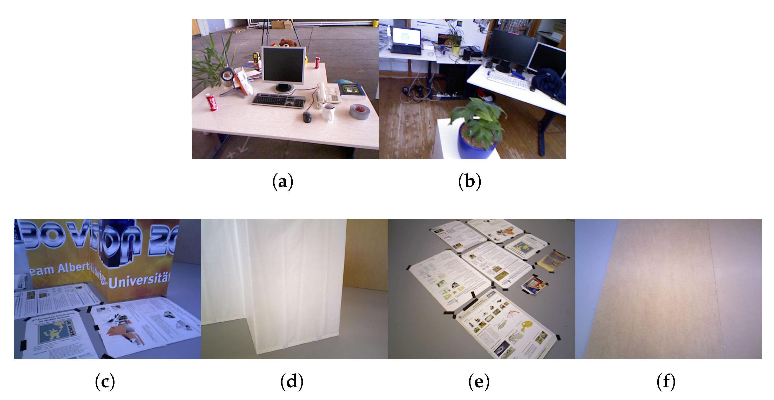
Our system was evaluated on six different sequences: fr1/plant, fr2/desk, fr3/structure-texture, fr3/structure-no texture, fr3/no structure-texture, and fr3/no structure-no texture. All these sequences were recorded with a handheld RGB-D Kinect sensor. Figure 3 shows the samples from the different sequences. Note that, in the second row, the conditions for visual pose estimation degrade progressively, ranging from the most favorable (Figure 3c, rich in texture, and structure) to the most challenging scenario (Figure 3f, lacking both structure and texture).

The metric used for the evaluation is the absolute trajectory error (ATE). It measures the global consistency of the estimated trajectory by computing the absolute distances between points in the estimated and ground-truth trajectories. It is a global measurement that requires both trajectories to be aligned in the same coordinate frame beforehand. One way to achieve this goal is to use the Horn method [34], which finds the rigid-body transformation $\mathbf{P}$ that maps the estimated trajectory ${\mathbf{S}}_{1:n}$ onto the ground truth trajectory ${\mathbf{Q}}_{1:n}$.

Given a rigid body transformation between the estimated trajectory and the ground truth data, the ATE at time step i can be computed as

$$AT{E}_i={\mathbf{Q}}_i^{-1}\mathbf{S}{\mathbf{P}}_i$$

(18)

then, the root mean squared error (RMSE) value of (18) is calculated using only the translational component.

$$AT{E}_{RMSE}=\sqrt{{\displaystyle \frac{1}{n}}{\sum }_{i=1}^n{∥trans\left({\mathbf{ATE}}_i\right)∥}^2}$$

(19)

Table 1. Results for the TUM RGB-D dataset.

Sequence	ATE RMSE [m]	ATE Mean [m]	ATE Median [m]	ATE Std [m]	ATE min [m]	ATE max [m]
fr1/plant	0.5567	0.4989	0.4895	0.2470	0.0185	1.0784
fr2/desk	0.4344	0.3900	0.3743	0.1914	0.0321	0.7947
fr3/s-t	0.0296	0.0275	0.0266	0.0108	0.0035	0.0619
fr3/s-Nt	0.1933	0.1795	0.1821	0.0715	0.0692	0.4366
fr3/Ns-t	0.0574	0.0529	0.0486	0.0222	0.0041	0.1155
fr3/Ns-Nt	0.3361	0.3121	0.2990	0.1246	0.1115	0.5243

Abbreviations: s-t: Structure–texture, Ns-t: No structure–texture, s-Nt: structure–no texture, Ns-Nt: No structure–no texture.

presents the absolute trajectory error (ATE) metrics for each of the sequences. The metrics were obtained using the automated evaluation tool provided with the dataset. The following analysis of Table 1 is supported by images depicting the trajectories generated throughout the experimental evaluations.

For sequences such as fr1/plant and fr2/desk, which contain rich visual features but involve severe perspective changes that challenge visual odometry systems, our proposal presents ATE values around 0.55 for fr1/plant and 0.43 for fr2/desk.

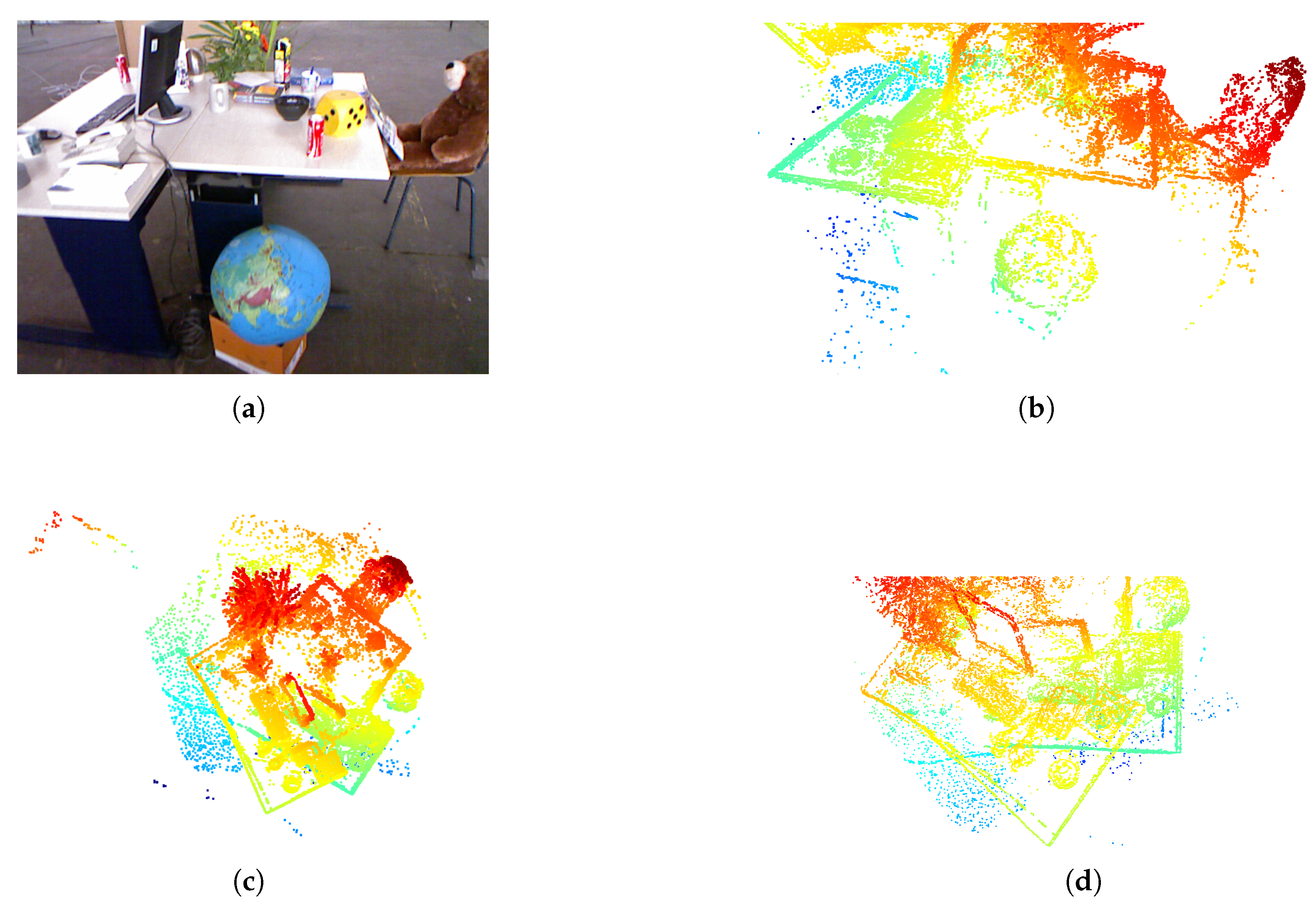
Figure 4 shows the different angles of the scene reconstruction for this sequence. Specifically, Figure 4c,d illustrate how the pose drift affects reconstruction. The yellow dots at the bottom-left corner of the desktop in Figure 4d represent the same region as the light blue/green dots on the left side of the image.

The structure–texture family of sequences presents increasingly difficult visual challenges for the pose estimation system. Similarly to the fr1/plant and fr2/desk, the fr3/structure–texture sequence provides images with rich structure and texture. As shown in Table 1, the system achieves its best results in this sequence, with an ATE RMSE of just 0.0296 m in the initial iteration and 0.0365 in the final iteration. This confirms the method’s capacity to provide highly accurate estimates when rich structure and texture are available. Figure 5a provides a visual comparison between the estimated trajectory and the ground truth.

In the fr3/no structure–texture sequence, a handheld camera moves along an approximately straight path through an area with posters placed on the floor. Due to the presence of these posters, the sequence contains a high level of texture but no structural information. During this evaluation, the system successfully recovers the camera trajectory, achieving an ATE RMSE of 0.0574 m.

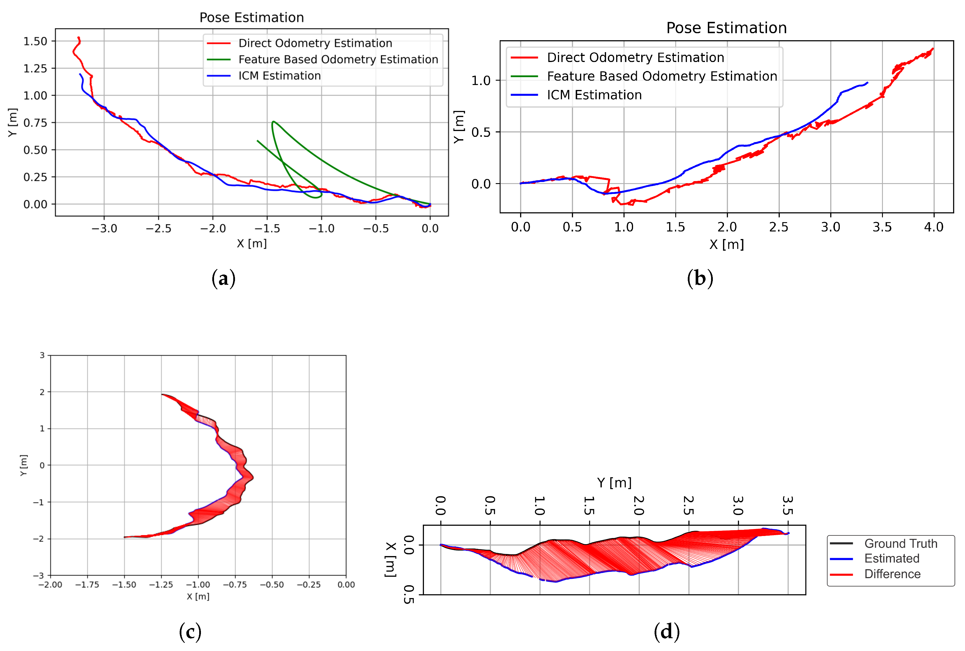
In texture-less sequences such as fr3/structure–no texture and fr3/no structure–no texture, the impact of the proposed adaptable odometry gain values becomes more apparent. For instance, in the case of the fr3/structure–no texture sequence (Figure 5b), the feature-based module can detect a few keypoints from image structure. However, the lack of texture leads to incorrect feature matching (i.e., wrong data association), resulting in poor pose estimation. As a consequence, the system assigns high uncertainty to the output of this module, which translates into a reduced gain. Then, its influence on the final optimization decreases, causing the system to rely more on direct odometry. This behavior of the system is visualized in Figure 6a), where the output of the two odometry systems and the output of the ICM module for the fr3/structure–no texture sequence is shown. It can be seen how the performance of the feature-based module decreases, and the ICM module decides to follow the direct odometry output. Table 1 reports an ATE RMSE of 0.19 m for this sequence, which can be visualized in Figure 6c.

A closer examination of the trajectories shown in Figure 5 reveals the impact of removing texture from the scene. It can be observed that, for a similar trajectory, the feature-based VO performs poorly in low-texture conditions. However, the adaptive gain scheme prevents tracking loss, at the cost of increased pose estimation error.

The fr3/no structure–no texture sequence represents a more extreme case. Almost no visual information is provided during the trajectory of the camera. The feature-based module consistently fails to obtain a pose estimate due to the complete absence of features (Figure 6b). In contrast, the direct method remains functional. Due to the contribution of the direct VO module and the proposed fusion system, tracking failure is successfully avoided, yielding a 0.3361 m ATE RMS error for the estimated trajectory. Figure 6d shows a comparison between the ground truth and estimated trajectories after alignment.

To date, the estimation error was assessed using a standard metric that measures the deviation between the computed trajectory and the ground truth. However, this metric does not allow for a qualitative comparison between the initial trajectory (iteration 0) and the final optimized trajectory (after N iterations). To address this, we need a metric sensitive to the properties optimized by the potential functions, which can effectively evaluate the improvements made over the N iterations. Thus, we propose using the point-wise mean cost computed at initialization and at the final optimization iteration:

$$\overline{C}={\displaystyle \frac{1}{N_c}}\sum _{i=1}^{N_c}{C}_i$$

(20)

The equation defines $\overline{C}$ as the average of the individual costs $C_i$ for all $N_c$ poses.

Table 2. Point-wise mean cost for de TUM RGB-D sequences.

Sequence	Mean Cost Value
fr1/plant it 0	$3.8419\times {10}^{-4}$
fr1/plant it N	$7.0364\times {10}^{-5}$
fr2/desk it 0	$5.0571\times {10}^{-5}$
fr2/desk it N	$8.2947\times {10}^{-6}$
fr3/s-t it 0	$1.5861\times {10}^{-4}$
fr3/s-t it N	$3.8727\times {10}^{-6}$
fr3/s-Nt it 0	$1.0226\times {10}^{-4}$
fr3/s-Nt it N	$4.6506\times {10}^{-6}$
fr3/Ns-t it 0	$7.5609\times {10}^{-4}$
fr3/Ns-t it N	$8.4838\times {10}^{-6}$
fr3/Ns-Nt it 0	$2.3016\times {10}^{-3}$
fr3/Ns-Nt it N	$3.8195\times {10}^{-5}$

presents the calculated mean cost for the TUM RGB-D sequences at iteration 0 and after N iterations.

A review of the table reveals a consistent reduction in the point-wise mean cost across all sequences. For each listed sequence, the mean cost at iteration ‘N’ is observed to be lower than the cost at iteration 0. This reduction indicates that the objective functions’ costs were effectively minimized by the optimization process. The consistent decrease demonstrates that providing the system with information about past and future time steps leads to an improvement in trajectory estimation.

3.2. Field Tests

Real-time experiments were also conducted using an RGB-D Intel Realsense D435-i camera as the system input (more info in https://www.intel.la/content/www/xl/es/products/sku/190004/intel-realsense-depth-camera-d435i/specifications.html, accessed on 29 August 2025). This device features a more advanced depth estimation module compared to the one used in the TUM dataset, resulting in fewer missing depth values. Furthermore, it provides pre-aligned color images and depth maps, eliminating the need for additional preprocessing by the programmer.

3.2.1. Indoor Test

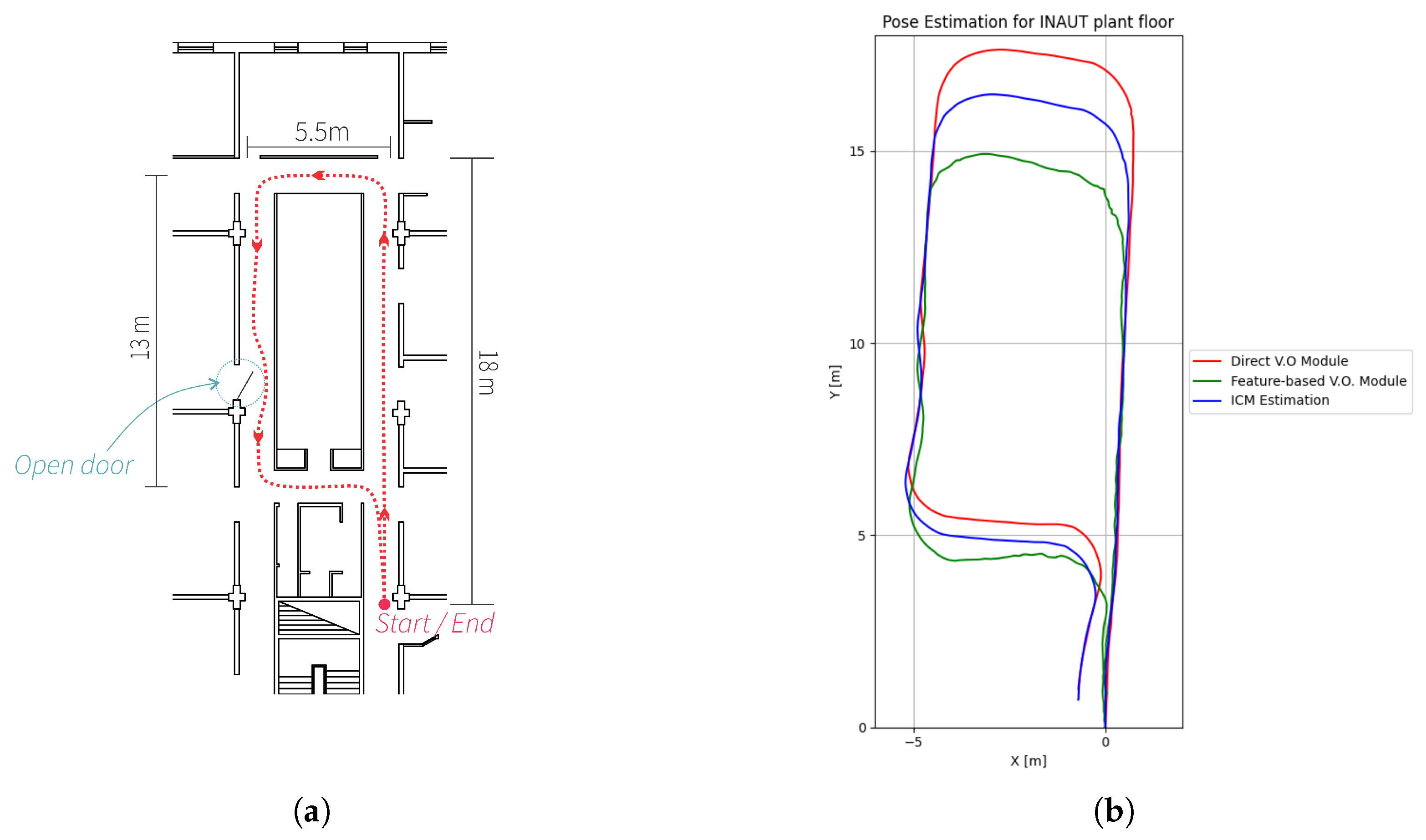
For this experiment, the camera was mounted on a wheeled platform and driven through the INAUT facilities. The path consisted of a single closed loop, starting and ending at the same position, but with opposite orientations. Figure 7a shows a simplified floor plan of the INAUT with an approximate sketch of the executed trajectory, while Figure 7b allows for a comparison between the estimated trajectories from direct odometry, feature-based odometry, and ICM.

The output of the feature-based odometry module, shown in Figure 7b, exhibits noise throughout the trajectory. This noise is effectively suppressed by the ICM, likely due to the effect of adaptive odometry gains. The resulting trajectory (in blue) is also metrically consistent with the expected path and the floor layout.

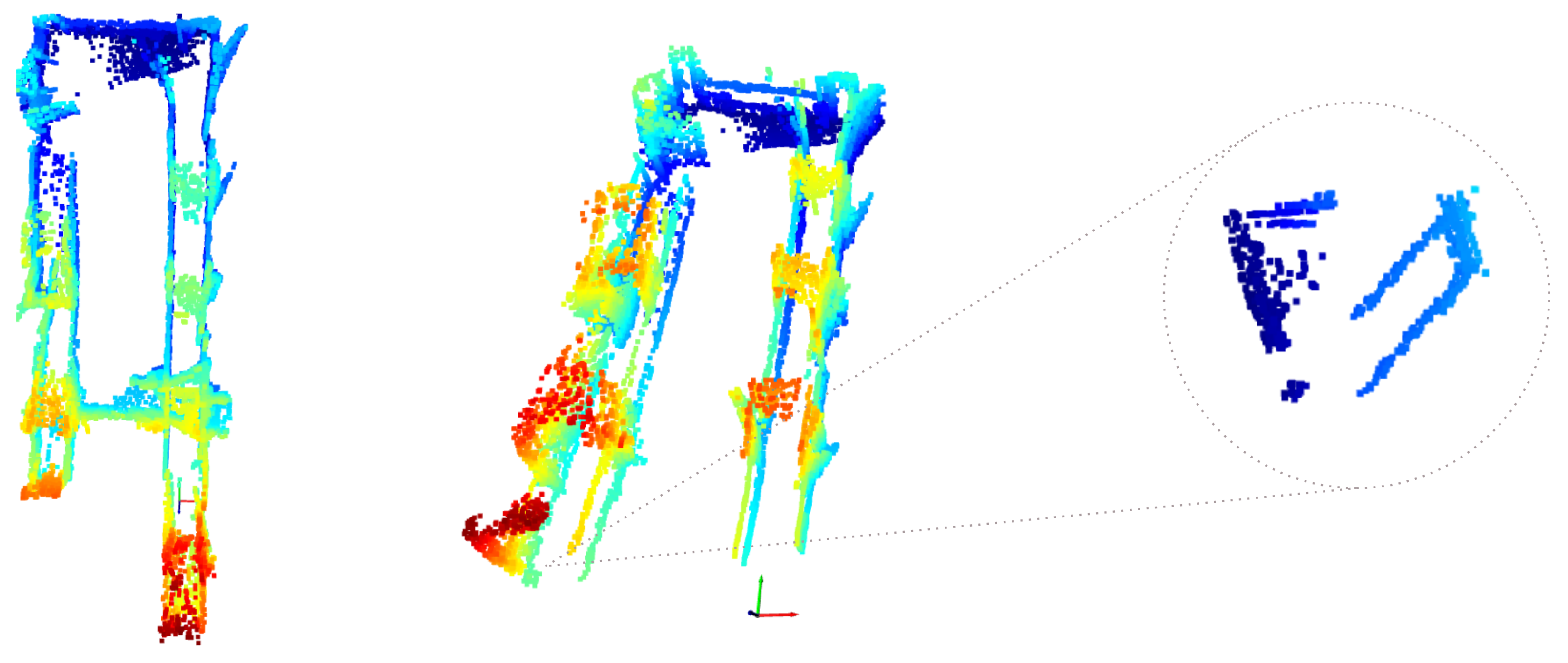
On the left side of Figure 8, a top view of the reconstructed scene for this experiment is shown. The central part of the figure shows the incremental construction of the global map, and a zoomed-in section depicts the local map representation used for computations at that specific point in the trajectory.

In the structured office environment, both systems maintain pose estimation without tracking failure. Compared to the outdoor scenario, the consistent artificial lighting minimizes the brightness changes between frames, reducing potential interference in the estimation process.

3.2.2. Outdoor Tests

The system’s performance was also evaluated in outdoor environments. Navigation in such scenarios poses additional challenges such as varying lighting conditions (shadows and high brightness), uneven terrain, and dynamic elements. In this experiment, the camera was mounted on the front of a Sero Electric Sedán [35] electric vehicle, which traversed an internal road on the FI-UNSJ campus at an average speed of 2.7 m/s. The purpose of this experiment is to assess the system’s ability to remain localized under typical outdoor conditions, such as those previously discussed. Estimation accuracy was previously validated using benchmark datasets with available ground truth.

Among the two odometry systems that feed the ICM module, the direct method is the one most affected in these environments. This is primarily due to its reliance on the photometric consistency assumption, which is often violated in the presence of lighting variations. To mitigate these effects, the selected points for motion estimation must be carefully selected. A pixel selection algorithm described in Appendix A is responsible for this task. It operates under two key principles: giving priority (when available) to high-gradient regions that correspond to structural elements in the scene, and ensuring the spatial distribution of points across the image to best capture the camera’s motion.

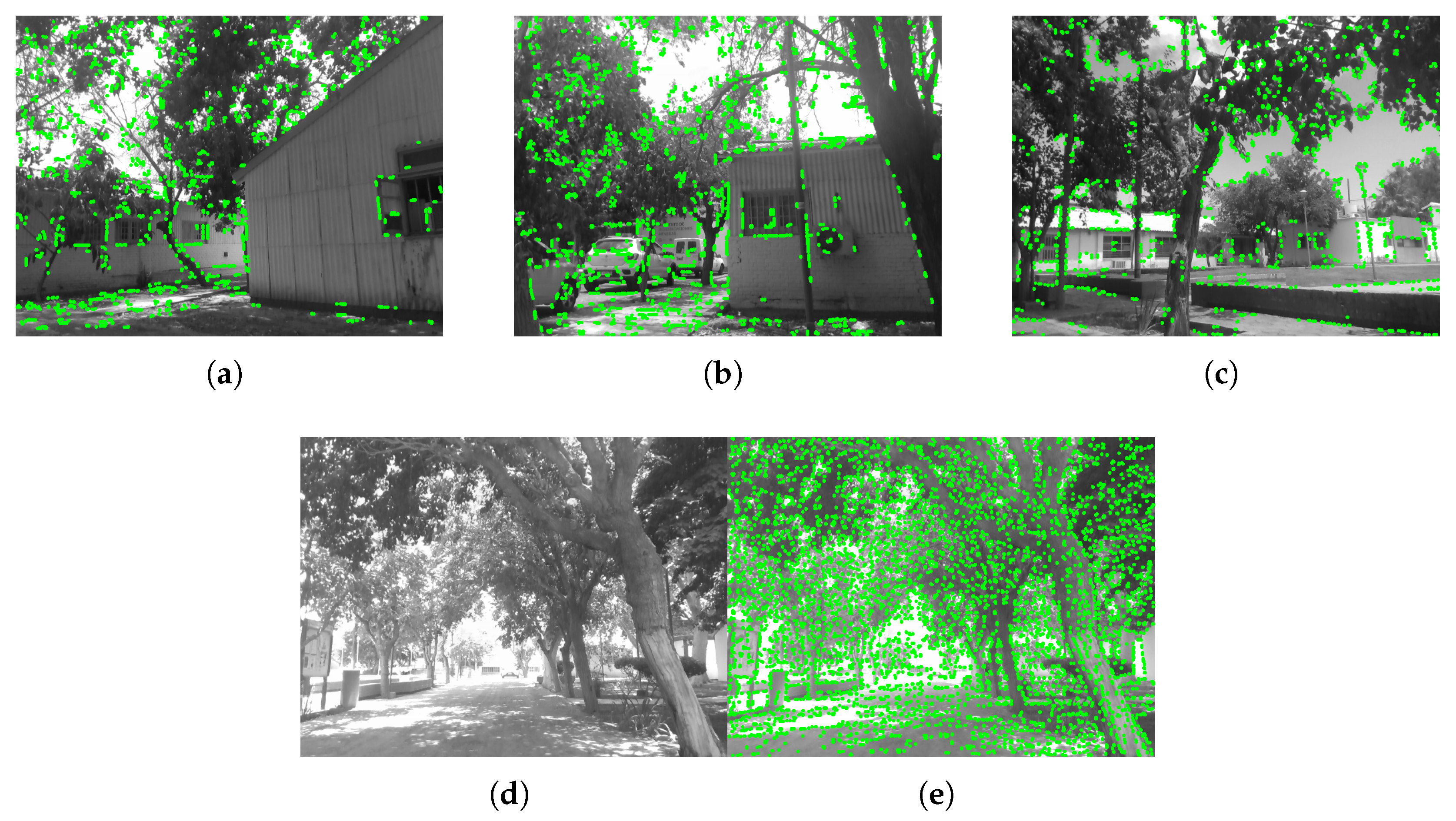
Sample frames from the outdoor experiments are shown in Figure 9. These grayscale images include green markers indicating the pixels selected for pose estimation. Each frame illustrates scenes with strong lighting contrast caused by sunlight passing through foliage and reflecting off building walls. If the algorithm were to select points solely based on gradient magnitude, they would be concentrated in areas of highest contrast—typically at the boundaries between bright sky and dark foliage. However, the system reduces the number of extracted points and prioritizes structured elements such as window frames, tree trunks, and lampposts, as can be seen in Figure 9a–c.

This response is due to the internal use of texture-based criteria within the point extraction module, enabling it to disregard areas with rapid grayscale changes—such as foliage—that are less reliable for tracking. Nevertheless, due to the trade-off between performance and computational efficiency, the system may still select points in suboptimal regions during outdoor scenarios. Despite this, it consistently ensures a spatially balanced distribution of points and avoids selecting from low-texture areas such as sky, grass, or planar surfaces.

Real-world experiments may present challenging scenarios like that shown in Figure 9d. In addition to regions with high brightness, the areas that could potentially provide structural information exhibit very low gradients (i.e., nearly uniform grayscale levels). In such scenarios, the system compensates by distributing selected points across the image, thereby preserving the tracking performance throughout the sequence.

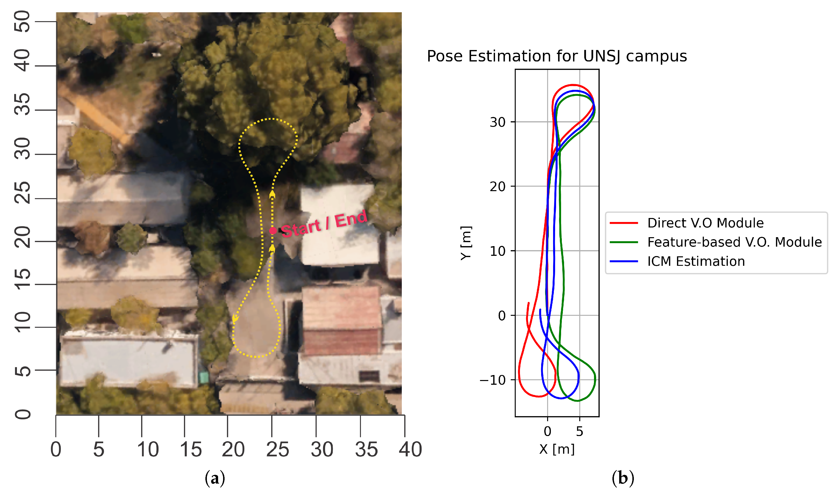
The outdoor test itself involved following a round-trip path along one of the internal streets of the UNSJ campus, as illustrated in Figure 10a. The recovered trajectory after the test is shown in Figure 10b. Both odometry systems exhibit different biases when estimating the turning angle, which affects the final trajectory. However, since the proposed method combines these measurements with other sources of information, the proposed method yields a trajectory that is both metrically accurate and morphologically aligned with the actual path followed.

4. Discussion

Most visual odometry systems reported in the state of the art have been designed to operate entirely within a single paradigm, either by means of direct methods or by means of indirect (feature-based) methods. The approach presented in this work was conceived to break such a dichotomy by employing both methods simultaneously within a unified framework, thereby taking advantage of the complementary benefits of each system while at the same time reducing their respective weaknesses. Special emphasis was placed on this latter point, in order to ensure the continuity of pose tracking even in situations in which one of the odometry systems failed completely.

In order to achieve this objective, a modular scheme with adaptable gains was implemented, whose values are automatically adjusted according to the estimation uncertainty provided by each of the odometry systems. The action of these gains makes it possible to regulate the influence of the potential functions associated with them during the optimization process performed by the ICM algorithm.

As illustrated by the results in Figure 6, the system demonstrates robustness against degradation or loss of the feature-based odometry. In such scenarios, the system adapts to feature-deprived environments by relying on the odometry obtained from the direct system. Even under these conditions, the recovered trajectory remains close to the ground truth.

Another challenge addressed during the evaluation of the system was the execution of field tests, whose principal aim was to validate the functioning of the system under a variety of lighting conditions. In the indoor office environment, artificial lighting remained constant, while in the outdoor environment, certain areas presented high-contrast image regions. This latter condition is especially problematic for direct systems, because information can be drawn from high-gradient zones (for instance, where sunlight filters through foliage) that fail to reflect the actual structure of the image and thus impede accurate estimation. For that reason, an adaptive pixel selection scheme was implemented, which allows the system to search for those points in the image that best represent its structure. The results obtained confirm that incorporating such a scheme into the system offers a decisive advantage in preventing the direct system from losing localization. Overall, the results confirm that the proposed system is capable of maintaining localization in low-texture environments, which represent particularly adverse conditions for feature-based odometry systems.

The main limitation of the presented approach lies in the fact that ICM operates iteratively, commencing with an initial estimate of the environment map and robot trajectory. Subsequently, it refines these estimates through successive iterations until convergence to a solution is achieved. While these results represent an improvement over the initial estimates and can thus enhance the output of the system, ICM’s performance is highly dependent on the quality of its initialization.

The main limitation of the proposed approach arises from the fact that the ICM algorithm operates in an iterative manner, beginning with an initial estimate of both the environment map and the robot trajectory. These estimates are subsequently refined through successive iterations until a convergence criterion is met. Although the iterative process consistently yields results that improve the initial estimates and thereby enhance the overall output of the system, the quality of the final solution remains strongly dependent on the accuracy of the initialization. Inadequate initial estimates could lead the algorithm to converge to suboptimal local maxima.

Future research directions include the incorporation of a loop closure detection system and the development of a potential function that allows the information obtained from such a system to be incorporated into the optimization process. Furthermore, although the present work focuses on the fusion of different visual odometry systems, it is of particular interest to carry out fusion tests with odometries coming from sensors of another nature, such as LiDAR sensors or wheel odometry from the robot.

5. Conclusions

This article introduces a novel modular fusion architecture designed for 6-DoF camera pose estimation, integrating outputs from both direct and feature-based visual odometry (VO) methods. Incoming RGB-D frames are concurrently processed by a feature-based VO module and a direct VO module, each generating independent pose estimations. These estimations are subsequently fed into the Iterated Conditional Modes (ICMs) algorithm as odometry potentials, which are then fused with a local map and a set of observations to yield a refined pose estimate.

The proposed novel design improves the system robustness against tracking loss in visually degraded or low-texture environments due to the effect of two key tools: first, a pixel selection strategy that ensures that the selected pixels for the direct VO module are those that best capture the camera’s motion. Second, the system dynamically adjusts the influence of each odometry source based on its estimated uncertainty.

The comprehensive validation of the proposed method was conducted through experiments on the TUM RGB-D benchmark and real-world field tests in both indoor and outdoor settings, demonstrating its ability to maintain stable tracking in structured, semi-structured, and unstructured environments.

Despite its inherent computational efficiency and straightforward implementation, the ICM algorithm has not been widely utilized in visual mobile robot navigation applications. The contributions presented herein offer a foundation for deploying reliable autonomous localization and mapping solutions in practical mobile robotics, such as electric vehicles, where the tracking loss is unacceptable and environmental conditions are frequently challenging for conventional VO systems.

References

1. Yang, K.; Cheng, Y.; Chen, Z.; Wang, J. Slam meets nerf: A survey of implicit slam methods. World Electr. Veh. J. 2024, 15, 85. [Google Scholar] [CrossRef]
2. Lluvia, I.; Lazkano, E.; Ansuategi, A. Active Mapping and Robot Exploration: A Survey. Sensors 2021, 21, 2445. [Google Scholar] [CrossRef]
3. Placed, J.A.; Strader, J.; Carrillo, H.; Atanasov, N.; Indelman, V.; Carlone, L.; Castellanos, J.A. A survey on active simultaneous localization and mapping: State of the art and new frontiers. IEEE Trans. Robot. 2023, 39, 1686–1705. [Google Scholar] [CrossRef]
4. Gaia, J.; Orosco, E.; Rossomando, F.; Soria, C. Mapping the Landscape of SLAM Research: A Review. IEEE Lat. Am. Trans. 2023, 21, 1313–1336. [Google Scholar] [CrossRef]
5. Li, Y.; An, J.; He, N.; Li, Y.; Han, Z.; Chen, Z.; Qu, Y. A Review of Simultaneous Localization and Mapping Algorithms Based on Lidar. World Electr. Veh. J. 2025, 16, 56. [Google Scholar] [CrossRef]
6. Wu, D.; Ma, Z.; Xu, W.; He, H.; Li, Z. Visual Odometry Based on Improved Oriented Features from Accelerated Segment Test and Rotated Binary Robust Independent Elementary Features. World Electr. Veh. J. 2024, 15, 123. [Google Scholar] [CrossRef]
7. Scaramuzza, D.; Fraundorfer, F. Visual odometry [tutorial]. IEEE Robot. Autom. Mag. 2011, 18, 80–92. [Google Scholar] [CrossRef]
8. Tardif, J.P.; Pavlidis, Y.; Daniilidis, K. Monocular visual odometry in urban environments using an omnidirectional camera. In Proceedings of the 2008 IEEE/RSJ International Conference on Intelligent Robots and Systems, Nice, France, 22–26 September 2008; pp. 2531–2538. [Google Scholar] [CrossRef]
9. Bescos, B.; Fácil, J.M.; Civera, J.; Neira, J. DynaSLAM: Tracking, mapping, and inpainting in dynamic scenes. IEEE Robot. Autom. Lett. 2018, 3, 4076–4083. [Google Scholar] [CrossRef]
10. Engel, J.; Schöps, T.; Cremers, D. LSD-SLAM: Large-scale direct monocular SLAM. In Proceedings of the European Conference on Computer Vision, Zurich, Switzerland, 6–12 September 2014; pp. 834–849. [Google Scholar] [CrossRef]
11. Engel, J.; Stückler, J.; Cremers, D. Large-scale direct SLAM with stereo cameras. In Proceedings of the 2015 IEEE/RSJ International Conference on Intelligent Robots and Systems (IROS), Hamburg, Germany, 28 September–2 October 2015; pp. 1935–1942. [Google Scholar] [CrossRef]
12. Engel, J.; Koltun, V.; Cremers, D. Direct sparse odometry. IEEE Trans. Pattern Anal. Mach. Intell. 2017, 40, 611–625. [Google Scholar] [CrossRef] [PubMed]
13. Zhu, Z.; Peng, S.; Larsson, V.; Xu, W.; Bao, H.; Cui, Z.; Oswald, M.R.; Pollefeys, M. Nice-slam: Neural implicit scalable encoding for slam. In Proceedings of the IEEE/CVF Conference on Computer Vision and Pattern Recognition, New Orleans, LA, USA, 18–24 June 2022; pp. 12786–12796. [Google Scholar]
14. Gao, X.; Wang, R.; Demmel, N.; Cremers, D. LDSO: Direct sparse odometry with loop closure. In Proceedings of the 2018 IEEE/RSJ International Conference on Intelligent Robots and Systems (IROS), Madrid, Spain, 1–5 October 2018; pp. 2198–2204. [Google Scholar] [CrossRef]
15. Yang, N.; Stumberg, L.v.; Wang, R.; Cremers, D. D3vo: Deep depth, deep pose and deep uncertainty for monocular visual odometry. In Proceedings of the IEEE/CVF Conference on Computer Vision and Pattern Recognition, Seattle, WA, USA, 13–19 June 2020; pp. 1281–1292. [Google Scholar] [CrossRef]
16. Matsuki, H.; Murai, R.; Kelly, P.H.; Davison, A.J. Gaussian splatting slam. In Proceedings of the IEEE/CVF Conference on Computer Vision and Pattern Recognition, Seattle, WA, USA, 16–22 June 2024; pp. 18039–18048. [Google Scholar]
17. Schlegel, D.; Grisetti, G. Visual localization and loop closing using decision trees and binary features. In Proceedings of the 2016 IEEE/RSJ International Conference on Intelligent Robots and Systems (IROS), Daejeon, Republic of Korea, 9–14 October 2016; pp. 4616–4623. [Google Scholar] [CrossRef]
18. Nobis, F.; Papanikolaou, O.; Betz, J.; Lienkamp, M. Persistent Map Saving for Visual Localization for Autonomous Vehicles: An ORB-SLAM 2 Extension. In Proceedings of the 2020 Fifteenth International Conference on Ecological Vehicles and Renewable Energies (EVER), Monte-Carlo, Monaco, 10–12 September 2020; pp. 1–9. [Google Scholar] [CrossRef]
19. Elvira, R.; Tardós, J.D.; Montiel, J.M. ORBSLAM-Atlas: A robust and accurate multi-map system. In Proceedings of the 2019 IEEE/RSJ International Conference on Intelligent Robots and Systems (IROS), Macau, China, 3–8 November 2019; pp. 6253–6259. [Google Scholar] [CrossRef]
20. Li, J.; Wang, X.; Li, S. Spherical-model-based SLAM on full-view images for indoor environments. Appl. Sci. 2018, 8, 2268. [Google Scholar] [CrossRef]
21. Campos, C.; Elvira, R.; Rodríguez, J.J.G.; Montiel, J.M.; Tardós, J.D. ORB-SLAM3: An Accurate Open-Source Library for Visual, Visual–Inertial, and Multimap SLAM. IEEE Trans. Robot. 2021, 37, 1874–1890. [Google Scholar] [CrossRef]
22. Mur-Artal, R.; Montiel, J.M.M.; Tardos, J.D. ORB-SLAM: A versatile and accurate monocular SLAM system. IEEE Trans. Robot. 2015, 31, 1147–1163. [Google Scholar] [CrossRef]
23. Folkesson, J.; Christensen, H. Graphical SLAM-a self-correcting map. In Proceedings of the IEEE International Conference on Robotics and Automation, New Orleans, LA, USA, 26 April–1 May 2004; Proceedings, ICRA’04. Volume 1, pp. 383–390. [Google Scholar]
24. Grisetti, G.; Kümmerle, R.; Stachniss, C.; Burgard, W. A tutorial on graph-based SLAM. IEEE Intell. Transp. Syst. Mag. 2010, 2, 31–43. [Google Scholar] [CrossRef]
25. Akai, N.; Akagi, Y.; Hirayama, T.; Morikawa, T.; Murase, H. Detection of localization failures using Markov random fields with fully connected latent variables for safe LiDAR-based automated driving. IEEE Trans. Intell. Transp. Syst. 2022, 23, 17130–17142. [Google Scholar] [CrossRef]
26. Kindermann, R.; Snell, J.L. Markov Random Fields and Their Applications; American Mathematical Society: Providence, RI, USA, 1980; Volume 1. [Google Scholar]
27. Jadaliha, M.; Choi, J. Fully Bayesian simultaneous localization and spatial prediction using Gaussian Markov random fields (GMRFs). In Proceedings of the 2013 American Control Conference, Washington, DC, USA, 17–19 June 2013; pp. 4592–4597. [Google Scholar]
28. Wang, C.; Li, T.; Meng, M.Q.H.; De Silva, C. Efficient mobile robot exploration with Gaussian Markov random fields in 3D environments. In Proceedings of the 2018 IEEE International Conference on Robotics and Automation (ICRA), Brisbane, QLD, Australia, 21–25 May 2018; pp. 5015–5021. [Google Scholar]
29. Gimenez, J.; Amicarelli, A.; Toibero, J.M.; di Sciascio, F.; Carelli, R. Iterated conditional modes to solve simultaneous localization and mapping in Markov random fields context. Int. J. Autom. Comput. 2018, 15, 310–324. [Google Scholar] [CrossRef]
30. Gimenez, J.; Amicarelli, A.; Toibero, J.M.; di Sciascio, F.; Carelli, R. Continuous probabilistic SLAM solved via iterated conditional modes. Int. J. Autom. Comput. 2019, 16, 838–850. [Google Scholar] [CrossRef]
31. Besag, J. On the statistical analysis of dirty pictures. J. R. Stat. Soc. Ser. B Stat. Methodol. 1986, 48, 259–279. [Google Scholar] [CrossRef]
32. Jaime, F.; Marzola, T.; Baldoni, M.; Mattoccia, S. HoloSLAM: A novel approach to virtual landmark-based SLAM for indoor environments. SN Comput. Sci. 2024, 5, 469. [Google Scholar]
33. Sturm, J.; Engelhard, N.; Endres, F.; Burgard, W.; Cremers, D. A benchmark for the evaluation of RGB-D SLAM systems. In Proceedings of the 2012 IEEE/RSJ International Conference on Intelligent Robots and Systems, Vilamoura-Algarve, Portugal, 7–12 October 2012; pp. 573–580. [Google Scholar]
34. Horn, B.K. Closed-form solution of absolute orientation using unit quaternions. J. Opt. Soc. Am. 1987, 4, 629–642. [Google Scholar] [CrossRef]
35. Sero Electric Sedan Electric Vehicle. Available online: https://www.seroelectric.com/modelo-sedan/ (accessed on 7 May 2025).
36. Haralick, R.M.; Shanmugam, K.; Dinstein, I.H. Textural features for image classification. IEEE Trans. Syst. Man, Cybern. 1973, 6, 610–621. [Google Scholar] [CrossRef]
37. Galloway, M.M. Texture analysis using grey level run lengths. Nasa Sti/Recon Tech. Rep. N 1974, 75, 18555. [Google Scholar]
Figure 1. System overview as a block diagram. The inputs x ^ t f e a t and x ^ t d i r are interpreted as odometry measurements by the ICM module, which additionally receives observation data and the local map m for pose estimation.
Wevj 16 00510 g001
Figure 2. Two−phase process of the ICM Algorithm. (Left) The initialization phase (iteration 0) determines the current system pose using past and present data. (Right) N iterations if the ICM algorithm are performed to refine the trajectory estimates. To update a state at a given time step, this process leverages all available information, including past and future states.
Wevj 16 00510 g002
Figure 3. Samples of the color frames of the TUM RGB-D dataset for the following sequences: (a) fr2/desk. (b) fr1/plant. (c) fr3/structure-texture. (d) fr3/structure-no texture. (e) fr3/no structure-texture. (f) fr3/no structure-no texture.
Wevj 16 00510 g003
Figure 4. Reconstruction details for the fr2/desk sequence. (a) Reference RGB frame. (b) Reconstruction taken from a similar point of view. (c) Top view of the final global map for the sequence. (d) Detail showing the drift in the reconstruction.
Wevj 16 00510 g004
Figure 5. Pose estimation results for the structure–texture sequences. (a) fr3/structure–texture, (b) fr3/structure–no texture.
Wevj 16 00510 g005
Figure 6. Internal trajectories recovered by the VO systems and the ICM module for the TUM RGB-D sequences: (a) fr3/structure–no texture. (b) fr3/no structure–no texture. (c,d) Aligned ground truth and estimated trajectories for the fr3/structure–no texture and fr3/no structure–no texture sequences, respectively. Note that, even when feature-based odometry fails, the system is still able to perform pose estimation due to the adaptable gain scheme.
Wevj 16 00510 g006
Figure 7. (a) Approximated trajectory followed within the INAUT facilities. (b) Trajectory recovered by both VO systems and the ICM module (system output).
Wevj 16 00510 g007
Figure 8. (Left): Final global map of the facilities of the Instituto de Automática after iteration 0 is completed. (Center): Snapshot of the global map at an intermediate stage of the initialization process. (Right): Detail of the local map m , built with previous observations.
Wevj 16 00510 g008
Figure 9. Sample images from the outdoor tests. Figures (ac) show how the internal pixel selection algorithm seeds points for pose estimation (green) under normal conditions. Figures (d,e) depict a very challenging scenario with very low gray-level difference in possible areas of interest and high gradient areas due to illumination changes.
Wevj 16 00510 g009
Figure 10. Outdoor tests: (a) Approximated trajectory followed by the electric vehicle on the UNSJ campus. (b) Results for ICM iteration 0.
Wevj 16 00510 g010