Author Contributions
Conceptualization, A.D., R.B., J.G. and C.-G.Q.; Data curation, A.D. and R.B.; Formal analysis, A.D. and R.B.; Funding acquisition, A.D., R.B., J.G. and C.-G.Q.; Investigation, A.D. and R.B.; Methodology, A.D., R.B., J.G. and C.-G.Q.; Project administration, R.B., J.G. and C.-G.Q.; Resources, A.D., R.B., J.G. and C.-G.Q.; Software, A.D. and R.B.; Supervision, R.B., J.G. and C.-G.Q.; Validation, A.D., R.B. and C.-G.Q.; Visualization, A.D.; Writing—original draft, A.D.; Writing—review and editing, A.D., R.B. and C.-G.Q. All authors have read and agreed to the published version of the manuscript.
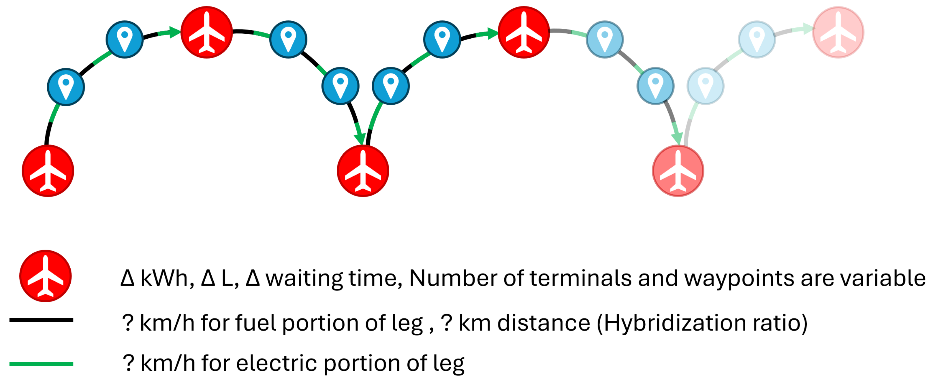
Figure 1.
Visual representation of an instance of the S-FRHACP-VS and its decision variables. The fixed route is composed of a series of terminals (typically airports) with waypoints splitting the route between two terminals. The decision variables are split between terminal’s decisions (charging quantity, refueling quantity, and waiting time) and leg’s decisions (flight speed on the fuel and electric portion of the leg, and hybridization ratio).
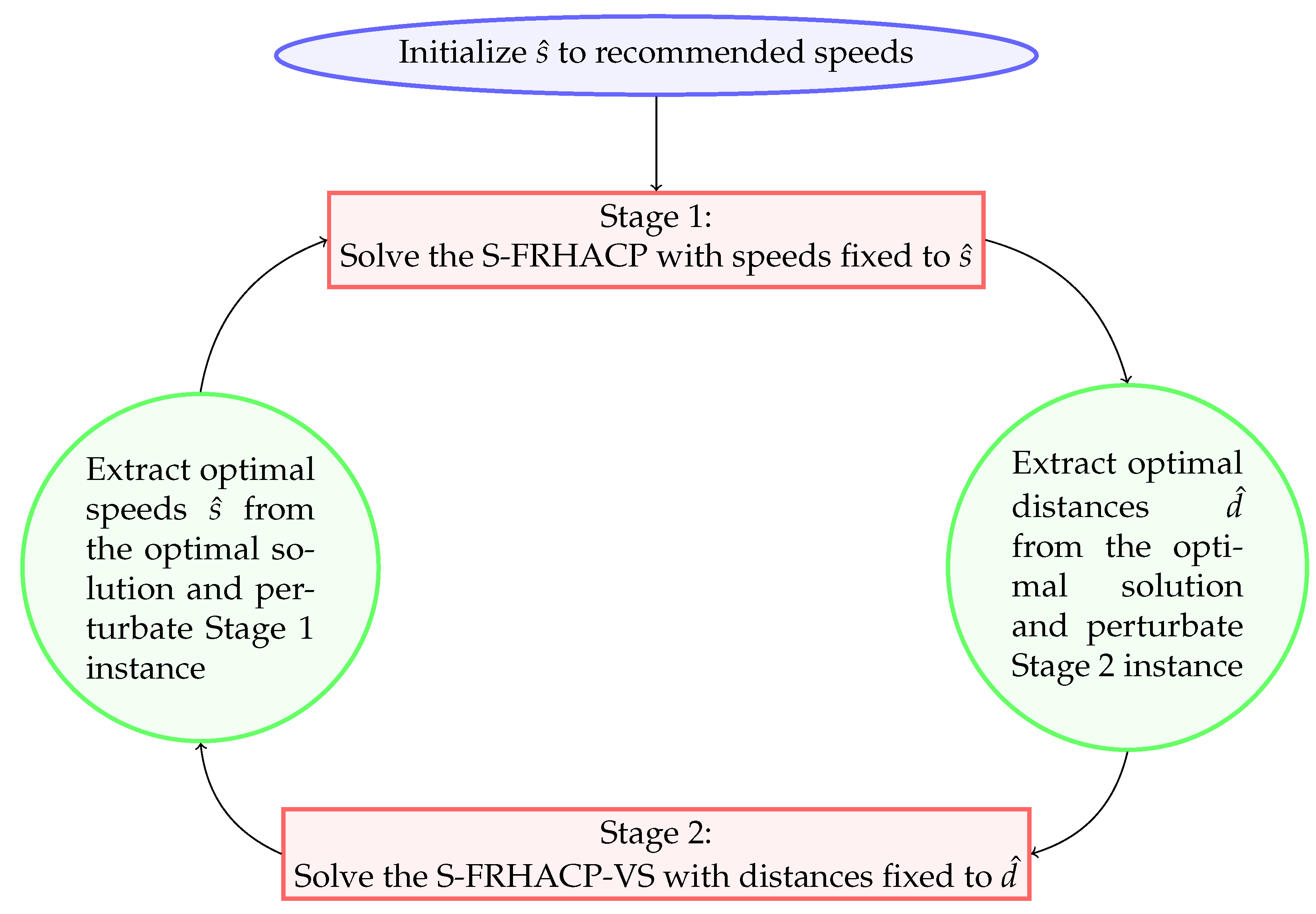
Figure 2.
Flowchart representing the Iterative Two-Stage MIP Heuristic for the S-FRHACP-VS. The heuristic starts by fixing the speeds to the initial recommended speeds, then solves the resulting S-FRHACP instance in Stage 1. The optimal distances are extracted from the optimal solution of Stage 1. Then, the heuristic solves the S-FRHACP-VS where the distances are fixed to the extracted distances (using the Stage 2 MIP model). Finally, the optimal speeds are extracted from the optimal solution of Stage 2 and the process can then be repeated using the newly extracted speeds until convergence.
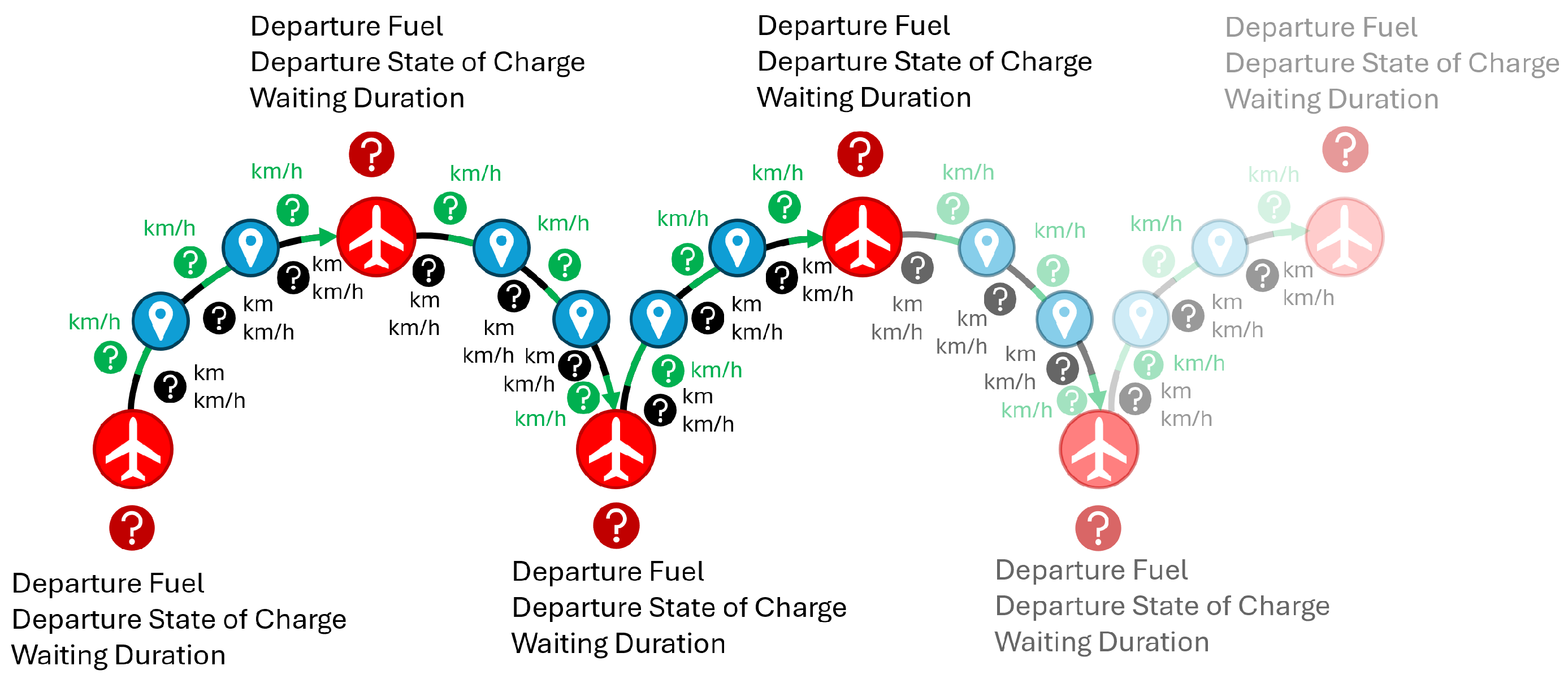
Figure 3.
Visual representation of how the genetic algorithm genes relate to an instance of the S-FRHACP-VS. The first variables are at the starting terminal and they represent charging, refueling, and waiting decisions. During the flights, the genes represent the hybridization ratio (km), the chosen flight speed for the fuel portion of the leg, and the flight speed electric portion of the leg.
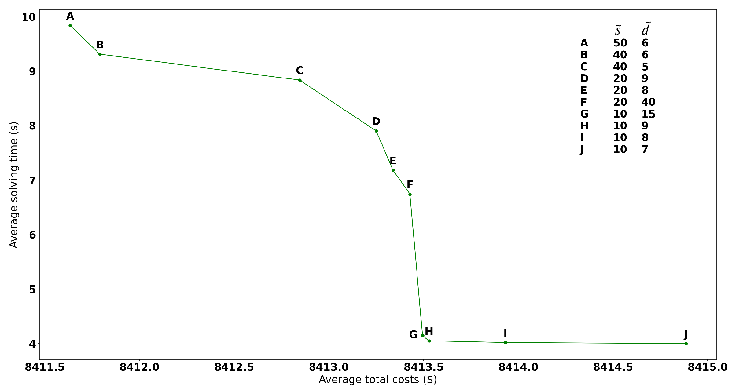
Figure 4.
Resulting Pareto front for the DP and DP+GD approaches on the training set with tested hyperparameter combinations. Each point from A to J represents a combination of state of charge sampled () and maximal number of iterations of Brent’s algorithm () that dominates either on average total costs or average solving time on the training set. This Pareto front can then be used to choose a combination of hyperparameters to use on the test set (Point G).
Figure 5.
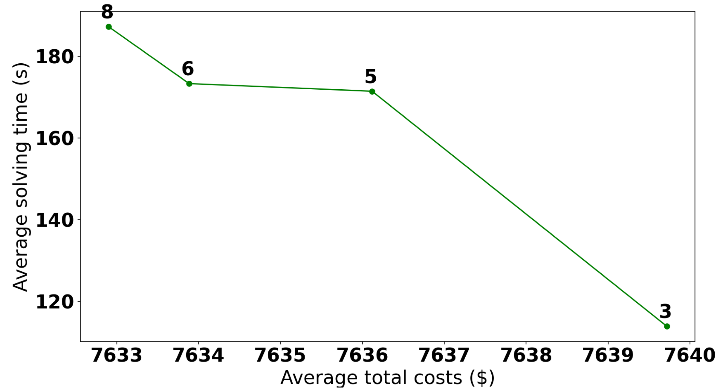
Resulting Pareto front for the Stage 2 MIP model on the training set with tested hyperparameter values. Each point represents a value of the number of points in the grid sampling used to approximate the energy consumption functions for the durations () that dominates either on average total costs or average solving time on the training set. This value is shown above each point in the plot. This Pareto front can then be used to choose the value of this hyperparameter to use on the test set (3).
Figure 6.
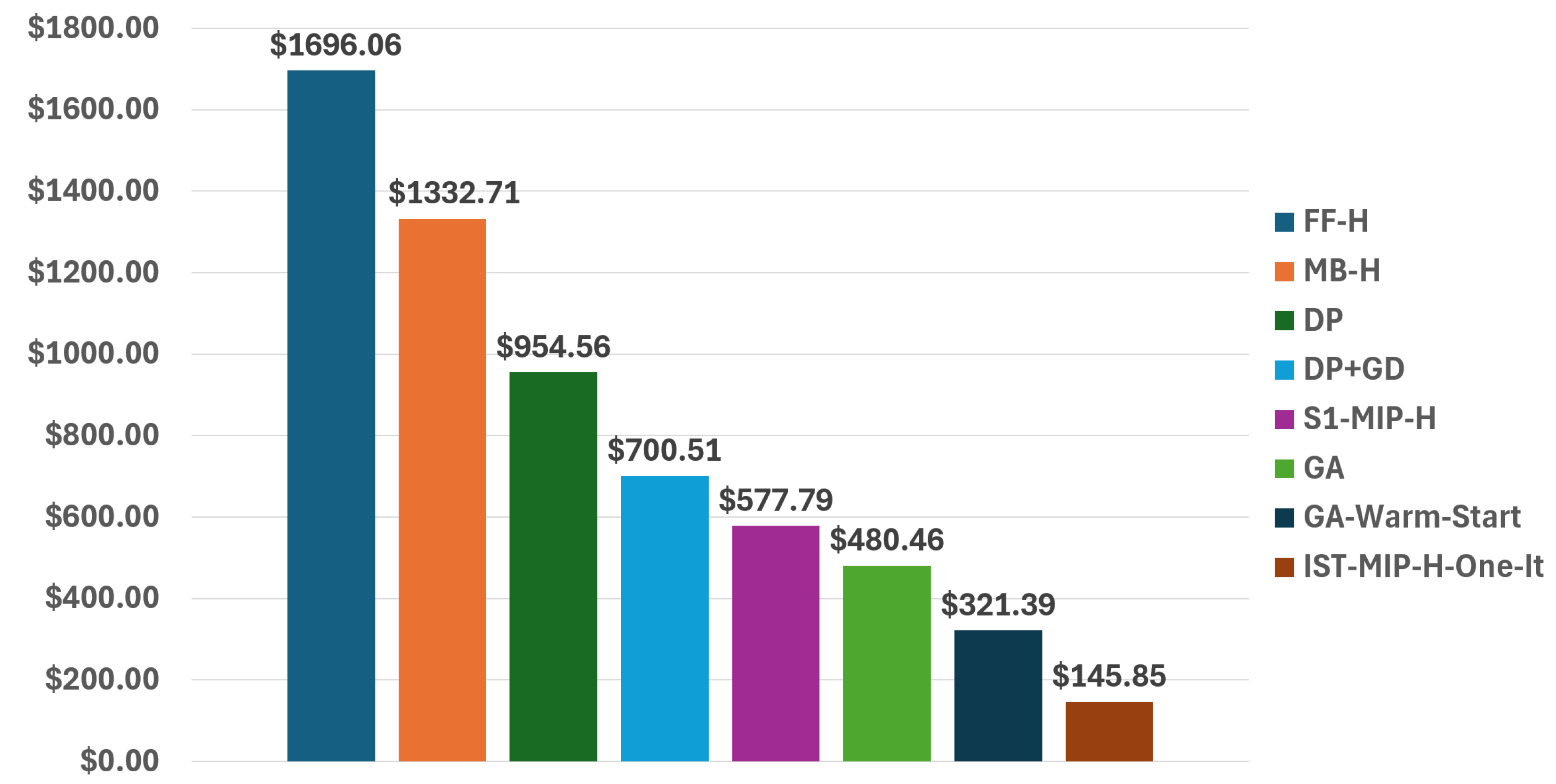
Average increase in total costs over the test instances of each approach in comparison with the ITS-MIP-H approach.
Figure 6.
Average increase in total costs over the test instances of each approach in comparison with the ITS-MIP-H approach.
Figure 7.
Average percentage increase in total costs over the test instances of each approach in comparison with the ITS-MIP-H approach.
Figure 7.
Average percentage increase in total costs over the test instances of each approach in comparison with the ITS-MIP-H approach.
Figure 8.
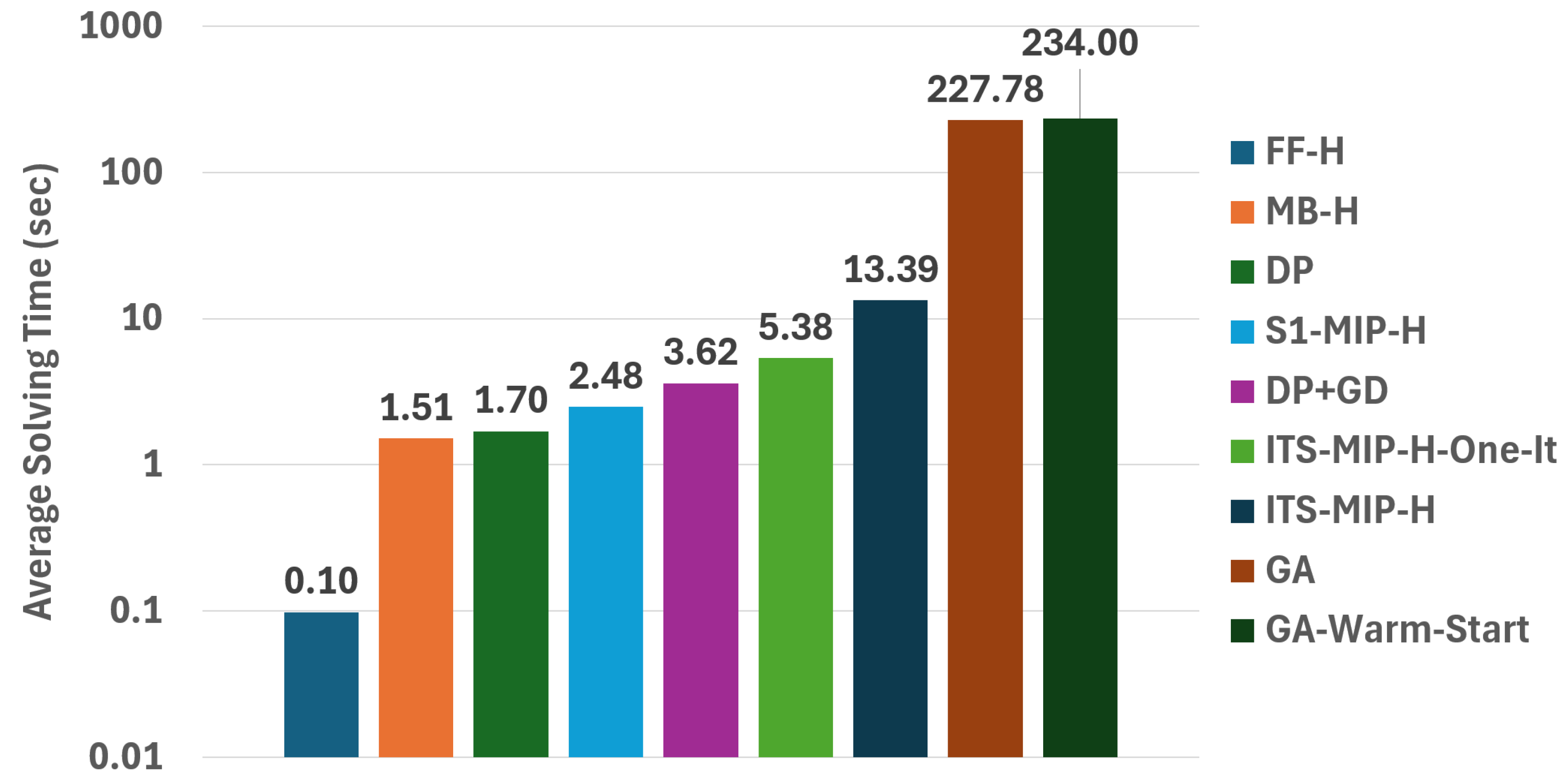
Semi-log plot of the average solving time (s) of each approach over the test instances.
Figure 8.
Semi-log plot of the average solving time (s) of each approach over the test instances.
Figure 9.
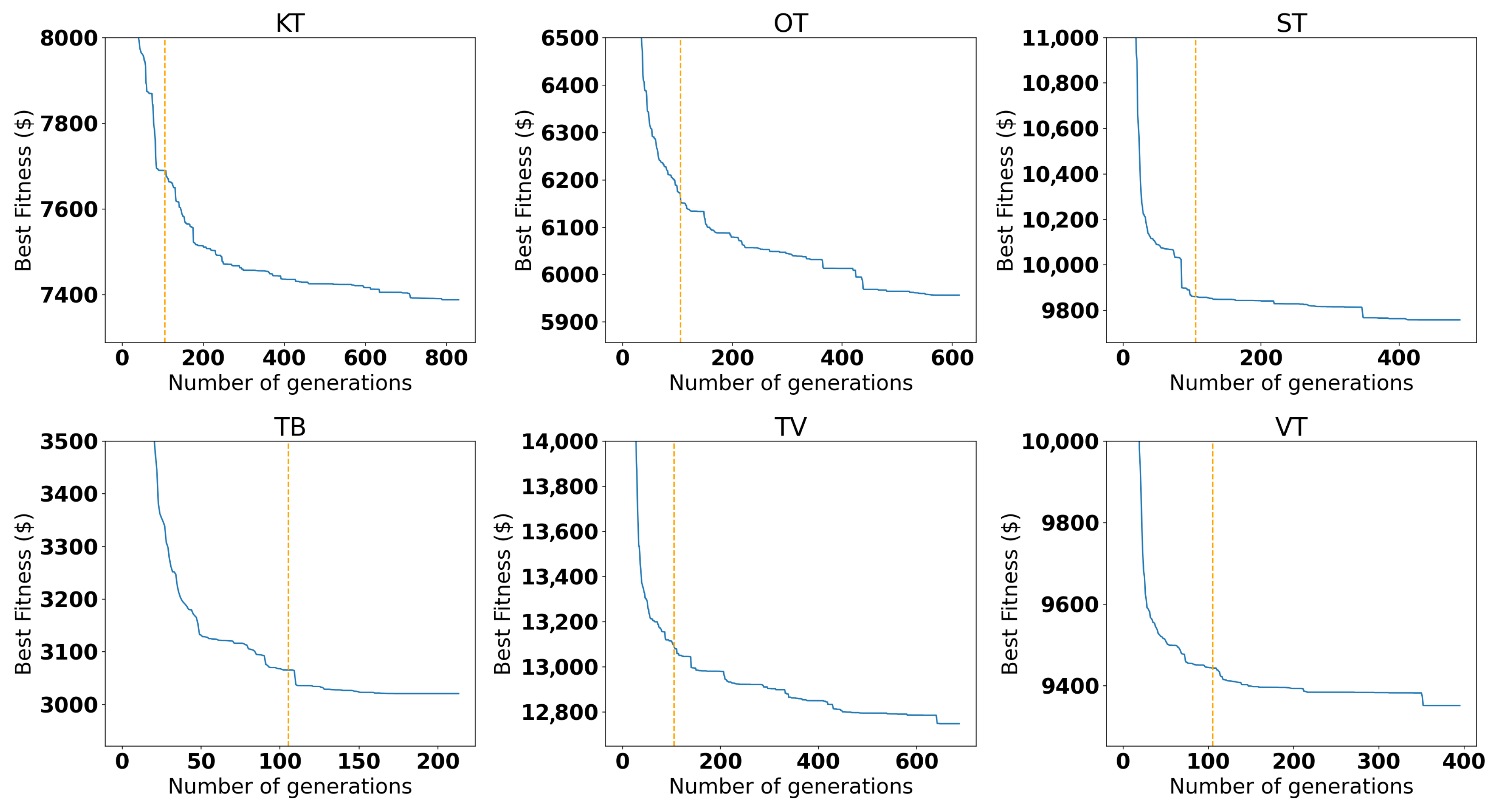
Convergence plot of the GA approach for each instance. The dashed orange line represents the best solution obtained at the generation limit (15,000 individuals, which represents 105 generations). The Y axis has been cropped, since the first generations have high-value best individuals.
Figure 9.
Convergence plot of the GA approach for each instance. The dashed orange line represents the best solution obtained at the generation limit (15,000 individuals, which represents 105 generations). The Y axis has been cropped, since the first generations have high-value best individuals.
Figure 10.
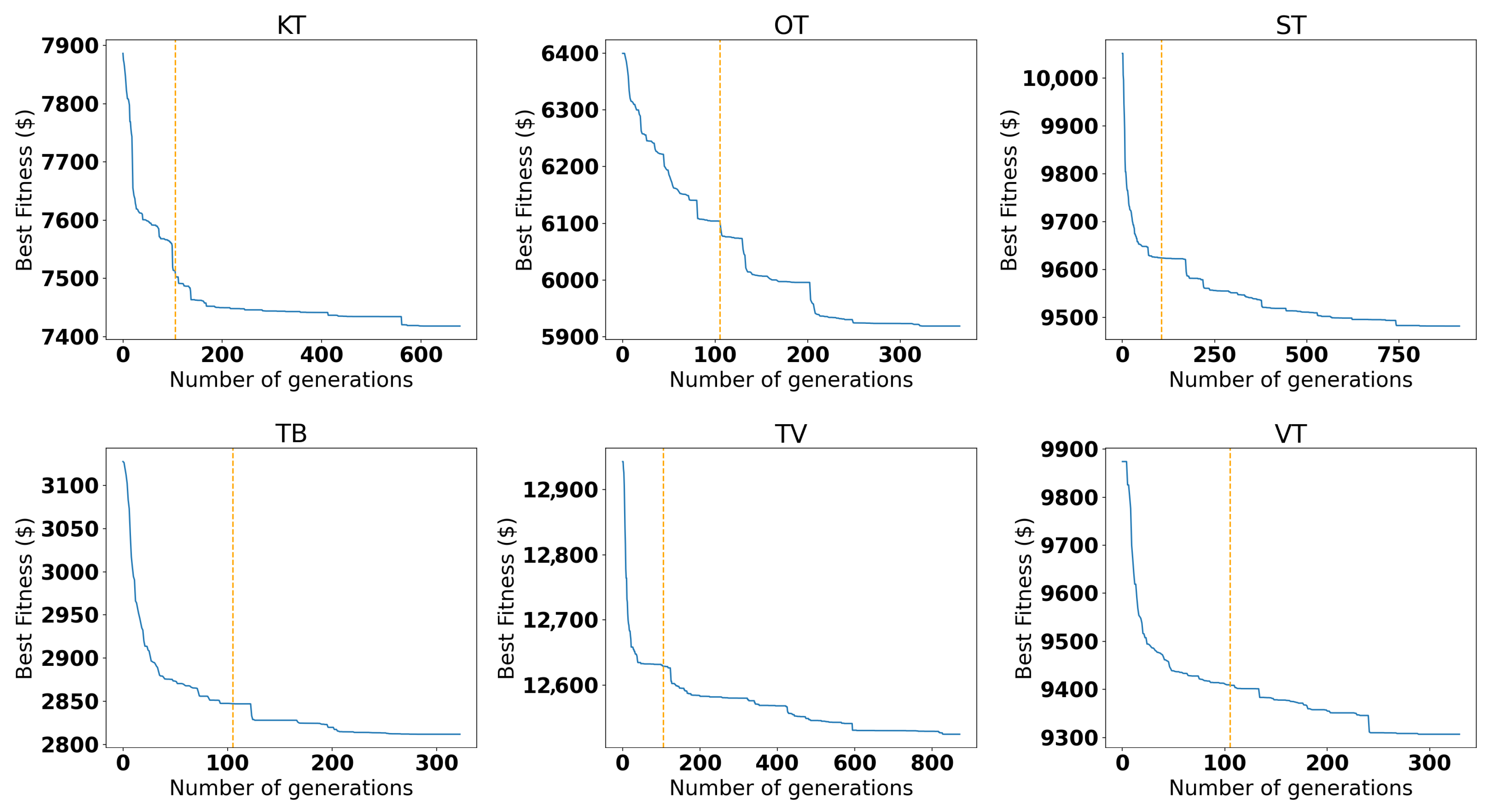
Convergence plot of the GA-Warm-Start approach for each instance. The dashed orange line represents the best solution obtained at the generation limit (15,000 individuals, which represents 105 generations).
Figure 10.
Convergence plot of the GA-Warm-Start approach for each instance. The dashed orange line represents the best solution obtained at the generation limit (15,000 individuals, which represents 105 generations).
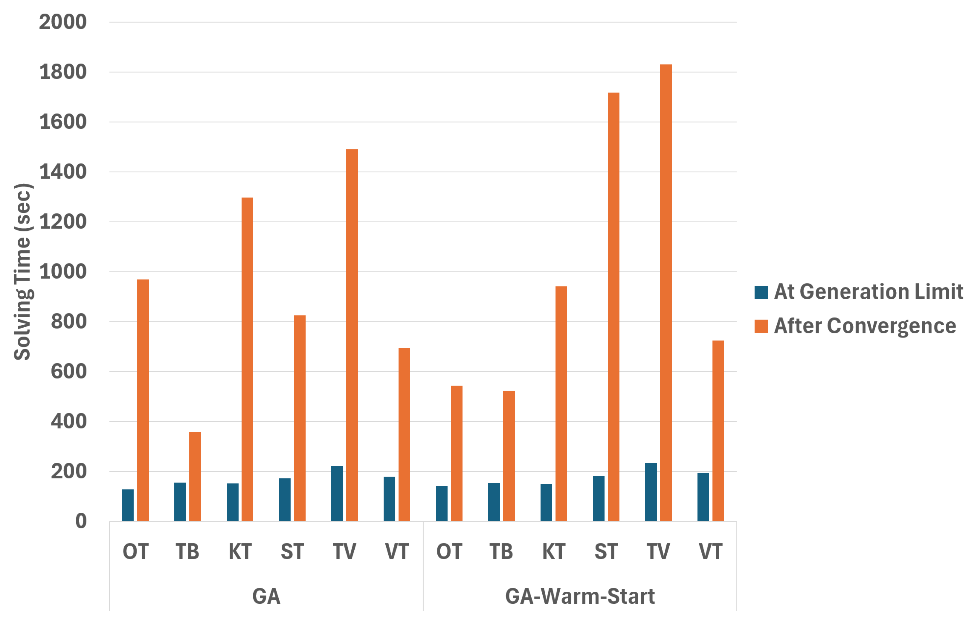
Figure 11.
Solving time (s) of the genetic algorithms with and without warm start for each instance at generation limit (15,000 individuals) and after convergence (40 consecutive generations without improvements).
Figure 11.
Solving time (s) of the genetic algorithms with and without warm start for each instance at generation limit (15,000 individuals) and after convergence (40 consecutive generations without improvements).
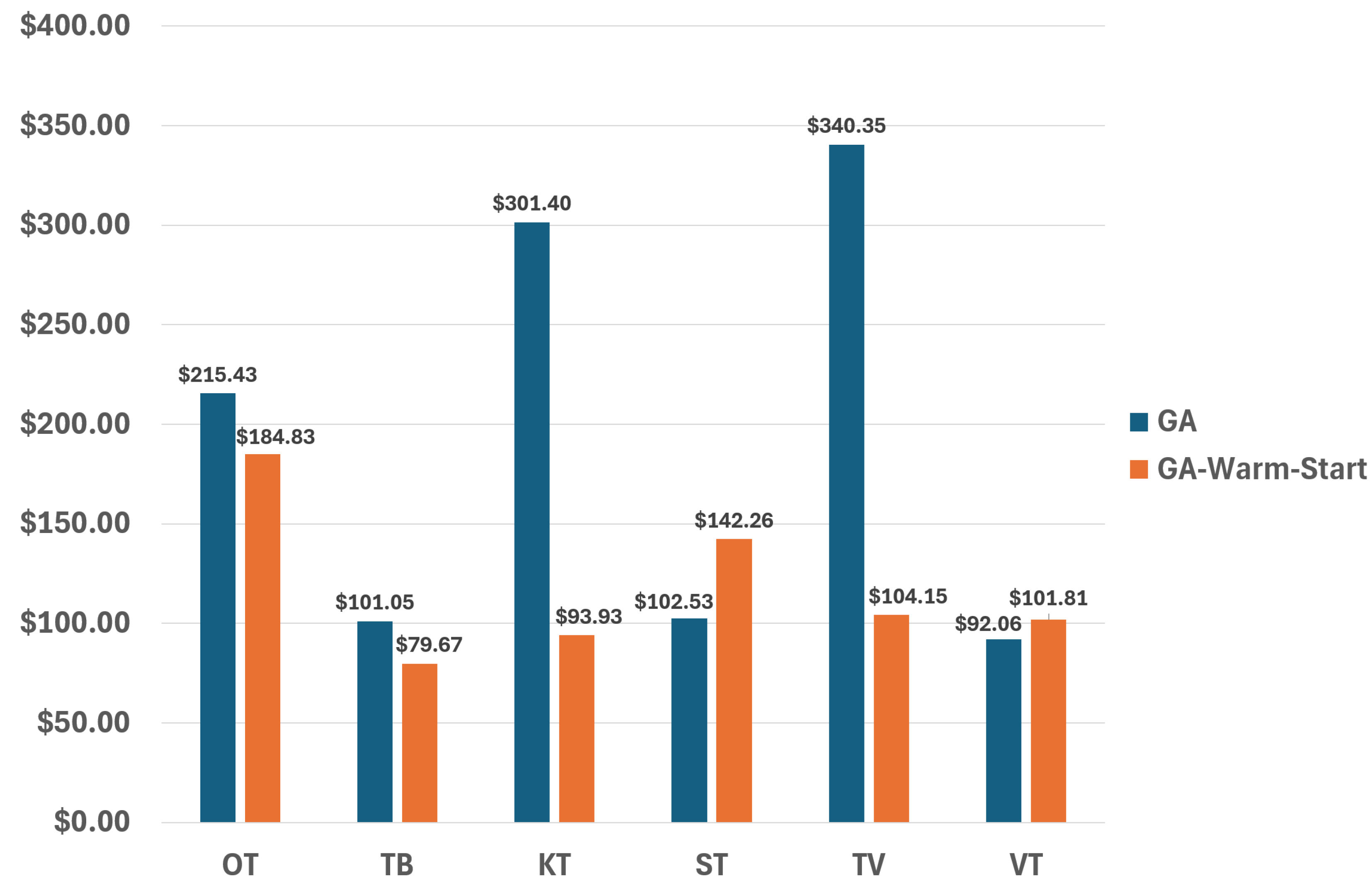
Figure 12.
Difference in total costs between the solution of each genetic algorithm between the solution obtained after convergence (40 consecutive generations without improvements) and the solution obtained at generation limit (15,000 individuals) for each instance.
Figure 12.
Difference in total costs between the solution of each genetic algorithm between the solution obtained after convergence (40 consecutive generations without improvements) and the solution obtained at generation limit (15,000 individuals) for each instance.
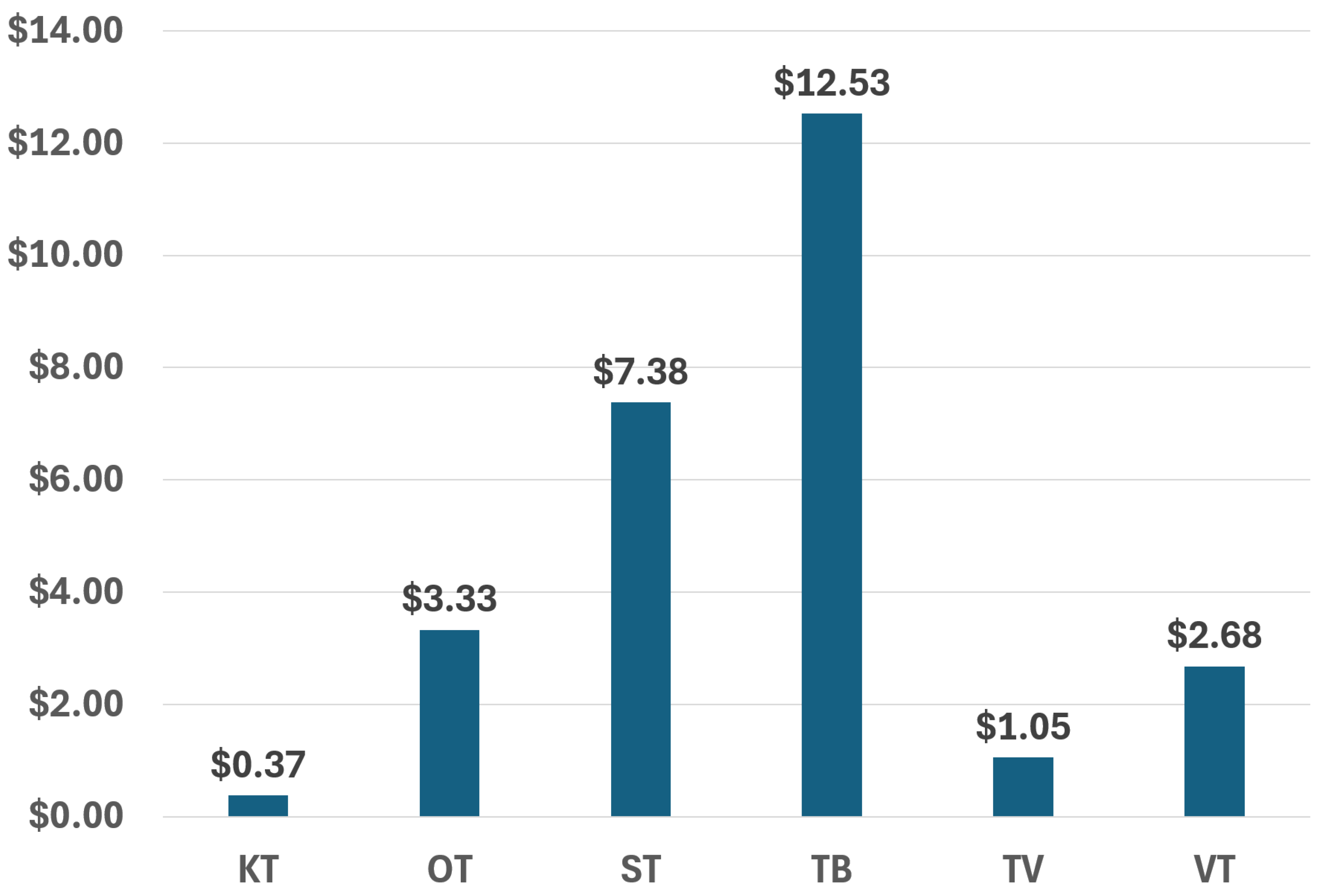
Figure 13.
Difference in total costs between the solution of the genetic algorithm that uses MIP solutions as warm start and the solution obtained by ITS-MIP-H for each instance.
Figure 13.
Difference in total costs between the solution of the genetic algorithm that uses MIP solutions as warm start and the solution obtained by ITS-MIP-H for each instance.
Table 1.
Description of the different parameters required by an instance of the S-FRHACP-VS, with their unit, split between the specific parameters for the FRHACP, the S-FRHACP, and the S-FRHACP-VS.
Table 1.
Description of the different parameters required by an instance of the S-FRHACP-VS, with their unit, split between the specific parameters for the FRHACP, the S-FRHACP, and the S-FRHACP-VS.
| Parameter | Description | Unit |
|---|
| FRHACP |
| Initial state of charge at the origin | % |
| Initial fuel quantity at the origin | L |
| Initial time at the origin | h |
| Minimal state of charge | % |
| Maximal state of charge | % |
| Minimal fuel quantity | L |
| Maximal fuel quantity | L |
| Scheduled departure time at terminal | h |
| Refueling rate of the aircraft | L/h |
| Fuel mass | kg/L |
| Empty aircraft mass | kg |
| Payload mass on leg | kg |
| Travel distance on leg | km |
| Recommended aircraft speed on leg | km/h |
| Function of the electricity consumption given the distance d (km), the mass m (kg), and the speed v (km/h) on leg | % |
| Function of the fuel consumption given the distance d (km), the mass m (kg), and the speed v (km/h) on leg | L |
| Electricity cost at terminal | CAD/% |
| Fuel cost at terminal | CAD/L |
| S-FRHACP |
| Scheduled arrival time at terminal | h |
| Minimal waiting duration at terminal | h |
| Maximal charging duration at terminal | h |
| Available fuel quantity at terminal | L |
| 1 if we can charge at terminal , else 0 | Bool |
| 1 if we can refuel at terminal , else 0 | Bool |
| 1 if we can use electricity on leg , else 0 | Bool |
| 1 if we can use fuel on leg , else 0 | Bool |
| Cost of arriving earlier than the scheduled arrival time at terminal | CAD/h |
| Cost of arriving later than the scheduled arrival time at terminal | CAD/h |
| Cost of departing earlier than the scheduled departure time at terminal | CAD/h |
| Cost of departing later than the scheduled departure time at terminal | CAD/h |
| S-FRHACP-VS |
| Minimal speed on leg | km/h |
| Maximal speed on leg | km/h |
Table 2.
Decision variables of the S-FRHACP-VS, with their domain and unit, split between the specific variables for the FRHACP, the S-FRHACP, and the S-FRHACP-VS.
Table 2.
Decision variables of the S-FRHACP-VS, with their domain and unit, split between the specific variables for the FRHACP, the S-FRHACP, and the S-FRHACP-VS.
| Variable | Domain | Description | Unit |
|---|
| FRHACP |
| | Arrival state of charge at node | % |
| | Departure state of charge at node | % |
| | Arrival fuel quantity at node | L |
| | Departure fuel quantity at node | L |
| | Traveled distance using electricity on leg | km |
| | Traveled distance using fuel on leg | km |
| S-FRHACP |
| | Waiting duration at terminal | h |
| S-FRHACP-VS |
| | Aircraft speed using electricity on leg | km/h |
| | Aircraft speed using fuel on leg | km/h |
Table 3.
Variables of the Stage 2 MIP model and their initial domain.
Table 3.
Variables of the Stage 2 MIP model and their initial domain.
| Variable | Domain | Description | Unit |
|---|
| | Charging duration at terminal | h |
| | Refueling duration at terminal | h |
| | Waiting duration at terminal | h |
| | Arrival state of charge at node | % |
| | Departure state of charge at node | % |
| | Arrival fuel quantity at node | L |
| | Departure fuel quantity at node | L |
| | Mass of the aircraft when using electricity on leg | kg |
| | Mass of the aircraft when using fuel on leg | kg |
| | Traveled duration using electricity on leg | h |
| | Traveled duration using fuel on leg | h |
| | Arrival time at node | h |
| | Departure time at node | h |
| | Total cost for arriving early at terminal | CAD |
| | Total cost for arriving late at terminal | CAD |
| | Total cost for departing early at terminal | CAD |
| | Total cost for departing late at terminal | CAD |
Table 4.
Description of the ten instances forming the dataset including the number of terminal (), the number of waypoints (), the total duration and distance of the combined flights, the electricity cost range (), and the fuel cost range () of each instance.
Table 4.
Description of the ten instances forming the dataset including the number of terminal (), the number of waypoints (), the total duration and distance of the combined flights, the electricity cost range (), and the fuel cost range () of each instance.
| Instance | | | Duration | Distance (km) | (CAD/kWh) | (CAD/L) |
|---|
| PN | 4 | 59 | 4 h 30 min | 2740 | 0.1397 | 1.46 |
| TB | 5 | 42 | 6 h 42 min | 2812 | 0.1397 | 1.46 |
| MS | 6 | 30 | 7 h 22 min | 2294 | 0.0533 | [1.16, 1.25] |
| OT | 7 | 43 | 9 h 34 min | 4709 | [0.0533, 0.1140] | [1.03, 1.28] |
| KT | 7 | 47 | 10 h 45 min | 5165 | [0.0776, 0.1408] | [1.13, 1.38] |
| ST | 6 | 52 | 13 h 10 min | 6788 | [0.0898, 0.1234] | [1.03, 1.37] |
| TV | 6 | 64 | 14 h 36 min | 8493 | [0.0976, 0.1408] | [1.13, 1.44] |
| SK | 7 | 107 | 16 h 33 min | 9456 | [0.0533, 0.1408] | [1.16, 1.44] |
| BK | 10 | 72 | 16 h 46 min | 8143 | [0.0590, 0.1408] | [1.13, 1.44] |
| VT | 5 | 49 | 11 h 17 min | 5886 | [0.0776, 0.1408] | [1.26, 1.41] |
Table 5.
Solving time of each instance in seconds as well as total costs—distinguished between the minimum, maximum, and mean costs over 20 runs with a confidence interval of 95% for the genetic algorithms (GA and GA-Warm-Start). Results reported for the Iterative Two-Stage MIP Heuristic (ITS-MIP-H); the ITS-MIP-H ran for a single iteration (ITS-MIP-H-One-It), the Stage 1 MIP model (S1-MIP-H), the genetic algorithms (GA and GA-Warm-Start), the dynamic programming approaches with and without the gradient descent post-treatment (DP and DP+GD), the Fuel-First Heuristic (FF-H), and the Max-Battery Heuristic (MB-H). The best results are in bold for each instance.
| Instance | Approach | Solving Time (s) | Total Costs (CAD) |
|---|
| Mean | Min | Max |
|---|
| TB | ITS-MIP-H | 8.47 ± 2.26 | 4053.79
|
| ITS-MIP-H-One-It | 2.8 ± 0.67 | 4273.82 |
| S1-MIP-H | 1.77 ± 0.37 | 4638.25 |
| GA-Warm-Start | 192.08 ± 33.47 | 4273.76 ± 54.25 | 4221.96 | 4343.96 |
| GA | 190.0 ± 32.02 | 4571.74 ± 460.19 | 4232.65 | 5036.84 |
| DP+GD | 1.35 ± 0.45 | 4691.55 |
| DP | 1.35 ± 0.45 | 4691.55 |
| MB-H | 0.64 ± 0.45 | 5018.40 |
| FF-H | 0.07 ± 0.02 | 5050.80 |
| OT | ITS-MIP-H | 8.88 ± 2.61 | 5698.82 |
| ITS-MIP-H-One-It | 3.5 ± 0.91 | 6037.98 |
| S1-MIP-H | 1.75 ± 0.45 | 6380.47 |
| GA-Warm-Start | 178.84 ± 29.56 | 6069.29 ± 160.81 | 5925.75 | 6223.41 |
| GA | 172.84 ± 29.59 | 6351.04 ± 313.95 | 6090.42 | 6593.51 |
| DP+GD | 4.7 ± 1.86 | 6399.29 |
| DP | 1.44 ± 0.51 | 6675.27 |
| MB-H | 0.78 ± 0.3 | 7471.08 |
| FF-H | 0.08 ± 0.04 | 7925.38 |
| KT | ITS-MIP-H | 17.85 ± 4.32 | 7257.39 |
| ITS-MIP-H-One-It | 6.13 ± 1.22 | 7276.22 |
| S1-MIP-H | 4.36 ± 1.13 | 7760.52 |
| GA-Warm-Start | 205.04 ± 33.27 | 7562.22 ± 90.32 | 7491.41 | 7652.06 |
| GA | 197.59 ± 33.63 | 7753.63 ± 196.47 | 7516.39 | 7867.23 |
| DP+GD | 4.66 ± 1.38 | 7886.30 |
| DP | 1.62 ± 0.74 | 8085.75 |
| MB-H | 1.27 ± 0.81 | 8454.27 |
| FF-H | 0.1 ± 0.06 | 9082.64 |
| ST | ITS-MIP-H | 13.59 ± 3.36 | 9464.36 |
| ITS-MIP-H-One-It | 8.71 ± 2.24 | 9464.36 |
| S1-MIP-H | 2.36 ± 0.71 | 9943.74 |
| GA-Warm-Start | 254.99 ± 40.33 | 9626.34 ± 78.14 | 9532.82 | 9694.56 |
| GA | 249.36 ± 41.44 | 9737.01 ± 246.42 | 9584.15 | 9999.04 |
| DP+GD | 3.37 ± 0.92 | 10051.21 |
| DP | 1.74 ± 0.67 | 10,609.48 |
| MB-H | 1.86 ± 0.81 | 10,844.11 |
| FF-H | 0.1 ± 0.03 | 11,184.57 |
| TV | ITS-MIP-H | 19.24 ± 4.51 | 12,264.88 |
| ITS-MIP-H-One-It | 7.03 ± 1.62 | 12,386.53 |
| S1-MIP-H | 3.1 ± 0.63 | 12,882.24 |
| GA-Warm-Start | 322.62 ± 53.64 | 12,605.92 ± 42.12 | 12,583.10 | 12,654.47 |
| GA | 315.12 ± 47.48 | 12,874.55 ± 199.33 | 12,708.59 | 13,024.28 |
| DP+GD | 3.37 ± 1.1 | 12,943.05 |
| DP | 2.44 ± 1.15 | 13,111.35 |
| MB-H | 2.97 ± 1.01 | 13,449.69 |
| FF-H | 0.16 ± 0.11 | 13,931.27 |
| VT | ITS-MIP-H | 12.29 ± 3.25 | 8770.51 |
| ITS-MIP-H-One-It | 4.08 ± 1.21 | 8945.93 |
| S1-MIP-H | 1.55 ± 0.67 | 9371.25 |
| GA-Warm-Start | 250.4 ± 30.76 | 9407.06 ± 119.86 | 9294.66 | 9544.14 |
| GA | 241.74 ± 20.87 | 9295.94 ± 416.15 | 8909.14 | 9666.08 |
| DP+GD | 4.06 ± 1.64 | 9874.05 |
| DP | 1.59 ± 0.41 | 10,063.71 |
| MB-H | 1.56 ± 0.78 | 10,268.48 |
| FF-H | 0.08 ± 0.03 | 10,511.44 |
Table 6.
Comparison of ITS-MIP-H vs. genetic algorithm for different criteria, mainly the total costs, solving time, ease of implementation, and the need for function approximation.
Table 6.
Comparison of ITS-MIP-H vs. genetic algorithm for different criteria, mainly the total costs, solving time, ease of implementation, and the need for function approximation.
| Criterion | ITS-MIP-H | GA (Warm Start) | Remarks |
|---|
| Total Costs | Best overall | Slightly higher costs | GA still competitive (avg + CAD 321) |
| Solving Time | 13 s | 230–320 s | GA slower by 18–25× |
| Ease of Implementation | Complex (MIP, function linearization) | Simple (known frameworks) | GA is user-friendly and flexible |
| Function Approximation | Required (grid sampling approximations) | Not needed | GA supports black-box modeling |
