Article

Multi-Lane Congestion Control Model for Intelligent Connected Vehicles Integrating Optimal Traffic Flow Difference Information in V2X Environment

1
Practical Teaching Center, Guizhou University of Commerce, Guiyang 550014, China
2
Guizhou Provincial Engineering Research Center for Collaborative Intelligent Perception of Mountain Spatial Information, Guizhou University of Commerce, Guiyang 550014, China
3
School of Computer and Information Engineering, Guizhou University of Commerce, Guiyang 550014, China
*
Author to whom correspondence should be addressed.
World Electr. Veh. J. 2025, 16(8), 457; https://doi.org/10.3390/wevj16080457
Submission received: 13 June 2025 / Revised: 30 July 2025 / Accepted: 7 August 2025 / Published: 11 August 2025

Abstract

In the V2X environment, intelligent connected vehicles can obtain multi-dimensional traffic flow data in real time through the vehicle–road collaborative cyber–physical fusion system. Based on this, this study proposes a multi-lane traffic flow lattice model integrating optimal traffic flow difference estimation information to effectively suppress traffic congestion. The linear stability criterion of the system is derived through linear stability analysis, proving that the optimal traffic flow difference estimation can significantly expand the stable region and suppress traffic fluctuations caused by small disturbances. Furthermore, the perturbation method is used to derive the mKdV equation near the critical stability point of the system, revealing the nonlinear characteristics of traffic congestion propagating in the form of kink solitary waves, and indicating that the new consideration effect can effectively slow down the congestion propagation speed by adjusting the parameters of solitary waves (such as wave speed and amplitude). The numerical simulation results show that compared to the traditional model, the improved model exhibits enhanced traffic flow stability and robustness. Meanwhile, it reveals the nonlinear relationship between the increase of the number of lanes and the alleviation of congestion, and there is an optimal lane configuration threshold. The research results not only provide theoretical support for the optimization of traffic flow efficiency in intelligent transportation systems, but also provide a decision-making basis for dynamic lane management strategies in the V2X environment.

1. Introduction

The number of automobiles has rapidly increased over the past few decades. As a result, traffic congestion has become a prominent issue, attracting extensive attention from scholars. To better understand the formation and evolution of traffic congestion, numerous traffic flow models have been proposed. Based on the modeling scale, the constructed models can be roughly categorized into two types: microscopic models and macroscopic models. Microscopic traffic flow models focus on individual vehicle behavior, primarily investigated through car-following models [1,2] and cellular automata models [3,4]. Macroscopic traffic flow models focus on the collective behavior of traffic flow. These models are mainly described through continuum models [5,6] and lattice hydrodynamic models [7,8].
In 1998, Nagatani [7] combined the advantages of microscopic and macroscopic models to propose a lattice hydrodynamic model for single-lane traffic flow. This model allows for easy analysis of the density wave equation describing traffic congestion evolution, as well as efficient simulation of collective traffic behavior. Later, Nagatani [8] extended the model to two-lane traffic by incorporating lane-changing behavior. Several extended traffic flow lattice models have since been proposed. These models incorporate various factors into the traffic system, including the driver’s predictive effect [9,10,11], traffic jerk effect [12], curved roads with passing scenarios [13,14], honking effect [15,16], and the backward-looking effect [17,18,19]. These models offer rich perspectives that enable us to better comprehend complex traffic congestion issues.
In recent years, the application of V2X (vehicle-to-everything) technology in the transportation field has attracted extensive attention. In 2025, Verma et al. [20] proposed a new lattice traffic flow model for the mixed traffic environment where connected vehicles (CVs) and human-driven vehicles (HDVs) coexist under the V2V environment by introducing the area occupancy effect in mixed traffic scenarios. In the same year, Dangi et al. [21] developed an improved car-following model based on the full velocity difference model, integrating factors such as drivers’ memory and overtaking behavior in the V2X environment. Additionally, Peng et al. [22] constructed a new two-lane lattice model by considering the effect of continuous historical evolution messages in V2X scenarios. Meanwhile, Mehta et al. [23] proposed a new lattice traffic flow model with V2X communication functionality, taking into account the impact of optimal velocity deviation and reaction time effect on traffic systems.
Lattice models have been extensively studied. However, most studies focus on single-lane and two-lane scenarios, with limited research on multi-lane systems, which are common in the real world. As shown in Figure 1 [24], V2X technology in multi-lane environments allows drivers to capture and process traffic flow data in real-time. This significantly enhances their situational awareness. As a result, V2X technology reduces information asymmetry between lanes through information interaction, narrows the differences in decision-making environments (e.g., perception range, collaboration efficiency) among vehicles in various lanes, and thereby provides technical support for symmetric lane-changing. Consequently, in multi-lane systems, lane-changing is not limited to adjacent lanes; it can also occur between non-adjacent lanes (referred to as cross-lane changing). Such lane-changing mechanisms are more complex and variable compared to those in single-lane or two-lane systems, and they exert a more significant impact on traffic flow. Recently, several researchers have initiated studies on multi-lane systems using traffic flow lattice models. For instance, Madaan and Sharma put forward a multi-lane lattice model that takes the influence of optimal current difference into consideration [25]. Later, in 2022, the two scholars further studied how delayed feedback control affects multi-lane systems [26]. In 2023, Zhai et al. developed a new multi-lane lattice hydrodynamic model that includes the passing effect [27]. Most recently, in 2025, Xiao et al. presented a new multi-lane lattice model with empirical lane-changing rates taken into account [28]. The results of these multi-lane lattice models all show that adding lane-changing behavior into multi-lane systems can effectively ease traffic jams and improve traffic flow. On the other hand, within the V2X environment, among the real-time traffic information accessible to vehicles, the discrepancy between the expected optimal flux and the actual flux—referred to as the optimal estimation of flux difference information (OEFDI)—has been proven to play a key role in the performance of traffic systems [29,30]. In practice, leveraging the real-time data interaction and perception capabilities of the V2X environment, and through real-time communication technologies between Road-Side Units (RSUs) and On-Board Units (OBUs) of intelligent connected vehicles, coupled with edge computing functionalities, drivers can access real-time interactive decision-making information such as OEFDI. This enables them to adjust vehicle states accordingly, thereby achieving an optimal driving condition. Although extensive research has been conducted on the OEFDI effect in single-lane and two-lane systems, its utilization in multi-lane framework remains relatively underexplored. The mechanisms by which OEFDI improves the multi-lane traffic stability remain unclear in the V2X environment. To fill this research gap, we construct a novel multi-lane lattice model integrating both the OEFDI effect and multi-lane features. Subsequently, we conduct thorough theoretical analyses and numerical simulations on the proposed model. The objective of this study is to clarify how the OEFDI influences multi-lane systems.
This paper is structured as follows: Section 2 introduces a new multi-lane lattice model that takes the OEFDI effect into account. Section 3 carries out linear stability analysis to obtain the criteria for maintaining traffic flow stability in multi-lane systems. Section 4 performs nonlinear analysis and deduces the mKdV density wave equation, aiming to gain a deeper understanding of traffic congestion. Section 5 provides numerical simulations to validate the theoretical conclusions drawn in Section 3 and Section 4. Lastly, Section 6 summarizes the key results of the study.

2. Models

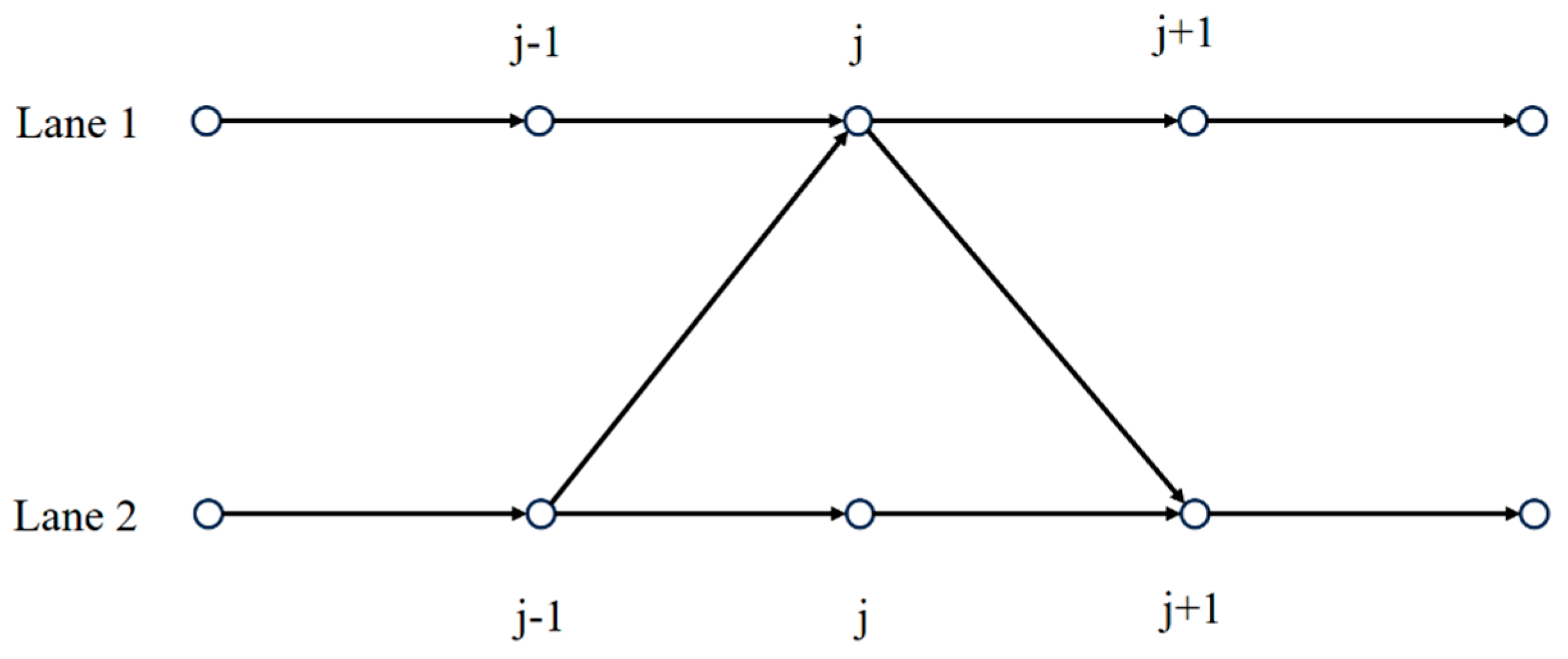
Before discussing the traffic flow behavior of multi-lane highways, we must briefly review the traffic flow modeling process for two-lane systems. In the two-lane scenario shown in Figure 2, both lanes are treated as uniform discrete grid points. Lane-changing occurs when traffic densities at the lattice sites on the two lanes differ. Lane-changing behavior aims to improve driving efficiency. If ρ 2 , j 1 ρ 1 , j > 0 holds, some traffic flow j 1 for lane 2 will shift to lane 1. This movement has a lane-changing rate of γ | ρ 0 2 V ( ρ 0 ) | ( ρ 2 , j 1 ρ 1 , j ) . Similarly, if ρ 1 , j ρ 2 , j + 1 > 0 , the lane-changing rate from j for lane 1 to j + 1 for lane 2 is γ | ρ 0 2 V ( ρ 0 ) | ( ρ 1 , j ρ 2 , j + 1 ) . The total change in lane-changing rate at lattice site j for lane 1 is determined as γ | ρ 0 2 V ( ρ 0 ) | ( ρ 2 , j 1 2 ρ 1 , j + ρ 2 , j + 1 ) . Therefore, the continuity equation (conservation equation) for lane 1 in the two-lane framework is obtained as follows [8]:
t ρ 1 , j ( t ) + ρ 0 ( ρ 1 , j ( t ) v 1 , j ( t ) ρ 1 , j 1 ( t ) v 1 , j 1 ( t ) ) = γ | ρ 0 2 V ( ρ 0 ) | ( ρ 2 , j 1 2 ρ 1 , j + ρ 2 , j + 1 )
Similarly, the conservation equation for lane 2 is given as follows:
t ρ 2 , j ( t ) + ρ 0 ( ρ 2 , j ( t ) v 2 , j ( t ) ρ 2 , j 1 ( t ) v 2 , j 1 ( t ) ) = γ | ρ 0 2 V ( ρ 0 ) | ( ρ 1 , j 1 2 ρ 2 , j + ρ 1 , j + 1 )
By adding Equations (1) and (2) together, it can be mapped to the following two-lane conservation equation,
t ρ j ( t ) + ρ 0 ρ j ( t ) v j ( t ) ρ j 1 ( t ) v j 1 ( t ) = γ ρ 0 2 V ρ 0 ρ j + 1 ( t ) 2 ρ j ( t ) + ρ j 1 ( t )
where ρ j = ( ρ 1 , j + ρ 2 , j ) / 2 , and ρ j v j = ( ρ 1 , j v 1 , j + ρ 2 , j v 2 , j ) / 2 . In a two-lane traffic system, ρ j ( t ) and v j ( t ) stand for the average density and speed of segment j at time t , respectively. The parameter ρ 0 refers to the overall average density of the entire traffic system, while the constant γ serves as the lane-changing coefficient that characterizes the intensity of lane-changing activities. The term | ρ 0 2 V ( ρ 0 ) | is introduced to render γ dimensionless. Furthermore, it is hypothesized that the longitudinal operation of the traffic flow is not associated with the lane-changing process, and the corresponding motion equation is presented below [8]:
ρ j ( t + τ ) v j ( t + τ ) = ρ 0 V ( ρ j + 1 ( t ) )
Here, V ( ρ ) is referred to as the optimized velocity function, which is a function of the density variable, and its formula is as follows [8]:
V ( ρ j ) = tanh ( 2 ρ 0 ρ j ( t ) ρ 0 2 1 ρ c ) + tanh ( 1 ρ c )
Here, ρ c represents the critical density. At ρ 0 = ρ c , the optimized velocity function V ( ρ ) has an inflection point at ρ j = ρ c .
Most past studies on traffic flow lattice modeling have focused on single-lane and two-lane systems. The operational principles of systems with more than two lanes have been less explored. In 2021, Madaan and Sharma [25] developed a new lattice model to better simulate the diffusion effect of lane-changing on traffic dynamics in multi-lane systems. This model, called the MS multi-lane lattice model, is designed for freeway systems with n lanes. In the MS multi-lane lattice model, all lanes are considered equivalent. Lane-changing can occur between any lanes, with the same probability for each lane. Meanwhile, in constructing the model, drivers’ individual differences are not considered. Instead, all drivers are assumed to have the same behavioral characteristics, driving habits, and response patterns. Additionally, Madaan and Sharma made the following assumptions when deriving the MS multi-lane lattice model [25]:
(1)
For 1 k n , the total number of vehicles in the k -th lane remains unchanged, and this conservation is only disrupted when lane-changing occurs.
(2)
The variable ρ k , j 1 represents the traffic density at position j 1 of the k -th lane. If ρ k , j 1 ρ m , j > 0 holds, where m ∈ [1, n] and m k , vehicles may change from k to lane m with lane-changing rate γ | ρ 0 2 V ( ρ 0 ) | ( ρ k , j 1 ρ m , j ) .
(3)
When ρ m , j ρ k , j + 1 > 0 holds, where m ∈ [1, n] and m k , vehicles are likely to change from lane m to lane k , with the lane-changing rate being γ | ρ 0 2 V ( ρ 0 ) | ( ρ m , j ρ k , j + 1 ) .
Based on these assumptions, the general continuity equation for the k -th lane in the MS multi-lane lattice model is as follows:
t ρ k , j + ρ 0 ( ρ k , j v k , j ρ k , j 1 v k , j 1 ) = γ | ρ 0 2 V ( ρ 0 ) | ( m = 1 m k n ρ m , j + 1 + m = 1 m k n ρ m , j 1 2 ( n 1 ) ρ k , j )
Here, ρ k , j and v k , j correspond to the traffic flow density and speed at site j of the k -th lane, respectively. The parameter n denotes the number of lanes in the multi-lane system.
For analysis, Madaan and Sharma rewrote Equation (6) as follows:
t ρ j + ρ 0 ( ρ j v j ρ j 1 v j 1 ) = γ ( n 1 ) | ρ 0 2 V ( ρ 0 ) | [ ρ j 1 + ρ j + 1 2 ρ j ]
where ρ j = 1 n k = 1 n ρ k , j , ρ j v j = 1 n k = 1 n ρ k , j v k , j .
The suppression of traffic congestion and the enhancement of traffic flow stability constitute the key components in modern traffic flow theory. The literature [29,30] shows that OEFDI information significantly improves stability in both single-lane and two-lane systems. However, studies addressing this factor within multi-lane scenarios remain fairly scarce. In particular, the effect of OEFDI information on traffic flow evolution during multi-lane lane-changing remains unclear. To address this gap, we introduce the OEFDI factor in a multi-lane context. We integrate it into the traffic flow motion Equation (4) as follows:
ρ j ( t + τ ) v j ( t + τ ) = ρ 0 V ( ρ j + 1 ) + k [ ρ 0 V ( ρ 0 ) ρ j v j ]
Here, Δ Q j = ρ 0 V ( ρ 0 ) ρ j v j represents the difference between expected optimal flux and current actual flux at site j at time t . The constant k is the corresponding response coefficient. By combining Equations (7) and (8), we create a new multi-lane lattice model that incorporates the OEFDI effect.
The core idea of the proposed model lies in the fact that, within multi-lane highway scenarios, drivers are able to acquire real-time traffic state information (including OEFDI) through V2X technology. Leveraging this information, they can promptly make decisions and modify the operational status of vehicles accordingly. After a mechanical and reaction delay time τ, these decisions influence the vehicle’s physical motion. This process drives the traffic state toward optimal flow. This process does not occur in isolation. It relies on coordinated lane-changing among drivers, optimizing traffic flow across the entire multi-lane system. Notably, when k = 0 and n = 2 , the proposed model simplifies to the Nagatini two-lane lattice model [8]. When n = 1, the model matches Yang’s model [29], and when n = 2 , it aligns with Peng’s model [30]. Thus, the models mentioned above are specific cases of the proposed model in this paper.
Eliminating the velocity variables from Equations (7) and (8) results in the following density evolution equation for the new model:
ρ j ( t + 2 τ ) ρ j ( t + τ ) + τ ρ 0 2 [ V ( ρ j + 1 ( t ) ) V ( ρ j ( t ) ) ] k { τ γ ( n 1 ) | ρ 0 2 V ( ρ 0 ) | [ ρ j + 1 ( t ) 2 ρ j ( t ) + ρ j 1 ( t ) ] ρ j ( t + τ ) + ρ j ( t ) } τ γ ( n 1 ) | ρ 0 2 V ( ρ 0 ) | [ ρ j + 1 ( t + τ ) 2 ρ j ( t + τ ) + ρ j 1 ( t + τ ) ] = 0
Formula (9) mainly depicts the recursive evolution relationship of the density variables ρ j 1 , ρ j , and ρ j + 1 at the three lattice positions of j 1 , j , and j + 1 at the times t + 2 τ , t + τ , and t . V and V′ correspond to the optimized speed function and its derivative, respectively.

3. Linear Stability Analysis

The steady-state solution for the new model is
v j ( t ) = V ( ρ 0 ) , v j ( t ) = V ( ρ 0 )
Let y j ( t ) be the small interference signal applied to lattice site j. At this time, the traffic density at site j deviates from the steady-state to become
ρ j ( t ) = ρ 0 + y j ( t )
Substituting Equation (10) into Equation (9) and then performing a linearization operation yields the following equation:
y j ( t + 2 τ ) y j ( t + τ ) + τ ρ 0 2 { V [ y j + 1 ( t ) y j ( t ) ] } k { τ γ ( n 1 ) ρ 0 2 V [ y j + 1 ( t ) 2 y j ( t ) + y j 1 ( t ) ] y j ( t + τ ) + y j ( t ) } τ γ ( n 1 ) ρ 0 2 V [ y j + 1 ( t + τ ) 2 y j ( t + τ ) + y j 1 ( t + τ ) ] = 0
Here, V ( ρ 0 ) = [ d V ( ρ j ) d ρ j ] | ρ j = ρ 0 . Expanding y j ( t ) in Equation (12) as a Fourier series form, y j ( t ) = exp ( i k j + z t ) , then setting the parameter z = z 1 i k + z 2 ( i k ) 2 + and substituting it into Equation (12), the first and second order terms for i k are obtained, respectively, after neglecting the higher order terms.
z 1 = 1 1 + k ρ o 2 V
z 2 = 3 + k 2 ( 1 + k ) z 1 2 τ 1 2 ( 1 + k ) ρ o 2 V + γ ( n 1 ) s
If z 2 is negative, the small perturbation signal will develop and amplify in the steady-state traffic, and the traffic flow in the multi-lane system will become unstable. However, if z 2 is positive, the small perturbation signal will be gradually weakened in the traffic flow with the development of time, and the multi-lane traffic flow will eventually converge to the steady state. The critical stability conditions of the system for the new model are thus obtained as follows:
τ c = ( 1 + k ) 2 [ 1 + 2 ( 1 + k ) ( n 1 ) γ ] ( 3 + k ) ρ o 2 V
Hence, the stabilization conditions for the new model are
τ < ( 1 + k ) 2 [ 1 + 2 ( 1 + k ) ( n 1 ) γ ] ( 3 + k ) ρ o 2 V
Specifically, for k = 0 , n = 2 , the stability condition (16) is consistent with Nagatini’s two-lane lattice model [8]. When n = 1 , the stability condition (16) is the same as that of Yang’s model [29]. As n = 2 , the stability condition (16) agrees well with the stability criterion of Peng’s model [30].
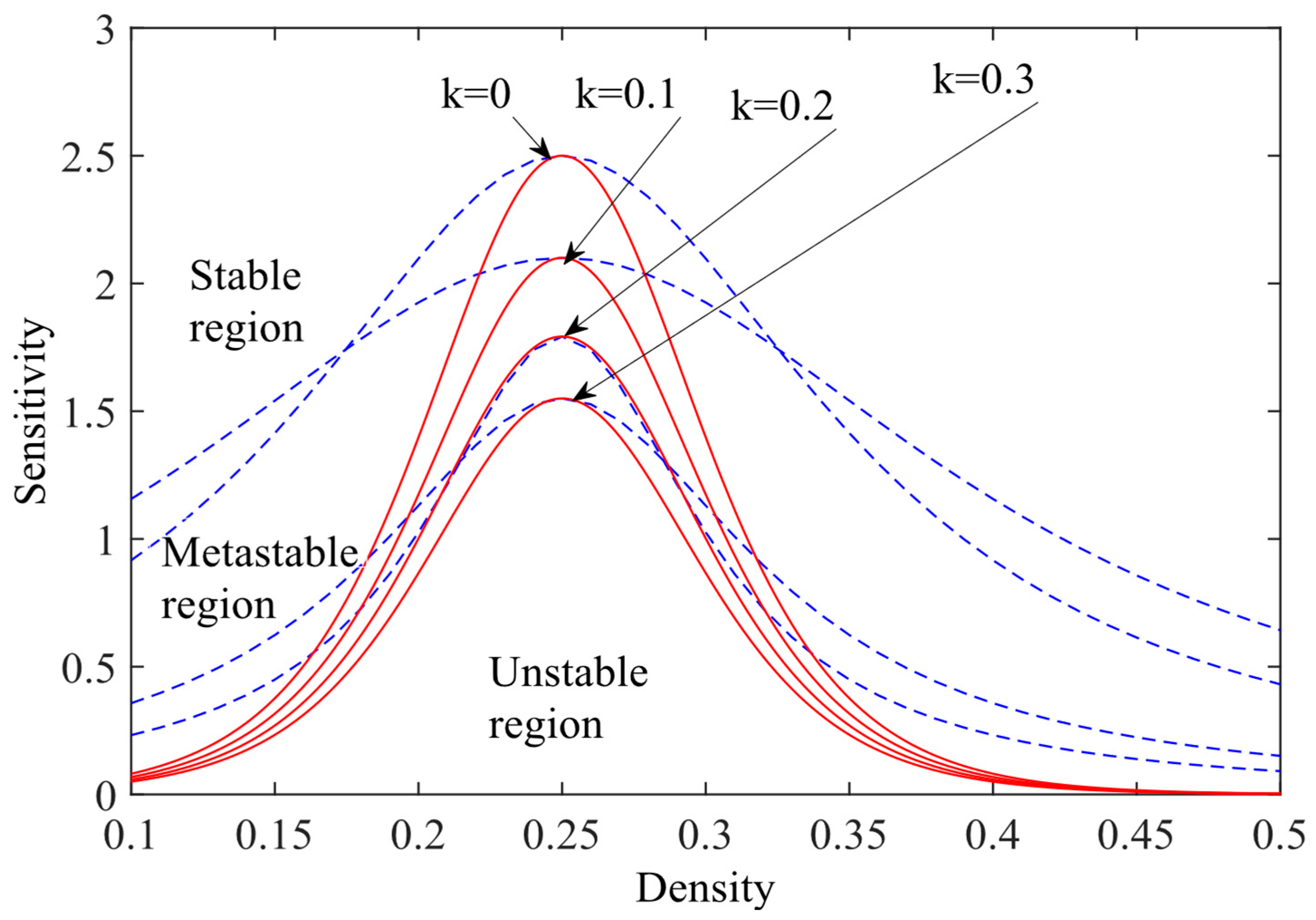
Figure 3 shows the phase diagram in parameter space ( ρ , a ) for the new model with different values of k when γ = 0.05 , n = 3. In Figure 3, solid lines represent the critical stability curves, while dashed lines show the coexistence curves (see Section 4 for details). The figure shows that each pair of critical stability and coexistence curves divide the phase space into three regions: stable, sub-stable, and unstable. When k = 0 the OEFDI factor is not considered, and the stability region of the traffic flow narrows. But when k 0 OEFDI information is included, it significantly enlarges the stable region in the multi-lane system. As the value of k increases, the critical stability and coexistence curves shift downward. This expansion of the stabilization region improves traffic flow stability in the multi-lane system. Clearly, OEFDI information has a significant positive effect on the macroscopic stability of multi-lane traffic.
Figure 4 illustrates the variation of the driver sensitivity coefficient with parameter k under different density conditions. It can be observed that within the interval [0, 0.5], the driver sensitivity is highly responsive to changes in k , decreasing rapidly as k increases—this indicates a significant improvement in traffic flow stability. However, when k > 0.5 , the rate of decrease in driver sensitivity slows down markedly, showing a gentle downward trend, which suggests that the marginal effect of k on traffic flow stability tends to diminish. However, it is important to emphasize that in practical applications, the reasonable value of parameter k should be calibrated by integrating the constraint range of stability conditions with field-measured data. Figure 5 shows the phase diagram for the proposed model with different lane numbers, where γ = 0.05 and k = 0.1. Figure 5 shows that traffic stability enhances as the lane count n rises. This suggests that the number of lanes plays a significant role in enhancing the stability of traffic flow in multi-lane systems.
Table 1 presents the critical sensitivity for our model (k = 0.1) and the MS multi-lane lattice model [25] (with β = 0 for comparable conditions) under varying lane numbers n. From Table 1, both models show critical sensitivity coefficients decreasing with more lanes, indicating improved traffic flow stability as lanes increase. However, our model consistently yields lower values than the MS model under the same lane count, demonstrating better stability.

4. Nonlinear Stability Analysis

To examine how traffic congestion evolves in the multi-lane highway system around the critical point ( ρ c , a c ) , slow variables X and T are defined in terms of spatial variable j and temporal variable t as follows:
X = ε ( j + b t ) , T = ε 3 t , 0 < ε 1
where parameter b is an undetermined quantity. Assume ρ j ( t ) satisfies the equation below:
ρ j ( t ) = ρ c + ε R ( X , T )
Plugging Equation (18) into Formula (9) and expanding via Taylor series up to ε5 gives the following equation:
ε 2 ( b + ρ c 2 V + k b ) X R + ε 3 [ 3 + k 2 b 2 τ + 1 + 2 γ ( n 1 ) ( 1 + k ) 2 ρ c 2 V ] X 2 R + ε 4 [ ( 1 + k ) T R + ( 7 + k 6 b 3 τ 2 + 1 6 ρ c 2 V + γ ( n 1 ) ρ c 2 V b τ ) X 3 R + 1 6 ρ c 2 V X R 3 ] + ε 5 { ( 3 + k ) b τ T X R + [ 15 + k 24 b 4 τ 3 + 1 24 ρ c 2 V + 1 2 γ ( n 1 ) ρ c 2 V ( b τ ) 2 + 1 + k 12 γ ( n 1 ) ρ c 2 V ] X 4 R + 1 12 ρ c 2 V X 2 R 3 } = 0
where V = [ d V ( ρ j ) d ρ j ] | ρ j = ρ c , V = [ d 3 V ( ρ j ) d ρ j 3 ] | ρ j = ρ c .
To eliminate the second and third order terms of ε in Equation (19), let τ = ( 1 + ε 2 ) τ c and b = 1 1 + k ρ c 2 V , then Equation (19) can be changed to
ε 4 [ T R g 1 X 3 R + g 2 X R 3 ] + ε 5 [ g 3 X 2 R + g 4 X 4 R + g 5 X 2 R 3 ] = 0
where g 1 = ( 7 + k ) b 3 τ c 2 + ρ c 2 V + 6 γ ( n 1 ) ρ c 2 V b τ c 6 ( 1 + k )
g 2 = ρ c 2 V 6 ( 1 + k ) ,
g 3 = 3 + k 2 ( 1 + k ) b 2 τ c ,
g 4 = 1 1 + k [ 15 + k 24 b 4 τ c 3 + 1 24 ρ c 2 V + 1 2 γ ( n 1 ) ρ c 2 V ( b τ c ) 2 + 1 + k 12 γ ( n 1 ) ρ c 2 V + ( 3 + k ) b τ c g 1 ] ,
g 5 = 1 1 + k [ 1 12 3 + k 6 ( 1 + k ) b τ c ] ρ c 2 V .
Introducing the subsequent mathematical transformation,
T = g 1 T ,   R = g 1 g 2 R
Equation (20) can be changed by adding correction terms o ( ε ) to create the mKdV equation.
T R X 3 R + X R 3 + ε M [ R ] = 0
where
M [ R ] = 1 g 1 [ g 3 X 2 R + g 4 X 4 R + g 1 g 5 g 2 X 2 R 3 ]
Ignoring the O ( ε ) term, the kink–antikink solution is given by
R 0 ( X , T ) = c tanh c 2 ( X c T )
The parameter c denotes the density wave speed, which is determined by the following solvability conditions:
( R 0 , M [ R 0 ] ) = + d X R 0 ( X , T ) M [ R 0 ( X , T ) ] = 0
In [32], the authors derive the specific calculation formula for c as follows:
c = 5 g 2 g 3 / ( 2 g 2 g 4 3 g 1 g 5 )
Hence, the kink–antikink density wave solution of the new model is given by the following formula:
ρ j ( t ) = ρ c + g 1 c g 2 ( τ τ c 1 ) tanh c 2 ( τ τ c 1 ) [ j + ( 1 c g 1 ( τ τ c 1 ) ) t ]
The corresponding amplitude A can be calculated using the formula
A = g 1 c g 2 ( τ τ c 1 )
The kink–antikink density wave solution in nonlinear analysis reveals the key characteristics of traffic blockage near the critical point. These features include a free-flow phase at low density and a blockage phase at high density. The coexistence curves illustrate the free-flow phase at low density and the traffic jam phase at high density. Figure 3 and Figure 4 show the coexistence curves. Figure 3 relates these curves to the response coefficients of the OEFDI effect, while Figure 4 links them to the lane count. The nonlinear analysis results also highlight the relationship between the number of lanes and the OEFDI parameters. These factors strongly influence the propagation speed and fluctuation amplitude of the kink–antikink density wave (traffic jam).

5. Numerical Simulation

5.1. Experimental Design

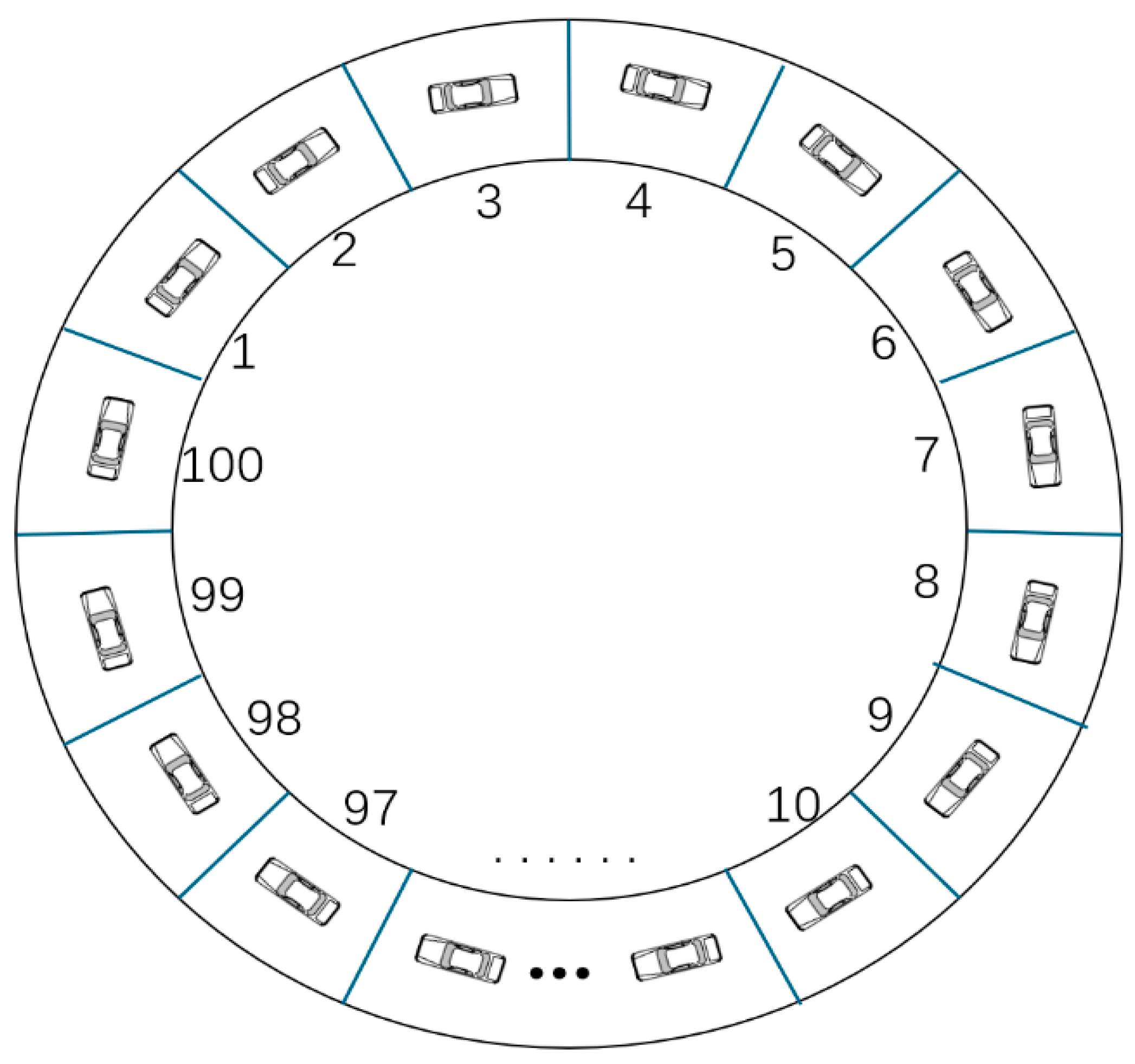
This section presents numerical simulations for the density evolution equation of the multi-lane traffic flow system, represented by Equation (9). The simulation adopts the periodic boundary conditions, as illustrated in Figure 6, where vehicles travel on a circular road with the end of the segment connected to its start. Specifically, when a vehicle reaches the end of the segment, it re-enters from the start; conversely, vehicles exiting from the start will enter from the end. Through this setup, the road segment is transformed into a boundary-free closed system, thereby eliminating the interference caused by vehicles entering or exiting at the boundaries. The initial states were set as follows:
ρ j ( 0 ) = ρ 0 = 0.25 ρ j ( 1 ) = ρ j ( 0 ) = ρ 0 : j 50 , 51 ρ j ( 1 ) = ρ 0 0.1 : j = 50 ρ j ( 1 ) = ρ 0 + 0.1 : j = 51
The input parameters for the simulation are N = 100 , γ = 0.05 , and ρ c = ρ 0 = 0.25 . For ease of reference, Table 2 extracts the main parameters of the new model. The results are shown in Figure 7, Figure 8, Figure 9 and Figure 10.

5.2. Results Analysis and Discussion

5.2.1. Analysis of the Density Wave Evolution
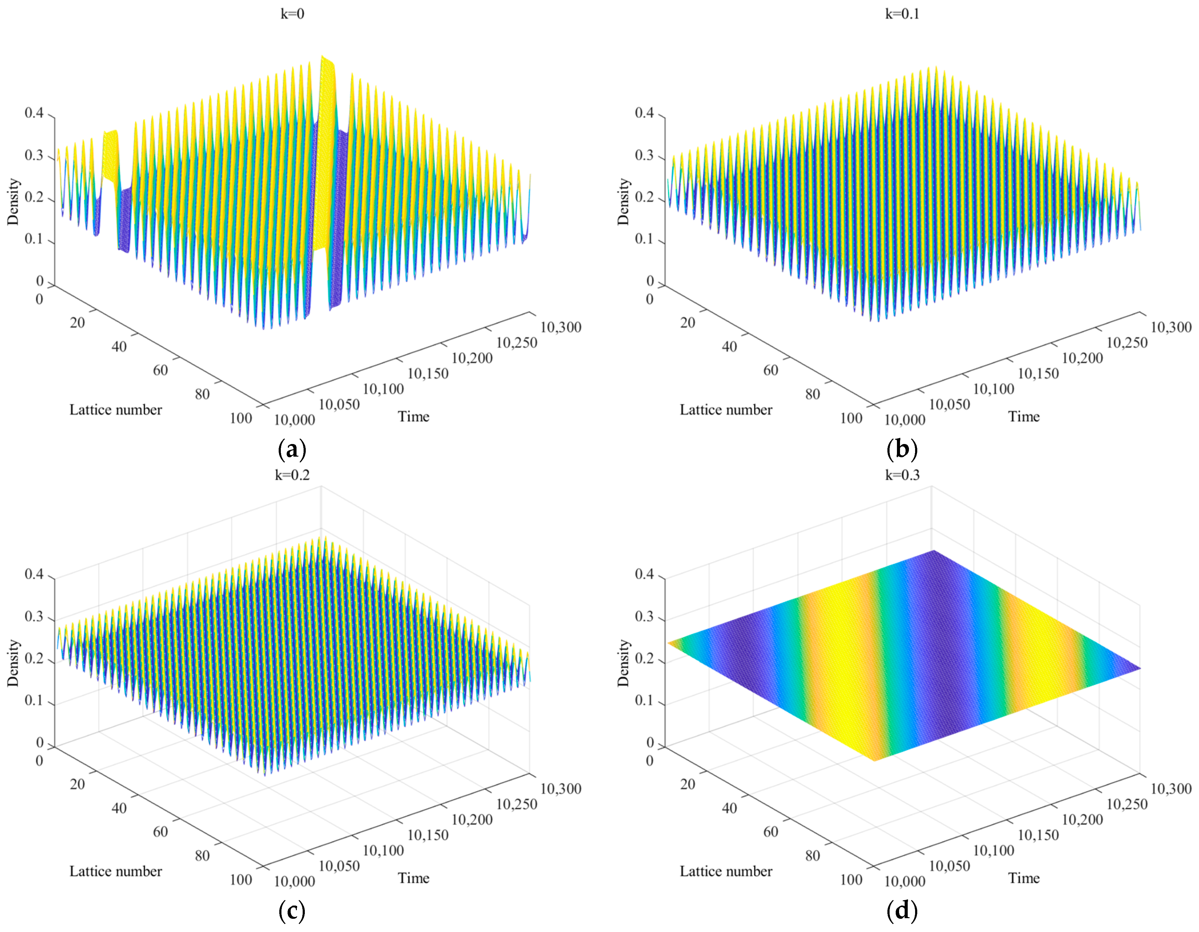
Figure 7a–d show the spatio-temporal distribution of traffic density after 10,000 time steps. To maintain consistency with the parameters of Yang’s model in Reference [29], we set k = 0 ,   0.1 ,   0.2 , and 0.3, and the remaining parameters are set as a = 1.7 and n = 3 . When k = 0 , corresponding to the pattern in Figure 7a, the OEFDI information is not considered. Over time, small perturbations in the traffic flow evolve into a stop-and-go traffic density wave, leading to congestion. When k 0 , meaning the OEFDI effect is considered, the amplitude of traffic congestion in Figure 7b–d decreases significantly compared to Figure 7a. As k increases, the fluctuation amplitude in Figure 7b–d gradually decays. This effectively alleviates traffic congestion. When k = 0.3 , the stability condition of Equation (15) is satisfied. At this point, small perturbations disappear over time, and the traffic flow returns to a balanced steady state.
To better illustrate the stabilizing effect of OEFDI information on the multi-lane highway system, Figure 8 complements Figure 5. It shows the relationship between the density difference, ρ j ( t )     ρ j ( t 1 ) , and the density, ρ j t , during the time interval t = 10,000–10,300. Figure 8 also displays the distribution of traffic density across all lattice sites at time step t = 10,300. Figure 8 reveals that as parameter k increases, the area of the closed hysteresis loop formed by the data pairs ( ρ j ( t )     ρ j ( t 1 ) ,   ρ j ( t ) ) becomes smaller. This results in a narrower range of traffic density fluctuations and a reduced amplitude of the corresponding kink–antikink density wave. These changes imply that traffic flow stability is effectively enhanced.
Figure 7. Space-time evolution of the density for (a) k = 0 , (b) k = 0.1 , (c) k = 0.2 , and (d) k = 0.3 , with a = 1.7 and n = 3 .
Wevj 16 00457 g007
Figure 8. The plots of density difference, ρ j (t) − ρ j (t − 1), against density, ρ j   (t), and the density profiles of the density wave at t = 10,300 for a = 1.7 and n = 3 . The plots are shown for (a) k = 0 , (b) k = 0.1, (c) k = 0.2, and (d) k = 0.3, respectively. The circles represent hysteresis loops. The smaller the area of a loop, the stronger the stability of the traffic flow.
Wevj 16 00457 g008
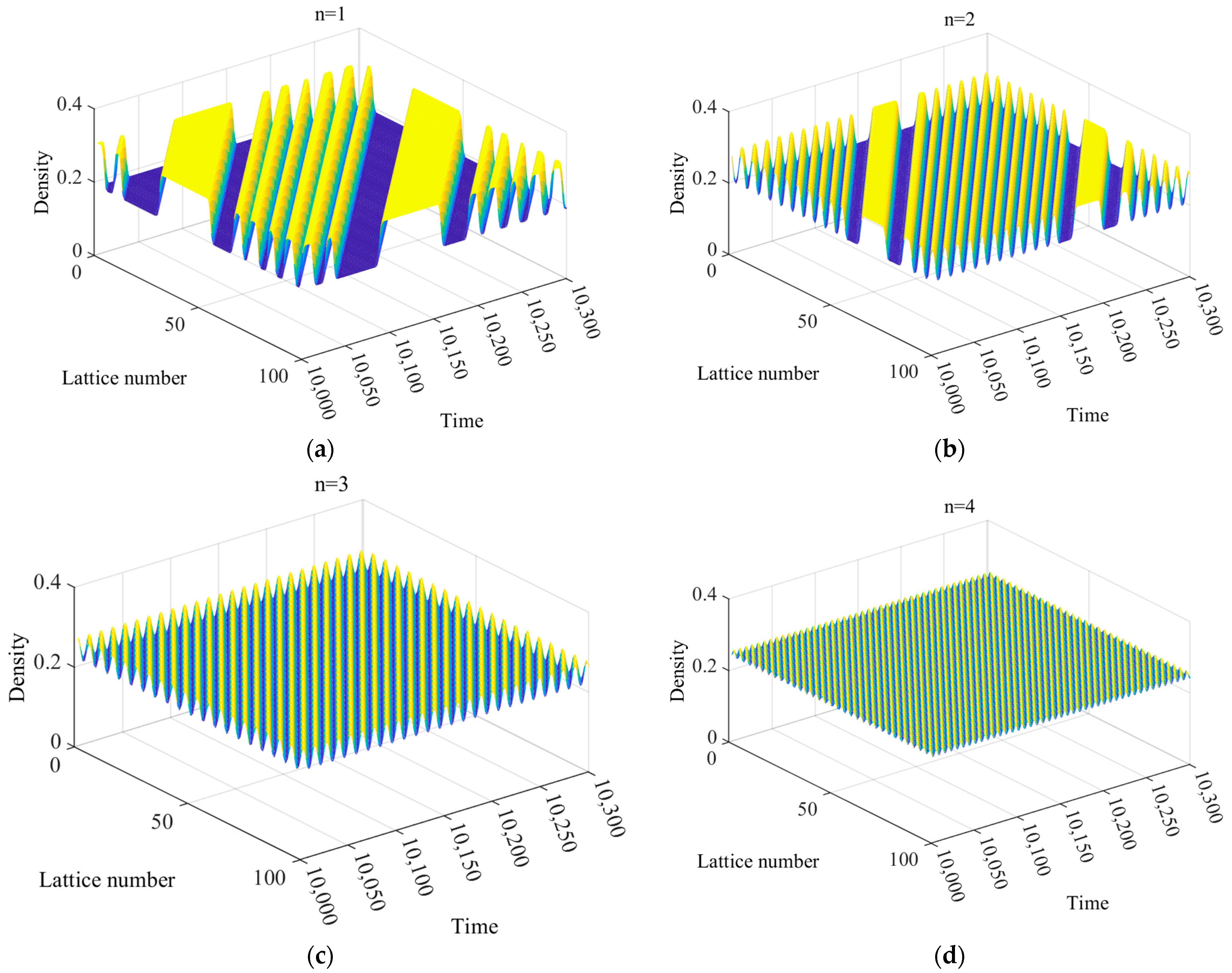
Figure 9a–d show the spatio-temporal distribution of traffic density in a multi-lane system after 10,000 time steps. In real-world traffic, the lane count in multi-lane systems typically ranges from one to four. Meanwhile, simulations of existing multi-lane system models [25,26,27,28] also commonly adopt this range (one to four lanes). Therefore, in the simulations of this paper, the number of lanes n is set to 1, 2, 3, and 4, respectively. The input parameters are a = 2 and k = 0.1 . For n = 1 , the density evolution pattern in Figure 9a matches Yang’s model [29]. For n = 2 , the density evolution pattern in Figure 9b matches Peng’s model [30]. Comparing Figure 9a,b, it is clear that lane-changing diffusion reduces traffic congestion in the two-lane system. The congestion in Figure 9b is significantly less than that in the single-lane system shown in Figure 9a. As the number of lanes increases to three and four, as shown in Figure 9c,d, the fluctuation amplitude between the free-flow phase and the blocking phase decreases further. The traffic density at each lattice site fluctuates slightly around the equilibrium density. As a result, the stability of the traffic flow is significantly enhanced.
Figure 9. Space-time evolution of the density for (a) n = 1 , (b) n = 2 , (c) n = 3 , and (d) n = 4 . ( a = 2 , k = 0.1 ).
Wevj 16 00457 g009
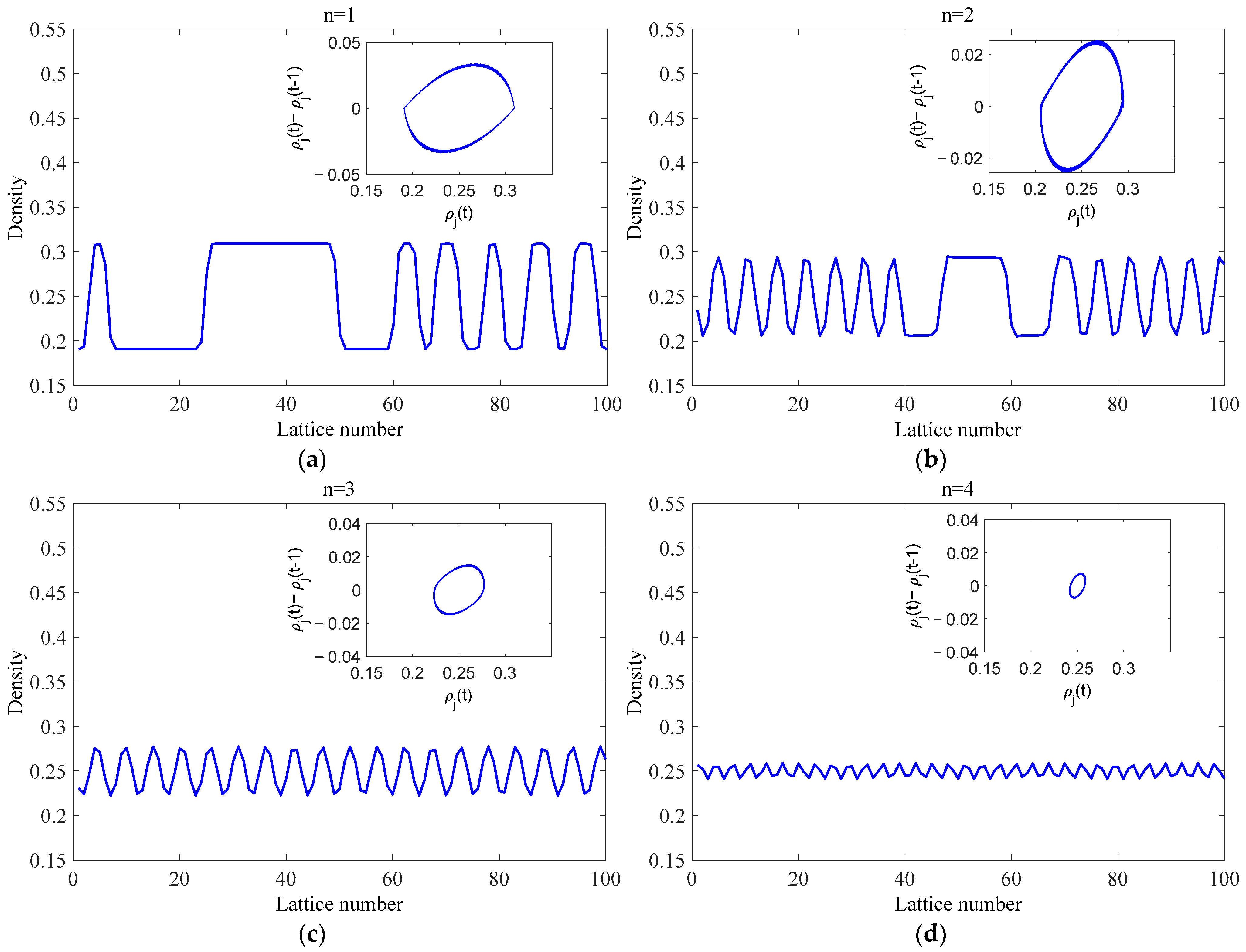
Figure 10 corresponds to Figure 9 and plots the density difference, ρ j ( t )     ρ j ( t 1 ) , versus the density, ρ j ( t ) , for different lane numbers n at times t = 10,000–10,300. It also shows the distribution of traffic density at all lattice sites at time step t = 10,300 . Figure 10 shows that as the number of lanes increases, the area of the hysteresis loop becomes smaller. The fluctuation amplitude of the kink–antikink density wave also decreases significantly. This indicates that a higher lane count leads to enhanced stability and anti-interference capability in the multi-lane system, resulting in smoother traffic flow.
The linear stability analysis results outlined in Section 3 receive validation from the simulation findings in Figure 7, Figure 8, Figure 9 and Figure 10. These results validate the importance of the OEFDI effect and the function of lane quantity in the efficient movement of traffic flow. Figure 8 and Figure 10 both show the kink–antikink density wave representing traffic congestion propagating upstream, as predicted by the nonlinear analysis. In Figure 8 and Figure 10, the increase of the response coefficients of the OEFDI effect and the number of lanes causes the amplitude of the kink–antikink density wave to gradually decrease. Overall, these findings lead to several important conclusions: Introducing OEFDI information into multi-lane highway systems effectively improves traffic flow stability by reducing the negative effects of external interference. Additionally, increasing the number of lanes positively impacts traffic flow stability.
Figure 10. Plots of density difference ρ j ( t ) ρ j ( t 1 ) against density ρ j ( t ) and the density profiles of the density wave at t =   10,300 when a = 2 , k = 0.1 for (a) n = 1 , (b) n = 2 , (c) n = 3 , and (d) n = 4 , respectively. The circles represent hysteresis loops. The smaller the area of a loop, the stronger the stability of the traffic flow.
Wevj 16 00457 g010

5.2.2. Analysis of Traffic Flow Optimization

Optimizing traffic efficiency is a critical topic. To investigate the OEFDI effect and the impact of lane quantity on traffic flow, the 25th road segment was selected as the observation point, from which traffic flow data were collected within the time interval t = 10,000 to 10,300. Statistical calculations were performed using these data to determine the average flow value of the system. The initial conditions were set as follows: ρ j ( 0 ) = ρ 0 = 0.25 , ρ j ( 1 ) = ρ j ( 0 ) = ρ 0 for j 50 ,   51 , ρ j ( 1 ) = max ( 0 , ρ 0 0.1 ) for j = 50 , and   ρ j ( 1 ) = ρ 0 + 0.1 for j = 51 . Figure 11 and Figure 12 present the simulation results.
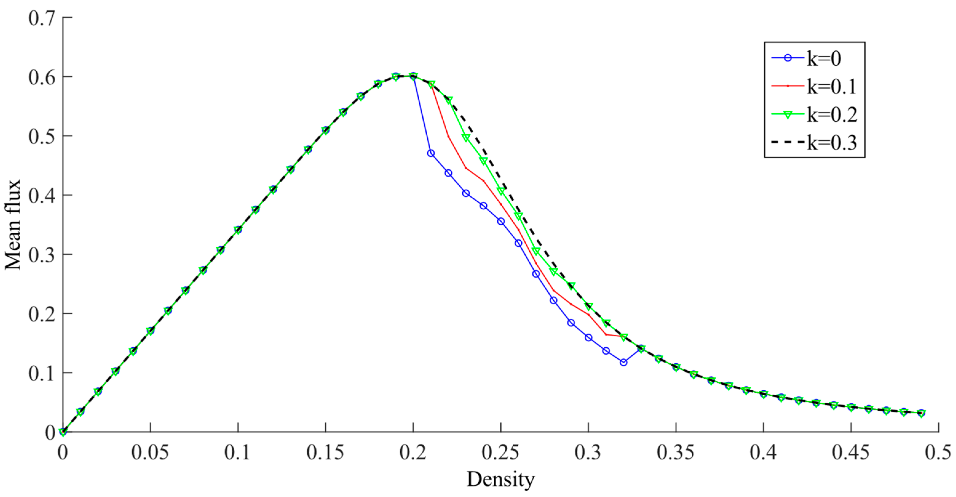
Figure 11 illustrates the relationship between initial density and average flow across varying k values in the new model. Figure 11 shows that OEFDI information has little effect on the multi-lane mean traffic flux in low-density ( ρ 0 < 0.20 ) and high-density ( ρ 0 > 0.33 ) regions. However, when the traffic density exceeds a certain threshold, OEFDI information becomes crucial. It significantly increases the multi-lane average flux. At this point, the flow rate with OEFDI is noticeably higher than when this factor is not considered. Additionally, the multi-lane average flux increases with the value of k.
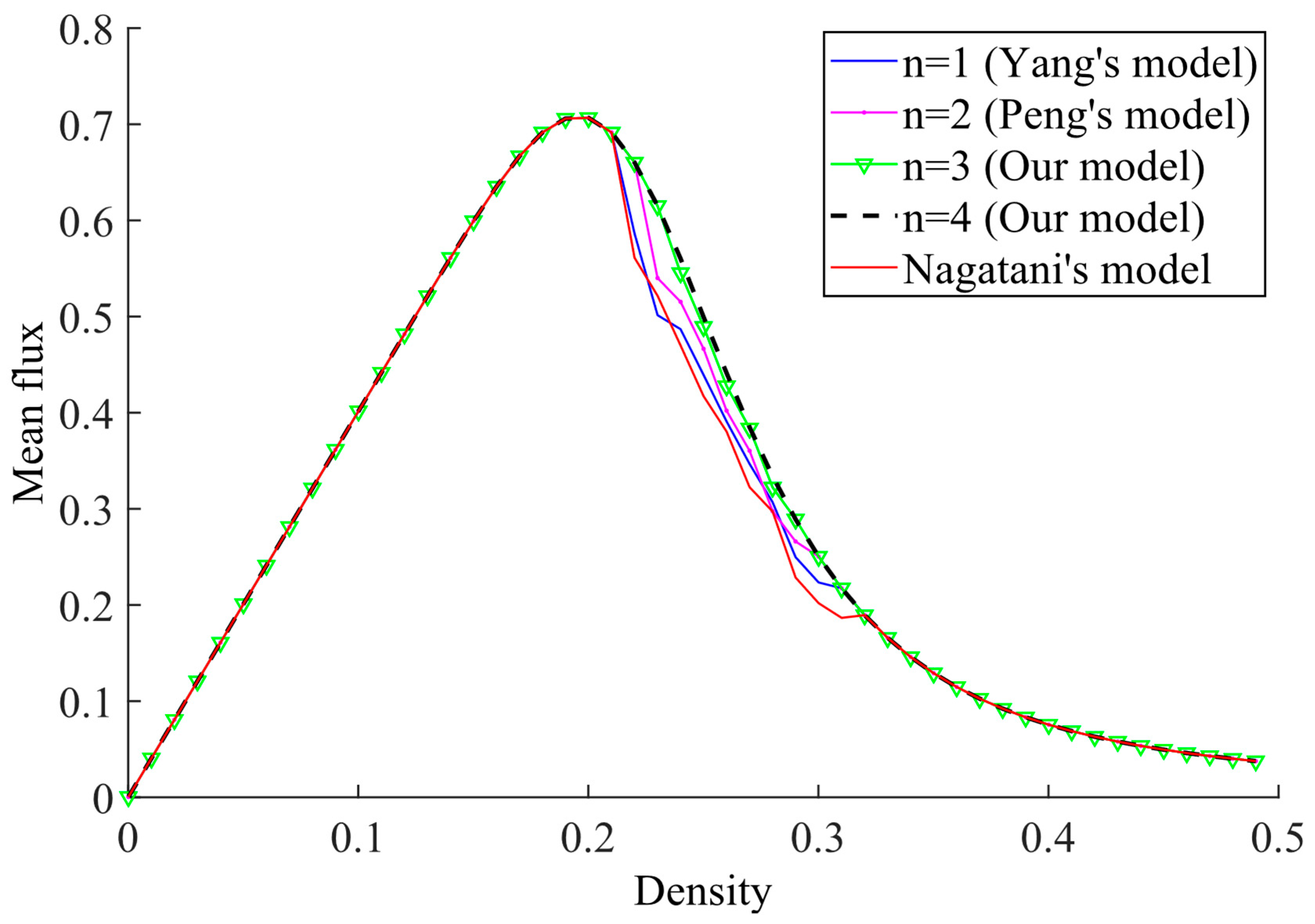
Figure 12 shows the relationship between the system’s mean flux and density. It covers various number of lanes. For the purpose of comparison, the flow curve corresponding to Nagatani’s model is also presented herein. Figure 12 shows that increasing the number of lanes has little impact on mean flux in the free-flow state at low density ( ρ 0 < 0.20 ). Similarly, it has no significant effect in the jam state at high density ( ρ 0 > 0.33 ). However, adding more lanes becomes important when vehicle density surpasses the critical point and enters a specific range ( 0.20 ρ 0 0.33 ). At this point, the average flux increases significantly with the addition of lanes. Traffic efficiency also improves as conditions for lane-changing become favorable. Meanwhile, within this density interval, the proposed model in this paper exhibits a higher flow level compared to Yang’s model, Peng’s model, and Nagatani’s model.
From the simulation results in Figure 11 and Figure 12, we can draw several conclusions. The introduction of OEFDI information in multi-lane systems greatly improves traffic flow. Similarly, increasing the number of lanes enhances traffic efficiency. Overall, OEFDI information plays a crucial role in the operation of traffic flow in multi-lane systems. It enhances traffic stability, reduces congestion, and improves overall traffic flow. This suggests that future traffic systems can operate more efficiently by using OEFDI information. Properly designing multi-lane systems and increasing lane numbers will further enhance stability. These findings are significant for reducing traffic congestion and optimizing multi-lane traffic flow.
In V2X real-time traffic control, based on real-time collected data such as traffic volume, density, and OEFDI in multi-lane systems, indicators including wave speed, amplitude, and stability threshold of macroscopic traffic flow congestion (density waves) are calculated. These indicators enable the prediction of congestion triggering and its propagation trends. Accordingly, drivers are guided to adjust their vehicle speed and lanes, thereby suppressing traffic fluctuations at the source. This closed-loop mechanism of “data interaction—parameter regulation—vehicle response” allows the proposed model to exert its role in regulating and intervening in congestion in multi-lane scenarios. Therefore, the proposed model in this paper has certain potential engineering application value.

6. Conclusions

This paper explores the role of OEFDI information in multi-lane traffic flow systems. We propose an improved multi-lane lattice model for highways. We used linear stability analysis to derive the model’s stability criterion. This provides a foundation for evaluating multi-lane traffic flow stability. Through nonlinear analysis, we derived the mKdV equation and the kink–antikink density wave solution, which describes the formation and evolution of traffic congestion near the system’s critical stability point. Theoretical and simulation results collectively confirm that OEFDI effect enhances system stability, alleviates congestion, and optimizes flow efficiency. Moreover, expanding lane count synergistically improves stability and elevates throughput in medium-density scenarios.
However, it should be noted that the proposed model in this paper has the following limitations:
(1)
Its robustness and other performance metrics have not yet been validated using field data or public datasets. Future work will collect field data to refine parameters for engineering applications.
(2)
The model does not account for driver-type differences in real-world traffic nor the traffic flow characteristics of asymmetric lane-changing scenarios. To address this issue, we will extend the model by drawing on the modeling approach for different types of driver behavior patterns in Ref. [33] to enhance its applicability. Regarding asymmetric lane-changing, we will adopt the lane-changing modeling framework from recent multi-lane literature [28] and simulate asymmetric lane-changing patterns by setting different parameter conditions.
(3)
The model is only applicable to multi-lane segment scenarios. In the future, efforts can be made to extend it to urban-scale environments that include intersections and various types of disturbances.

Author Contributions

Funding acquisition, L.Z.; Methodology, C.T.; Software, C.T.; Supervision, L.Z.; Validation, S.Y.; Writing—original draft, C.T.; Writing—review and editing, L.Z. and S.Y. All authors have read and agreed to the published version of the manuscript.

Funding

This paper is supported by Provincial Teaching Content and Curriculum System Reform Project of the Education Department of Guizhou Province (No. 2023230).

Data Availability Statement

The original contributions presented in the study are included in the article; further inquiries can be directed to the corresponding author.

Conflicts of Interest

The authors declare no conflicts of interest.

References

  1. Zhang, Z.Y.; Tang, W.; Feng, W.M.; Liu, Z.; Huang, C.X. An Extended Car-Following Model Considering Lateral Gap and Optimal Velocity of the Preceding Vehicle. Sustainability 2024, 16, 5983. [Google Scholar] [CrossRef]
  2. Sun, Y.Q.; Ge, H.X.; Cheng, R.J. A car-following model considering the effect of electronic throttle opening angle over the curved road. Phys. A 2019, 534, 122377. [Google Scholar] [CrossRef]
  3. Liu, K.Y.; Feng, T.J. Heterogeneous traffic flow cellular automata model mixed with intelligent controlled vehicles. Phys. A 2023, 632, 129316. [Google Scholar] [CrossRef]
  4. Fukui, M.; Ishibashi, Y. Traffic flow in 1d cellular automaton model including cars moving with high speed. J. Phys. Soc. Jpn. 1996, 65, 1868–1870. [Google Scholar] [CrossRef]
  5. Zhai, C.; Wu, W.T. A continuous traffic flow model considering predictive headway variation and preceding vehicle’s taillight effect. Phys. A 2021, 584, 126364. [Google Scholar] [CrossRef]
  6. Jiang, R.; Wu, Q.S.; Zhu, Z.J. A new continuum model for traffic flow and numerical tests. Transp. Res. B 2002, 36, 405–419. [Google Scholar] [CrossRef]
  7. Nagatani, T. Modified KdV equation for jamming transition in the continuum models of traffic. Phys. A 1998, 261, 599–607. [Google Scholar] [CrossRef]
  8. Nagatani, T. Jamming transitions and the modified Korteweg–de Vries equation in a two-lane traffic flow. Phys. A 1999, 265, 297–310. [Google Scholar] [CrossRef]
  9. Kaur, D.; Sharma, S. A new two-lane lattice model by considering predictive effect in traffic flow. Phys. A 2020, 539, 122913. [Google Scholar] [CrossRef]
  10. Wang, T.; Cheng, R.J.; Ge, H.X. Analysis of a novel lattice hydrodynamic model considering predictive effect and flow integral. Phys. A 2019, 527, 121425. [Google Scholar] [CrossRef]
  11. Peng, G.H.; Kuang, H.; Qing, L. A new lattice model of traffic flow considering driver’s anticipation effect of the traffic interruption probability. Phys. A 2018, 507, 374–380. [Google Scholar] [CrossRef]
  12. Redhu, P.; Siwach, V. An extended lattice model accounting for traffic jerk. Phys. A 2018, 492, 1473–1480. [Google Scholar] [CrossRef]
  13. Wang, T.; Cheng, R.J.; Ge, H.X. An extended two-lane lattice hydrodynamic model for traffic flow on curved road with passing. Phys. A 2019, 533, 121915. [Google Scholar] [CrossRef]
  14. Jin, Y.D.; Zhou, J.; Shi, Z.K.; Zhang, H.L.; Zhang, C.P. Lattice hydrodynamic model for traffic flow on curved road with passing. Nonlinear Dyn. 2017, 89, 107–124. [Google Scholar] [CrossRef]
  15. Peng, G.H.; Kuang, H.; Zhao, H.; Li, Q. Nonlinear analysis of a new lattice hydrodynamic model with the consideration of honk effect on flux for two-lane highway. Phys. A 2019, 515, 93–101. [Google Scholar] [CrossRef]
  16. Peng, G.H.; Kuang, H.; Bai, K.Z. The impact of the individual difference on traffic flow under honk environment in lattice hydrodynamic model. Phys. A 2019, 526, 120772. [Google Scholar] [CrossRef]
  17. Wang, Q.Y.; Ge, H.X. An improved lattice hydrodynamic model accounting for the effect of “backward looking” and flow integral. Phys. A 2019, 513, 438–446. [Google Scholar] [CrossRef]
  18. Ge, H.X.; Cheng, R.J. The “backward looking” effect in the lattice hydrodynamic model. Phys. A 2008, 387, 6952–6958. [Google Scholar] [CrossRef]
  19. Qi, X.Y.; Ge, H.X.; Cheng, R.J. Analysis of a novel lattice hydrodynamic model considering density integral and “backward looking” effect. Phys. A 2019, 525, 714–723. [Google Scholar] [CrossRef]
  20. Verma, M.; Gupta, A.K.; Sharma, S. Phase transitions in a multi-phase lattice hydrodynamic area occupancy model in mixed disorder traffic considering connected and human-driven vehicles. Phys. A 2025, 658, 130264. [Google Scholar] [CrossRef]
  21. Dangi, R.; Redhu, P. Analyzing the impact of nearby information of vehicles on a car-following model in a V2X communication with passing. Int. J. Non-Linear Mech. 2025, 175, 105113. [Google Scholar] [CrossRef]
  22. Peng, G.H.; Jia, T.T.; Zhao, H.Z.; Tan, H.L. Phase transitions in dual-lane traffic model based on the continuous historical evolution message effect under V2X environment. Chin. J. Phys. 2025, 95, 422–432. [Google Scholar] [CrossRef]
  23. Mehta, S.; Mehra, M.; Redhu, P. Analysis of optimal velocity deviation with reaction time up to second order in a lattice hydrodynamic model with V2X communication. Int. J. Non-Linear Mech. 2025, 170, 104985. [Google Scholar] [CrossRef]
  24. Kang, Y.R.; Tian, C. Study on the multi-lane lattice model for highways based on a novel lane-changing mechanism. Heliyon 2024, 10, e33262. [Google Scholar] [CrossRef] [PubMed]
  25. Madaan, N.; Sharma, S. A lattice model accounting for multi-lane traffic system. Phys. A 2021, 564, 125446. [Google Scholar] [CrossRef]
  26. Madaan, N.; Sharma, S. Delayed-feedback control in multi-lane traffic system. Phys. A 2022, 599, 127393. [Google Scholar] [CrossRef]
  27. Zhai, C.; Wu, W.T.; Xiao, Y.P. The jamming transition of multi-lane lattice hydrodynamic model with passing effect. Chaos Solitons Fractals 2023, 171, 113515. [Google Scholar] [CrossRef]
  28. Xiao, Y.P.; Wu, W.T.; Zhai, C.; Zhai, M.; Zhang, J.Y. Analysis of empirical lane-changing rate effect on multi-lane traffic on curved roads. Chin. J. Phys. 2025, 95, 260–274. [Google Scholar] [CrossRef]
  29. Yang, S.H.; Li, C.G.; Tang, X.L.; Tian, C. Effect of optimal estimation of flux difference information on the lattice traffic flow model. Phys. A 2016, 463, 394–399. [Google Scholar] [CrossRef]
  30. Peng, G.H.; Yang, S.H.; Xia, D.X.; Li, X.Q. A novel lattice hydrodynamic model considering the optimal estimation of flux difference effect on two-lane highway. Phys. A. 2018, 506, 929–937. [Google Scholar] [CrossRef]
  31. Tian, C.; Yang, S.; Kang, Y. A Novel Two—Lane Lattice Model Considering the Synergistic Effects of Drivers’ Smooth Driving and Aggressive Lane—Changing Behaviors. Symmetry 2024, 16, 1430. [Google Scholar] [CrossRef]
  32. Ge, H.X.; Cheng, R.J.; Dai, S.Q. KdV and kink-antikink solitons in car-following models. Phys. A 2005, 357, 466–476. [Google Scholar] [CrossRef]
  33. Sharma, S. Lattice hydrodynamic modeling of two-lane traffic flow with timid and aggressive driving behavior. Phys. A 2015, 421, 401–411. [Google Scholar] [CrossRef]
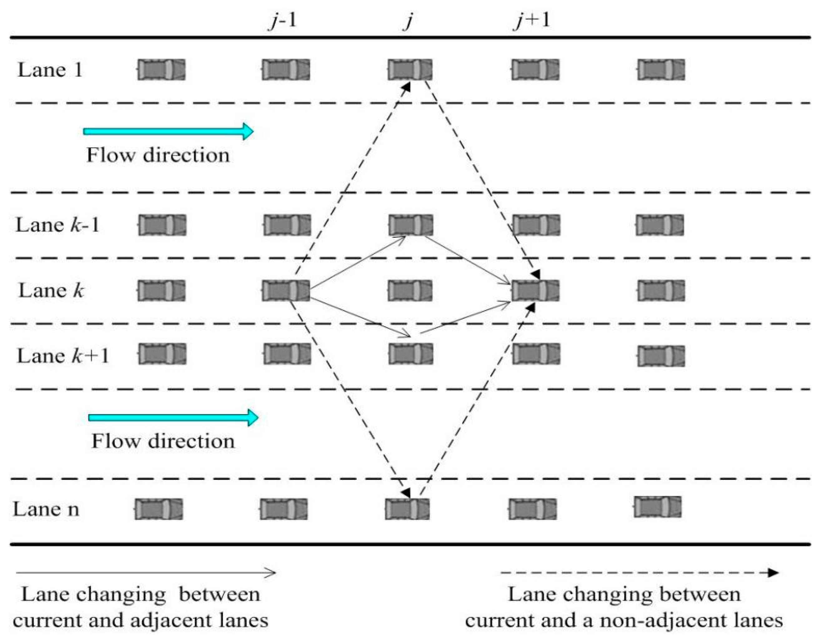
Figure 1. A schematic showing a multi-lane highway system where lane-switching actions are enabled by V2X technology [24]. In this new scenario, lane-switching actions are not limited to adjacent lanes, and cross-lane cooperative lane-changing maneuvers can also be performed.
Wevj 16 00457 g001
Figure 2. The schematic model of traffic flow on a two-lane highway [31].
Wevj 16 00457 g002
Figure 3. Phase diagram in the parameter space ( ρ , a ) under different values of k, with γ = 0.05 , n = 3.
Wevj 16 00457 g003
Figure 4. The phase diagram illustrates the variation relationship of the sensitivity coefficient with density ρ and the reaction coefficient k under the conditions of γ = 0.05 and n = 3.
Wevj 16 00457 g004
Figure 5. Phase diagram in the parameter space ( ρ , a ) under different values of n, with γ = 0.05 and k = 0.1.
Wevj 16 00457 g005
Figure 6. Schematic diagram of periodic boundary conditions.
Wevj 16 00457 g006
Figure 11. Plot of traffic density versus mean flux of traffic system for different values of k with a = 1.7 , γ = 0.05 , n = 3 . When k = 0 , the OEFDI information is not considered. As k > 0 , the OEFDI information is taken into account.
Wevj 16 00457 g011
Figure 12. Plot of traffic density versus mean flux of traffic system for different number of lanes n, with a = 2 , γ = 0.05 ,   k = 0.1 . For the purpose of comparison, the models proposed by Nagatani, Yang, and Peng are presented.
Wevj 16 00457 g012
Table 1. Critical sensitivity ac of our model and MS multi-lane lattice model for different n under γ = 0.05 .
n
1
2
3
4
Our modelac2.56202.30812.10001.9263
MS multi-lane lattice modelac32.72732.50002.3077
Table 2. A list of the key parameters in the new model.
NotationDefinitionUnit
NThe total number of road segments in the simulation system.-
jThe index of a roadway segment.-
aDriver’s sensitivity.s−1
tTime variable.s
τ Delay time in driver’s reaction, τ = 1 / a .s
ρ 0 The overall average density of the multi-lane system.veh/km
ρ c Critical density.veh/km
γ The lane-changing coefficient.-
n Number of lanes in multi-lane systems.-
kThe response coefficient associated with the OEFDI effect.s−1
VOptimized velocity function.km/h
v j ( t ) The average velocity at time t on the j -th segment in the multi-lane system.km/h
ρ j ( t ) The average density at time t on the j -th segment in the multi-lane system.veh/km
Disclaimer/Publisher’s Note: The statements, opinions and data contained in all publications are solely those of the individual author(s) and contributor(s) and not of MDPI and/or the editor(s). MDPI and/or the editor(s) disclaim responsibility for any injury to people or property resulting from any ideas, methods, instructions or products referred to in the content.