Abstract
To enhance the electromagnetic performance of flat-wire permanent magnet synchronous motors, three different groove structures were designed for the rotor, and a multi-objective optimization algorithm combining a genetic algorithm (GA) with the TOPSIS method was proposed. Firstly, an 8-pole 48-slot flat-wire motor model was established, and the cogging torque was analytically calculated to compare the motor’s performance under different groove schemes. Secondly, global multi-objective optimization of the rotor groove dimensions was performed using a combined simulation approach involving Maxwell, Workbench, and Optislang, and the optimal rotor groove size structure was selected using the TOPSIS method. Finally, a comparative analysis of the motor’s performance under both rated-load and no-load conditions was conducted for the pre- and post-optimization designs, followed by verification of the mechanical strength of the optimized rotor structure. The research results demonstrate that the combined optimization approach utilizing the genetic algorithm and the TOPSIS method significantly enhances the torque characteristics of the motor. The computational results indicate that the average torque is increased to 165.32 N·m, with the torque ripple reduced from 28.37% to 13.32% and the cogging torque decreased from 896.88 mN·m to 187.9 mN·m. Moreover, the total distortion rates of the air-gap magnetic flux density and the no-load back EMF are significantly suppressed, confirming the rationality of the proposed motor design.
1. Introduction
In recent years, as the energy crisis has deepened and the ecological environment has continued to deteriorate, energy conservation, efficiency improvements, and vibration and noise reduction have become research hotspots in the field of industrial motors [1,2,3]. Compared with other types of motors, PMSMs exhibit advantages such as a compact size, high efficiency, and a strong flux-weakening capability [4,5]. Among these, flat-wire PMSMs, featuring a unique long and flat rectangular winding structure, offer benefits including a high slot fill factor and a high power density, making them widely adopted in electric vehicles [6]. However, flat-wire PMSMs also suffer from drawbacks such as large torque ripple and electromagnetic vibrations, which can adversely affect the driving performance of electric vehicles. Consequently, enhancing the torque performance of flat-wire PMSMs has emerged as a significant research focus in recent years.
Reference [7] analyzes the AC loss characteristics of rectangular wire conductors under skin and proximity effects; compares the operational efficiency of rectangular-wire and round-wire motors under test conditions; and verifies the advantages of rectangular-wire motors in terms of their slot fill factor and efficiency range. However, this research neglected the end effects of the windings, resulting in discrepancies between the simulated and experimental calculations of the winding losses. Additionally, it did not comprehensively evaluate the motor’s electromagnetic performance, such as key indicators like average torque, torque ripple, and cogging torque. Reference [8] combines the advantages of rectangular wire windings and “V+1” type permanent magnets; optimizes the stator’s and the rotor’s structural parameters through a finite element analysis; and effectively reduces the torque ripple using a rotor auxiliary slot design. Nevertheless, this study does not explore the mechanical strength of rectangular wire windings at high speeds, the auxiliary slot design is not compared with other torque performance metrics, and the feasibility of multi-objective collaborative design optimization remains unexplored. Reference [9] addresses the issues of torque ripple and cogging torque in interior permanent magnet synchronous motors (IPMSMs) by implementing diverse rotor slotting designs. The optimal parameters are determined through parametric scanning and the NSGA-II multi-objective optimization algorithm. Reference [10] proposes an innovative rotor structure with trapezoidal slots. By employing an analytical approach, it derives a cogging torque calculation formula and elucidates the regulatory mechanism of the trapezoidal slot parameters on the pole arc coefficient and the air-gap magnetic field. Ultimately, it achieves a synergistic reduction in both the cogging torque and torque ripple. Reference [11] established a structural model of a flat-wire motor with hairpin windings and double-layer interior permanent magnets, utilizing the Taguchi optimization algorithm to determine the relationship between the dimensions of the double-layer permanent magnets and the output torque performance. The optimal dimensional combination for the double-layer permanent magnets was identified, ultimately achieving an increase in the motor’s average torque while simultaneously reducing torque ripple. Reference [12] enhances the torque characteristics of interior permanent magnet synchronous motors (IPMSMs) by optimizing the stator and rotor geometries. This study integrates Optimal Latin Hypercube Design (OLHD) and the Progressive Quadratic Response Surface Method (PQRSM) to construct the model, achieving a significant reduction in the torque ripple and cogging torque while maintaining the rated torque. The reliability of this model is validated through electromagnetic, demagnetization, and structural analyses. Reference [13] investigated the effect of rotor slotting on the torque performance by analyzing the impact of the slot position, with experimental validation confirming that this optimization method could effectively reduce torque ripple without affecting the other electromagnetic parameters. Reference [14] explored the segmentation of irregular slotting regions into smaller regular regions using calculus principles, establishing the relationship between the cogging torque and auxiliary slot parameters and verifying that stator tooth auxiliary slots could reduce the cogging torque. Reference [15] proposed a fast and accurate method for calculating the density of the radial electromagnetic force in surface-mounted permanent magnet synchronous motors (SPMSMs), focusing on the influence of different slot types (such as rectangular and arc-shaped slots near the stator teeth) and their quantities on the electromagnetic force and torque characteristics. However, after determining the rectangular slot shape, this study did not comprehensively consider the coupled effects of geometric parameters such as slot depth, slot width, and slot number on the multi-objective motor performance, neglecting potential complex interactions and multi-objective conflicts among these design variables. Furthermore, the key performance metric of the average torque was not included in the optimization objective system, resulting in limitations in the design dimensions. Reference [16] compared parallel tooth profiles with the traditional trapezoidal tooth profiles, proving that slot width and tooth shape could reduce the cogging torque in axial-flux permanent magnet motors. With ongoing research, references [17,18,19,20] have collectively demonstrated that the position, depth, and width of auxiliary slots significantly influence the reduction in cogging torque in motors.
In summary, improvements in motor torque performance primarily focus on stator–rotor slotting optimization and dimensional tuning of the permanent magnets, with most of these approaches employing analytical methods, finite element analyses, and Taguchi iterations to reduce the cogging torque and torque ripple [21]. However, the current research predominantly concentrates on round-wire winding motors, while optimization studies on the torque performance of hairpin-wound flat-wire motors remain relatively scarce. Therefore, this paper first analytically calculated the cogging torque in flat-wire motors to evaluate the torque performance of different groove designs. Secondly, a combined method incorporating a Genetic Optimization Algorithm + Sensitivity Analysis (Optislang) + TOPSIS + COWA was employed to optimize the dimensional structure of the combined rotor grooves. Finally, the electromagnetic characteristics before and after optimization were compared, and static simulations of the mechanical strength were performed to validate the rationality of the proposed design.
2. The Basic Structure of Flat-Wire Motors and the Rotor Groove Optimization Design
2.1. The Basic Structure of a Flat-Wire Motor
The flat-wire motor structure investigated in this study is illustrated in Figure 1a. The stator winding adopts a hairpin configuration which involves replacing the conventional round copper wire windings in the stator with long, flat rectangular windings that are inserted into the stator slots, as shown in Figure 1b. The rotor employs an interior-mounted “V+1” permanent magnet arrangement, with a pole–slot combination of 8 poles and 48 slots. The stator and rotor cores are made of DW310-35 silicon steel laminations, while the permanent magnets are grade N38UH sintered NdFeB. This motor structure features a simple design and reliable operation. Table 1 lists the main basic parameters of the motor.
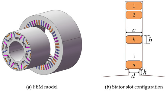
Figure 1.
Schematic of flat-wire motor structure.

Table 1.
Basic parameters of flat-wire motor.
2.2. Analysis of the Rotor Groove Design
This study takes the aforementioned flat-wire PMSM as the research subject, implementing slotting treatment on the rotor’s surface and analyzing the variations in the motor’s torque performance under different slot configurations. The slotting design on the rotor’s surface exclusively modifies the rotor’s magnetic reluctance without altering the size, position, or distribution of the permanent magnets. This implies that the rotor’s slotting design solely affects the cogging torque [22].
According to the energy method, cogging torque can be defined as the negative derivative of the magnetic field energy W with respect to the angular position α during no-load operation, expressed as
In the equation given, Tcog represents the cogging torque of the motor, W denotes the magnetic energy of the flat-wire PMSM under no-load conditions, and α is defined as the angular displacement between the center of the pole shoe and the corresponding stator tooth center.
The magnetic energy stored within the motor can be expressed as the air-gap magnetic energy, denoted as , as expressed by the following equation:
In the equation, Vq represents the volume between the stator slots and the rotor of the motor; B denotes the air-gap magnetic flux density of the stator teeth under no-load conditions; and µ0 is the permeability of the free space.
Under the assumption of a negligible drop in the magnetic voltage in ferromagnetic materials, the distribution of the air-gap magnetic flux density along the rotor’s surface exhibits a specific pattern characterized by
In the equation, Br(θ) represents the residual magnetic flux density function in the circumferential direction, h1(θ) denotes the magnetization thickness function along the circumference, and δg(θ,α) corresponds to the function of the air-gap length varying with the circumferential position.
Substituting Equation (3) into Equation (2) yields
After performing a Fourier transform on in the above equation and expanding the result, we obtain
In this equation, Tn represents the Fourier transform coefficient of the squared air-gap permeance; Z denotes the number of stator slots in the motor; and θ indicates the angular position relative to the pole shoe location, with θ = 0 defined as the center of the pole shoe.
After performing Fourier decomposition and transformation on , the expanded expression can be obtained:
In the equation given, αp represents the pole arc coefficient, Br denotes the remanent flux density of the permanent magnet, and n is a positive integer that ensures nZ/2p yields an integer value, where P is the number of pole pairs of the motor.
Based on the above analysis, the cogging torque of the flat-wire PMSM can be derived as follows:
In this equation, R1 represents the length of the outer diameter of the stator, and R2 denotes the length of the inner diameter of the rotor.
As derived from Equation (7), once the fundamental dimensions of the motor’s stator and rotor are determined, the cogging torque of the flat-wire motor is solely dependent on the parameter Bmz/2p. The rotor groove design significantly influences the magnetic flux density distribution, thereby altering the motor’s torque characteristics. Comparative analyses of the torque performance for different rotor groove design schemes are presented in Figure 2 and Figure 3.
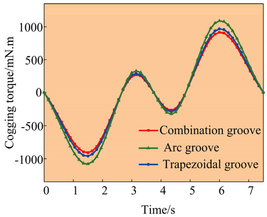
Figure 2.
Comparison of cogging torque under different slotting schemes.
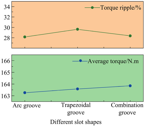
Figure 3.
Comparison of output torque performance under different slotting schemes.
As illustrated in Figure 2, both circular-arc groove and trapezoidal groove configurations of the motor rotor exhibit higher peak cogging torque values compared to those for the combined groove structure. Furthermore, as shown in Figure 3, the implementation of rotor grooving leads to a reduction in both the average torque and torque ripple under rated-load conditions. These findings demonstrate that different groove design schemes significantly influence the motor’s torque performance characteristics. Based on a comprehensive analysis of Figure 2 and Figure 3, the combined groove configuration featuring both circular-arc and trapezoidal grooves was selected as the optimal structural basis for subsequent multi-objective optimization.
3. Multi-Objective Optimization of the Rotor Combined Groove Structure in Flat-Wire PMSMs
3.1. The Rotor Combined Groove Structure in Flat-Wire Motors
To utilize the groove design on the rotor’s surface better to shift the phase of the cogging torque waveform, thereby reducing the peak cogging torque and the torque ripple in flat-wire motors, this work addresses the influence of combined rotor groove structures (including their position, depth, and width) on the motor’s torque output performance. As shown in Figure 4, the optimized configuration features alternating circular and trapezoidal grooves symmetrically distributed about the d-axis, with their center angles denoted as θ1 and θ2, respectively, their groove depths defined as h1 and h2, and the unified groove width represented by u. Specifically, the trapezoidal grooves are characterized further by their upper width (u1), middle width (u2), and lower width (u3) to precisely define their geometric features.
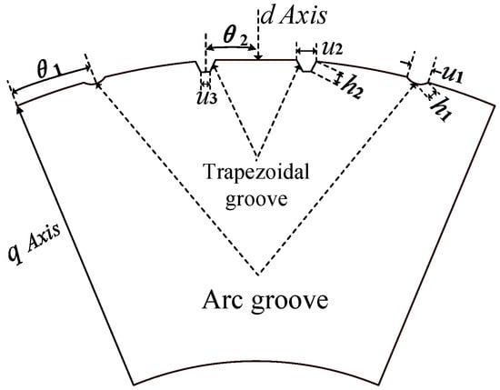
Figure 4.
A schematic diagram of the rotor auxiliary combination slot structure.
3.2. Optimization Variables and Sensitivity Analysis
The cogging torque and torque ripple of the motor can induce vibration and noise during operation and, in severe cases, may even degrade the operational stability of the motor while shortening its service life. The proposed optimization method aims to maximize the average torque output while simultaneously minimizing both the torque ripple and the peak values of the cogging torque. The initial parameter values and selected optimization ranges for the multi-objective optimization of the rotor’s combined grooves are presented in Table 2.
Table 2.
Value ranges and constraints of optimization variables.
To investigate the influence of individual dimensional variables in the rotor’s combined groove structure on the motor’s performance, a coupled finite element simulation was conducted using the sensitivity analysis (Optislong) module in ANSYS Workbench 2021 integrated with Maxwell 2023 software. The resulting sensitivity data, illustrating the impact of each dimensional parameter on the motor’s torque output performance, is presented in Figure 5.
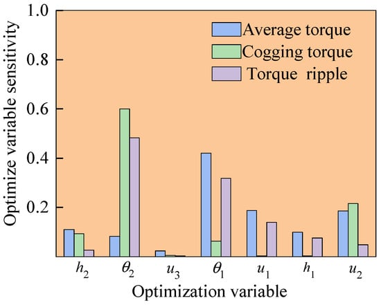
Figure 5.
Sensitivity analysis of optimization variables.
The magnitude of sensitivity indicates the degree of influence of each optimization variable on the torque performance optimization objectives [23]. As shown in Figure 5, the center position angle θ1 of the arc groove and the width u1 of the arc groove have the greatest impact on the motor’s average torque; the center position angle θ2 of the trapezoidal groove and the center position angle θ1 of the arc groove exhibit the most significant influence on the motor’s torque ripple; and the center position angle θ2 of the trapezoidal groove and the upper width u2 of the trapezoidal groove demonstrate the strongest effect on the motor’s cogging torque. Notably, the lower width u3 of the trapezoidal groove shows a minimal influence on all three performance metrics—average torque, torque ripple, and cogging torque. Consequently, it is necessary to perform multi-objective optimization on the remaining six variables: the center position angle θ1 of the arc groove, the center position angle θ2 of the trapezoidal groove, the width u1 of the arc groove, the depth h1 of the arc groove, the depth h2 of the trapezoidal groove, and the upper width u2 of the trapezoidal groove (excluding the less influential u3).
To investigate the patterns of influence of these six variables on the torque performance further, multivariate quadratic fitting was conducted based on response surface models of the three optimization objectives, focusing on the two most influential variables. A quadratic regression mathematical model was then established according to the finite element simulation results, as expressed in Equation (8).
In the equation, β0, βi, and βij represent the regression coefficients, where Xi and Xj denote the optimization variables, and α signifies the fitting error.
Therefore, the regression mathematical model of the average torque was established by fitting the circular arc groove center angle θ1 and the trapezoidal groove upper width u2 as the key parameters, while the torque ripple regression mathematical model was optimized using the circular arc groove center position angle θ1 and the trapezoidal groove center position angle θ2 as the design variables. The quadratic fitting mathematical model is expressed as Equation (9). Figure 6 and Figure 7, respectively, illustrate the surface response relationships between the motor’s average torque and torque ripple with respect to the design variables.
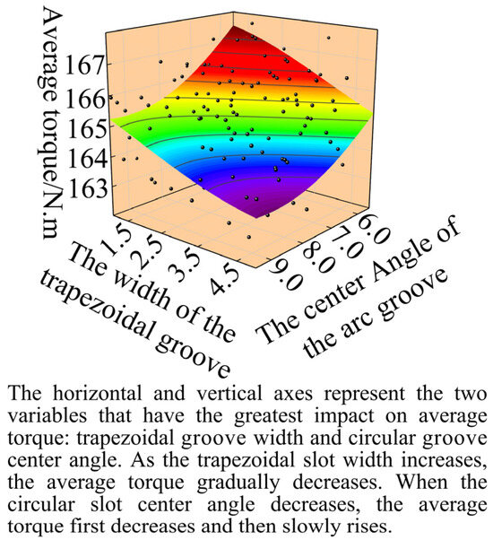
Figure 6.
Response surface fitting of average torque.
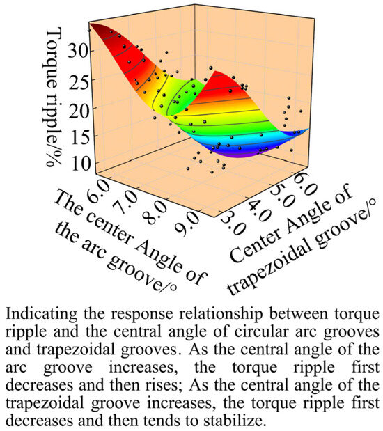
Figure 7.
Response surface fitting of torque ripple.
As illustrated in Figure 6, the average torque of the flat-wire permanent magnet synchronous motor exhibits significant variations with changes in the upper trapezoidal slot width (u2) and the central angle of the arc slot (θ1). Specifically, when the upper trapezoidal slot width (u2) increases, the average torque consistently decreases. Conversely, as the central angle of the arc slot (θ1) decreases, the average torque initially shows a gradual decline before experiencing a sharp increase. As shown in Figure 7, the torque ripple initially decreases and then increases sharply as the central angle of the arc groove (θ1) increases, which is particularly noticeable when the central angle of the trapezoidal groove (θ2) is small. As the central angle of the trapezoidal groove (θ2) continues to deviate, the torque ripple first decreases and then gradually stabilizes.
Furthermore, the cogging torque of the motor is most significantly influenced by the central position angle of the trapezoidal slot (θ2) and the upper trapezoidal slot width (u2). Taking u2 and u3 as the optimization variables for the mathematical model of cogging torque (as shown in Equation (10)), Figure 8 presents the surface response relationship between the motor’s cogging torque and the design variables, revealing their complex interaction effects on the torque performance.
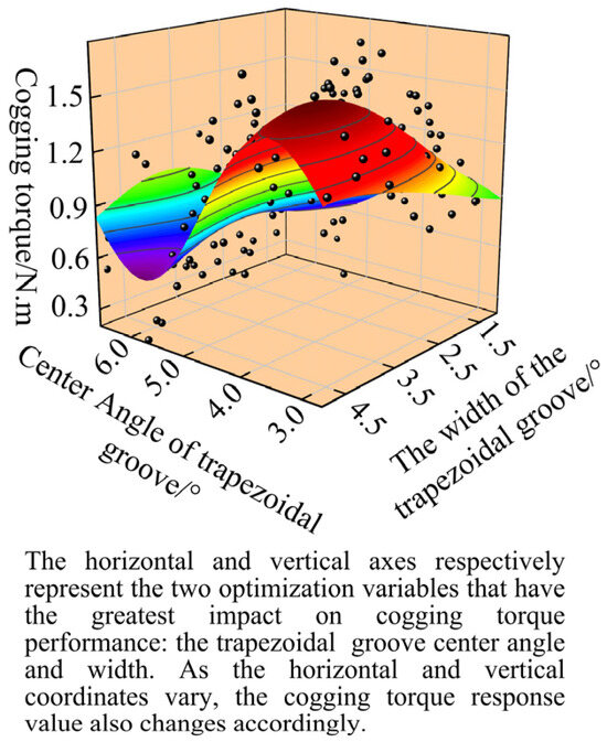
Figure 8.
Response surface fitting of cogging torque.
As illustrated in Figure 8, it can be observed that as the central angle θ2 of the trapezoidal groove progressively increases, the cogging torque initially rises and then experiences a sharp decline, followed by a gradual ascent—this trend becomes particularly pronounced when the upper slot width u2 of the trapezoidal groove is relatively large. When θ2 remains constant, the motor’s cogging torque Tcog exhibits an initial increase followed by a subsequent decrease as u2 decreases.
In summary, during the optimization of the combined groove parameters for the flat-wire motor rotor, the response surface formed by the optimization variables and the output values demonstrates highly complex characteristics, making it difficult to directly determine the optimal solution by examining individual variables. Therefore, a comprehensive evaluation of how each structural parameter for the rotor grooves influences the motor’s torque performance is essential. Ultimately, the dimensions of the optimal rotor groove structure should be selected based on this holistic analysis to achieve the best possible motor performance.
3.3. A Global Multi-Objective Joint Optimization Method Based on the GA and TOPSIS
The joint simulation optimization of the combined groove structure scheme for flat-wire motor rotors involves six optimization variables and three response parameters. The study begins by importing the 2D finite element model of the flat-wire motor from Maxwell into ANSYS Workbench to conduct a sensitivity analysis. The population size is set to 150 with a maximum iteration count of 100. The algorithm employs multi-point crossover and adaptive mutation, where the crossover probability and the mutation probability are configured as 0.7 and 0.12, respectively. Subsequently, a GA is employed to perform global multi-objective optimization of the motor’s torque performance, generating a globally optimal 3D Pareto solution set that establishes the relationship between the optimization variables and multiple performance objectives. Figure 9 presents a flowchart of the GA optimization process.
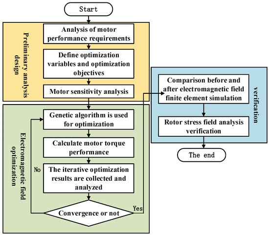
Figure 9.
Genetic algorithm (GA) optimization flowchart.
The optimization objectives were set to maximize the average torque while minimizing both the torque ripple and cogging torque, with specific target constraints applied as formulated in Equation (11).
In the equation, Tavg0, Tcog0, and Tripple0 represent the constraint threshold values for the motor’s average torque, cogging torque, and torque ripple, respectively.
The global multi-objective optimization results for the rotor’s combined groove structure are typically presented in the form of a Pareto front response surface, as illustrated in Figure 10. The distribution of the data points reflects the varying values of different optimization variables: light gray particles denote infeasible solutions that violate the predefined constraints, and dark gray particles represent feasible solutions within the constraint boundaries, while black particles indicate optimal solutions located on the Pareto frontier. The Pareto-optimal solutions are identified along this frontier, with the complete set of optimal solution data presented in Table 3.
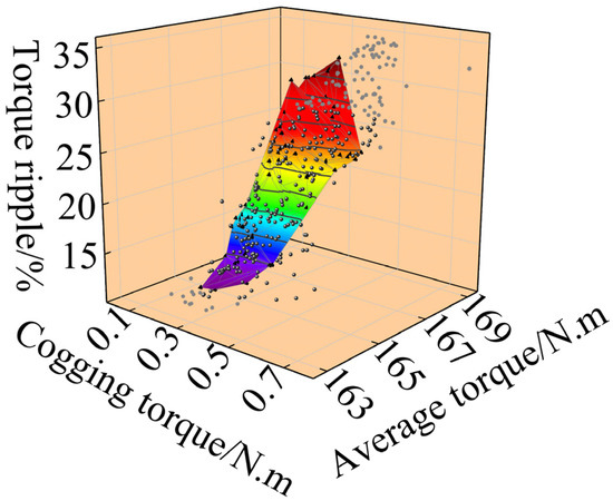
Figure 10.
Three-dimensional Pareto-optimal solution set.
Table 3.
Pareto-optimal solution set.
This study employs three optimization objectives as the evaluation metrics to assess the torque performance of flat-wire PMSMs. For the 3D Pareto-optimal solution set obtained using the GA, the interval combination number ordered weighted averaging (COWA) operator [24,25] is introduced. The objective weights for the three performance indicators—average torque, torque ripple, and cogging torque—are calculated, and the optimal solution set is weighted accordingly [26,27]. By computing the proximity index for each point in the optimal solution set to the optimal level, the solutions are ranked. The flowchart is shown in Figure 11. The specific evaluation process is as follows:
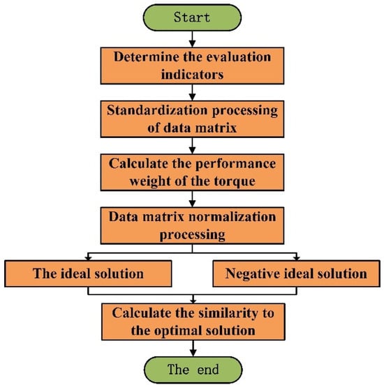
Figure 11.
Flowchart of TOPSIS method.
(1) The optimal solution set contains solutions. For the three performance indicators, a performance matrix A with t rows and three columns is constructed, which is then normalized:
Here, amn represents the Pareto-optimal value of each performance metric in the t-th row and the third column, where amax denotes the maximum Pareto value for each column of performance metrics.
(2) The weights δn of the three optimization objectives are calculated using the COWA operator:
In the equation, represents the combination number of selecting m − 1 elements from t − 1 elements.
(3) Based on the weight coefficients, the normalized performance matrix is assigned corresponding weights, where the weighted matrix K is constructed as follows:
(4) The maximum and minimum values of each column in the weighting matrix are identified. For the optimization objectives of the cogging torque and torque ripple, smaller values are always preferred, so the minimum value is defined as the positive ideal solution, while the maximum value serves as the negative ideal solution. Conversely, for the average torque optimization objective, larger values are more desirable, meaning its evaluation criteria are opposite to those for the other two objectives. Taking the cogging torque and torque ripple as examples, the following equation defines the positive and negative ideal solutions for these performance indices.
(5) Calculate the distances Zm+ and Zm− between each element in the weighted decision matrix and the positive ideal solution (PIS), as well as the negative ideal solution (NIS):
(6) The proximity index (Rm) was calculated to evaluate the closeness of each solution in the Pareto-optimal set to the ideal optimal level (a higher Rm value indicates a solution closer to the best achievable optimization result):
The average torque, torque ripple, and cogging torque were evaluated using Equation (14), with their respective weighting coefficients determined as 0.42999, 0.30654, and 0.26347 based on the multi-objective optimization criteria.
Based on the above process, the positive and negative ideal solutions under different evaluation indicators can be obtained, respectively, as shown in Table 4.
Table 4.
Positive and negative ideal solutions.
Based on the calculated positive and negative ideal solutions for different evaluation metrics, the distances from each alternative to these ideal solutions and their corresponding closeness coefficients were further determined, as presented in Table 5.
Table 5.
TOPSIS evaluation results.
According to Table 5, the solution with serial number 78 is the optimal result after this algorithm optimization, thereby determining the best structural parameters for the rotor grooves: the center angle of the arc groove θ1, the width of the arc groove u1, the depth of the arc groove h1, the trapezoidal groove’s center angle θ2, the trapezoidal groove’s top width u2, and the trapezoidal groove’s depth h2. The parameter values and optimization objectives before and after optimization using the genetic algorithm and Technique for Order Preference by Similarity to Ideal Solution (TOPSIS) are shown in Table 6.
Table 6.
Performance comparison before and after algorithm optimization.
As evidenced by Table 6, the optimization yields significant improvements in the motor’s torque performance, with the peak cogging torque reduced to 187.9 mN·m, the average torque under rated-load conditions increased to 165.32 N·m, and the torque ripple decreased to 13.32%.
4. Performance Verification and Analysis of the Optimized Motor
4.1. No-Load Performance Analysis
After performing global multi-objective optimization on the rotor groove dimensions using a combined GA and TOPSIS approach to selecting the optimal combined groove position and size configuration for the rotor, a finite element analysis (FEA) of the flat-wire motor under no-load conditions was conducted to verify the motor’s design rationality. The rationality of the mesh partitioning and boundary conditions directly determines the accuracy and reliability of the computational results. In this study, a refined mesh with a 0.1 mm element size was applied to the band domain, while master/slave boundary conditions were implemented on periodic symmetry planes. Figure 12 presents a comparative analysis of the cogging torque before and after motor optimization.
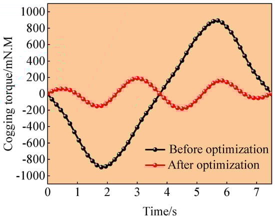
Figure 12.
Cogging torque comparison of flat-wire motors.
As illustrated in Figure 12, the joint simulation optimization using Maxwell, Workbench, and Optislang resulted in a significant reduction in the cogging torque in the flat-wire PMSM. The peak cogging torque decreased markedly from 896.88 mN·m before optimization to 187.9 mN·m after optimization. This substantial improvement effectively mitigates motor vibration and noise, thereby ensuring a smoother operational performance.
The air-gap magnetic flux density (MGFBD) significantly influences key performance metrics of the motor including its torque ripple, vibration noise, and service life. Figure 13 and Figure 14 present comparative visualizations of the air-gap magnetic flux density waveforms before and after optimization, along with their corresponding harmonic distribution spectra obtained through a Fourier analysis.
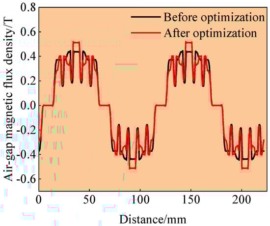
Figure 13.
Air-gap flux density waveform comparison of flat-wire motors.
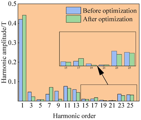
Figure 14.
Harmonic spectrum of air-gap flux density: baseline vs. optimized design.
As illustrated in the preceding figure, optimization led to an improvement in the fundamental amplitude of the MGFBD for the flat-wire PMSM, increasing from 0.42 T before optimization to 0.44 T after optimization. Furthermore, with the exception of the seventh harmonic component, all other harmonic amplitudes exhibit reductions compared to the pre-optimization state. The quantitative analysis demonstrates that the total harmonic distortion (THD) of the MGFBD decreases from 9.27% to 7.79% following optimization, achieving a 1.48% reduction in the distortion level. The distortion rate calculation follows the formulation presented in Equation (18).
where THD represents the total harmonic distortion rate, U1rms denotes the root mean square (RMS) value of the fundamental component obtained through a Fourier transform, and Unrms represents the RMS value of each harmonic component.
To validate the electromagnetic performance of the optimized flat-wire motor design further, the simulation results for the three-phase back EMF under no-load conditions and the harmonic distribution spectrum after Fourier decomposition are shown in Figure 15 and Figure 16, respectively.
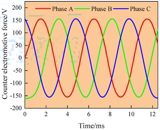
Figure 15.
The three-phase back EMF waveform of the motor.
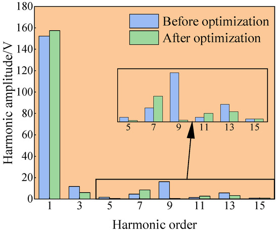
Figure 16.
Harmonic spectrum of back EMF: baseline vs. optimized design.
As illustrated in the preceding figure, the three-phase back EMF exhibit a periodic distribution with a consistent 120° phase difference between each phase, and their waveforms maintain an approximately sinusoidal distribution. The EMF waveforms meet the expected design requirements. Notably, while the content of the seventh harmonic shows a slight increase compared to the pre-optimization state, all of the other harmonic amplitudes demonstrate a significant improvement, with no evident waveform distortion observed and minimal high-order harmonic content. The quantitative analysis reveals that the no-load back EMF distortion rate was reduced from 5.368% before optimization to 2.741% after optimization, achieving a remarkable 2.627% reduction in the total harmonic distortion.
4.2. A Load Performance Analysis
Dimensional optimization of the rotor’s groove design not only modifies the motor’s cogging torque but also achieves a reduction in the torque ripple. Figure 17 compares the output torque performance under rated-load conditions before and after the optimization, demonstrating significant improvements in the torque characteristics.
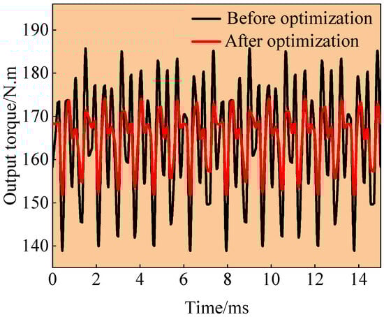
Figure 17.
Output torque performance comparison of flat-wire motors.
As illustrated in Figure 17, the torque ripple of the optimized flat-wire motor is significantly reduced by 15.05%, dropping from 28.37% to 13.32%, while the average output torque remains stable at approximately 165.32 N·m, meeting the expected design requirements.
Diagrams of the magnetic flux density contour and the magnetic field vector for the optimized flat-wire motor are presented in Figure 18 and Figure 19, respectively. These data analyses reveal that magnetic saturation primarily occurs in the rotor’s magnetic bridge isolation region, with no significant magnetic leakage detected. The magnetic flux density distribution demonstrates favorable characteristics, confirming that the motor’s structural design meets all of the specified requirements.
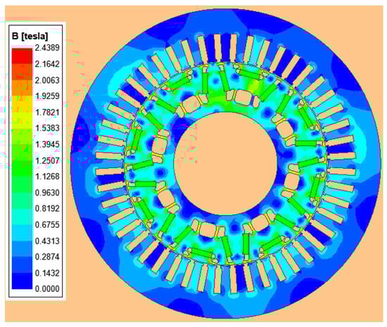
Figure 18.
The flux density contour of the optimized flat-wire motor under a load.
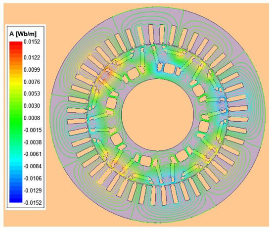
Figure 19.
A magnetic flux line vector plot for the optimized flat-wire motor under a load.
4.3. Verification of the Mechanical Strength of the Rotor
For flat-wire PMSMs operating at high speeds, the rotor stress increases proportionally with the rotational velocity. The designed rotor grooves exacerbate the stress concentration further, compromising the structural robustness of the rotor. Consequently, mechanical strength verification becomes essential to ensure the rotor’s integrity under high-speed conditions. To guarantee operational safety, the validation test was conducted at 1.2 times the motor’s peak rated speed, corresponding to 20,400 rpm. Figure 20 and Figure 21 present the von Mises stress distribution contour and the strain distribution map, respectively, of the optimized rotor under these elevated speed conditions.
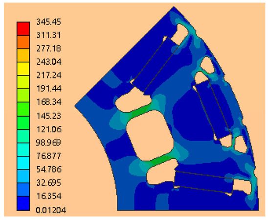
Figure 20.
Equivalent stress distribution contour of flat-wire motor rotor.
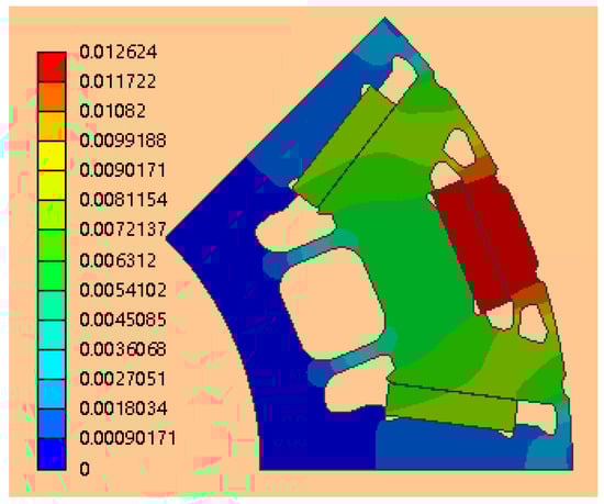
Figure 21.
Strain field plot of flat-wire motor rotor.
As evidenced by the preceding figures, during high-speed operation of the flat-wire motor, stress concentration primarily occurs in the magnetic bridge isolation region. The maximum equivalent stress reaches 345.45 MPa, which is significantly lower than the ultimate tensile strength of the rotor material (500 MPa). Furthermore, the maximum strain experienced by the rotor is approximately 0.012, well within the elastic deformation limit. Consequently, the optimized groove design of the rotor ensures reliable operation at peak rotational speeds.
5. Conclusions, Limitations, and Future Extensions
5.1. Conclusions
This paper presented the design of a hairpin-wound permanent magnet synchronous flat-wire motor for electric vehicle applications, where a two-dimensional finite element model of the motor was established. Analytical calculations were performed to evaluate the cogging torque of the flat-wire motor model, and three different rotor groove structures were designed. A multi-objective optimization algorithm combining a GA with the TOPSIS method was proposed. The main conclusions are as follows:
- (1)
- Three distinct rotor groove structures were developed for the flat-wire motor, and their torque performance was compared under various operating conditions. The data analysis shows that while the arc-shaped groove configuration exhibited a torque ripple of 28.16% under rated-load conditions—comparable to the combined groove design and superior to the trapezoidal groove’s 29.63%—the combined groove structure demonstrated significantly better average torque output and cogging torque characteristics. Based on a comprehensive evaluation across different operating conditions, the combined groove configuration was selected as the optimal rotor structure for subsequent multi-objective optimization.
- (2)
- To determine the optimal structural parameters for the rotor’s combined slots, global multi-objective optimization of the size structure of the rotor’s combined grooves was conducted using the combined method of a genetic algorithm + Optislang + TOPSIS + COWA, with the average torque, torque ripple, and cogging torque as the optimization objectives. The optimized results show remarkable improvements: the peak cogging torque was reduced from 896.88 mN·m to 187.9 mN·m; the torque ripple decreased from 28.37% to 13.32% (a 15.05% reduction); and the average torque increased steadily from 163.85 N·m to 165.32 N·m. Furthermore, the enhancement in the motor’s torque performance is accompanied by significant improvements in both the air-gap magnetic flux density characteristics and the back EMF distortion rate under no-load conditions. Prior to optimization, the fundamental amplitude of the air-gap magnetic flux density was measured at 0.42 T, which increased to 0.44 T after optimization, while its distortion rate was reduced from 9.27% to 7.79%. Simultaneously, the total harmonic distortion (THD) of the motor’s back electromotive force (EMF) was reduced from 5.368% before optimization to 2.741% after optimization, achieving a significant reduction of 2.627 percentage points.
5.2. Limitations and Future Extensions
Although this study provides valuable insights into the torque performance of hairpin motors under no-load and load conditions, its conclusions are entirely based on electromagnetic finite element simulation analyses and structural mechanics simulations, without experimental validation. While simulation methods can offer valuable theoretical guidance, the lack of experimental data still introduces certain limitations, as elaborated below:
Firstly, the demagnetization characteristics of permanent magnets are simplified in the simulation. In actual operation, high temperatures and local demagnetization may affect the magnetic field distribution after slotting. Moreover, in this study, the weighting factors for the improved cogging torque, average torque, and torque ripple performance were set as 0.4, 0.3, and 0.3, respectively. Alterations to these weighting factors will directly impact the motor’s operational performance. If the cogging torque weight is increased, it may optimize the low-speed smoothness, but the high-speed efficiency or noise could deteriorate. If the average torque weight is enhanced, this will improve the acceleration performance and load capacity but may sacrifice torque stability, leading to increased vibration. Meanwhile, emphasizing torque ripple reduction can lower the noise and vibration (NVH), improving ride comfort, but may compromise the power output efficiency. In practical applications, trade-offs between objectives are necessary. Urban commuter vehicles may prioritize torque ripple suppression to enhance comfort, while performance-oriented models may tend to favor the average torque to strengthen the power delivery. Fundamentally, weight adjustment represents a multi-objective (game) among efficiency, dynamic performance, and comfort, requiring balanced allocation based on the specific operational demands.
Secondly, the machining accuracy of rotor edge slots influences the consistency of the slot dimensions, which may lead to variations in the air-gap magnetic flux density distribution and consequently affect the electromagnetic performance. Additionally, slotting reduces the overall stiffness of the rotor structure. While simulations can calculate static stress, the fatigue characteristics under long-term high-speed operation cannot be accurately predicted through simulations alone.
In summary, incorporating a thermal field analysis and performing multiphysics coupling calculations using Maxwell + Fluent + Static Structural would enable a more comprehensive evaluation of the motor’s electromagnetic, mechanical, and thermal performance. Furthermore, if conditions permit, manufacturing a prototype and conducting experimental tests could effectively address the limitations of a simulation analysis. In constructing an electromagnetic performance test bench, high-precision torque sensors and encoders could be used to synchronously acquire dynamic torque signals, while a dynamometer could be employed to simulate actual operating conditions. The validation metrics include the torque ripple, average torque (the arithmetic mean under steady-state conditions), and cogging torque (measured through the no-load back-driving method). Additionally, the design optimization effect is quantified through a comparative analysis between finite element simulation and experimental data. This would provide critical data for calibrating the multiphysics model.
Author Contributions
Conceptualization: X.B. and H.Y.; methodology: X.B., Y.C. and W.H.; formal analysis: X.B., X.W. and M.L.; data curation: X.B.; writing—original draft preparation: X.B. and. Y.C.; writing—review and editing: X.B. and X.W.; visualization: M.L. and W.H.; supervision: H.Y. All authors have read and agreed to the published version of the manuscript.
Funding
This research was funded by National Natural Science Foundation of China (52305267); Natural Science Foundation of Shandong Province (ZR2022QE116); Key Laboratory of Precision Manufacturing and Special Processing in Shandong Province (90015322019).
Data Availability Statement
The original contributions presented in this study are included in the article; further inquiries can be directed to the corresponding author.
Conflicts of Interest
The author Hongbin Yin is an associate professor at Shandong University of Technology, and also a postdoctoral fellow jointly trained by Shandong University of Technology and China National Heavy Duty Truck Group Co., Ltd. The remaining authors declare that the research was conducted in the absence of any commercial or financial relationships that could be construed as a potential conflict of interest.
Abbreviations
The following abbreviations are used in this manuscript:
| GA | Genetic Algorithm |
| COWA | Comprehensive Objective Weighting Approach |
| THD | Total Harmonic Distortion |
| EMF | Electromotive Force |
References
- Aoyama, M.; Deng, J. Visualization and quantitative evaluation of eddy current loss in barwound type permanent magnet synchronous motor for mild hybrid vehicles. CES Trans. Electr. Mach. Syst. 2019, 3, 269–278. [Google Scholar] [CrossRef]
- Cai, W.; Wu, X.; Zhou, M.; Liang, Y.; Wang, Y. Review and development of electric motor systems and electric powertrains for new energy vehicles. Automot. Innov. 2021, 4, 3–22. [Google Scholar] [CrossRef]
- Adnane, M.; Nguyen, C.T.P.; Khoumsi, A.; Trovão, J.P.F. Real-time torque-distribution for dual-motor off-road vehicle using machine learning approach. IEEE Trans. Veh. Technol. 2024, 73, 4567–4577. [Google Scholar] [CrossRef]
- Ye, W.; Liu, Y.; Wu, G.; Wu, Q.; Chen, Z.; Chen, Z.; Li, Z.; Cao, Z. Design optimization and manufacture of permanent magnet synchronous motor for new energy vehicle. Energy Rep. 2022, 8, 631–641. [Google Scholar] [CrossRef]
- Muhammad, N.; Khan, F.; Ullah, B.; Alghamdi, B. Performance analysis and design optimization of asymmetric interior permanent magnet synchronous machine for electric vehicles applications. IET Electr. Power Appl. 2024, 18, 425–435. [Google Scholar] [CrossRef]
- Cakal, G.; Keysan, O. Axial flux generator with novel flat wire for direct-drive wind turbines. IET Renew. Power Gener. 2021, 15, 139–152. [Google Scholar] [CrossRef]
- Fang, H.; Chen, Q.; Wan, X.; Li, A. Design and Optimization of High Efficiency Flat wire Motor for Electric Vehicle. In Proceedings of the 2023 China Automation Congress (CAC), Chongqing, China, 17–19 November 2023; IEEE: New York, NY, USA, 2023; pp. 4102–4107. [Google Scholar]
- Lv, J.; Feng, H.; Zhang, H.; Xu, X.; Hua, W. Optimization and Characterisation of Flat-wire Permanent Magnet Motors for Electric Vehicles. In Proceedings of the 2024 IEEE Transportation Electrification Conference and Expo, Asia-Pacific (ITEC Asia-Pacific), Xi’an, China, 10–13 October 2024; IEEE: New York, NY, USA, 2024; pp. 411–416. [Google Scholar]
- Wu, S.; Tong, Y.; Tong, W. Research on Cogging Torque Suppression of Interior Tangential Permanent Magnet Synchronous Motor Based on Rotor Trapezoidal Slot Opening [J/OL]. Trans. China Electrotech. Soc. 2025; finalization. [Google Scholar] [CrossRef]
- Yang, Q.; Zhang, W.; Zhao, C. Research on Torque Performance of Marine Hybrid Excitation Synchronous Motors Based on PSO Optimization of Magnetic Permeability Structure. J. Mar. Sci. Eng. 2024, 12, 1064. [Google Scholar] [CrossRef]
- Xie, X.; Li, H.; Cai, W.; He, Z. Design and Research of a Double-layer Interior Permanent Magnet Synchronous Motor with Hairpin Winding. Electr. Mach. Control 2022, 26, 47–56. [Google Scholar] [CrossRef]
- Kim, H.J.; Baek, S.W. Optimal shape design to improve torque characteristics of interior permanent magnet synchronous motor for small electric vehicles. Microsyst. Technol. 2024, 31, 1203–1217. [Google Scholar] [CrossRef]
- Wang, L.; Wang, X. Torque Ripple Analysis and Reduction of Interior Permanent Magnet Synchronous Motors. IEEE Trans. Appl. Supercond. 2024, 34, 5206705. [Google Scholar] [CrossRef]
- Ni, Y.Y.; Cui, Z.S.; Wang, Q.J. Analytical modeling and optimization of a surface-mounted permanent magnet machine with auxiliary slots in rotor. Electr. Mach. Control 2021, 25, 65–71. [Google Scholar]
- Xing, Z.Z.; Wang, X.H.; Zhao, W.L. Research on weakening measure of radial electromagnetic force waves in permanent magnet synchronous motors by inserting auxiliary slots. Inst. Eng. Technol. Electr. Power Appl. 2020, 14, 1381–1395. [Google Scholar] [CrossRef]
- Wanjiku, J.; Khan, M.A.; Barendse, P.S.; Pillay, P. Influence of slot openings and tooth profile on cogging torque in axial-flux PM machines. IEEE Trans. Ind. Electron. 2015, 62, 7578–7589. [Google Scholar] [CrossRef]
- Gu, H.J.; Huang, W.M.; Wang, C.; Gao, J.W. Influence of stator teeth notching on cogging torque of interior permanent magnet motor. Electr. Mach. Control Appl. 2016, 43, 40–45. [Google Scholar]
- Zhang, Y.J.; Ye, Q.J.; Zhao, X.C.; Jiang, Z.; Zhu, J.A. Cogging torque reduction method of permanent magnet motor based on optimization of stator structure. Micromotors 2024, 57, 6–9+17. [Google Scholar]
- Yan, H.L.; Wu, Y.B.; Yang, Z.X.; Wang, Z.T. Effect of double slotting of the stator and rotor on the tooth torque of permanent magnet synchronous motors. Modul. Mach. Tool Autom. Manuf. Tech. 2023, 7, 166–170. [Google Scholar]
- Liang, J.W.; Liu, H.; Liu, X.P.; Wang, X.H.; Shen, L.H. Effect of stator tooth slotting on cogging torque of six-phase motor. Mach. Tool Hydraul. 2023, 51, 169–173. [Google Scholar]
- Perin, D.; Karaoglan, A.D.; Yilmaz, K. Rotor design optimization of a 4000 rpm permanent magnet synchronous generator using moth flame optimization algorithm. Int. J. Optim. Control Theor. Appl. (IJOCTA) 2024, 14, 123–133. [Google Scholar] [CrossRef]
- Xu, S.; Zhang, X.; Wang, P.; Wang, C.; Li, X. A method for reducing cogging torque in interior permanent magnet synchronous motors of electric vehicles. China Sci. 2020, 15, 942–947. [Google Scholar]
- Zhu, X.; Fan, D.; Mo, L.; Chen, Y.; Quan, L. Multi objective optimization design of a double-rotor flux-switching permanent magnet machine considering multimode operation. IEEE Trans. Ind. Electron. 2019, 66, 641–653. [Google Scholar] [CrossRef]
- Tang, H.C.; Yang, S.T. Optimizing three-dimensional constrained ordered weighted averaging aggregation problem with bounded variables. Mathematics 2018, 6, 172. [Google Scholar] [CrossRef]
- Jin, F.; Ni, Z.; Chen, H.; Li, Y.; Zhou, L. Multiple attribute group decision making based on interval-valued hesitant fuzzy information measures. Comput. Ind. Eng. 2016, 101, 103–115. [Google Scholar] [CrossRef]
- Hu, Y.; Wu, L.; Shi, C.; Wang, Y.; Zhu, F. Research on optimal decision-making of cloud manufacturing service provider based on grey correlation analysis and TOPSIS. Int. J. Prod. Res. 2020, 58, 748–757. [Google Scholar] [CrossRef]
- Kannan, V.S.; Lenin, K.; Navneethakrishnan, P. Machining parameters optimization in laser beam machining for micro elliptical profiles using TOPSIS method. Mater. Today Proc. 2020, 21 Pt 1, 727–730. [Google Scholar] [CrossRef]
Disclaimer/Publisher’s Note: The statements, opinions and data contained in all publications are solely those of the individual author(s) and contributor(s) and not of MDPI and/or the editor(s). MDPI and/or the editor(s) disclaim responsibility for any injury to people or property resulting from any ideas, methods, instructions or products referred to in the content. |
© 2025 by the authors. Published by MDPI on behalf of the World Electric Vehicle Association. Licensee MDPI, Basel, Switzerland. This article is an open access article distributed under the terms and conditions of the Creative Commons Attribution (CC BY) license (https://creativecommons.org/licenses/by/4.0/).