An Enhanced ABS Braking Control System with Autonomous Vehicle Stopping

Abstract

This study explores the design and implementation of a control system integrating the anti-lock braking system (ABS) with frequency-modulated continuous wave (FMCW) radar technology to enhance safety and performance in autonomous vehicles. The proposed system employs a hybrid fuzzy logic controller (FLC) and proportional-integral-derivative (PID) controller to improve braking efficiency and vehicle stability under diverse driving conditions. Simulation results showed significant enhancements in stopping performance across various road conditions. The integrated system exhibited a marked improvement in braking performance, achieving significantly shorter stopping distances across all evaluated surface conditions—including dry concrete, wet asphalt, snowy roads, and icy roads—compared with scenarios without ABS. These results highlight the system’s ability to dynamically adapt braking forces to different conditions, significantly improving safety and stability for autonomous vehicles. The limitations are acknowledged, and directions for real-world validation are outlined to ensure system robustness under diverse environmental conditions.

1. Introduction

Autonomous driving technology has emerged as a promising solution to enhance traffic efficiency, reduce accident rates, and alleviate congestion, particularly with the growing adoption of electric vehicles [1,2,3,4]. Autonomous vehicles (AVs) operate in complex and unpredictable traffic environments, necessitating reliable and robust control systems [1,5]. A critical aspect of these systems is their ability to perform accurate and safe stopping under various conditions, ensuring the safety of passengers and pedestrians alike. Traditional braking systems, such as anti-lock braking systems (ABSs), have significantly improved safety by preventing wheel lock-up during sudden braking and maintaining steering control. However, the increasing autonomy of vehicles demands advanced braking systems that can integrate seamlessly with sensors and control units for real-time decision-making. FMCW (frequency-modulated continuous wave) radar technology provides high-resolution data on distance and velocity, making it highly suitable for real-time obstacle detection and braking control. This integration can address the challenges of modern autonomous systems by enhancing responsiveness and safety across diverse driving scenarios. This research aims to develop an integrated control system that combines ABS with FMCW radar to improve stopping performance and safety in autonomous vehicles. The project focuses on designing innovative algorithms to reduce stopping distances, enhance braking precision, and adapt to diverse road and weather conditions. It also emphasizes improving emergency braking stability by synchronizing radar detection with ABS performance. Through simulation and system integration, the study seeks to contribute to the development of safer and more reliable autonomous vehicles. This research holds significant importance in advancing the safety and efficiency of self-driving vehicles by developing an integrated control system that combines FMCW radar technology with anti-lock braking systems (ABSs). The integration of these technologies provides a more reliable and precise mechanism for detecting obstacles and executing braking maneuvers, especially under challenging conditions such as adverse weather, high speeds, and heavy traffic. By enhancing stopping performance and ensuring greater responsiveness, this study supports the progression of autonomous vehicle technology, contributing to the development of safer, more efficient, and dependable transportation systems.

This research adopts a structured methodology to design, implement, and evaluate an integrated control system for autonomous vehicle stopping. It begins with a detailed literature review on FMCW radar, ABSs, and stopping systems, focusing on their integration and challenges. A comprehensive system architecture is developed, alongside control algorithms for obstacle detection, braking force optimization, and ABS activation. Performance evaluation is conducted through an experimental platform, utilizing simulations or a test vehicle under diverse conditions. Data analysis assesses system effectiveness, supported by simulations to validate performance before real-world testing. The findings highlight limitations, propose enhancements, and provide a foundation for future advancements in autonomous stopping systems.

Recent studies have focused their efforts on improving and developing anti-lock braking systems (ABSs), where these systems are integrated with various strategies aimed at enhancing overall driving safety and efficiency. Through these studies, innovative solutions are being explored that contribute to enhancing vehicle performance and improving the driving experience, which helps reduce potential risks and accidents. Moloto and Nyandoro reviewed wheel slip control strategies, employing optimal control and feedback linearization techniques, which significantly improved braking efficiency under diverse driving conditions [6]. Similarly, El-Bakkouri et al. developed a torque distribution algorithm for electric vehicles, balancing frictional and regenerative braking, resulting in substantial improvements in energy recovery and vehicle stability [7]. Furthermore, Perez et al. utilized spiking neural networks to create a real-time adaptive ABS, which enhanced dynamic control and minimized wheel lock-ups [8]. In another advancement, Chen et al. proposed a neural network-based ABS control system, maintaining optimal slip ratios and demonstrating superior performance in challenging driving environments [9]. Additionally, Al-Mola et al. combined active force control with a fuzzy-tuned PID system, improving braking response and vehicle stability in dynamic conditions [10]. Haris et al. further contributed by designing a self-tuning PID controller, which enhanced slip control precision and braking performance in real-time scenarios [11]. In the field of FMCW radar technologies, recent research has emphasized improving radar performance and accuracy in complex environments. Reitz and Künzle examined FMCW radar performance in dense environments, proposing strategies to mitigate interference and improve detection accuracy [12]. Similarly, Guo et al. developed an advanced CMOS-based radar processor, enhancing data processing speeds and energy efficiency, making it highly suitable for autonomous systems [13]. Wang et al. introduced a non-contact radar system for biometric monitoring, showcasing its potential in new applications with high precision [14]. Quan et al. integrated obstacle detection with a fuzzy logic controller to improve interaction with dynamic obstacles, enhancing autonomous braking systems’ performance [15]. Additionally, Sadeghi et al. demonstrated the potential of mm-FMCW radars in monitoring vital signs under complex conditions, highlighting their versatility in autonomous and health applications [16]. Moreover, other studies have focused on improving the synergy between radar technologies and control systems. Rao et al. applied deep learning techniques to mmWave radars, significantly enhancing localization accuracy for autonomous vehicles [17]. Gatti et al. developed a dual-mode radar for environmental monitoring, demonstrating its effectiveness in precise navigation and object detection [18]. Lastly, Reitz et al. emphasized the role of FMCW radars in improving system reliability in dense industrial and traffic scenarios [12]. Razavi et al. [19] highlighted the importance of considering the broader implications for urban planning, societal integration, and eco-friendly transportation in addition to the control system’s efficiency. This research situates technical braking methods within a broader interdisciplinary framework, recognizing that ensuring safe and dependable AV functioning is essential for sustainable transportation. Beyond technical aspects, human elements such as a driver’s readiness to take over and their trust in automated systems, alongside regulatory aspects like liability laws and remote operation guidelines, are crucial for successful implementation.

These studies demonstrate the potential of integrating ABS with various technologies to enhance the design of safer driving systems, especially under changing environmental conditions. This knowledge provides a strong foundation for developing the system proposed in this research.

2. Anti-Lock Braking System (ABS)

During hard braking, wheel lock-up reduces vehicle stability and increases risks to occupants [20]. The ABS prevents lock-up by adjusting wheel slip to maintain optimal friction, improving stability, reducing braking distance, and preserving steering control [21]. ABS modulates braking torque based on the wheel slip coefficient to maintain effective wheel–road friction. Wheel slip, the relative motion between the wheel and road surface, occurs when the wheel’s angular velocity deviates from its free-running speed [22].

2.1. Subsection

ABSs are typically modeled mathematically, and they include speed sensors, a control unit, and actuators. This model helps assess system performance under various conditions. Calibration using parameters such as braking pressure decrease, restoration rates, and threshold speed values enhances system performance [23]. Three main components make up vehicle modeling: vehicle dynamics, wheel dynamics, and system braking dynamics. Figure 1 shows the forces that a vehicle is subject to upon braking.

If the vehicle brakes in a uniform, rectilinear motion, the equilibrium equation may be expressed as follows:

F_i = F_f

(1)

where F_f is the friction force between wheel and the road surface and F_i is the moving inertia force of the vehicle. Total normal force may be stated as follows:

F_N = m_v × g

(2)

where m_v is the total mass of the vehicle and g is the gravitational acceleration. Substituting this into Coulomb’s friction law, the friction force becomes

F_f = µ(λ) × m_v × g

(3)

where μ(λ) is the road adhesion coefficient. The moving inertia force is the product of the mass of the car m_v [kg] and the acceleration of the car α_v:

$${\mathrm{F}}_{\mathrm{i}}={\mathrm{m}}_{\mathrm{v}} \times {\alpha }_{\mathrm{v}}={\mathrm{m}}_{\mathrm{v}} \times \dot{\mathrm{V}\mathrm{v}}$$

(4)

where $\dot{\mathrm{V}\mathrm{v}}$ is the linear speed of the vehicle. Thus, the vehicle acceleration during braking is

V_v = −µ(λ) × g

(5)

By integration of Equation (5), we obtain the vehicle speed.

2.1.1. Wheel Dynamics Model

Provided the wheel is stiff and the road surface reaction is passed via the hub, the driver generates torque in the opposite direction of the wheel radius by applying braking torque to the wheels [23]. Figure 1 shows the forces applied to a vehicle’s wheel when it is braking.

Consequently, we develop the subsequent equation for wheel dynamics. The equation of motion for the rotational DOF at wheel level, as per Newton’s second law, is given by

J_w × ω_ω = T_b − T_t

(6)

where T_t is the tire torque, which can be mathematically stated as follows:

$${\mathrm{T}}_{\mathrm{t}}={\mathrm{F}}_{\mathrm{f}} \times { \mathrm{R}}_{\mathrm{r}}=\mu \left(\lambda \right) \times {\mathrm{F}}_{\mathrm{N}} {\times \mathrm{R}}_{\mathrm{r}}$$

(7)

Then

$${\mathrm{T}}_{\mathrm{b}}-{\mathrm{F}}_{\mathrm{f}} \times { \mathrm{R}}_{\mathrm{r}} - {\mathrm{J}}_{\omega }\times {\displaystyle \frac{\mathrm{d}{\omega }_{\omega }}{\mathrm{dt}}}=0$$

(8)

where J_ω is wheel moment of inertia, ω_ω is wheel speed, R_r is wheel radius, T_b is braking torque, and F_f is road friction force.

Given Equation (10) we obtain the formula for wheel acceleration

$${\displaystyle \frac{\mathrm{d}{\omega }_{\omega }}{\mathrm{dt}}}={\displaystyle \frac{1}{{\mathrm{J}}_{\omega }}}({\mathrm{T}}_{\mathrm{b}} - {\mathrm{F}}_{\mathrm{f}} \times { \mathrm{R}}_{\mathrm{r}})$$

(9)

To find the equation of wheel speed, we integrate of the following Equation (9).

2.1.2. Relative Slip

The ABS must control relative slip around an optimal goal. The relative slip equation is written as

$$\delta =1 - \frac{{\omega }_{\omega }}{{\omega }_{\mathrm{v}}}$$

(10)

where ω_ω is the angular speed of the wheel and ω_v is the angular speed of the vehicle. The wheel angular speed is calculated

$${\omega }_{\omega }={\displaystyle \frac{{\mathrm{T}}_{\mathrm{t}} - {\mathrm{T}}_{\mathrm{b}}}{{\mathrm{J}}_{\omega }}}$$

(11)

and vehicle angular speed is calculated

$${\omega }_{\mathrm{v}}={\displaystyle \frac{{\mathrm{V}}_{\mathrm{v}}}{{\mathrm{R}}_{\mathrm{r}}}}$$

(12)

where T_t is tire torque, T_b is the braking torque, and J_ω is the wheel rotational inertia.

2.1.3. Slip Ratio

The slip ratio is the difference between the vehicle linear speed and the wheel angular speed, indicated by (λ). It is created as

$$\lambda ={\displaystyle \frac{{\mathrm{V}}_{\mathrm{v}} - {\mathrm{R}}_{\mathrm{r}} \times {\omega }_{\omega }}{{\mathrm{V}}_{\mathrm{v}}}}$$

(13)

2.1.4. Slip Rate

Differentiating the equation above with respect to time (t), we get

$$\dot{\lambda }={\displaystyle \frac{{\dot{\mathrm{V}}}_{\mathrm{v}}\left(1 - \lambda \right) - {\mathrm{R}}_{\mathrm{r}} \times \dot{{ \omega }_{\omega }}}{{\mathrm{V}}_{\mathrm{v}}}}$$

(14)

where V_v is the vehicle linear speed, R_r is the wheel radius, and ω_ω is the wheel angular speed.

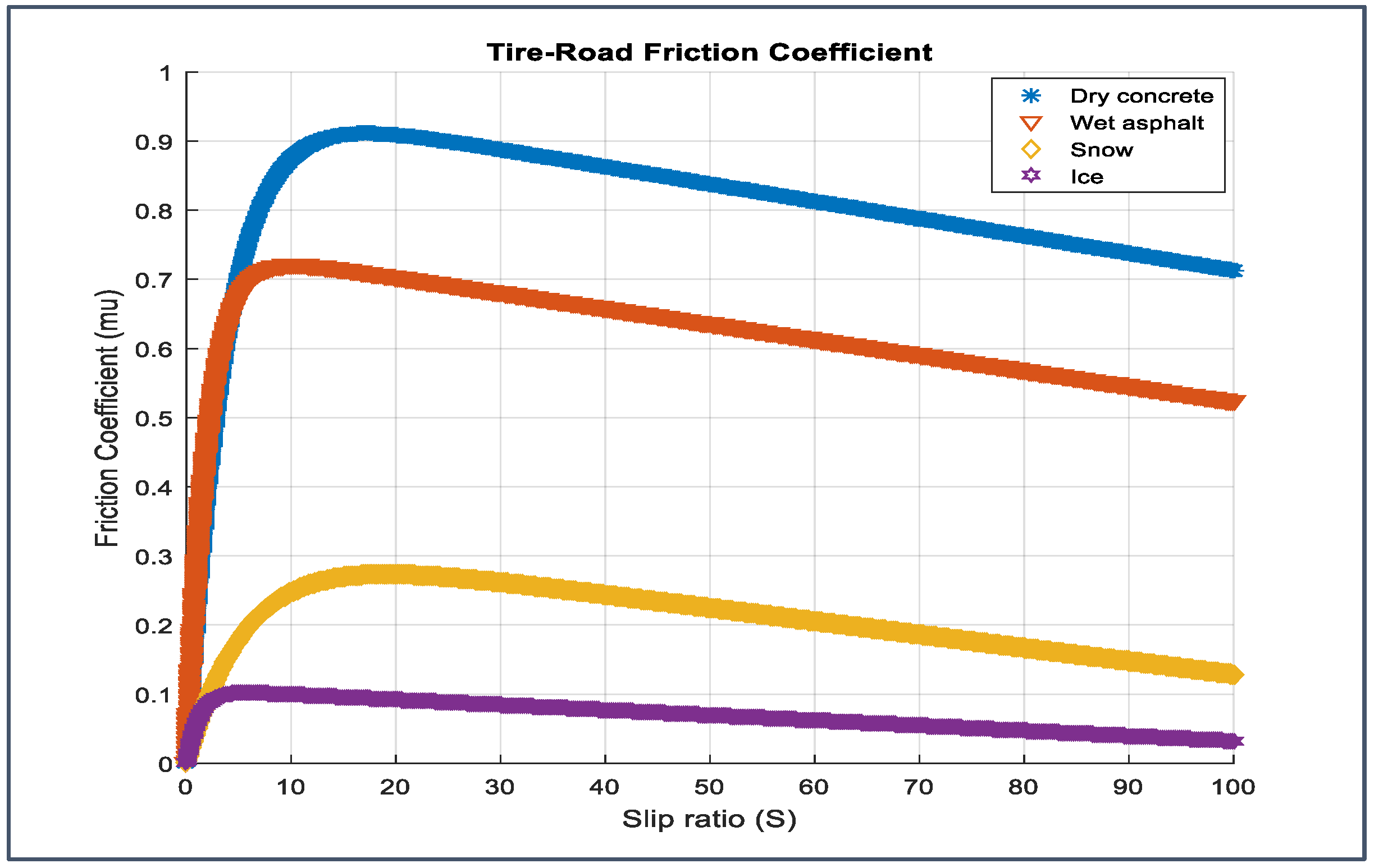
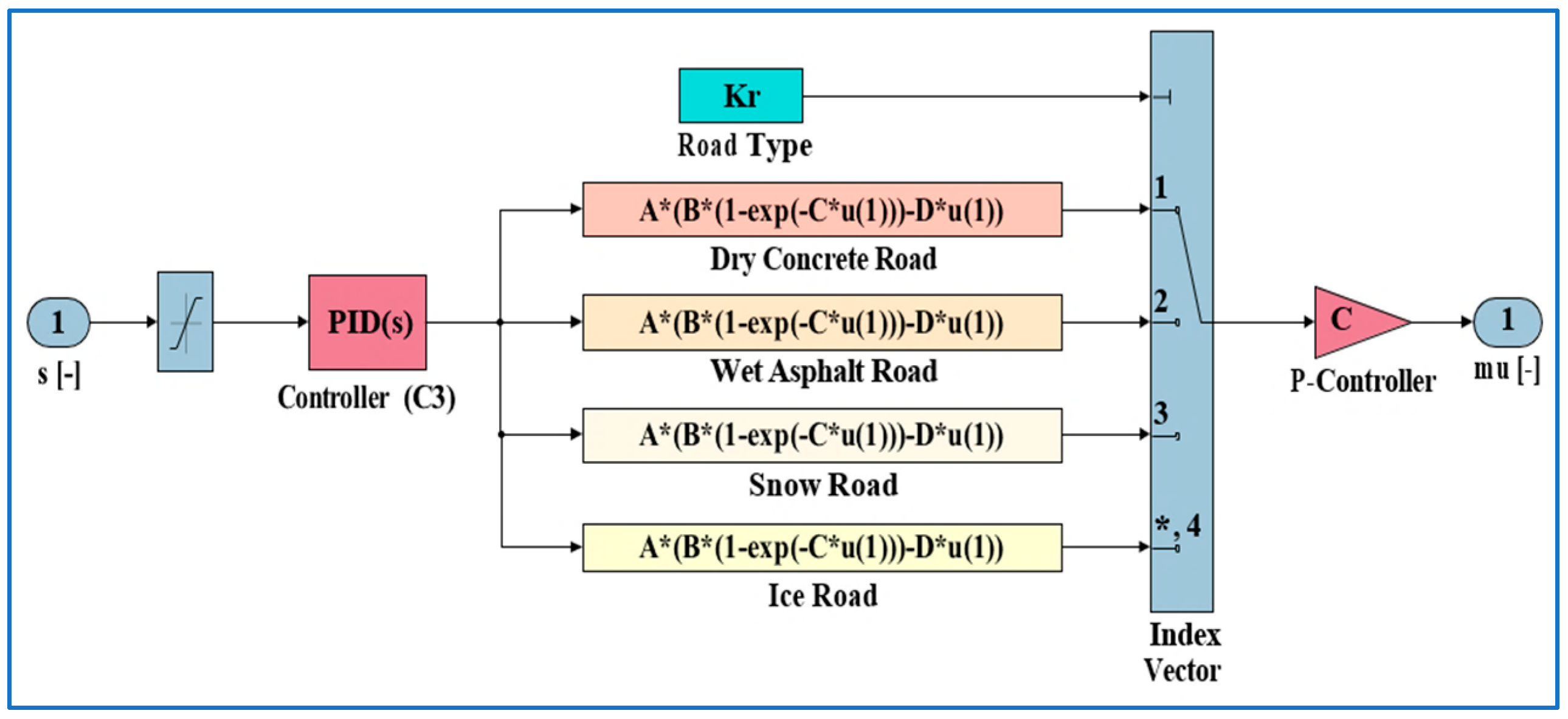
2.2. Model of Burckhardt

Burckhardt’s model is utilized to determine the tire-road friction coefficient, as expressed in the following equation

$$\mu \left(\lambda \right)=\mathrm{A}·(\mathrm{B}·\left(1-{\mathrm{e}}^{-\left(\mathrm{C}·\lambda \right)} - \mathrm{D} · \lambda \right))$$

(15)

where λ represents the wheel slip, and the coefficients A, B, C, and D define the friction levels based on road conditions.

Table 1. Coefficient for Burckhardt Model.

	Coefficients	A	B	C	D
Types of Roads
Dry concrete		0.9	1.07	0.2723	0.0026
Wet asphalt		0.7	1.07	0.5	0.003
Snow		0.3	1.07	0.1773	0.006
Ice		0.1	1.07	0.83	0.007

presents the corresponding values for different surface types, contributing to vehicle control simulations aimed at improving stability and safety.

Figure 2 displays simulation-generated curves based on Equation (15), illustrating the variation of friction with slip initially increasing, reaching a peak, and then declining. Each surface type has a unique friction curve, with dry surfaces offering the highest friction and icy surfaces the lowest, impacting vehicle stability.

2.3. Parameters Used in the ABS Model

Table 2. Parameters used in the ABS model.

Symbol	Value	Description
$m_v$	1200 [kg]	Total vehicle mass
$J_{\omega }$	5 [kg·m2]	Wheel inertia
$R_r$	0.36 [m]	Wheel radius
$v_0$	30 [m/s]	Initial vehicle speed
F	$m_v\times g$ [N]	Normal force (weight)
${\omega }_0$	$v_0/Rr$ [rad/s]	Wheel speed angular
g	9.81 [m/s2]	Gravitational acceleration
$K_f$	1 [-]	Force and Torque
${PB}_{max}$	2000 [N·m]	Maximum braking torque applied to the wheels
TB	0.01 [s]	Hydraulic Lag
${\lambda }_d$	0.2 [-]	Desired slip
Ctrl	1 or 0	With ABS $\to 1$ and Without ABS $\to 0$
K	1200	Proportional gain
A, B, C, and D	-	The constants which depend on road conditions
Road type	1, 2… N	Constant for road setting
e	2.2204 × 10−16	Division by zero protection constant

presents parameters for simulating the ABS model, including vehicle mass, wheel inertia, radius, speed, braking torque, slip ratio, and road/control constants, crucial for accurate ABS performance assessment.

2.4. Simulation of ABS Model

The simulation model integrates the ABS, control unit, and tire–road interaction to prevent wheel lock-up and enhance safety. Figure 3 visually depicts the interactions between these components, illustrating the data and control signal flow for an efficient and responsive braking system.

2.4.1. Simulation of Wheel Model

Figure 4 presents a basic wheel model, illustrating the relationships among components affecting wheel motion. It highlights the importance of understanding these interactions to improve braking systems, suspension design, and vehicle performance, contributing to safer, more efficient vehicles. The background colors indicate distinct functional components of the braking system model: blue represents input/output signal blocks, orange corresponds to dynamic system elements and actuators, and pink highlights torque-related processes or effects.

2.4.2. Simulation Model Friction

The simulation model includes a friction unit simulating four road types: dry concrete, wet asphalt, snow, and ice, with each having a specific friction coefficient. It uses a road coefficient parameter for realistic simulation and combines PID and P controllers to adjust brake force based on road conditions. Figure 5 demonstrates the model’s ability to predict frictional forces and adapt vehicle behavior, making it useful for vehicle control system simulations. The red block represents the dry concrete road model, the beige block corresponds to the wet asphalt road model, the light-yellow block indicates the snow road model, and the light green block denotes the ice road model. The cyan block labeled "Kr" represents the road type selector, while the pink block shows the PID controller. Light blue is used for signal processing and index vector elements.

3. ABS Controller

The proposed ABS controller integrates three key components to improve system performance: the PID unit for precise wheel speed control, the FLC unit to adapt to nonlinear conditions using fuzzy rules, and the saturation unit to maintain stability by limiting output values and preventing overshoot. This combination ensures efficient and safe ABS operation under varying driving conditions.

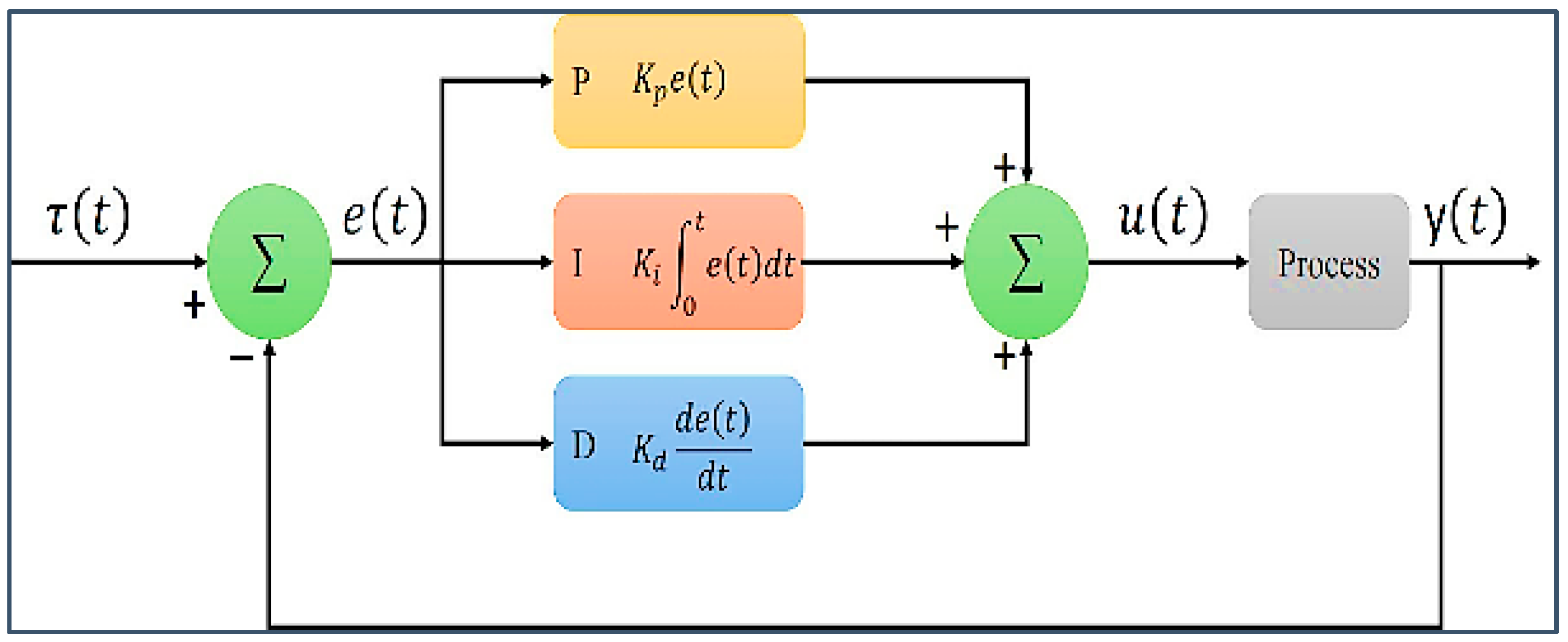
3.1. PID Controllers

PID controllers, a type of feedback control system, are widely used in motor control systems [24,25,26,27]. The system consists of three sub controllers: Proportional (P), Integral (I), and Derivative (D), which together form the PID control structure. Although PID is typically a continuous-time controller, it must be adapted for discrete-time operation in microcontroller systems. The system compares the target and actual values, calculates the error, and generates a control signal to correct it. Figure 6 illustrates the block diagram of the PID control system. In Figure 6 The error is calculated in the green summing block, representing the difference between the target and the actual output. This error is processed through three parallel paths: the yellow block is the Proportional controller which reacts to the current error, the orange block is the Integral controller which corrects for accumulated past errors, and the blue block is the Derivative controller which predicts future behavior by analyzing how the error is changing. These three signals are combined in another green summing block to produce the control signal. This signal is sent to the grey block, which represents the process being controlled, and the resulting output is continuously fed back into the loop to maintain stable and accurate system behavior.

The estimated control input for the system is shown in the following equation:

$$u\left(\mathrm{t}\right)={\mathrm{K}}_{\mathrm{p}}\mathrm{e}\left(\mathrm{t}\right)+{\mathrm{K}}_{\mathrm{i}}{\int }_0^{\mathrm{t}}\mathrm{e}\left(\mathrm{t}\right)\mathrm{dt}+{\mathrm{K}}_{\mathrm{d}}{\displaystyle \frac{\mathrm{de}\left(\mathrm{t}\right)}{\mathrm{dt}}}$$

(16)

where τ(t) is the control inputs, and K_p, K_i, and K_d are the coefficients of proportional, integral, and deviation terms, respectively.

Simulation of PID by MATLAB

In the MATLAB R2019a (v9.6) simulation of the PID controller, the Proportional component adjusts for current errors, the Integral component addresses long-term errors, and the Derivative component anticipates future errors to enhance stability and minimize overshoot. The simulation optimizes PID parameters for efficient brake control in the ABS model, as shown in Figure 7. The input passes first to the Proportional Controller shown in light blue, which multiplies the signal by a proportional gain to respond instantly to the input. Simultaneously, the signal enters the Integral Controller shown in light red, where it is scaled and then integrated by the Integrator in peach red, helping eliminate accumulated error over time. In the third path, the Derivative Controller shown in light pink calculates the rate of change of the input using the Derivative block in pale peach, predicting future trends. These three outputs are then summed together in the light blue vertical “Add” block to produce the final output signal.

3.2. Simulation of PID Controller by MATLAB

L.A. Zadeh introduced fuzzy theory in 1965, emphasizing simple control over precision. Fuzzy sets assign a degree of membership, unlike classical sets [28]. Fuzzy logic aids in power flow solutions by characterizing data in an arithmetic progression, optimizing congestion levels, and reducing design complexity [29,30]. It simplifies decision-making with predefined tolerance limits and minimizes computational efforts, optimizing power flow and electrical parameters in restructured power systems.

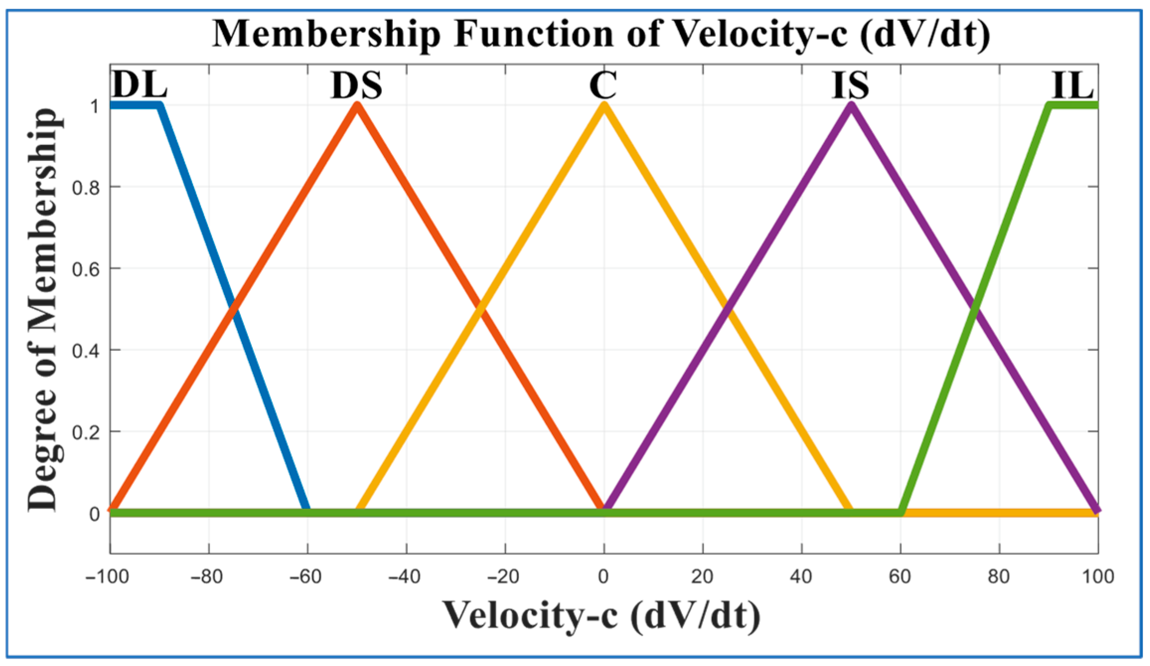
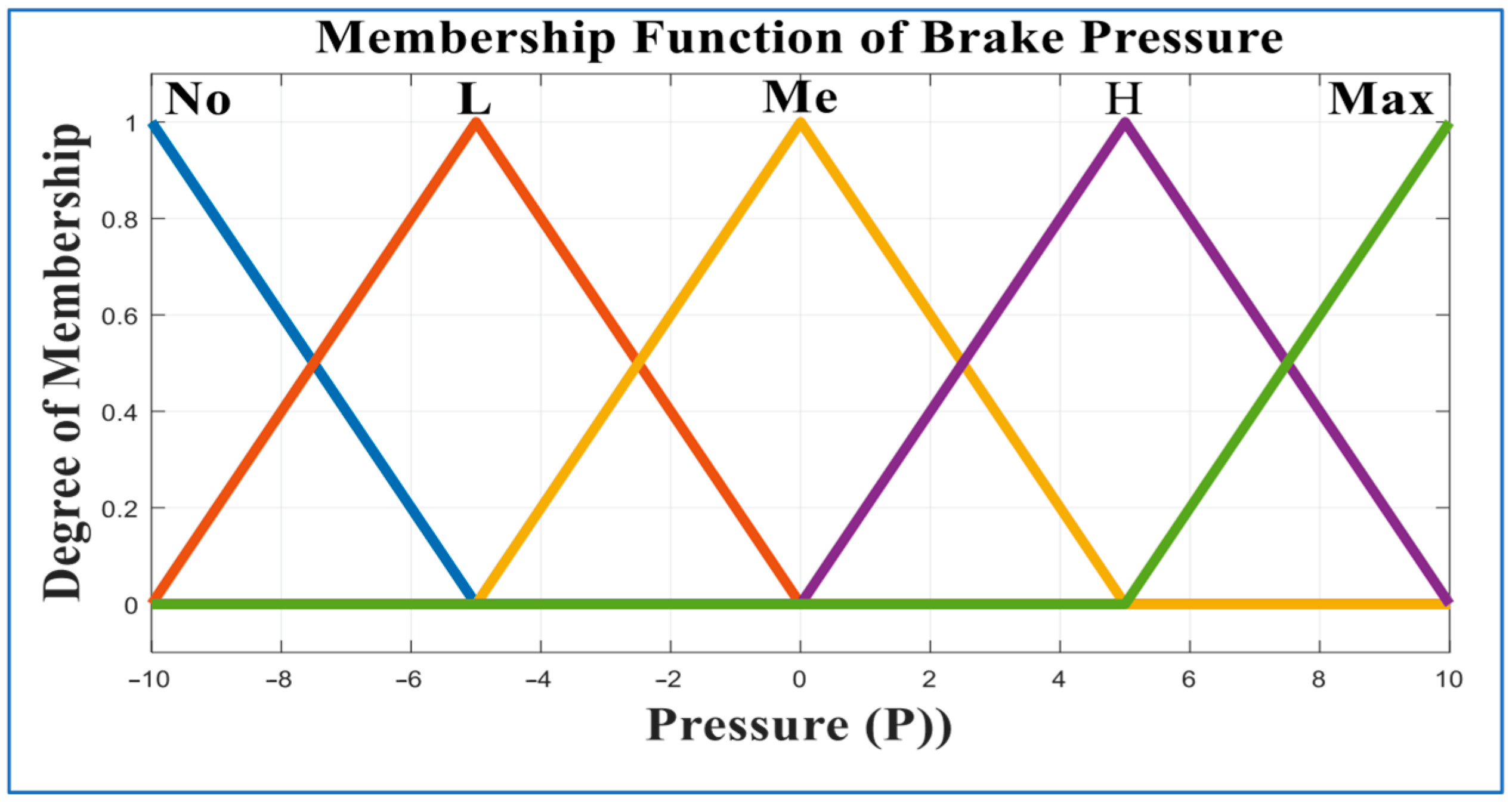
3.2.1. Simulation of FLC by MATLAB

The FLC is a viable method for increasing ABS performance due to its ability to manage complicated dynamics, uncertainties, and erroneous inputs. MATLAB, with its comprehensive computing and visualization capabilities, is a suitable environment for modeling FLC-based ABSs.

• Inputs and outputs: The inputs and outputs to the controller are as follows:
  • Input 1: The error of slip between actual slip and the reference slip (error).
  • Input 2: The error change ration (error-c).
  • Output: The braking pressure (pressure).
• Membership Functions: The number of membership functions (MFs) depends on the linguistic values used. In our case, for velocity (V), five categories are defined: Low (L), Medium (Me), High (H), Very High (VH), and Maximum (Max), as shown in Figure 8, Figure 9 and Figure 10. Each category describes the degree of participation for a given velocity. The velocity (V) membership function in a fuzzy logic system is shown in Figure 8.

Figure 9 shows acceleration as velocity changes over time, classified into five categories: decreasing low (DL), decreasing slow (DS), constant (C), increasing slow (IS), and increasing low (IL). The membership function helps fuzzy systems interpret velocity for decision-making.

Figure 10 shows the brake pressure membership function, using five categories to describe pressure levels: none (No), low (L), medium (Me), high (H), and maximum (Max). The membership degree indicates the extent to which a brake pressure value belongs to each category.

3.2.2. Rule Table

Table 3. Fuzzy inference mapping for 5 × 5 rules.

	Velocity-c	DL	DS	C	IS	IL
Velocity
L		No	No	No	No	L
Me		No	L	Me	Me	Me
H		Me	Me	H	Me	Me
VH		H	Max	Max	H	H
Max		Max	Max	Max	H	H

displays a 25-rule fuzzy table that employs two input variables, each of which has five membership sets. In fuzzy control applications, the 5 × 5 inference matrix makes accurate inferences and manages complicated system behaviors efficiently by determining output values depending on input circumstances.

The fuzzy logic rules in the ABS control system adjust brake pressure based on vehicle velocity and wheel speed differences, ensuring stability and preventing lock-up under varying road and driving conditions.

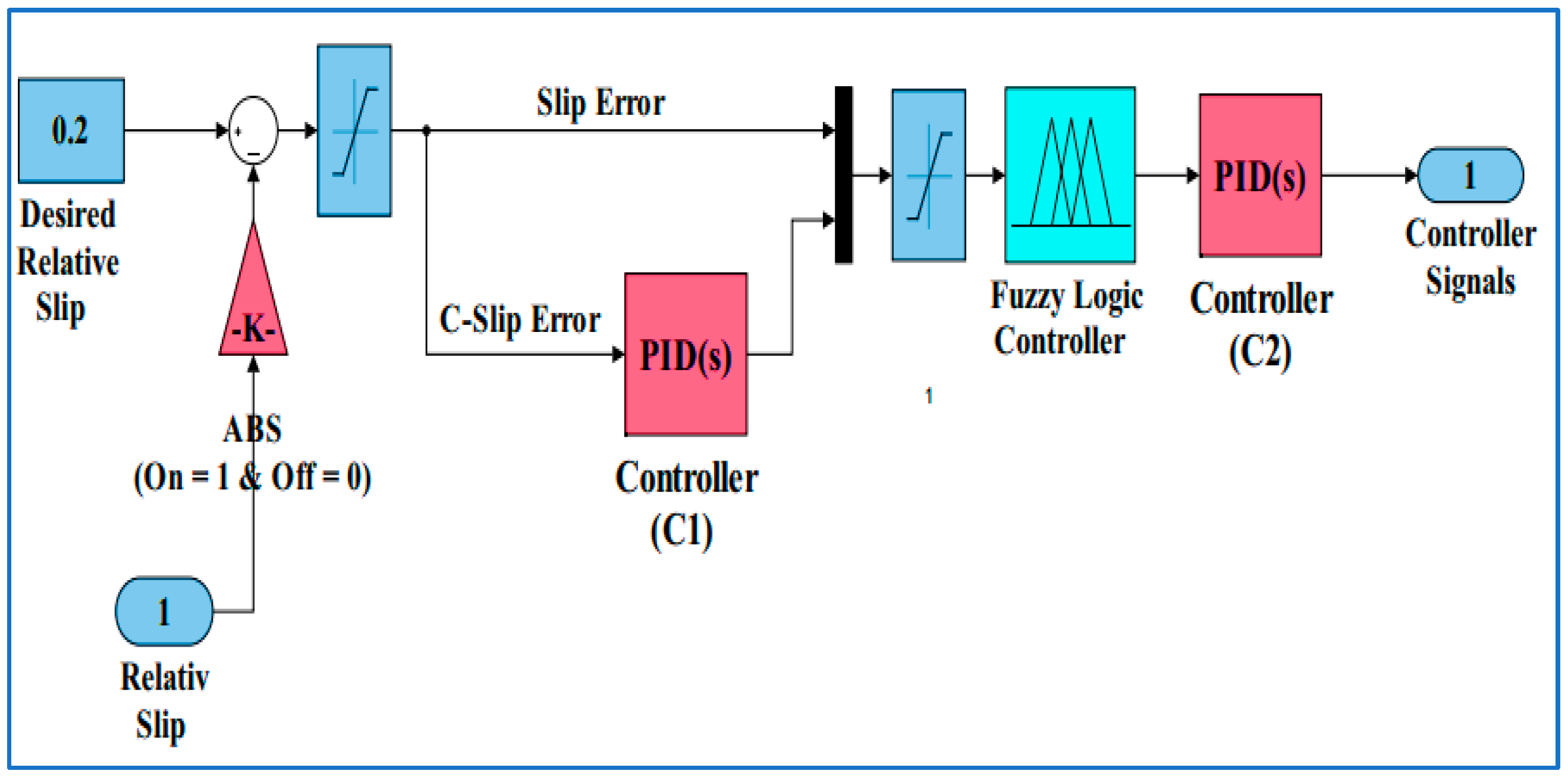
3.3. Simulation of ABS Controller

The ABS controller unit consists of a fuzzy logic module, two PID controllers, and a saturation coefficient. The fuzzy logic improves adaptability, the PID controllers ensure precise brake force control, and the saturation coefficient prevents excessive braking. This setup optimizes wheel slip ratios, enhancing vehicle safety. Figure 11 shows the ABS controller simulation. The background colors in the figure represent different categories of components within the ABS control system model. Blue indicates input/output signals, red denotes PID controllers, and cyan highlights the fuzzy logic controller.

4. Frequency Modulation Continuous Wave Radar (FMCW)

The FMCW Radar Measurement Principle, developed by Christian Hülsmeyer in 1904, is a technique used for detecting, locating, measuring speed, and characterizing objects through electromagnetic waves. Radar systems are categorized into pulsed and continuous wave (CW) types, with FMCW radars measuring both distance and speed by detecting frequency shifts. These radars, known for their ability to detect multiple targets simultaneously, are widely used in applications such as autonomous driving, radar altimeters, remote sensing, synthetic-aperture radar imaging, level gauging, air surveillance, and automotive navigation [31]. The technology used by automotive radar systems is known as frequency-modulated continuous wave (FMCW). Figure 12 shows a schematic that has been simplified.

FMCW Radar Standards cover frequency-modulated continuous wave radar. A radar uses a continuous carrier modulated by a periodic function, such as a sinusoid or sawtooth wave, to provide range data. Figure 13 shows the FMCW idea. Transmitters send linear frequency-modulated signals. The objects will reflect the signals, which will be detected by the receiver. The frequency offset between the receiving signal (Rx Sig.) and the transmitting signal (Tx Sig.) indicates the distance and speed of the objects [32].

The symbols are as follows: T is the chirp’s modulation period, B is the bandwidth for frequency sweeps, f₀ is the transmitted signal’s central frequency, f_v is the shift in doppler frequency, f_r is a shift in range frequency, f_bu = f_r − f_v is the ascending ramp’s beat frequency, f_bd = f_r + f_v is the beat frequency for the down ramp. The values of f_bu and f_bd are computed using a sampled down-converted receive signal. The object’s range and velocity may then be determined using the equations below.

$$\mathrm{R}=\left({\displaystyle \frac{\mathrm{c} ·\mathrm{T}}{4 ·\mathrm{B}}}\right)\left({\displaystyle \frac{{\mathrm{f}}_{\mathrm{bu}}+{\mathrm{f}}_{\mathrm{bd}}}{2}}\right)$$

(17)

$$\mathrm{v}=\left({\displaystyle \frac{\mathrm{c} }{2 · {\mathrm{f}}_0}}\right)\left({\displaystyle \frac{{\mathrm{f}}_{\mathrm{bu}}-{\mathrm{f}}_{\mathrm{bd}}}{2}}\right)$$

(18)

where R is range of the object, v is relative velocity of the object, and c is a velocity of the light.

Automotive radar sensors play a crucial role in advanced driver assistance systems (ADAS) and modern autonomous vehicles due to their low-cost hardware, ability to operate effectively in adverse weather conditions, and resilience in poor visibility. Most practical automotive radar systems utilize frequency-modulated continuous wave (FMCW) signals in the millimeter-wave band, enabling cost-effective, high-resolution sensing required for complex autonomous driving functions such as automatic emergency braking, blind-spot detection, and adaptive cruise control. However, the widespread deployment of radars operating within the 76–81 GHz frequency band, particularly in dense traffic environments, has raised significant concerns about mutual interference between radar systems [33]. FMCW radars are frequently used in industrial applications, especially for short-range measurements, because to their low cost, simplicity of use, and accurate range and velocity readings. They have various applications in vehicle accident prevention systems. Their ability to detect range and velocity even in unfavorable weather conditions makes them an attractive topic in autonomous vehicle research [34,35].

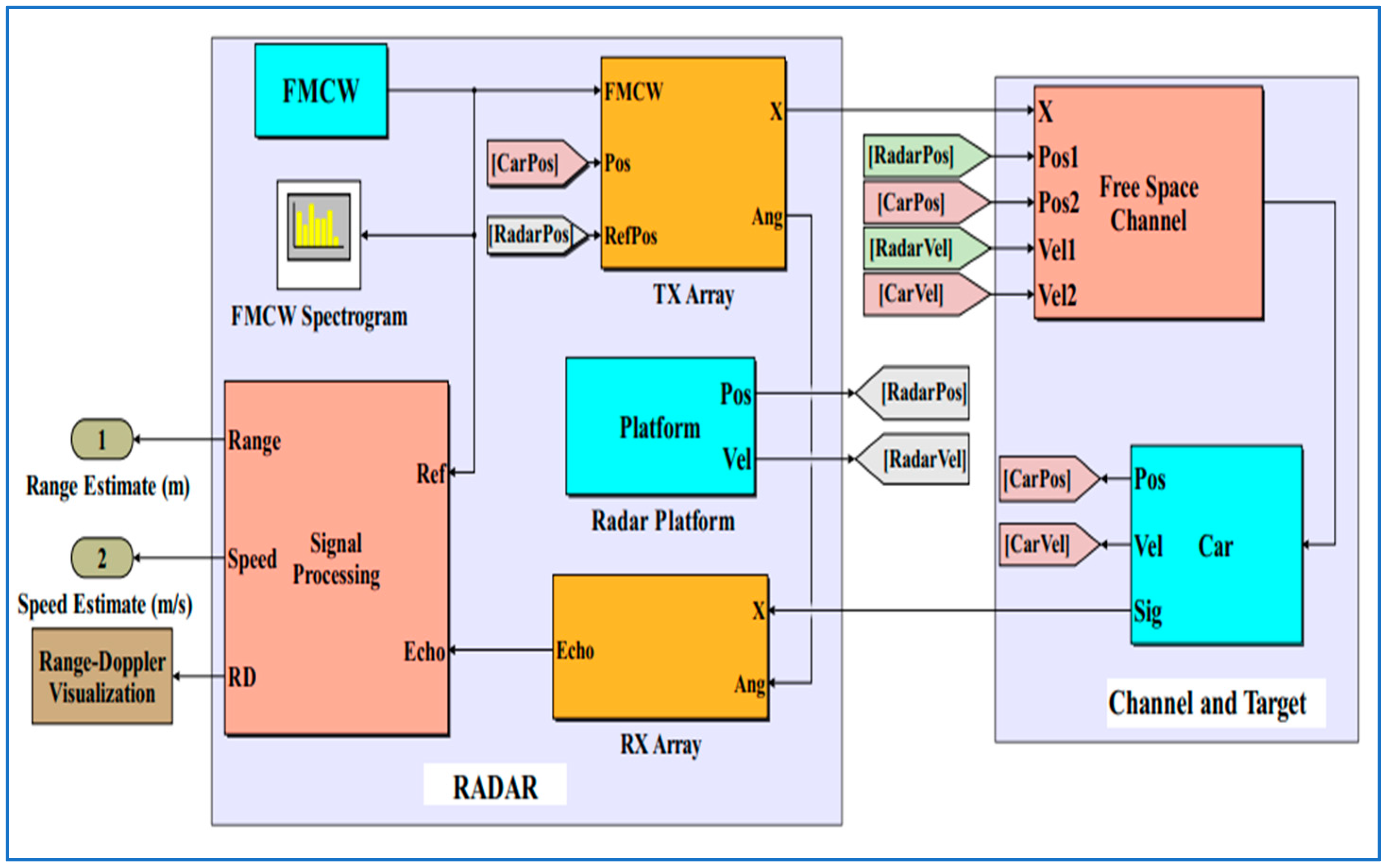
4.1. FMCW Radar Model

The FMCW radar model is a sophisticated radar system that uses frequency modulation to precisely determine the distance and speed of objects, making it essential for environmental sensing and detection. Our implementation leverages radar-based state estimation to detect relative velocity and distance, essential for precise braking control.

Recent studies have advanced FMCW radar’s capabilities through improved signal processing pipelines and dual-domain filtering techniques [36]. We integrated similar signal conditioning strategies to reduce interference and improve object detection. Sensor fusion mechanisms also benefit from work on multi-target detection under complex traffic conditions [36], which were considered in refining our fusion algorithm.

4.1.1. Simulation of Radar

The radar system simulation in Figure 14 shows its main components: a signal generator, an antenna for signal transmission and reception, and a processing unit for analyzing reflected signals. The radar detects multiple objects, estimates their distance, and calculates their relative speed. This data is essential for the autonomous braking system to adjust braking force accurately and in a timely manner, enhancing vehicle safety and functionality. Light blue represents control or platform modules such as the FMCW block, Radar Platform, and Car. Orange indicates array components involved in signal transmission and reception, including the TX and RX Arrays. Pink is used for dynamic processing blocks like Signal Processing and the Free Space Channel. Light brown highlights user interface elements, such as the Range-Doppler Visualization. Light purple is used to group major subsystems, including the RADAR and Channel and Target sections.

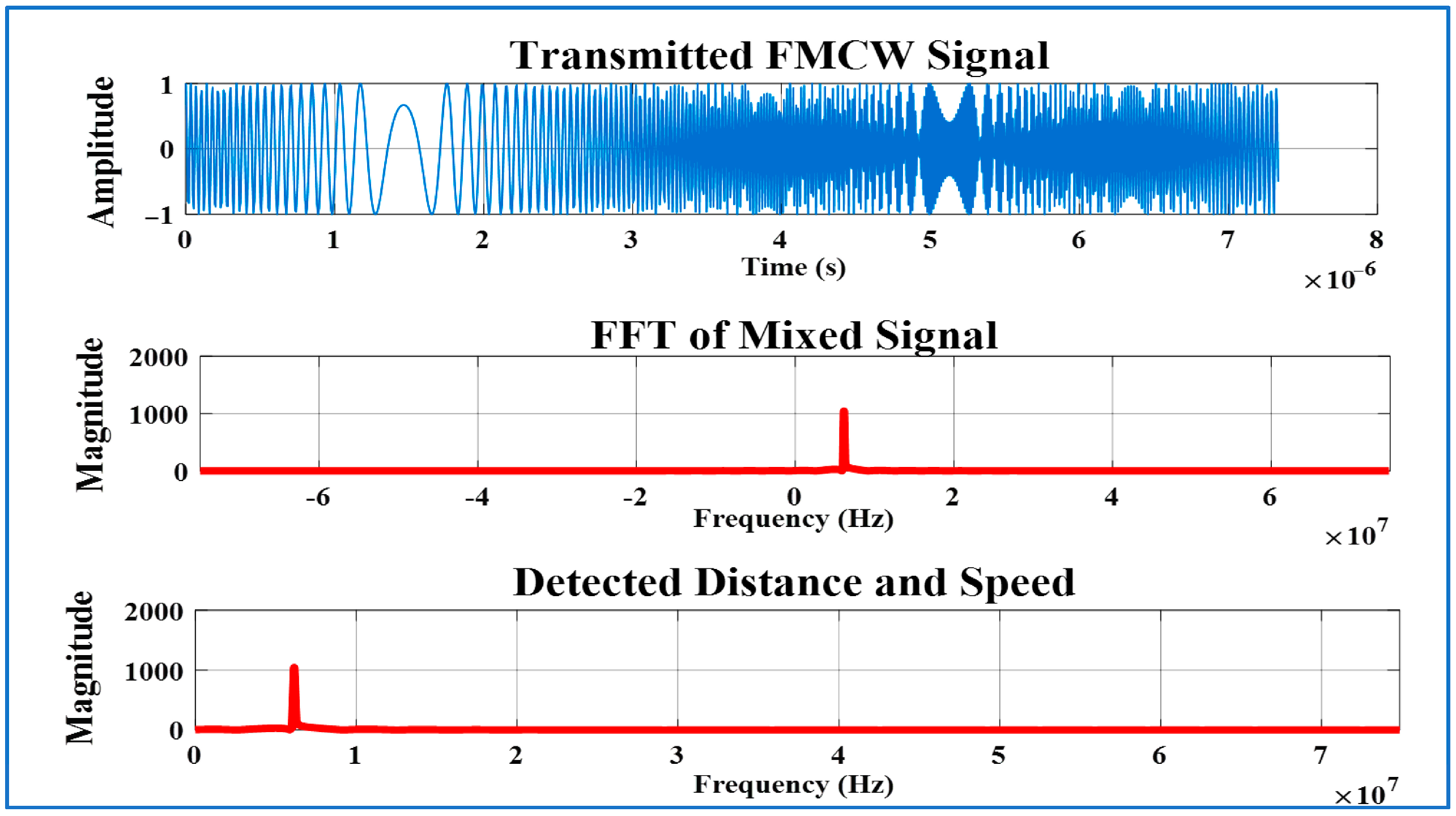
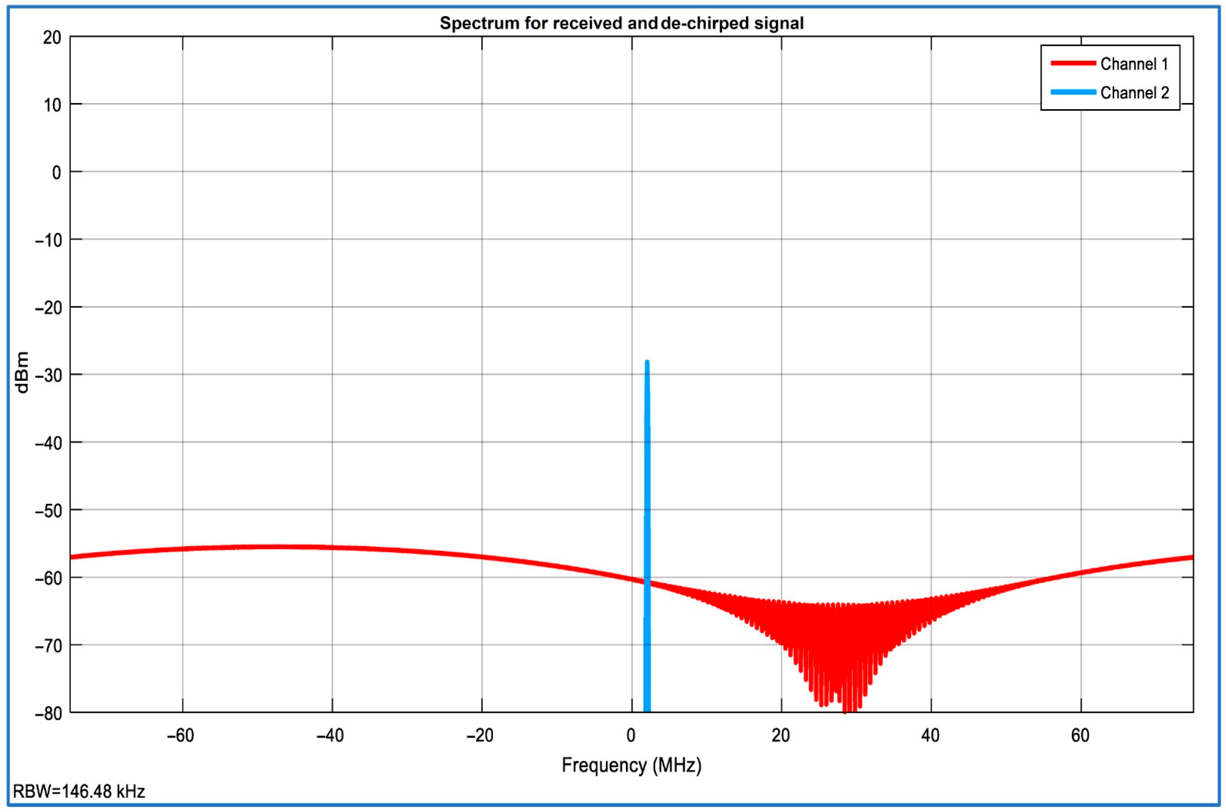
4.1.2. Signals of FMCW Radar

FMCW radar signals are essential for accurate distance and velocity measurements in automotive applications. Unlike traditional radar, FMCW continuously varies its frequency, using frequency shifts to calculate object distance and speed. This ensures high accuracy for automated stopping in autonomous vehicles. Figure 15 shows the following:

• Original FMCW Signal in Time Domain: Illustrates the signal’s amplitude evolution over time.
• Received FMCW Signal in Time Domain: Shows amplitude fluctuations after reflection from the target.
• De-chirped Signal: Displays the simplified signal for data analysis, enabling range and velocity extraction.
• FMCW Signal Spectrogram: Depicts energy distribution across frequencies over time, useful for identifying target features.

Figure 16 provides an overview of the key components and processes involved in FMCW radar signal analysis, showcasing the transmitted signal, signal processing steps, and detection outcomes. It illustrates each of the following:

• Transmitted FMCW Signal: Shows the frequency sweep of the signal, aiding in target recognition.
• FFT of Mixed Signal: Displays the Fast Fourier Transform (FFT) of the mixed signal, crucial for calculating target range and velocity.
• Detected Distance and Speed: Shows the plot of detected distance and speed using the beat frequency to calculate target range and speed.

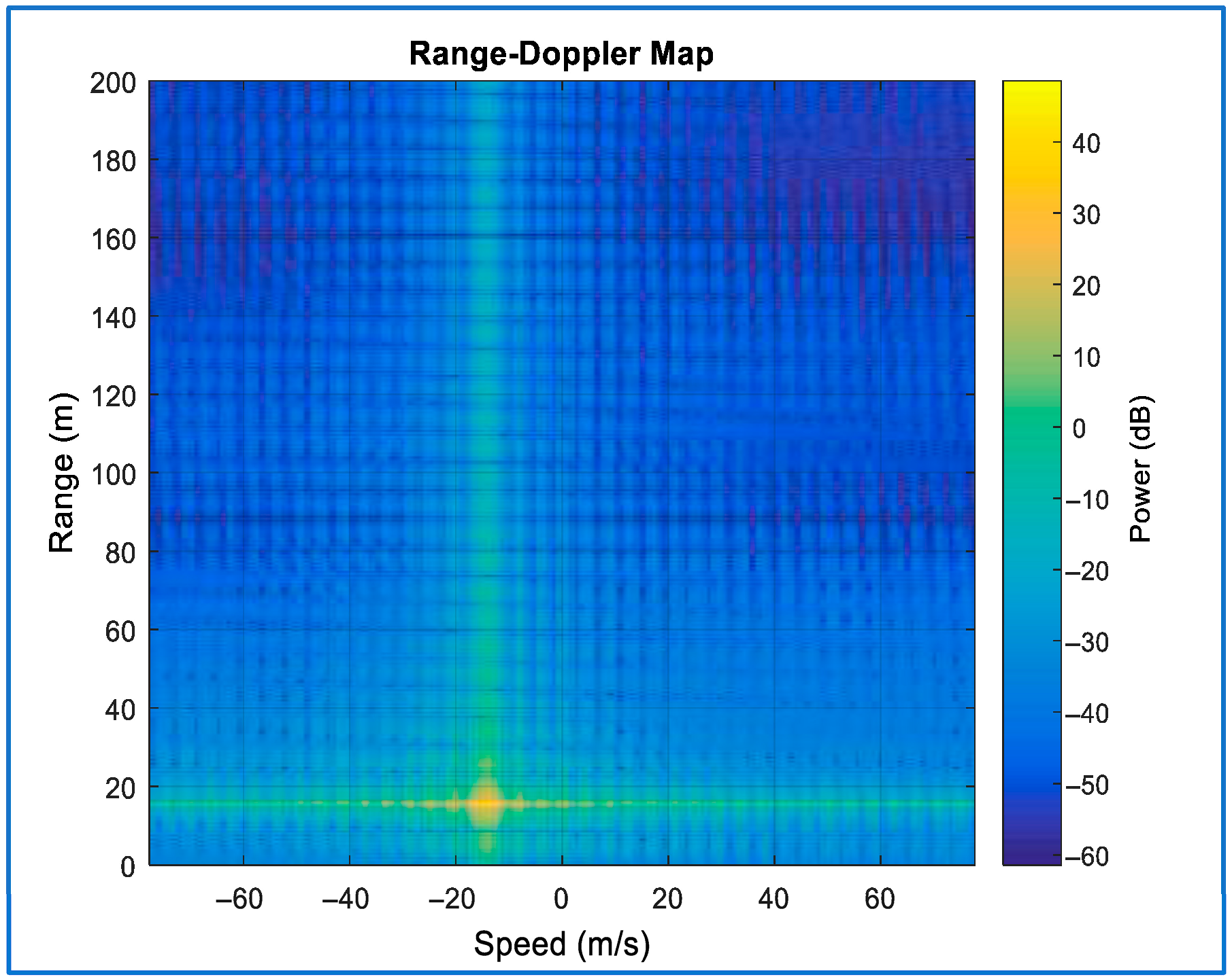
4.1.3. The Range-Doppler Map

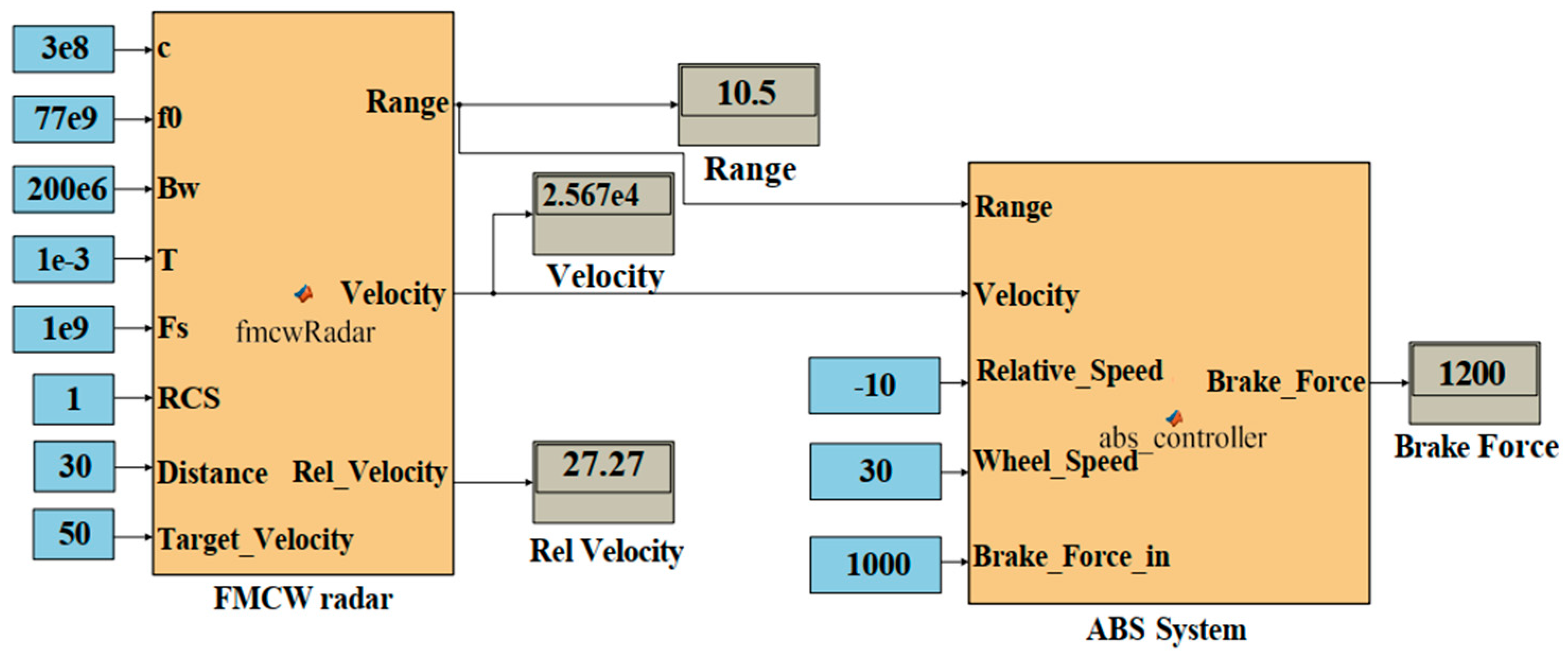
Figure 17 illustrates the Range-Doppler Map, which is used to estimate the range and relative velocity of targets. The horizontal axis represents velocity, while the vertical axis indicates range, aiding in determining the location and speed of multiple targets. Figure 18, on the other hand, demonstrates the influence of two-path propagation on the Range-Doppler Map, where this effect can cause interference and reduce the accuracy of range and velocity measurements.

Figure 19 shows the results of the three-way scan, which is used to obtain accurate range and velocity estimates by processing the up-sweep and down-sweep signals separately.

The vertical axis displays the signal power in decibels (dB), while the horizontal axis shows the frequency in megahertz (MHz). Red channel 1 shows a broad spectrum with a noticeable power dip at a range of approximately 15–45 MHz, suggesting potential interference or oscillations from the de-chirping operation. On the other hand, Channel 2, which is shown in blue, has a distinct peak at the 2 MHz frequency, indicating the existence of either a continuous wave signal with a fundamental frequency or a very low-frequency component.

4.2. ABSFMCW System

The ABSFMCW system enhances vehicle safety by integrating FMCW radar into braking systems. It accurately measures the distance and relative speed of nearby objects, enabling the system to adjust brake force and prevent wheel lock-up, ensuring stability, especially in difficult driving conditions.

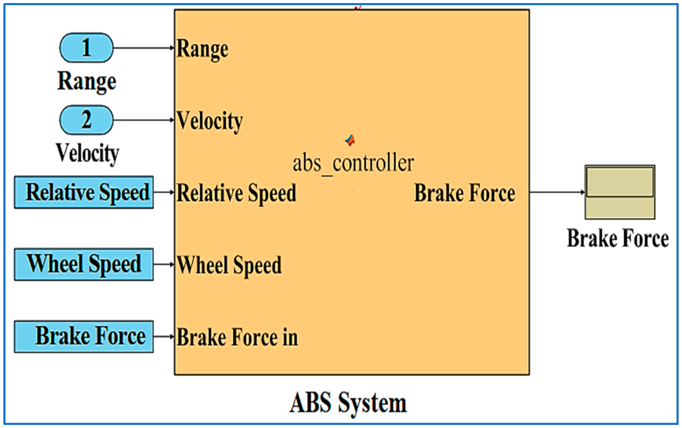
4.2.1. ABS Function Model

The ABS function model enhances vehicle safety by integrating ABS with FMCW radar, allowing real-time environmental monitoring for better adaptation to changing conditions. The system processes inputs like range, speed, wheel speed, and brake force to determine the necessary brake force, preventing wheel lock-up and maintaining stability during braking, as shown in Figure 20.

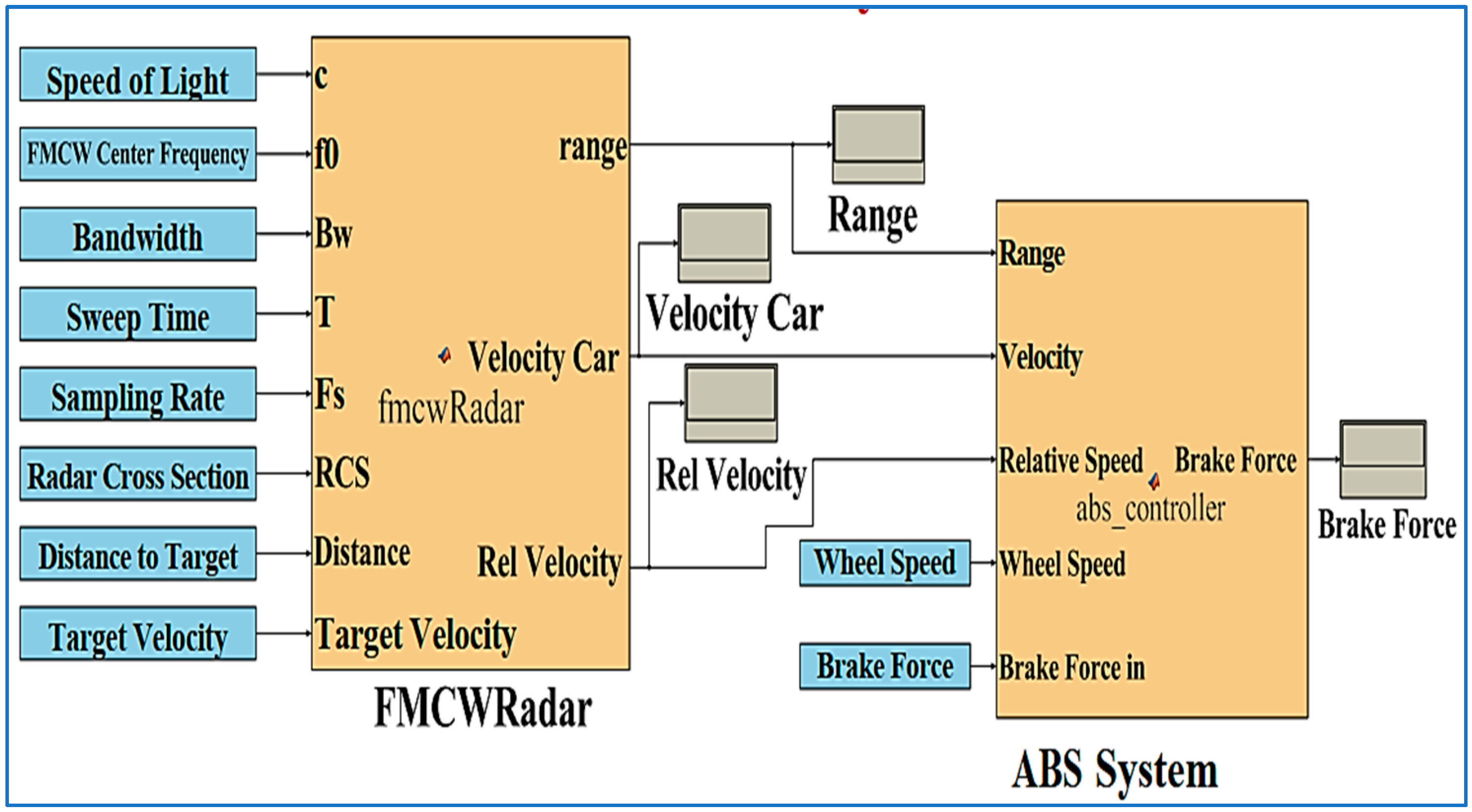
4.2.2. FMCW with ABS Function

The integrating of FMCW radar with ABS enhances braking performance by providing real-time data on vehicle speed, distance, and proximity to objects. The ABS dynamically adjusts braking force based on radar and vehicle data, ensuring optimal performance in various conditions and improving safety, especially in emergencies. Figure 21 illustrates the seamless data flow between radar, speed/wheel systems, and the braking force controller for responsive braking decisions. light blue is used for system parameters and input variables, such as speed of light, sweep time, and bandwidth; light orange highlights the two main subsystems the FMCW Radar and the ABS System helping to visually separate their roles; and gray is used for outputs like range, velocity, and brake force, indicating calculated or resulting values in the process flow.

A radar-based target detection system, illustrated in Figure 22, includes key components like the radar platform, signal processing modules, and FMCW radar. The system transmits signals via a TX Array and processes received echoes through modulation and reception steps. It calculates target speed and range, providing essential data for decision-making in applications like collision avoidance, surveillance, and autonomous vehicle navigation. light blue is used for key modules such as FMCW, Platform, and Car. Orange highlights the TX Array and RX Array components. Light red represents signal processing elements like Signal Processing and Free Space Channel. Purple is used for grouping larger system blocks such as RADAR and Channel and Target. Green boxes denote data transfer labels RadarPos, CarVel. Beige is used for output indicators like Range Estimate and Speed Estimate.

4.2.3. Programming of ABSFMCW

The programming of the ABS in combination with the FMCW radar is intended to permit smooth integration between the radar’s distance and speed readings and the braking control system. As demonstrated in Figure 23, the radar continually observes the vehicle’s surroundings, delivering real-time data concerning impediments and the relative speed of objects in the vehicle’s path. This information is processed by the ABS controller to adjust braking force, maintaining optimal wheel slip and preventing lock-up, thus enhancing safety and stability during automated stopping. Orange blocks represent core estimation units such as the RadarFMCW and ABS System modules, responsible for computing speed, range, and brake force. Yellow is used for the Controller Model, which generates control signals based on slip conditions. Light blue highlights dynamic subsystems such as the Friction Model and Wheel Model, which simulate physical and mechanical behaviors. Aqua-green is used for the slip computation logic, while beige boxes display key numeric inputs and outputs, such as range estimates, brake force, and wheel speed.

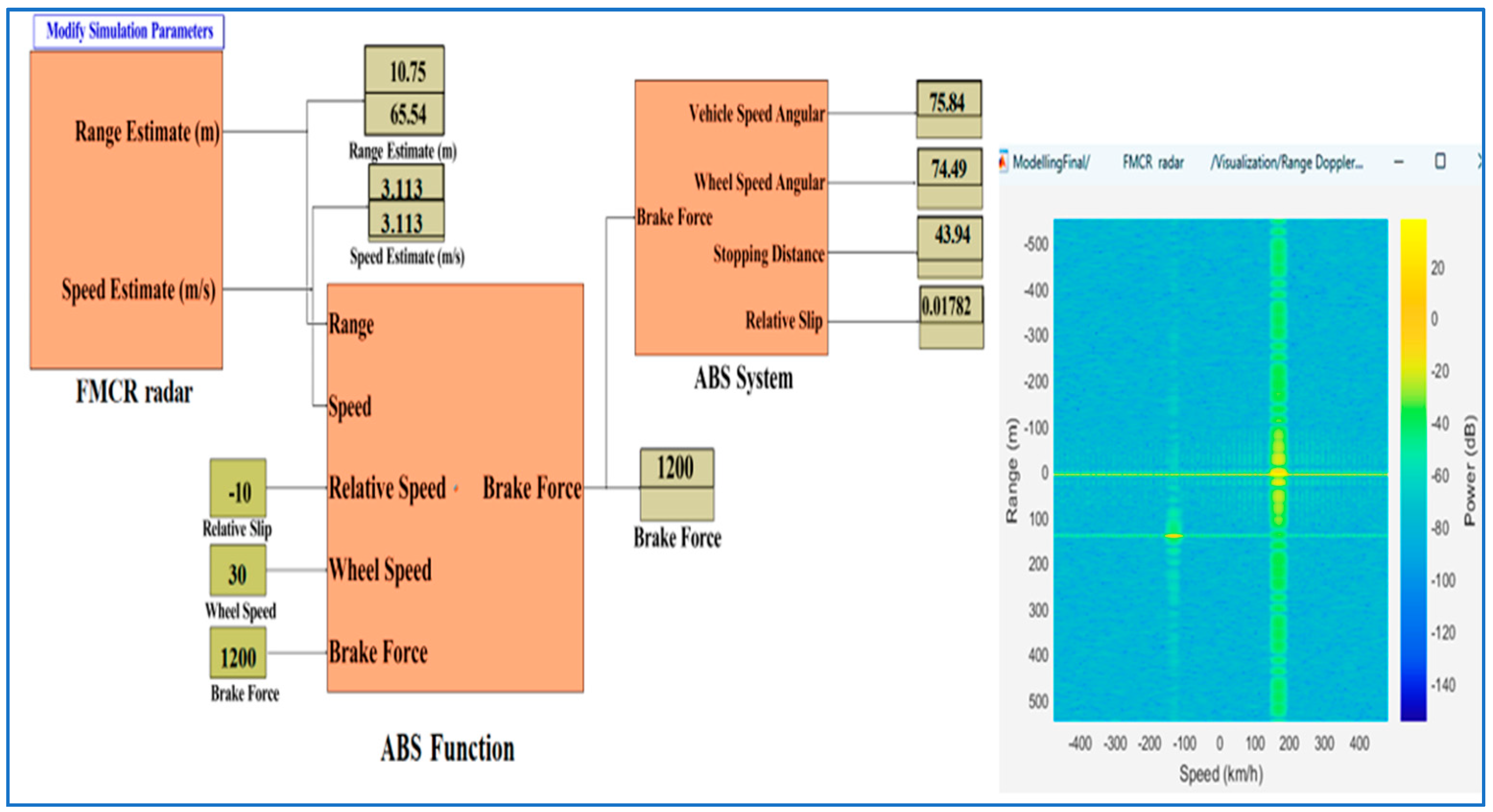
4.2.4. Simulation of ABSFMCW

Figure 24 illustrates the ABSFMCW radar model in MATLAB, showing the interaction between the radar system, which provides real-time data on distance and speed, and the ABS controller, which adjusts braking force based on this information. This setup allows the testing of the system under different conditions to ensure accurate obstacle response and effective wheel lock-up prevention, providing valuable insights for optimizing control strategies and improving safety in autonomous vehicles. The orange blocks represent the core processing systems FMCR radar and ABS System responsible for estimating vehicle dynamics and processing outputs like speed, range, and relative slip. The yellow block labeled ABS Function highlights the controller unit where inputs such as range, speed, and wheel data are processed to compute brake force. The light blue blocks denote input signal interfaces (e.g., Relative Speed, Wheel Speed, Brake Force), while the beige boxes indicate numerical outputs or parameter display modules.

4.2.5. Flowchart of Automatic Braking System Using FMCW Radar

The flowchart in Figure 25 demonstrates the working of an autonomous braking system that employs FMCW radar to analyze distances and activate the ABS upon detecting a probable impediment within a defined range. The process starts with the activation of the radar system, followed by the ongoing collecting and updating of distance data. The evaluated distance is compared with a set threshold. Should the distance shrink inside this threshold, the ABS is engaged, initiating the braking action. The technology assesses the efficiency of the braking action prior to deactivating the radar system, therefore providing a controlled and secure response to potential collision circumstances. The green color at the top marks the start of the process, while the orange at the bottom indicates the end. The light blue rectangles represent standard operational or processing steps, such as reading data or performing braking. The peach-colored diamonds denote decision points, where conditions are evaluated to determine the flow direction. The purple arrows indicate the logical flow from one step to the next.

4.2.6. Working Principle of Radar and System Integration

FMCW radar generates a continuous, frequency-modulated signal that reflects off surrounding objects, enabling precise real-time measurements of distance and relative velocity. When integrated with a hybrid PID-FLC control system, the radar continuously monitors the environment, detecting obstacles and other vehicles. This integration enables the brake system to make quick and exact changes to braking force, guaranteeing smooth and efficient stopping even under fluctuating road and traffic situations. The radar’s capacity to detect changes in the surroundings in real-time, combined with the adaptive control methods of the PID and FLC, increases the vehicle’s overall responsiveness and safety. This section looks into the operating mechanics of the FMCW radar, the process of integrating it with the hybrid controller, and how these components interact synergistically to provide dependable, accurate, and timely automated stopping.

5. Results of Simulation

The simulation results are crucial for evaluating the effectiveness of the proposed control system for autonomous vehicle stopping, utilizing ABS and FMCW radar technology. The simulation aims to assess the system’s performance across various scenarios, including changes in environment, vehicle speeds, and stopping patterns. By analyzing the results, the accuracy and effectiveness of the system in enhancing vehicle safety and providing quick, precise responses to stopping needs can be determined.

5.1. Range and Velocity

The self-operating ABS employing FMCW radar depends on range and velocity measurements because they allow exact regulation of the braking power to ensure safe and effective vehicle stopping as well as accurate obstacle identification. Figure 26 depicts the range between the vehicle and the target, as well as the target speed, when the ABS is automatically engaged. The orange blocks represent the core functional systems; the FMCW Radar and the ABS System. The light blue blocks indicate system parameters or constants used for simulation inputs (e.g., speed of light, frequency, and time intervals), while the beige blocks display the computed outputs such as range, velocity, and brake force.

Figure 27 indicates the distance between the automobile and the target as well as the target speed, when the ABS is automatically engaged, as depicted in the photo. The orange blocks represent core functional subsystems, including the FMCR radar, ABS Function, and ABS System, which are responsible for processing inputs and producing outputs. The blue block labeled "Modify Simulation Parameters" highlights the simulation input configuration interface. Meanwhile, the beige blocks are used to present numerical output values such as range, speed, and braking force.

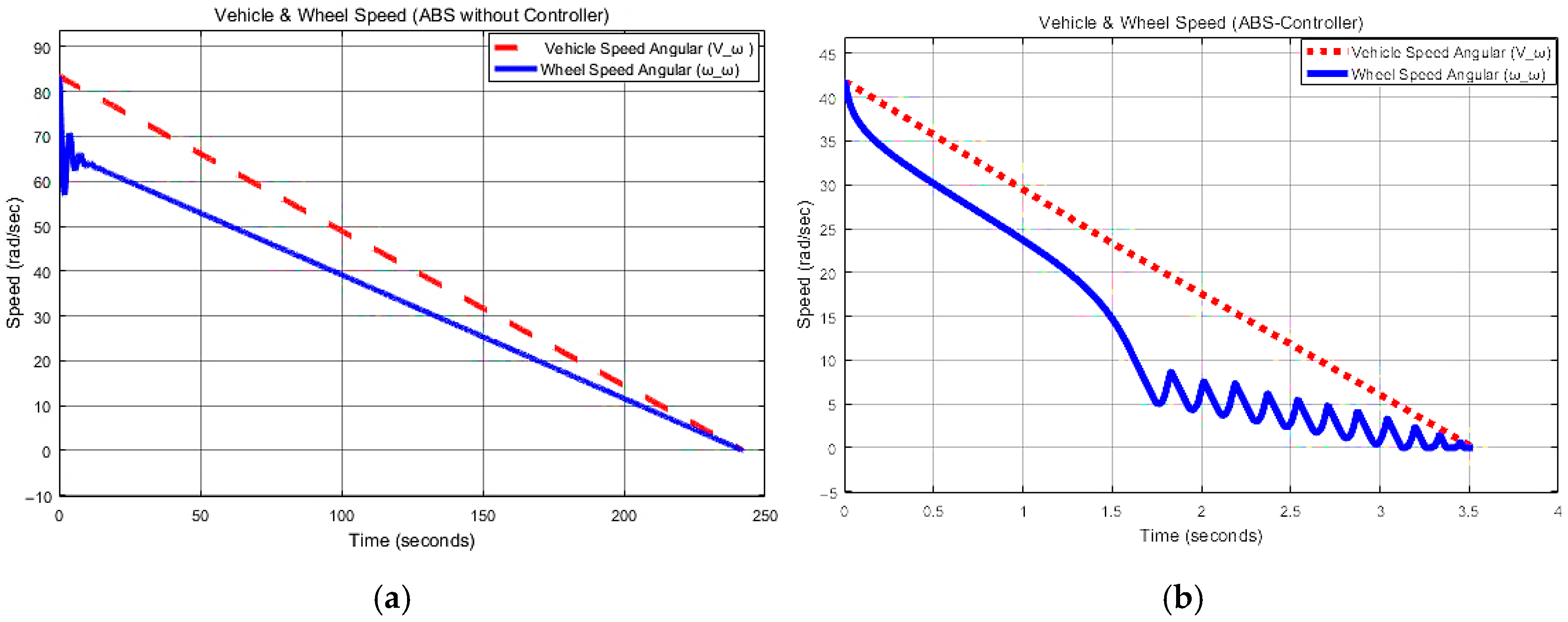
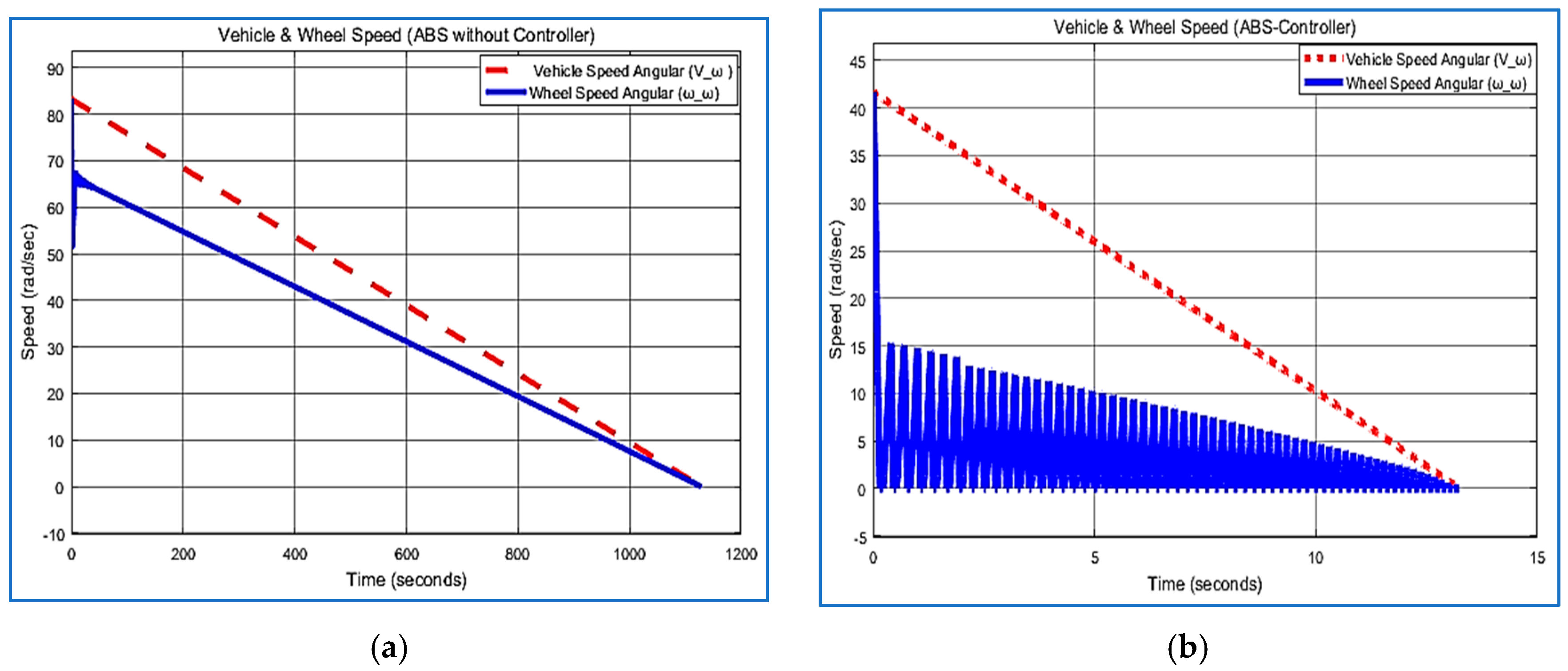
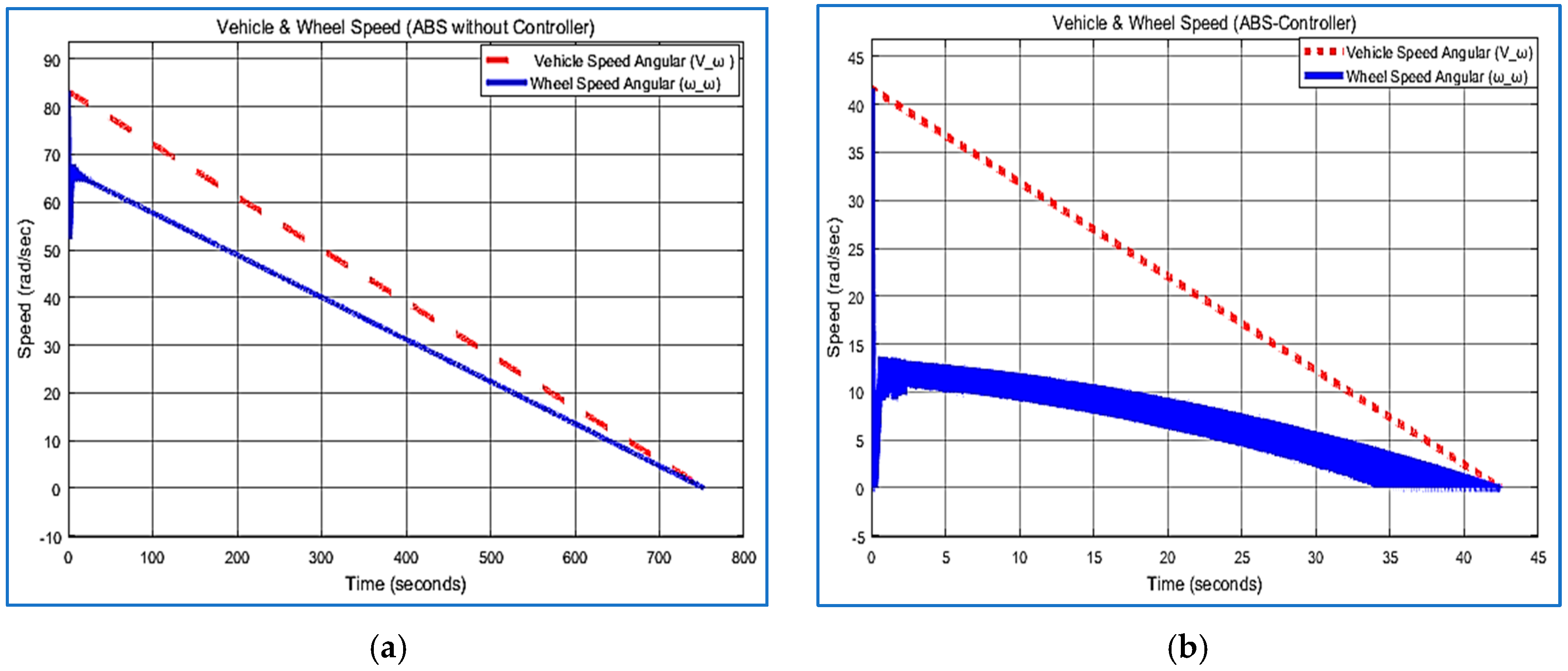
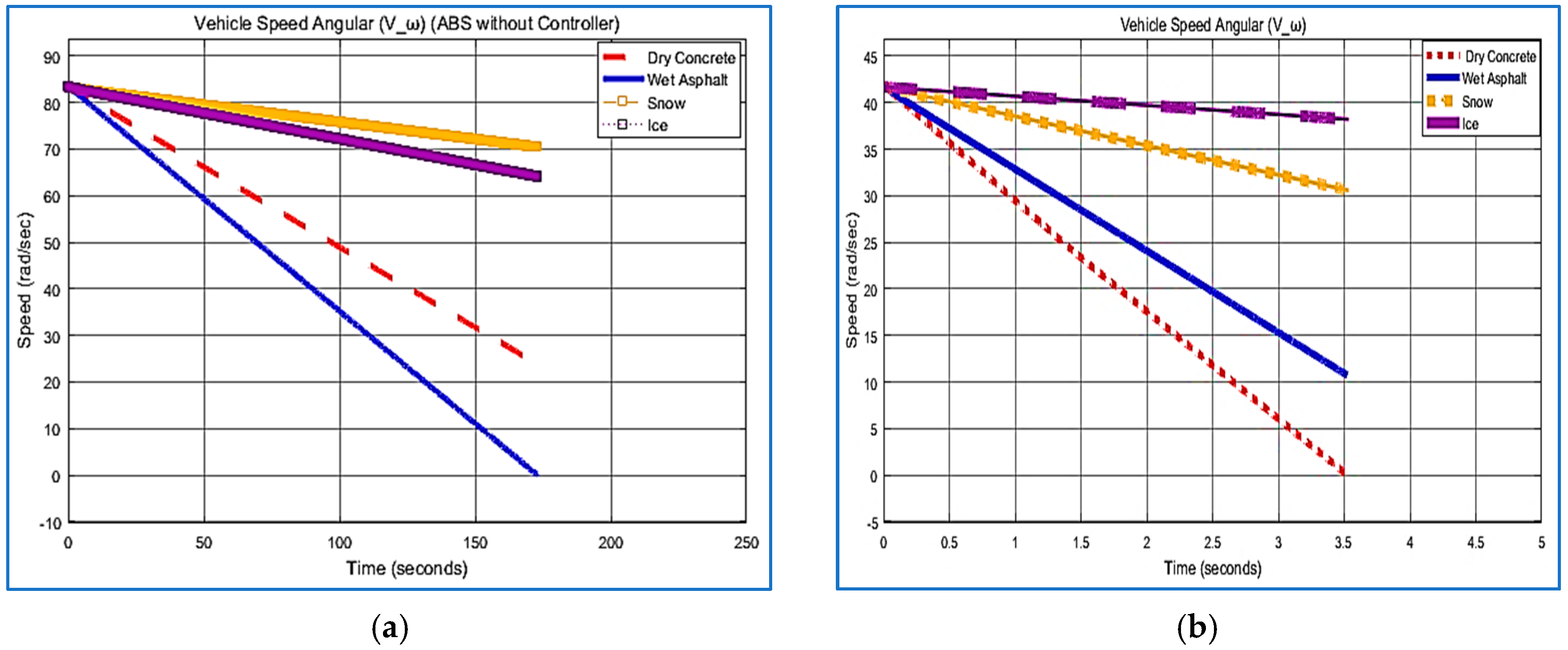
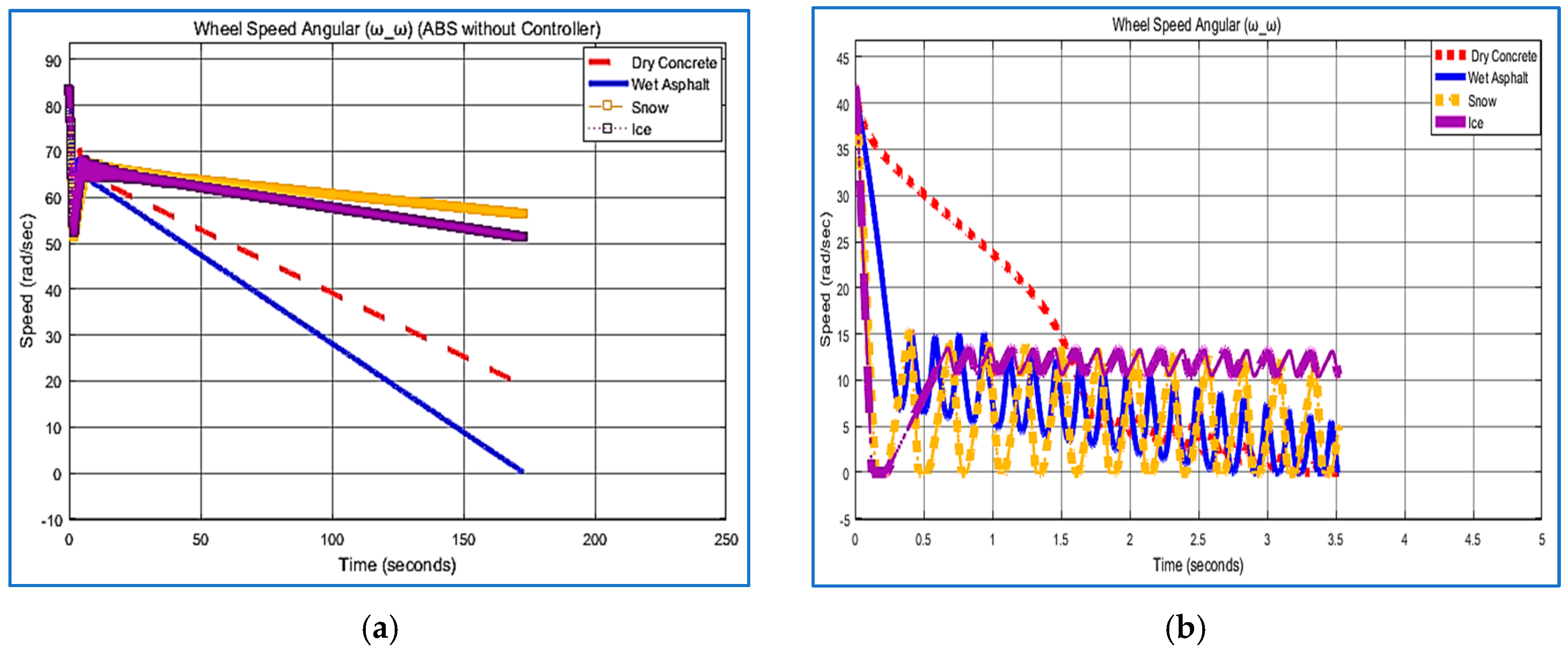
5.2. Vehicle and Wheel Speed

Figure 28 shows vehicle and wheel speeds on dry concrete during two braking scenarios. Figure 28a illustrates braking without a controller unit for the ABS, causing a sharp decline in wheel angular speed that results in wheel lock-up and loss of control. In contrast, Figure 28b shows braking with the controller unit, which optimally modulates brake force to prevent lock-up, thereby maintaining wheel speed and enhancing control and stability on dry surfaces. This dynamic adjustment improves safety by ensuring better traction during braking.

Figure 29 shows vehicle and wheel speeds on wet asphalt in two braking scenarios. In Figure 29a, without a controller unit for the ABS, the wheels lock quickly due to reduced friction, leading to a sharp decline in wheel angular velocity. Figure 29b shows braking with the controller unit, maintaining traction and minimizing wheel lock-up, resulting in prolonged oscillations in wheel angular velocity as the system balances braking force and control.

Figure 30 illustrates vehicle and wheel speeds on a snowy road during braking in two scenarios. In Figure 30a, without a controller unit for the ABS, the wheels lock quickly, causing a significant mismatch between wheel angular speed and vehicle speed, leading to reduced grip and higher risk of skidding. In Figure 30b, with a controller unit for the ABS, the system modulates brake pressure to prevent lock-up, resulting in broader and less constant oscillations in wheel speed, which improves grip and enhances braking control on the snowy surface.

Figure 31 compares vehicle and wheel speed behavior on an icy road during braking under two conditions: without and with an ABS control unit. In Figure 31a, without the ABS, the wheels lock quickly, causing a rapid loss of traction and control, increasing the risk of sliding. In contrast, Figure 31b shows the ABS control unit adjusting brake force to prevent wheel lock-up, allowing for a more gradual and controlled deceleration, helping the driver maintain control in slippery conditions.

Simulation curves show that dry concrete provides better control and faster stopping due to higher friction. Wet pavement reduces stability, increasing wheel slip and braking distance. Snowy roads cause slower speeds and more wheel slip, making control harder, while icy roads create the most difficult conditions, with significant tire slippage and longer stopping distances.

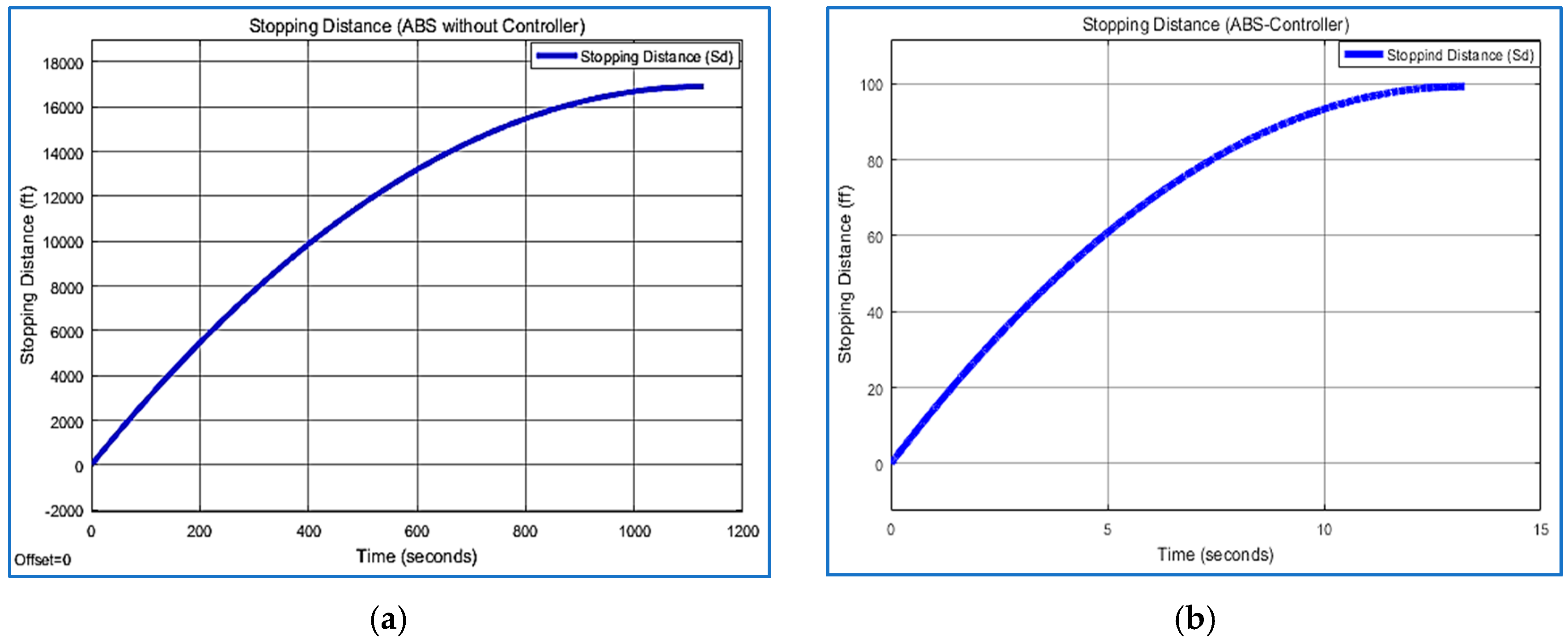
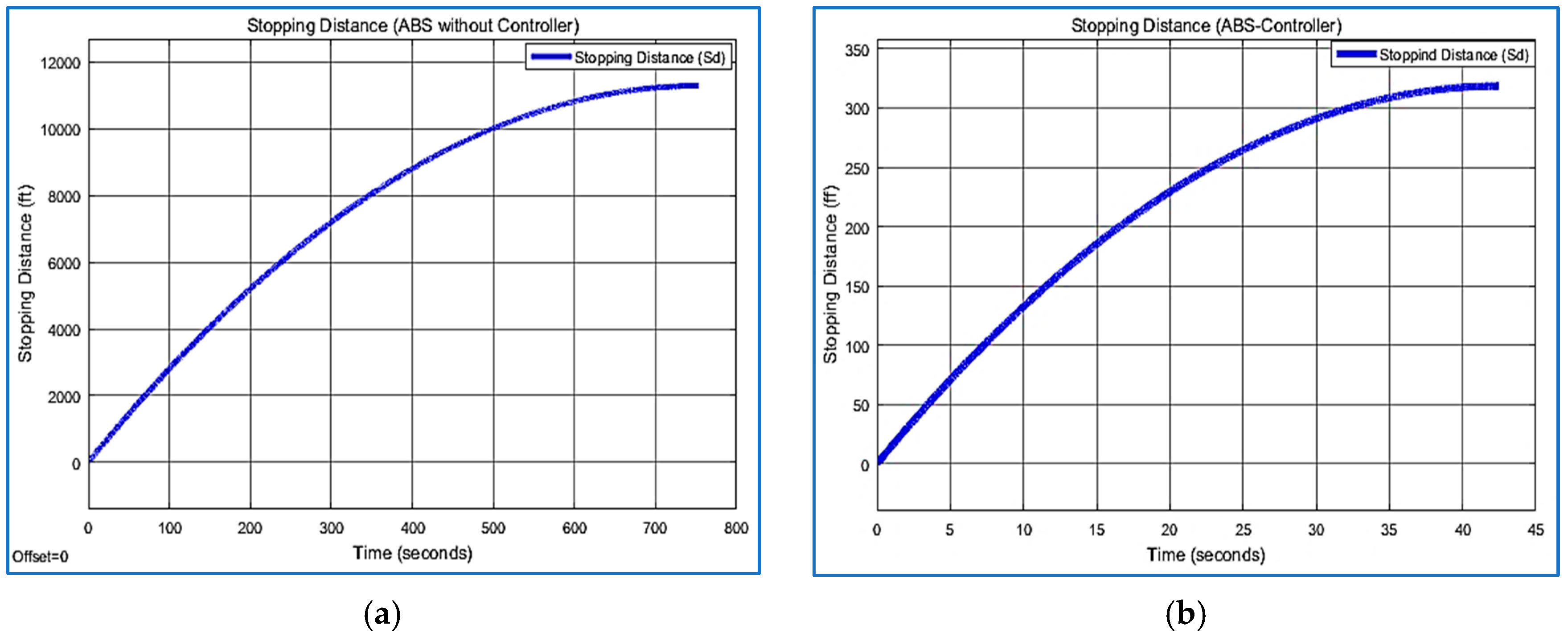
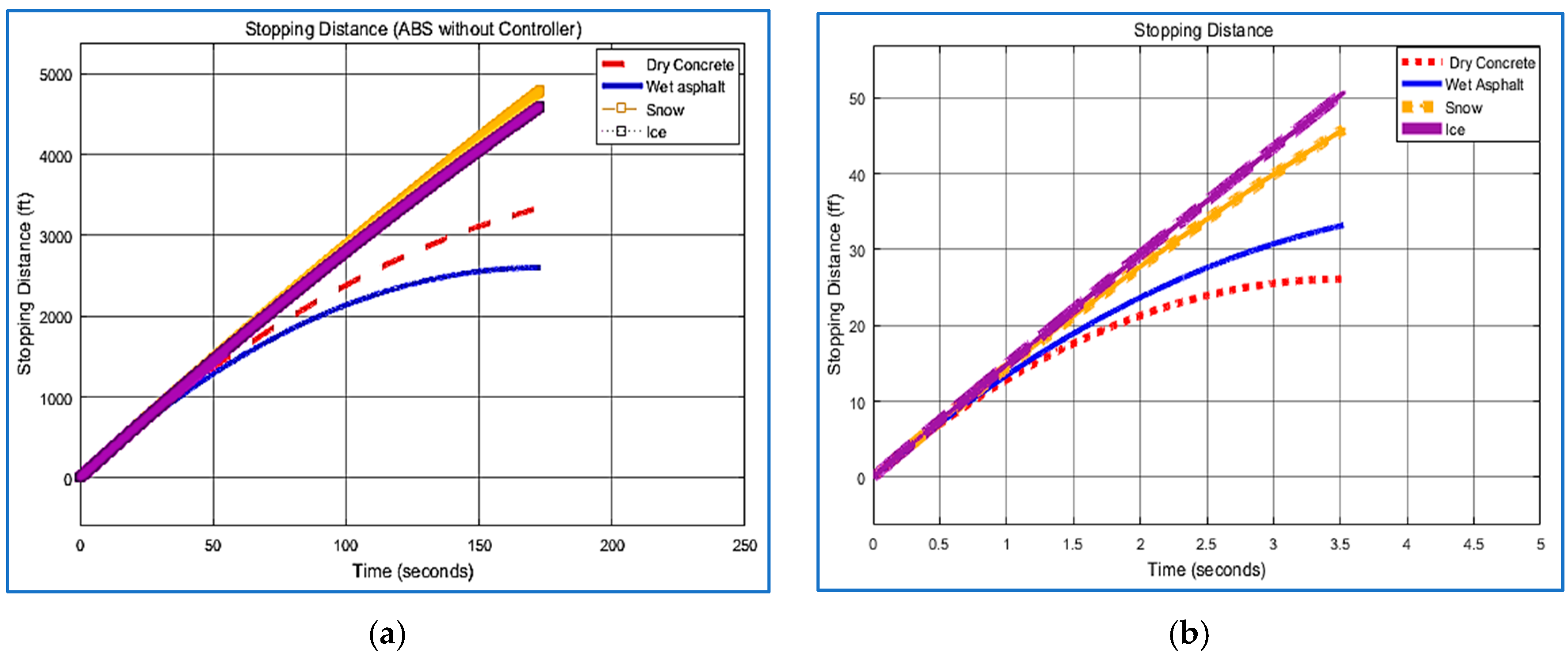
5.3. Stopping Distance

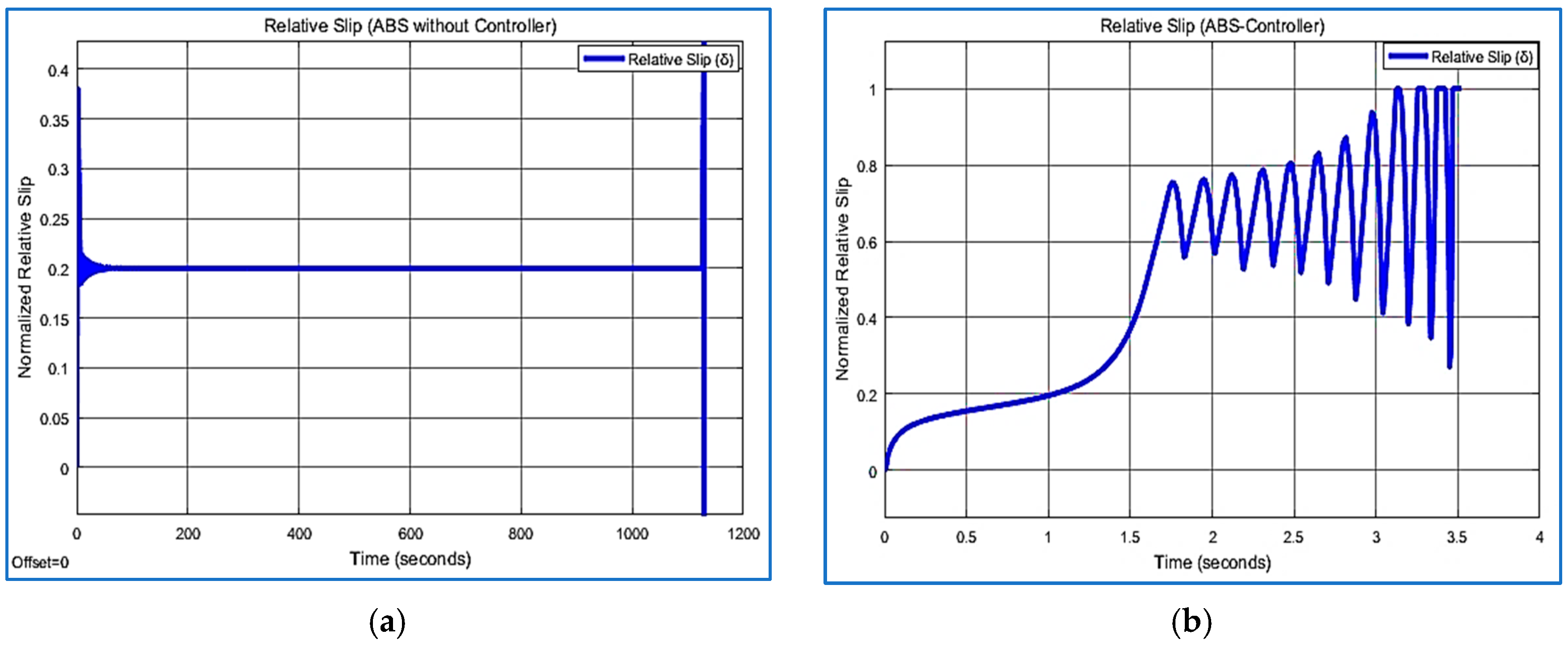
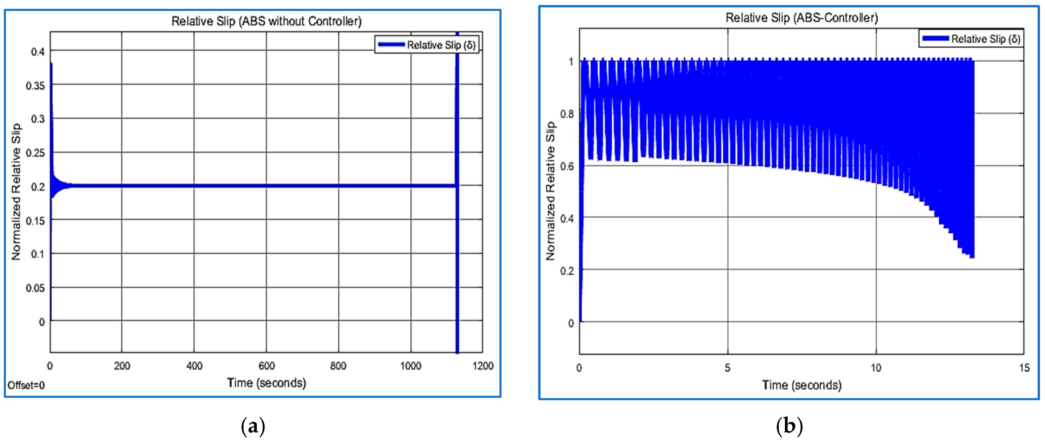
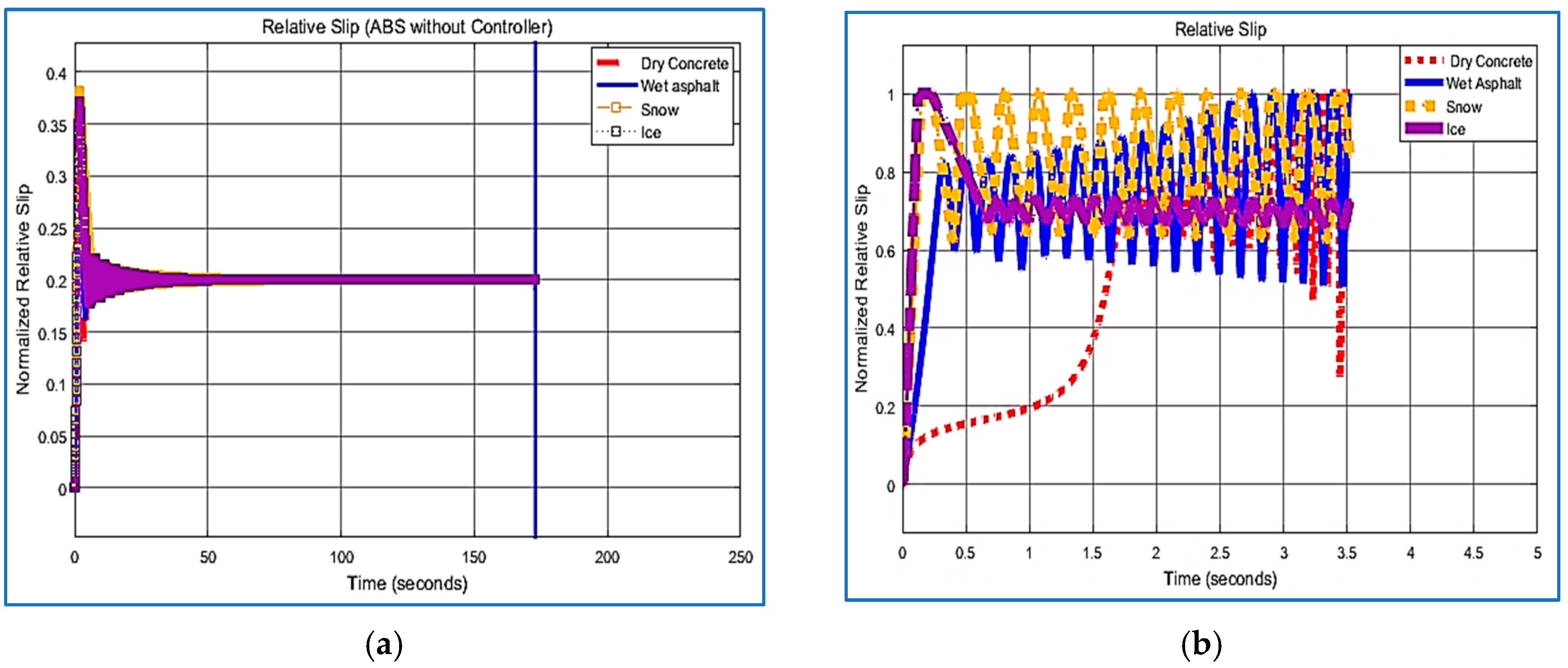
Figure 32 shows stopping distance on dry concrete with and without the controller unit in the ABS. In Figure 32a, without the controller, the stopping distance is longer due to uncontrolled wheel slip, reducing traction and braking efficiency. In contrast, Figure 32b demonstrates that with the controller, the system optimizes wheel slip, improving traction and significantly shortening the stopping distance, highlighting the importance of the ABS for enhanced braking performance and safety.

Figure 33 compares stopping distance on wet asphalt with and without the activation of the controller unit in the ABS. In Figure 33a, without the controller, reduced tire–road friction increases stopping distance due to uncontrolled wheel slip, leading to longer braking. In Figure 33b, with the controller, the system adjusts braking forces to maintain optimal slip ratios, improving traction and stability, resulting in a significant reduction in stopping distance even on low-friction surfaces.

Figure 34 demonstrates the ABS controller’s effect on stopping distances on snow-covered roads. In Figure 34a, without the controller, the low friction leads to frequent wheel lockups, extending stopping distances and compromising vehicle control. Conversely, Figure 34b shows that with the ABS activated, the system adjusts braking force to prevent wheel lockup, improve traction, maintain stability, and significantly shorten stopping distances in snowy conditions.

Figure 35 compares stopping distances on an icy road with and without a control unit in the ABS. In Figure 35a, without the control unit, wheel lockup and reduced traction cause a significant increase in stopping distance. In Figure 35b, the control unit optimizes wheel slip, preventing lockup, and enhancing traction. This dynamic brake pressure adjustment allows for better control and a substantial reduction in stopping distance on low-friction surfaces like ice.

The stopping distance of a vehicle varies substantially according to road conditions. On dry concrete, it is negligible, indicating good ABS functioning. It increases on wet asphalt due to reduced friction, requiring more time to brake. Snowy roads increase stopping distance due to a significant reduction in friction, making safe stopping more difficult. The longest stopping distance occurs on ice roads, when minimal friction causes significant loss of control and a longer stopping distance.

5.4. Relative Slip

Figure 36 depicts the influence of the controller unit in Anti-ABS on the relative slip of tires when braking on a dry concrete road. In Figure 36a, when braking occurs without a controller unit, the relative slip stays practically constant at a low level, showing little and consistent tire slide. Conversely, as shown in Figure 36b, when a controller unit is operating, the relative slip changes fast between high and low values. This rhythmic motion demonstrates the efficiency of a controller unit in avoiding wheel lockup by continually altering braking pressure, hence boosting vehicle stability and control.

Figure 37 illustrates the stopping distance of a vehicle on an icy road under two scenarios: Figure 37a shows the results without a control unit in the ABS and Figure 37b shows the results with a control unit in the ABS. Figure 37a shows wheel lockup and reduced traction leading to increased stopping distances. However, Figure 37b shows more controlled stopping behavior, highlighting the ABS control unit’s effectiveness in maintaining optimal wheel slip and preventing lockup. By continuously regulating brake pressure, the ABS unit enhances traction and maintains steering control, reducing stopping distances on low-friction surfaces like ice.

Figure 38 compares tire relative slip on a snowy road with and without a controller unit in the ABS. In Figure 38a, without the controller, the relative slip remains low but stable, indicating gradual loss of tire-road adhesion and reduced vehicle control. In contrast, Figure 38b shows rapid fluctuations in relative slip with the controller, as the system adjusts brake force to prevent wheel lockup. Despite the oscillations, the average relative slip is lower than without the controller, demonstrating improved traction and better vehicle control on snowy surfaces.

Figure 39 compares tire relative slip on an ice road with and without a controller unit in the ABS. In Figure 39a, without the controller, the relative slip remains low and steady, indicating minimal tire slide but a gradual loss of tire–road adhesion, reducing vehicle control. In Figure 39b, with the controller, the relative slip fluctuates significantly as the system engages and disengages the brakes to prevent wheel lockup. Despite these fluctuations, the average relative slip is lower than without the controller, suggesting better traction and improved vehicle control on icy surfaces.

The sliding rate varies with road conditions. Dry concrete has the lowest sliding rate, providing excellent control and ABS efficiency in preventing wheel slide. Wet asphalt increases the sliding rate due to reduced friction, making stopping harder. Snowy roads further challenge vehicle stability with a higher sliding rate, while icy roads present the most difficulty, with a very high sliding rate leading to severe skidding and significant loss of control.

5.5. Limitations and Future Work

While simulation-based validation offers valuable insights, it cannot fully replicate real-world sensor noise, actuator latency, or environmental uncertainty. As recommended by Gao et al. [35] and Zhou et al. [36], future work will include hardware-in-the-loop simulation and field testing to verify the controller’s robustness under real-world conditions.

6. Discussion of Results

This study investigated the integration of FMCW radar technology with ABS braking systems to improve the stopping performance of autonomous vehicles. The findings indicated enhanced stopping accuracy and reduced stopping distances, particularly under adverse road conditions such as wet or slippery surfaces, where the radar system effectively detected obstacles and adjusted braking force accordingly. Moreover, the integration of radar technology contributed to improved vehicle stability by dynamically modulating braking force, thereby preventing wheel lock-up and enhancing control during emergency stops. Although the simulation results were promising, the study emphasizes the need for further research to develop advanced control algorithms and optimize the interaction between the radar and braking systems. It is recommended that future studies focus on real-world testing to validate and refine the system’s performance in diverse driving environments. The final part of the discussion presents figures that compile simulations under various conditions, illustrating the impact of the control unit within the ABS on vehicle acceleration during braking across different road surfaces. These figures provide valuable insights into how the control unit influences vehicle dynamics in diverse scenarios.

Figure 40 compares vehicle angular speed during braking on different road surfaces with and without the controller unit in the ABS. In Figure 40a, angular velocity decreases steadily, leading to longer stopping times. In Figure 40b, the controller modulates brake pressure, reducing stopping time and improving stability, particularly on low-friction surfaces.

Figure 41 illustrates the effect of the controller unit in the ABS on wheel angular speed during braking across different surfaces. In Figure 41a, without the controller, angular velocity decreases linearly, risking lockup and loss of control. In Figure 41b, the controller modulates brake pressure, improving efficiency, reducing stopping time, and enhancing stability.

Figure 42 depicts the influence of the controller unit in the ABS on vehicle stopping distance across different road conditions. In Figure 42a, longer stopping distances occur due to wheel lockup. In Figure 42b, the controller reduces stopping distances by adjusting brake pressure, improving braking efficiency and stability.

Figure 43 demonstrates the influence of the controller unit in the ABS on tire relative slip during braking. In Figure 43a, excessive slip occurs without the controller, reducing efficiency and stability. In Figure 43b, the controller maintains optimal slip, enhancing braking, handling, stability, and safety.

The ramifications of halting distance and duration under various conditions are shown in

Table 4. Stopping time and distance without ABS-Controller.

	Road Type	Dry Concrete	Wet Asphalt	Snow	Ice
Cases
Stopping Time (s) with ABS-Controller		3.522	4.743	13.240	42.442
Stopping Distance with ABS-Controller (ft)		26.12	35.55	99.35	318.51
Stopping Distance with ABS-Controller (m)		7.96	10.33	30.28	97.08
Stopping Time (s) without ABS-Controller		242.106	172.979	1128.494	753.033
Stopping Distance without ABS-Controller (ft)		3635	2600	16,900	11,280
Stopping Distance without ABS-Controller (m)		1107.95	792.48	4876.80	3438.14

.

The data in the table highlights a significant increase in stopping distance and time when driving on ice roads compared with dry ones, indicating that the performance and effectiveness of the ABS are highly influenced by the friction coefficient. The ABS and vehicle performance are significantly impacted by the type and condition of the road, with dry roads yielding the best performance and icy roads presenting the most challenges. This study emphasizes the importance of improving vehicle control systems to enhance safety in various driving conditions.

6.1. Advanced Braking Systems

The proposed braking architecture draws inspiration from recent EMB designs, which demonstrate high performance in distributed control environments. As highlighted by Wu et al. [3], optimization of EMB parameters via multi-objective design contributes significantly to safety and comfort. In our model, braking response time and smoothness are evaluated against EMB benchmarks, showing comparable or superior performance in mid- and low-friction scenarios.

6.2. FMCW Technique with ABS

Figure 44 displays a Doppler map generated by a FMCW radar system, commonly used in military, industrial, and automotive applications. This map shows the relationship between target range (horizontal axis), relative velocity (vertical axis), and signal strength (reflected signal power). Stronger signals are represented by brighter colors. Targets within the radar’s field of view reflect part of the radar’s transmitted signal. The Doppler frequency, linked to the relative velocity of the target, is determined by comparing transmitted and reflected signals. A Fourier transform is applied to the received signal, generating a frequency spectrum. This map helps assess the target’s speed and distance, particularly when the ABS is automatically triggered. The orange blocks indicate key functional components, including the FMCR radar, ABS function, and ABS system modules. These modules work together to process range and speed estimates, determine wheel and vehicle dynamics, and apply braking force accordingly. The yellow panels display simulation outputs such as range estimate, speed, wheel speed, relative slip, brake force, and stopping distance in real-time. The blue section on the right illustrates the Range-Doppler visualization, showing radar detection results.

7. Conclusions

This research focused on developing an integrated control system for autonomous vehicle braking by combining FMCW radar technology with an ABS. The proposed system employs a hybrid control strategy, integrating FLC and PID controllers to optimize braking performance, vehicle stability, and safety in emergency scenarios and diverse driving conditions. Simulations were conducted under various road conditions, including dry, wet, snowy, and icy surfaces, as well as varying traffic congestion. Results demonstrated significant improvements in stopping distance, response time, and stability compared with systems without ABS. These improvements were attributed to the dynamic adjustment of braking force based on high-resolution range and velocity data provided by FMCW radar. The system efficiently modulated wheel slip and maintained optimal traction, even under low-friction conditions. This research highlights the potential of integrating advanced radar technology and control algorithms to enhance the safety and reliability of autonomous vehicle braking systems, setting a foundation for future advancements in autonomous driving technologies. Although the results are validated through simulation, real-world testing and hardware-in-the-loop validation are recognized as essential next steps. Future work will focus on implementing the controller in experimental platforms to evaluate performance under dynamic, multi-target, and interference-prone environments. The literature review is expanded to reflect the broader urban, regulatory, and human-factor dimensions of autonomous braking systems.

References

1. Zhou, Z.; Rother, C.; Chen, J. Event-Triggered Model Predictive Control for Autonomous Vehicle Path Tracking: Validation Using CARLA Simulator. IEEE Trans. Intell. Veh. 2023, 8, 3547–3555. [Google Scholar] [CrossRef]
2. Zhu, Z.; Pivaro, N.; Gupta, S.; Gupta, A.; Canova, M. Safe Model-Based Off-Policy Reinforcement Learning for Eco-Driving in Connected and Automated Hybrid Electric Vehicles. IEEE Trans. Intell. Veh. 2022, 7, 387–398. [Google Scholar] [CrossRef]
3. Wu, T.; Li, J.; Qin, X. Braking performance oriented multi–objective optimal design of electro–mechanical brake parameters. PLoS ONE 2021, 16, e0251714. [Google Scholar] [CrossRef] [PubMed]
4. Cao, D.; Wang, X.; Li, L.; Lv, C.; Na, X.; Xing, Y.; Li, X.; Li, Y.; Chen, Y.; Wang, F. Future Directions of Intelligent Vehicles: Potentials, Possibilities, and Perspectives. IEEE Trans. Intell. Veh. 2022, 7, 7–10. [Google Scholar] [CrossRef]
5. Gao, F.; Han, Y.; Li, S.E.; Xu, S.; Dang, D. Accurate Pseudospectral Optimization of Nonlinear Model Predictive Control for High-Performance Motion Planning. IEEE Trans. Intell. Veh. 2023, 8, 1034–1045. [Google Scholar] [CrossRef]
6. Moloto, R.; Nyandoro, O.T.C. Review of Wheel Slip Control Design Strategies for Vehicular Anti-Lock Braking Systems; University of the Witwatersrand: Johannesburg, South Africa, 2024; Available online: https://www.researchgate.net/publication/382495607_Review_of_Wheel_Slip_Control_Design_Strategies_for_Vehicular_Anti-Lock_Braking_Systems (accessed on 10 July 2025).
7. El-Bakkouri, J.; Ouadi, H.; Giri, F.; Khafallah, M.; Gheouany, S.; El Bakali, S. Extremum Seeking Based Braking Torque Distribution for Electric Vehicles’ Hybrid Anti-Lock Braking System. IFAC-PapersOnLine 2023, 56, 2546–2551. [Google Scholar] [CrossRef]
8. Pérez, J.; Alcázar, M.; Sánchez, I.; Cabrera, J.A.; Nybacka, M.; Castillo, J.J. On-line learning applied to spiking neural network for antilock braking systems. Neurocomputing 2023, 559, 126784. [Google Scholar] [CrossRef]
9. Chen, H.C.; Wisnujati, A.; Widodo, A.M.; Song, Y.L.; Lung, C.W. Antilock Braking System (ABS) Based Control Type Regulator Implemented by Neural Network in Various Road Conditions; Springer International Publishing: Cham, Switzerland, 2022; Volume 313. [Google Scholar] [CrossRef]
10. Al-Mola, M.H.A.; Mailah, M.; Salim, M.A. Applying Active Force Control with Fuzzy Self-Tuning PID to Improve the Performance of an Antilock Braking System. Int. J. Nanoelectron. Mater. 2021, 14, 489–502. [Google Scholar]
11. Haris, I.; Ahmad, F.; Hassan, M.H.C.; Yamin, A.K.M.; Nuri, N.R.M. Self Tuning PID Control of Antilock Braking System using Electronic Wedge Brake. Int. J. Automot. Mech. Eng. 2021, 18, 9333–9348. [Google Scholar] [CrossRef]
12. Reitz, P.; Künzle, C. Evaluation of the Interference Performance of FMCW Radar Sensors in Dense Indoor Environments. IEEE Access 2024, 12, 46834–46850. [Google Scholar] [CrossRef]
13. Guo, M.; Zhao, D.; Wu, Q.; Wu, J.; Li, D.; Zhang, P. An Integrated Real-Time FMCW Radar Baseband Processor in 40-nm CMOS. IEEE Access 2023, 11, 36041–36051. [Google Scholar] [CrossRef]
14. Wang, L.; Ni, Z.; Huang, B. Extraction and Validation of Biomechanical Gait Parameters with Contactless FMCW Radar. Sensors 2024, 24, 4184. [Google Scholar] [CrossRef] [PubMed]
15. Quan, V.H.; Ngoc, N.A.; Van Quynh, L.; Khoa, N.X.; Tien, N.M. Modelling and Simulation of Automatic Brake System of Vehicle. ARPN J. Eng. Appl. Sci. 2023, 18, 874–880. [Google Scholar] [CrossRef]
16. Sadeghi, E.; Skurule, K.; Chiumento, A.; Havinga, P. mm-Wave FMCW Radar Vital Sign Monitoring Dataset: Diverse Physiological Scenarios. 4TU.ResearchData, Version 2. 2024. Available online: https://data.4tu.nl/datasets/48acba04-96bc-4131-b52f-9e18458ad92b (accessed on 10 July 2025).
17. Rao, R.M.; Kachroo, A.; Manjunatha, K.A.; Hsu, M.; Kumar, R. Sub-Resolution mmWave FMCW radar-based touch localization using deep learning. In Proceedings of the 2024 IEEE 100th Vehicular Technology Conference (VTC2024-Fall), Washington, DC, USA, 7–10 October 2024; pp. 1–7. [Google Scholar]
18. Gatti, R.V.; Cicioni, G.; Spigarelli, A.; Orecchini, G.; Saltalippi, C. A Dual-Mode FMCW-Doppler Radar with a Frequency Scanning Antenna for River Imaging Applications. IEEE Access 2024, 12, 86132–86143. [Google Scholar] [CrossRef]
19. Razavi, N.; Sierpinski, G. An attempt to determine the impact of the implementation of autonomous vehicles on a larger scale on the planning of city transport systems. J. Sustain. Dev. Transp. Logist. 2024, 9, 96–120. [Google Scholar] [CrossRef]
20. El-bakkouri, J.; Ouadi, H.; Giri, F.; Saad, A. Optimal control for anti-lock braking system: Output feedback adaptive controller design and processor in the loop validation test, Proceedings of the Institution of Mechanical Engineers. Part D J. Automob. Eng. 2023, 237, 3465–3477. [Google Scholar] [CrossRef]
21. Unguritu, M.G.; Nichiţelea, T.C. Design and Assessment of an Anti-lock Braking System Controller. Rom. J. Inf. Sci. Technol. 2023, 26, 21–32. [Google Scholar] [CrossRef]
22. Qasem, G.A.A.; Abdullah, M.F. Anti-Lock Braking Systems: A Comparative Study of Control Strategies and Their Impact on Vehicle Safety. Int. Res. J. Innov. Eng. Technol. 2024, 8, 809016. [Google Scholar] [CrossRef]
23. Anti-Lock Braking System (ABS) Modeling and Simulation (Xcos). x-engineer.org. 22 May 2024. Available online: https://x-engineer.org/anti-lock-braking-system-abs-modeling-simulation-xcos/ (accessed on 10 July 2025).
24. Chotikunnan, P.; Pititheeraphab, Y.; Thani, P.; Author, C.; Ziegler, A. Adaptive P Control and Adaptive Fuzzy Logic Controller with Expert System Implementation for Robotic Manipulator Application. J. Robot. Control 2023, 4, 217–226. [Google Scholar] [CrossRef]
25. Chotikunnan, P.; Chotikunnan, R.; Nirapai, A.; Wongkamhang, A. Optimizing Membership Function Tuning for Fuzzy Control of Robotic Manipulators using PID-Driven Data Techniques. J. Robot. Control 2023, 4, 128–140. [Google Scholar] [CrossRef]
26. Zaway, I.; Jallouli-khlif, R.; Maalej, B. Multi-objective Fractional Order PID Controller Optimization for Kid’ s Rehabilitation Exoskeleton. Int. J. Robot. Control. Syst. 2023, 3, 32–49. [Google Scholar] [CrossRef]
27. Kushwah, R.; Wadhwani, S. Speed Control of Separately Excited DC Motor Using Fuzzy Logic Controller. Int. J. Eng. Trends Technol. 2013, 4, 2518–2523. [Google Scholar]
28. Lindsay, M.; Emimal, M. Fuzzy logic-based approach for optimal allocation ofdistributed generation in a restructured power system Fuzzy logic-based approach for optimal allocation of distributed generation in a restructured power system. Int. J. Appl. Power Eng. 2024, 13, 123–129. [Google Scholar] [CrossRef]
29. Mi, Y.; Zhang, H.; Member, S.; Fu, Y.; Wang, C. Intelligent Power Sharing of DC Isolated Microgrid Based on Fuzzy Sliding Mode Droop Control. IEEE Trans. Smart Grid 2019, 10, 2396–2406. [Google Scholar] [CrossRef]
30. Sree, V.S.; Rao, C.S. Distributed power flow controller based on fuzzy-logic controller for solar-wind energy hybrid system. Int. J. Power Electron. Drive Syst. 2022, 13, 2148–2158. [Google Scholar] [CrossRef]
31. Eser, D.; Member, S.; Demİr, Ş. A Compound ECCM Technique for FMCW Radars. IEEE Access 2023, 11, 62942–62954. [Google Scholar] [CrossRef]
32. Tong, Z.; Reuter, R.; Fujimoto, M. Fast chirp FMCW radar in automotive applications. In Proceedings of the IET International Radar Conference 2015, Hangzhou, China, 14–16 October 2015; pp. 1–4. [Google Scholar]
33. Xu, L.; Sun, S.; Mishra, K.V.; Zhang, Y.D. Automotive FMCW Radar With Difference Co-Chirps. IEEE Trans. Aerosp. Electron. Syst. 2023, 59, 8145–8165. [Google Scholar] [CrossRef]
34. Gao, X.; Roy, S.; Xing, G.; Jin, S. Perception through 2d-mimo fmcw automotive radar under adverse weather. In Proceedings of the 2021 IEEE International Conference on Autonomous Systems (ICAS), Montreal, QC, Canada, 11–13 August 2021; pp. 1–5. [Google Scholar]
35. Zhou, Y.; Cao, R.; Zhang, A.; Li, P. An Interference Mitigation Method for FMCW Radar Based on Time–Frequency Distribution and Dual-Domain Fusion Filtering. Sensors 2024, 24, 3288. [Google Scholar] [CrossRef] [PubMed]
36. Chaudhary, S.; Sharma, A.; Khichar, S.; Meng, Y.; Malhotra, J. Enhancing autonomous vehicle navigation using SVM-based multi-target detection with photonic radar in complex traffic scenarios. Sci. Rep. 2024, 14, 17339. [Google Scholar] [CrossRef] [PubMed]
Figure 1. This figure shows the forces applied to a vehicle’s wheel when it is braking.
Wevj 16 00400 g001
Figure 2. Wheel slip ratio versus road coefficient of friction.
Wevj 16 00400 g002
Figure 3. Simulation of ABS.
Wevj 16 00400 g003
Figure 4. Simulation of Wheel model.
Wevj 16 00400 g004
Figure 5. Simulation of friction model.
Wevj 16 00400 g005
Figure 6. Block diagram of PID controller.
Wevj 16 00400 g006
Figure 7. Simulation of PID controller by MATLAB.
Wevj 16 00400 g007
Figure 8. Membership function of Velocity (V).
Wevj 16 00400 g008
Figure 9. Membership function of Velocity-c (dV/dt).
Wevj 16 00400 g009
Figure 10. Membership function of brake pressure.
Wevj 16 00400 g010
Figure 11. Model of ABS controller.
Wevj 16 00400 g011
Figure 12. Principle and components of FMCW automotive radar [22].
Wevj 16 00400 g012
Figure 13. (a) Classic FMCW modulation (b) Transmitted signal [32].
Wevj 16 00400 g013
Figure 14. Simulation of FMCW and Target.
Wevj 16 00400 g014
Figure 15. Signals of FMCW radar.
Wevj 16 00400 g015
Figure 16. Transmitted FMCW, FFT of Mixed and Detected Distance and Speed signals.
Wevj 16 00400 g016
Figure 17. The Range-Doppler Map.
Wevj 16 00400 g017
Figure 18. Range-Doppler Map with Two-path Propagation influence.
Wevj 16 00400 g018
Figure 19. Spectrum for received and de-chirped signal.
Wevj 16 00400 g019
Figure 20. Simulation of ABS Function.
Wevj 16 00400 g020
Figure 21. Simulation of FMCW function with ABS function.
Wevj 16 00400 g021
Figure 22. The FMCW radar with target simulation.
Wevj 16 00400 g022
Figure 23. The ABS is software-linked to the radar.
Wevj 16 00400 g023
Figure 24. The ABS is connected to the radar through simulation in a MATLAB environment.
Wevj 16 00400 g024
Figure 25. Flowchart for Automatic Braking System Operation using FMCW Radar and ABS Integration.
Wevj 16 00400 g025
Figure 26. Displays the distance between the car and the object.
Wevj 16 00400 g026
Figure 27. The distance between the car and the target.
Wevj 16 00400 g027
Figure 28. Vehicle and Wheel speed on a dry concrete road. (a) Results without ABS-Controller; (b) Results with ABS-Controller.
Wevj 16 00400 g028
Figure 29. Vehicle and Wheel speed on a wet asphalt road. (a) Results without ABS-Controller; (b) Results with ABS-Controller.
Wevj 16 00400 g029
Figure 30. Vehicle and Wheel speed on a snow road. (a) Results without ABS-Controller; (b) Results with ABS-Controller.
Wevj 16 00400 g030
Figure 31. Vehicle and wheel speed on an ice road. (a) Results without ABS-Controller; (b) Results with ABS-Controller.
Wevj 16 00400 g031
Figure 32. Stopping distance on a dry concrete road. (a) Results without ABS-Controller; (b) Results with ABS-Controller.
Wevj 16 00400 g032
Figure 33. Stopping distance on a wet asphalt road. (a) Results without ABS-Controller; (b) Results with ABS-Controller.
Wevj 16 00400 g033
Figure 34. Stopping distance on a snow road. (a) Results without ABS-Controller; (b) Results with ABS-Controller.
Wevj 16 00400 g034
Figure 35. Stopping distance on an ice road. (a) Results without ABS-Controller; (b) Results with ABS-Controller.
Wevj 16 00400 g035
Figure 36. Relative slip on a dry concrete road. (a) Results without ABS-Controller; (b) Results with ABS-Controller.
Wevj 16 00400 g036
Figure 37. Relative slip on a wet asphalt road. (a) Results without ABS-Controller; (b) Results with ABS-Controller.
Wevj 16 00400 g037
Figure 38. Relative slip on a snow road. (a) Results without ABS-Controller; (b) Results with ABS-Controller.
Wevj 16 00400 g038
Figure 39. Relative slip on an ice road. (a) Results without ABS-Controller; (b) Results with ABS-Controller.
Wevj 16 00400 g039
Figure 40. Vehicle angular speed on various road surfaces. (a) Results without ABS-Controller; (b) Results with ABS-Controller.
Wevj 16 00400 g040
Figure 41. Wheel speed angular differences on various surfaces. (a) Results without ABS-Controller; (b) Results with ABS-Controller.
Wevj 16 00400 g041
Figure 42. Stopping distance on various road surface. (a) Results without ABS-Controller; (b) Results with ABS-Controller.
Wevj 16 00400 g042
Figure 43. Relative slip on different road surfaces. (a) Results without ABS-Controller; (b) Results with ABS-Controller.
Wevj 16 00400 g043
Figure 44. Range and Speed Estimation Using FMCR Radar with Doppler Visualization.
Wevj 16 00400 g044