Optimal Scheduling of Hybrid Games Considering Renewable Energy Uncertainty

Abstract

As the integration of renewable energy sources into microgrid operations deepens, their inherent uncertainty poses significant challenges for dispatch scheduling. This paper proposes a hybrid game-theoretic optimization strategy to address the uncertainty of renewable energy in microgrid scheduling. An energy trading framework is developed, involving integrated energy microgrids (IEMS), shared energy storage operators (ESOS), and user aggregators (UAS). A mixed game model combining master–slave and cooperative game theory is constructed in which the ESO acts as the leader by setting electricity prices to maximize its own profit, while guiding the IEMs and UAs—as followers—to optimize their respective operations. Cooperative decisions within the IEM coalition are coordinated using Nash bargaining theory. To enhance the generality of the user aggregator model, both electric vehicle (EV) users and demand response (DR) users are considered. Additionally, the model incorporates renewable energy output uncertainty through distributionally robust chance constraints (DRCCs). The resulting two-level optimization problem is solved using Karush–Kuhn–Tucker (KKT) conditions and the Alternating Direction Method of Multipliers (ADMM). Simulation results verify the effectiveness and robustness of the proposed model in enhancing operational efficiency under conditions of uncertainty.

1. Introduction

Promoting the adoption of clean and low-carbon energy is crucial to accelerating the realization of the “dual-carbon” goal [1]. As renewable energy sources are integrated into an increasing share of grid scheduling, ensuring their safe and stable operation has become an urgent challenge [2]. Meanwhile, integrated energy microgrids not only improve energy utilization efficiency, enhance energy security, and support sustainable development, but also play a vital role in promoting digital transformation and intelligent management. As such, they are becoming increasingly important in modern power system development [3,4]. With ongoing advancements in research, integrated energy microgrid systems are gradually evolving into clusters of multiple sub-microgrids within the same distribution area [5,6]. Peer-to-peer (P2P) electricity trading among microgrids enables more flexible and efficient energy distribution and utilization, thereby supporting environmental protection and promoting sustainable socio-economic development [7].

With the emergence of the sharing economy, a novel energy storage model—shared energy storage operators (SESOs)—has been proposed [8], offering a new solution to the challenges of traditional storage systems, such as limited power complementarity among stakeholders and high investment costs [9]. In order to reduce the investment cost of energy storage in buildings in the process of urbanization, a two-layer optimal allocation method of intelligent buildings (IBs) based on shared energy storage service has been proposed [10]. Aiming at the park scenario containing shared energy storage and PV, the paper proposes an optimization method to reduce energy consumption, fully exploiting the flexibility of shared energy storage and the differences in user electricity demand, and improving PV consumption capacity while achieving optimal overall economic benefits for users. Reference [11] proposes a commercial operation model for shared energy storage that incorporates the satisfaction of power trading for renewable energy plants. This model enhances resource utilization and reduces scheduling deviations. Although the aforementioned studies have effectively explored the real-world application of shared energy storage, most have not considered its integration with multiple interconnected microgrids.

Reference [12] proposed a multi-stage robust cooperative optimization strategy for integrated energy microgrids and shared energy storage plants. This approach not only significantly enhances system energy utilization and storage efficiency, but also effectively safeguards the privacy of each participating entity. To optimize microgrid performance, reference [13] introduced a shared energy storage model that incorporates user satisfaction in remote areas. This model enables the identification of an optimal operational strategy that balances both economic and environmental objectives. In order to reduce the high operating costs and carbon emissions of microgrids, reference [14] proposed a cooperative online optimal scheduling model for locally interconnected data centers, with consideration of shared energy storage.

In existing studies, game theory is frequently employed to address complex conflicts of interest and interactions in energy trading. This approach effectively analyzes strategic decisions among various stakeholders and their impact on overall system efficiency. To coordinate the complex energy interactions between microgrid operators and shared energy storage systems, reference [15] developed a master–slave game model, making a significant contribution to the integration of game theory and shared storage. Reference [16] investigated an optimization model for renewable energy communities and shared energy storage under a master–slave game framework. Reference [17] proposed a low-carbon optimal operation strategy for multi-park integrated energy systems, incorporating a multi-energy sharing trading mechanism and asymmetric Nash bargaining. This strategy ensured a fair and reasonable allocation of energy-sharing benefits. Reference [18] modeled energy markets and hybrid game scenarios involving multiple microgrids and consumers. Equilibrium solutions were optimized using distributed algorithms to facilitate efficient trading and adaptive pricing. Reference [19] introduced a cooperative game-based capacity optimization method for shared energy storage on the wind farm side. By applying a Shapley-value-based cooperative allocation strategy, the approach addresses issues such as the low storage utilization and high investment costs associated with individually configured energy storage systems in wind farms.

In summary, most existing hybrid game models regard the distribution grid as the leader, with shared energy storage either acting as a follower or considered as an external factor. These models generally lack sufficient interaction among shared energy storage, microgrids, and user aggregators, and often fail to incorporate the uncertainty associated with renewable energy sources. To address these gaps, this paper investigates a one-leader–multiple-followers game model in which the shared energy storage operator serves as the leader while the microgrid alliance and the user aggregator act as followers. First, a hybrid game model is developed with the shared energy storage operator (ESO) as the upper-level leader and both the integrated energy microgrid (IEM) alliance and the user aggregator as lower-level followers. Meanwhile, the internal benefit allocation within the IEM Alliance is coordinated using Nash bargaining theory. Secondly, most studies on user aggregator models tend to treat them as a single type of user, without adequately considering their diversity. To enhance the generality of the user aggregator model, this paper incorporates different types of users, including electric vehicle (EV) users and demand response (DR) users [20,21]. As the share of renewable energy in microgrid operation and scheduling continues to grow, the associated uncertainty has become increasingly significant. This study accounts for the uncertainty of both microgrid alliances and user-side internal renewable energy generation, and addresses it using distributionally robust chance constraints in a distributed framework [22,23]. Finally, to improve the computational efficiency of the model, Karush–Kuhn–Tucker (KKT) conditions are combined with the Alternating Direction Method of Multipliers (ADMM) [24].

2. System Modeling Framework

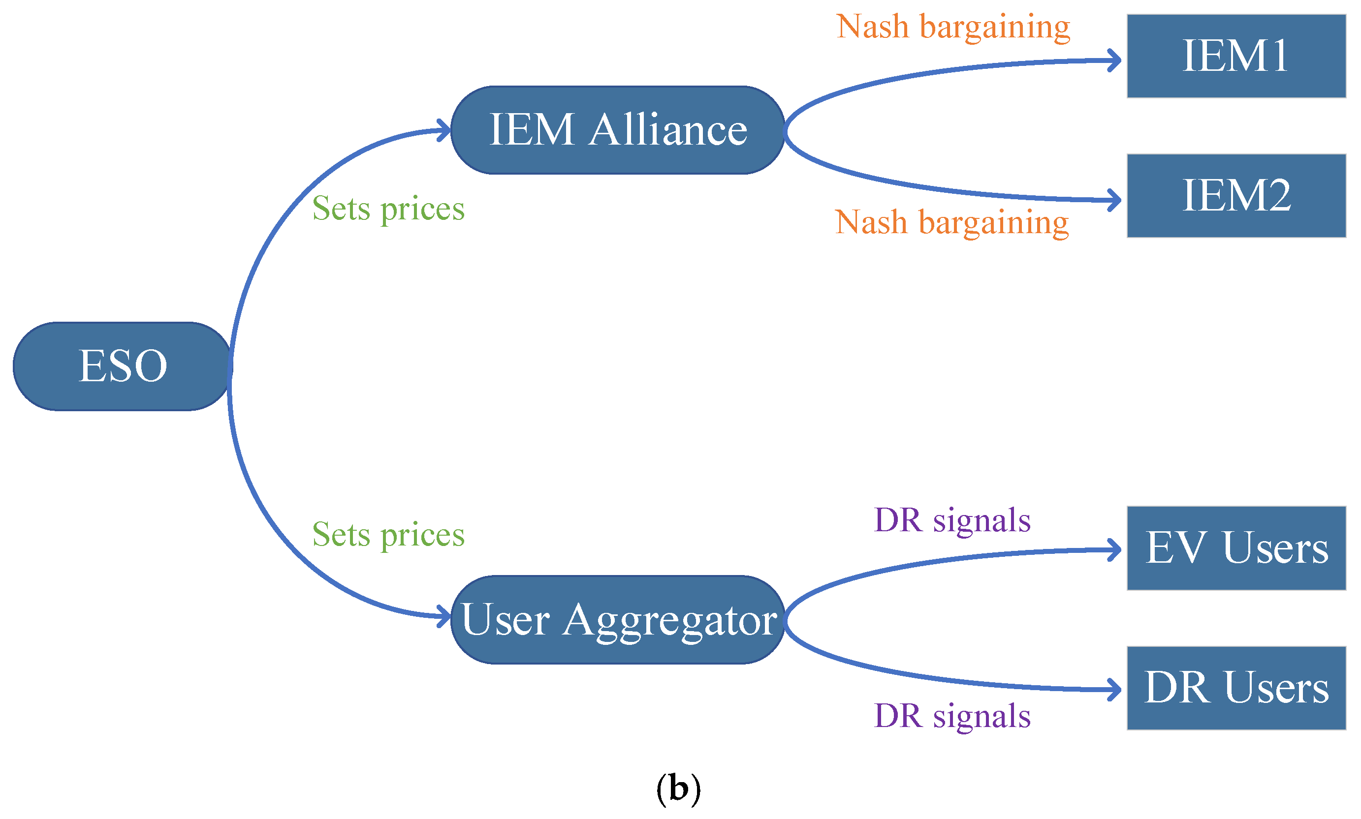
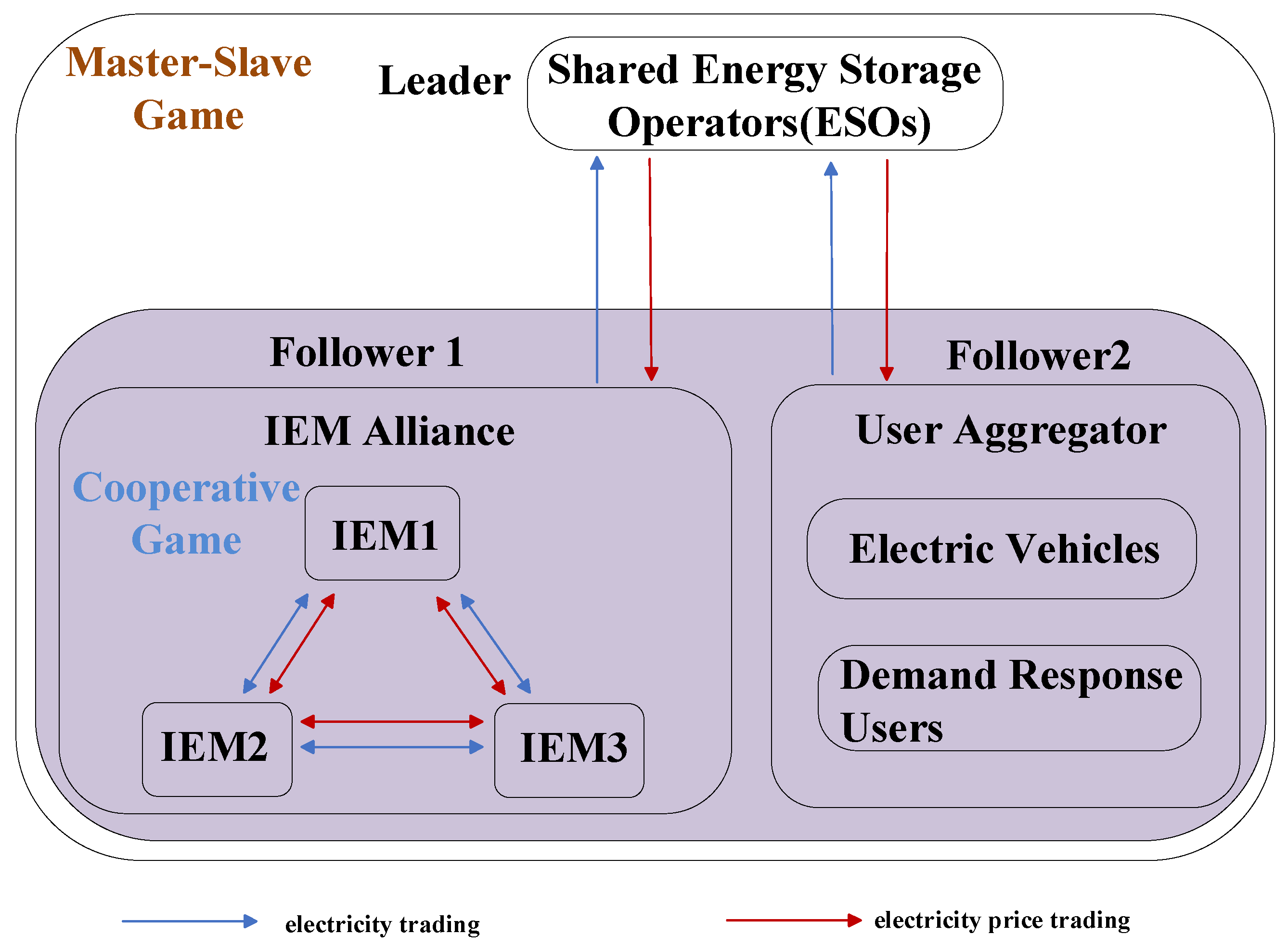
2.1. System Framework

The system model proposed in this paper primarily consists of the higher-level power grid, a shared energy storage operator (ESO), integrated energy microgrid (IEM) aggregators, and multiple types of user aggregators. The detailed framework is illustrated in Figure 1a. The integrated energy system combines both electrical and thermal energy forms, enabling optimal energy allocation and flexible scheduling. The microgrids within the system are capable of conducting electricity trading with the shared energy storage system. When a sub-microgrid experiences an excess supply of renewable energy, the surplus electricity can be sold to the shared storage. Additionally, energy trading among sub-microgrids not only facilitates the local consumption of renewable energy but also reduces reliance on power from external distribution grids, thereby improving the overall energy utilization efficiency of the system. In this manner, the system can better leverage local energy resources and enhance its overall operational performance.

The integrated energy microgrid (IEM) comprises electrical energy storage systems, gas boilers (GBs), combined heat and power (CHP) units, wind turbines, and photovoltaic (PV) systems. These components collectively enable the IEM to meet its respective electrical and thermal load demands. Such a system enhances operational efficiency and promotes more effective resource utilization.

For user aggregators, this paper considers two specific types of user-side participants: electric vehicle (EV) users and demand response (DR) users. The user-side load primarily consists of both electrical and thermal demands. Since the electricity price offered by the shared energy storage operator is assumed to be lower than that of the external grid, this study considers that users exclusively buy and sell electricity from the shared energy storage operator. Each IEM member and user-side entity adjusts its energy price, traded power, and electricity tariffs based on its operational objectives and resource characteristics, and optimizes the output of its internal energy units to effectively meet power and heat demand. This optimization strategy improves the operational efficiency of the system and facilitates the rational allocation of energy resources.

Figure 1b shows the decision hierarchy diagram. The shared energy storage operator (ESO) is the dominant player in the game, setting electricity prices; the microgrid alliance (IEM) and user aggregator (UA) are followers, optimizing their own operations based on electricity prices. At the upper level, the ESO aims to maximize profits by engaging in energy trading with the IEMs and UA under constraints of electricity prices and quantities. At the lower level, each IEM optimizes its electric heating scheduling and energy storage charging and discharging strategies internally, while achieving the fair distribution of electricity transactions within the alliance through the Nash negotiation mechanism. The user aggregator optimizes the charging and discharging behavior and demand response of electric vehicles, balancing comfort and economy. Finally, we equivalently transform the two-layer model into a single-layer optimization problem using KKT conditions; the cooperation problem between IEMs is solved through the ADMM algorithm in a distributed manner.

2.2. Two-Tier Hybrid Game Optimization Framework

The two-layer game framework model is illustrated in Figure 2. The specific steps of the hybrid game process are as follows:

(1)

The ESO engages in a master–slave game with the IEM Alliance and the user aggregator, where all three parties aim to maximize their respective benefits. Through this interaction, the electricity trading prices and power volumes among them are determined, along with the internal power trading volumes among IEM Alliance members.

(2)

Using Nash bargaining theory, the cooperative game problem within the IEM Alliance is decomposed into two subproblems: the aggregator benefit maximization problem and the cooperative benefit allocation problem. Based on the electricity trading volume obtained in step 1, the internal electricity trading price between IEMs is derived according to Nash bargaining principles.

3. Shared Energy Storage Multi-Microgrid Hybrid Game Model with Multiple Types of User Aggregators

3.1. ESO Model for Game Leaders

(1)

Objective function

ESOs aim to maximize their own benefits, which include the costs and benefits of purchasing and selling power with external grids, user aggregators, and the IEM Alliance:

$$\max U^{ESO}=I^{IEM}+I^{UA}-C^{ESO}-C^{TR}$$

(1)

where $U^{ESO}$ is the maximum benefits of the ESO; $I^{IEM}$ is the power interaction gain between the ESO and the IEM Alliance; $I^{UA}$ is the power interaction benefit between the ESO and the user aggregators; $C^{ESO}$ is the charging and discharging cost of the power storage device in the shared energy storage; and $C^{TR}$ is the interaction cost of the shared energy storage with the external power grid:

$$I^{IEM}={\displaystyle \sum _{t=1}^T{\displaystyle \sum _{i=1}^N(p_{IEMi,B}^t}}{P}_{IEMi,B}^t-p_{IEMi,S}^t{P}_{IEMi,S}^t)$$

(2)

$$I^{UA}={\displaystyle \sum _{t=1}^T(p_{UA,B}^t}{P}_{UA,B}^t-p_{UA,S}^t{P}_{UA,S}^t)$$

(3)

$$C^{ESO}=\lambda {\displaystyle \sum _{t=1}^T(P_t^{l,c}}+P_t^{l,d})$$

(4)

$$C^{TR}={\displaystyle \sum _{t=1}^T{p}_t^{D,BUY}{P}_t^{DB}-p_t^{D,SELL}{P}_t^{DS}}$$

(5)

where $p_{IEMi,B}^t$ and $p_{IEMi,S}^t$ are the purchase and sale prices of electricity by of microgrid $i$ to/from the ESO at time t; $P_{IEMi,B}^t$ and $P_{IEMi,S}^t$ are the electricity purchased and sold by the microgrid $i$ to/from the ESO at time t; $p_{UA,B}^t$ and $p_{UA,S}^t$ are the purchase and sale prices of electricity of the user aggregator to/from the ESO at time t; $P_{UA,B}^t$ and $P_{UA,S}^t$ are the electricity purchased and sold by the user aggregator to/from the ESO at time t; $\lambda$ is the charging and discharging cost coefficient of the storage equipment; $P_t^{l,c}$ and $P_t^{l,d}$ are the charging and discharging quantities of the storage equipment of the ESO at time t; $P_t^{DS}$ and $P_t^{DB}$ are the electricity purchased and sold by the ESO from/to the external grid at time t; and $p_t^{D,BUY}$ and $p_t^{D,SELL}$ are the purchasing and selling prices of the ESO from/to the external grid at time t.

(2)

Constraints

The power purchase and sale prices set by the ESO, the amount of power purchased and sold by the ESO from/to the external grid, and the amount of charging and discharging of the energy storage equipment in the ESO should all be within a certain limit range:

$$p_{IEMi,B}^{\min }\le p_{IEMi,B}^t\le p_{IEMi,B}^{\max }$$

(6)

$$p_{IEMi,S}^{\min }\le p_{IEMi,S}^t\le p_{IEMi,S}^{\max }$$

(7)

$$p_{UA,B}^{\min }\le p_{UA,B}^t\le p_{UA,B}^{\max }$$

(8)

$$p_{UA,S}^{\min }\le p_{UA,S}^t\le p_{UA,S}^{\max }$$

(9)

$$P_{\min }^{DS}\le P_t^{DS}\le P_{\max }^{DS}$$

(10)

$$P_{\min }^{DB}\le P_t^{DB}\le P_{\max }^{DB}$$

(11)

$$P_{\min }^{l,c}\le P_t^{l,c}\le P_{\max }^{l,c}$$

(12)

$$P_{\min }^{l,d}\le P_t^{l,d}\le P_{\max }^{l,d}$$

(13)

where $p_{IEMi,B}^{\max }$ and $p_{IEMi,B}^{\min }$ are the upper and lower limits of the purchase price of the IEM Alliance; $p_{IEMi,S}^{\max }$ and $p_{IEMi,S}^{\min }$ are the upper and lower limits of the sale price of the IEM Alliance; $p_{UA,B}^{\max }$ and $p_{UA,B}^{\min }$ are the upper and lower limits of the purchase price of the UA; $p_{UA,S}^{\max }$ and $p_{UA,S}^{\min }$ are the upper and lower limits of the sale price of the UA; $P_{\max }^{DS}$ and $P_{\min }^{DS}$ are the upper and lower limits of the amount of electricity sold by the ESO to the external grid; $P_{\max }^{DB}$ and $P_{\min }^{DB}$ are the upper and lower limits of the amount of electricity purchased by the ESO from the external grid; $P_{\max }^{l,c}$ and $P_{\min }^{l,c}$ are the upper and lower limits of the charging amount of the energy storage device in the ESO; and $P_{\max }^{l,d}$ and $P_{\min }^{l,d}$ are the upper and lower limits of the discharging amount of the energy storage device in the ESO.

In addition, in order to avoid ESOs always choosing the highest energy sale price for their own benefit, it is necessary to constrain the average value of the purchase and sale price of electricity for the IEM Alliance as well as for the user aggregator:

$${\displaystyle \sum _{t=1}^T{p}_{IEMi,B}^t}/24\le p_{IEMi,B}^{ave}$$

(14)

$${\displaystyle \sum _{t=1}^T{p}_{IEMi,S}^t}/24\le p_{IEMi,S}^{ave}$$

(15)

$${\displaystyle \sum _{t=1}^T{p}_{UA,B}^t}/24\le p_{UA,B}^{ave}$$

(16)

$${\displaystyle \sum _{t=1}^T{p}_{UA,S}^t}/24\le p_{UA,S}^{ave}$$

(17)

where $p_{IEMi,B}^{ave}$ and $p_{IEMi,S}^{ave}$ are the average value constraints on the power purchase and sale prices of the microgrid $i$, respectively. $p_{UA,B}^{ave}$ and $p_{UA,S}^{ave}$ are the constraints on the average values of the power purchase and sale prices for the user aggregator, respectively.

Meanwhile, ESO operation should satisfy the following constraints:

$$SOC(t)=SOC(t-1)+({\eta }^{ESO,\mathrm{cha}}{P}_{ESO}^{\mathrm{cha}}(t)-{\displaystyle \frac{P_{ESO}^{dis}(t)}{{\eta }^{ESO,\mathrm{dis}}}})\Delta t$$

(18)

$$SO{C}^{\min }\le SOC(t)\le SO{C}^{\max }$$

(19)

where $SOC(t)$ indicates the residual available charge state of the ESO (state of charge, SOC); ${\eta }^{ESO,\mathrm{cha}}$ and ${\eta }^{ESO,\mathrm{dis}}$ are the charging and discharging efficiencies of the shared energy storage, respectively; $P_{ESO}^{\mathrm{cha}}(t)$ and $P_{ESO}^{dis}(t)$ are the charging and discharging power of the shared energy storage at time $t$, respectively; $\Delta t$ is the time interval from one moment $t$ to the next moment $t+1$; $SO{C}^{\min }$ and $SO{C}^{\max }$ are the minimum and maximum charging states of the ESO, respectively; $SOC(0)$ is the initial energy storage capacity; and $SOC(T)$ is the final energy storage capacity.

The electric power balance constraints for the shared energy storage are as follows:

$$\begin{array}{c}{P}_t^{l,c}-P_t^{l,d}+P_t^{DB}-P_t^{DS}={\displaystyle \sum _{i=1}^N(P_{IEMi,S}^t-P_{IEMi,B}^t)}\\ +P_{UA,S}^t-P_{UA,B}^t\end{array}$$

(20)

3.2. Game Follower IEM Aggregate Modeling

As a follower in the game, the IEM Alliance feeds back the optimized purchased and sold electricity quantities to the ESO based on the tariffs for purchasing and selling electricity set by the ESO. Through this process, the IEM Alliance can adjust its operational strategy based on the tariff signals to maximize its benefits.

(1)

Objective function

IEM Alliance members aim to maximize their own benefits, which include the benefits of purchasing and selling electricity with shared storage, the cost of gas consumption for CHP and GBs, and the cost of charging and discharging storage equipment:

$$\max U^{IEMi}=I_i^{TRADE}+I_{IEMi}^{ESO}-C_i^{GAS}-C_i^{ES}$$

(21)

where $U^{IEMi}$ is the consolidated revenue of $IEMi$; $I_{IEMi}^{ESO}$ is the revenue from the purchase and sale of electricity of $IEMi$; $C_i^{GAS}$ is the cost of gas consumption of CHP and GBs; and $C_i^{ES}$ is the cost of charging and discharging power storage equipment:

$$I_i^{TRADE}={\displaystyle \sum _{t=1}^T{\displaystyle \sum _{j=1,j\ne i}^N(u_{i-j,t}}}{P}_{i-j,t}^{P2P})$$

(22)

$$I_{IEMi}^{ESO}={\displaystyle \sum _{t=1}^T(p_{IEMi,S}^t}{P}_{IEMi,S}^t-p_{IEMi,B}^t{P}_{IEMi,B}^t)$$

(23)

$$C_i^{GAS}={\displaystyle \sum _{t=1}^T\omega (P_{i,t}^{CHP}+P_{i,t}^{GB}})$$

(24)

$$C_i^{ES}={\displaystyle \sum _{t=1}^T\mu (}{P}_{i,t}^{e,c}+P_{i,t}^{e,d})$$

(25)

where $\omega$ is the purchase cost per unit of gas; $P_{i,t}^{CHP}$ and $P_{i,t}^{GB}$ are the amount of natural gas consumed by the CHP and GBs of $IEMi$; $\mu$ is the operation and maintenance cost of the storage equipment; $P_{i,t}^{e,c}$ and $P_{i,t}^{e,d}$ are the charging and discharging amounts of the storage equipment of $IEMi$; $I_i^{TRADE}$ is the sum of the benefits of the interactions between $IEMi$ and the other $IEM$; $u_{i-j,t}$ is the price of the electricity traded between $IEMi$ and $IEMj$ at the time of $t$; and $P_{i-j,t}^{P2P}$ is the amount of electricity traded between $IEMi$ and $IEMj$ at the time of $t$.

(2)

Constraints

(1) The interactive power constraints between microgrids and service providers are as follows:

$$0\le P_{IEMi,B}^t\le P_{IEMi,B}^{\max }$$

(26)

$$0\le P_{IEMi,S}^t\le P_{IEMi,S}^{\max }$$

(27)

$$P_{M2A}^t=P_{IEMi,B}^t-P_{IEMi,S}^t$$

(28)

where $P_{IEMi,B}^{\max }$ and $P_{IEMi,S}^{\max }$ are the maximum purchased and sold power of $IEMi$, respectively, and $P_{M2A}^t$ is the equivalent interaction power from the microgrid to the shared energy storage.

(2) The operational constraints of CHP/GBs are as follows:

$$P_{e,i,t}^{CHP}={\delta }^1\gamma P_{i,t}^{CHP}$$

(29)

$$P_{e,i,t}^{CHP,\min }\le P_{e,i,t}^{CHP}\le P_{e,i,t}^{CHP,\max }$$

(30)

$$P_{h,i,t}^{CHP}={\delta }^2\gamma P_{i,t}^{CHP}$$

(31)

$$P_{h,i,t}^{GB}={\delta }^3\gamma P_{i,t}^{GB}$$

(32)

$$P_{h,i,t}^{GB,\min }\le P_{h,i,t}^{GB}\le P_{h,i,t}^{GB,\max }$$

(33)

where $P_{e,i,t}^{CHP}$ is the power generation of CHP in $IEMi$; ${\delta }^1$ is the conversion efficiency of CHP; $\gamma$ is the heat generated per unit volume of fuel combustion; $P_{e,i,t}^{CHP,\max }$ and $P_{e,i,t}^{CHP,\min }$ are the upper and lower limits of the power generation of CHP in $IEMi$; $P_{h,i,t}^{CHP}$ is the heating power of CHP in $IEMi$; ${\delta }^2$ is the conversion efficiency of CHP; $P_{h,i,t}^{GB}$ is the heating power of the GBs in $IEMi$; ${\delta }^3$ is the conversion efficiency of the GBs; and $P_{h,i,t}^{GB,\max }$ and $P_{h,i,t}^{GB,\min }$ are the upper and lower limits of the heating power of the GBs in $IEMi$.

(3) The operational constraints on the power storage equipment are as follows:

$$E_i^{ES}(t)=E_i^{ES}(t-1)+P_{i,t}^{e,c}{\eta }_i^{ES,cha}-{\displaystyle \frac{P_{i,t}^{e,d}}{{\eta }_i^{ES,dis}}}$$

(34)

$$E_{ES,i}^{\min }\le E_i^{ES}(t)\le E_{ES,i}^{\max }$$

(35)

$$E_i^{ES}(0)=E_i^{ES}(T)$$

(36)

$$0\le P_{i,t}^{e,c}\le P_{i,\max }^{e,c}$$

(37)

$$0\le P_{i,t}^{e,d}\le P_{i,\max }^{e,d}$$

(38)

where $E_i^{ES}(t)$ is the storage capacity of $IEMi$ at moment $t$; ${\eta }_i^{ES,cha}$ and ${\eta }_i^{ES,dis}$ are the charging and discharging efficiency; $E_{ES,i}^{\max }$ and $E_{ES,i}^{\min }$ are the upper and lower limits of the storage capacity; and $P_{i,\max }^{e,c}$ and $P_{i,\max }^{e,d}$ are the maximum charging and discharging constraints.

(4) Inter-IEM P2P electrical energy trading constraints:

P2P electrical energy transactions need to ensure that their volumes are within the limits and equal between IEMs:

$$\left\{\begin{array}{l}-P_{\max }^{P2P}\le P_{i-j,t}^{P2P}\le P_{\max }^{P2P}\\ P_{i-j,t}^{\mathrm{P}2\mathrm{P}}+P_{j-i,t}^{\mathrm{P}2\mathrm{P}}=0\end{array}\right.$$

(39)

where $P_{\max }^{P2P}$ is the maximum interaction limit between IEMs.

(5) Electro-thermal power balance constraints considering renewable energy uncertainties:

In practical applications, the uncertainty of renewable energy sources often has an impact on systems. Therefore, for this problem, corresponding measures need to be taken to cope with and optimize the problem, using Wasserstein-distance-driven fuzzy sets in order to construct distributionally robust chance constraints (specific references [22,23]).

(a) Fuzzy sets based on Wasserstein distance:

First construct the Wasserstein distance $\mathrm{W}(p,\stackrel{\sim }{P})$ between the empirical distribution $\tilde{P}$ and any other probability distribution $p$, defined as follows:

$$W(p,\tilde{P})=\underset{Q}{\inf }\left\{{{\displaystyle \int }}_{{\Xi }^2}\xi -\tilde{\xi }Q(\mathrm{d}\xi ,\mathrm{d}\tilde{\xi })\right\}$$

(40)

where $\Xi$ is the support set of uncertain variable $\xi$, and $Q$ is the joint distribution of $\xi$ and $\tilde{\xi }$. In this paper, the new energy output fuzzy set $D$ can be expressed as

$$D=\left\{\begin{array}{c}p\in \psi (\Xi ):W(p,\tilde{P})⩽\epsilon \end{array}\right\}$$

(41)

to ensure an exact distribution within the fuzzy set with a radius of

$$\epsilon (N)=D\sqrt{{\displaystyle \frac{1}{N}}\ln \left({\displaystyle \frac{1}{1-\beta }}\right)}$$

(42)

where D is a constant that can be obtained by solving the following optimization problem:

$$D=\underset{\rho \ge 0}{\min }\sqrt{{\displaystyle \frac{2}{\rho }}\left(1+\ln \left({\displaystyle \frac{1}{N}}\sum _{m=1}^N{e}^{\rho \parallel {\widehat{\xi }}_m-\widehat{\mu }{\parallel }_1^2}\right)\right)}$$

(43)

where ${\stackrel{\wedge }{\xi }}_m$ represents N historical samples and $\stackrel{\wedge }{\mu }$ is the sample mean of $\stackrel{\wedge }{\xi }$.

(b) DRCC model conversion:

In this paper, we combine the Distributionally Robust Optimization (DRO) method and opportunity constraints to construct a DRCC model and formulate the following opportunity constraints:

$${\inf }_{p\in D}P(0⩽P_t^{\mathrm{WT}}+P_t^{PV}⩽P_t^{REW})⩾1-\alpha$$

(44)

where $\alpha$ is the violation probability, while the sum of the power generated by the turbine and PV systems must be less than the total generation output. After a series of transformations, we obtain the following distributionally robust chance-constrained problem:

$$\left\{\begin{array}{l}\underset{{\underset{¯}{P}}_t^{REW}}{\max }{\displaystyle \sum {\underset{¯}{P}}_t^{REW}}\\ \mathrm{s}.\mathrm{t}.\left\{\begin{array}{l}\alpha N^{REW}{\nu }_t-{\displaystyle \sum _{m=1}^{N^{REW}}{{\rm Z}}_{t,m}\ge \epsilon N^{REW}}\\ -{\underset{¯}{P}}_t^{REW}+{\stackrel{⏜}{P}}_{t,m}^{REW}+M{q}_{t,m}\ge {\nu }_t-{{\rm Z}}_{t,m}\\ M(1-q_{t,m})\ge {\nu }_t-{{\rm Z}}_{t,m}\\ q_{t,m}\in \left\{0,\left.1\right\},{{\rm Z}}_{t,m}\ge 0\right.\end{array}\right.\end{array}\right.$$

(45)

where ${\underset{¯}{P}}_t^{REW}$ is the robust lower bound of renewable energy output power.

The solution to the robust lower bound of the output power of renewable energy sources can be found through the above equation, from which it can be substituted into the electro-thermal power balance constraint as follows:

$$\begin{array}{c}{\displaystyle \sum _{j=1,j\ne i}^N{P}_{i-j,t}^{P2P}-P_{e,i,t}^{CHP}}+P_{i,t}^{l,p}-(P_{IEMi,B}^t-P_{IEMi,S}^t)\\ -(P_{i,t}^{e,d}-P_{i,t}^{e,c})\le {\underset{¯}{P}}_t^{REW}\end{array}$$

(46)

$$P_{h,i,t}^{CHP}+P_{h,i,t}^{GB}=P_{i,t}^{l,h}$$

(47)

where $P_{i,t}^{l,p}$ is the electrical load in $IEMi$ and $P_{i,t}^{l,h}$ is the thermal load in $IEMi$.

(6) Intuitive explanation of Wasserstein-based DRCC superiority:

Compared with traditional chance constraint methods and Conditional Value-at-Risk (CVaR) approaches, Wasserstein-distance-based distributionally robust chance constraints (DRCCs) provide enhanced robustness and generalization ability. Conventional chance constraints assume that the probability distribution of renewable energy uncertainty is known exactly, which is often unrealistic in practical scenarios due to limited or noisy data. CVaR, while useful for tail-risk control, still relies heavily on accurate distributional assumptions and can be sensitive to outliers.

In contrast, Wasserstein-based DRCC models construct an ambiguity set around the empirical distribution obtained from historical data, which contains all plausible distributions within a Wasserstein ball. This approach captures distributional uncertainty directly and ensures that the constraint holds under the worst-case distribution within this set. As a result, the system becomes more robust against data uncertainty, especially under small sample sizes or changing distributions. This is particularly important in microgrid operations where renewable energy outputs (e.g., wind and PV) are highly volatile and difficult to model precisely. Therefore, the Wasserstein-based DRCC method adopted in this paper leads to more reliable decision-making under conditions of uncertainty.

3.3. Game Follower User Aggregator Modeling

3.3.1. Model of EV Charging Station

A cluster model of multiple types of EVs in an EV system can capture the actual operating status of a charging station more effectively than a single EV model. In this paper, five different initial power levels, arrival times, and departure times are listed to represent different types of EVs.

(1) Constraints

$$\left\{\begin{array}{c}0\le P_{n,t}^{\mathrm{ev},\mathrm{cha}}\le P_n^{\mathrm{ev},\mathrm{cha},\max }{i}_{n,t}\\ 0\le P_{n,t}^{\mathrm{ev},\mathrm{dis}}\le P_n^{\mathrm{ev},\mathrm{dis},\max }{i}_{n,t}\\ S_{n,t}=S_{n,t-1}+({\eta }^{\mathrm{EV},\mathrm{cha}}{P}_{n,t}^{\mathrm{ev},\mathrm{cha}}-{\displaystyle \frac{P_{n,t}^{\mathrm{ev},\mathrm{dis}}}{{\eta }^{\mathrm{EV},\mathrm{dis}}}})\mathsf{\Delta }t\\ 0.2S_{n,t}^{oc}{i}_{n,t}\le S_{n,t}\le 0.95S_{n,t}^{oc}{i}_{n,t}\\ S_{n,t}^{\exp }=0.95S_{n,t}^{oc}\end{array}\right.$$

(48)

where $P_{n,t}^{\mathrm{ev},\mathrm{cha}}$ and $P_{n,t}^{\mathrm{ev},\mathrm{dis}}$ are the charging and discharging amount of each type of EV;$P_n^{\mathrm{ev},\mathrm{cha},\max }$ and $P_n^{\mathrm{ev},\mathrm{dis},\max }$ are the upper and lower limits of charging and discharging amount for each type of EV; $i_{n,t}$ is the 0–1 variable of the charging and discharging process; $S_{n,t}$ is the residual power amount of each type of EV; ${\eta }^{\mathrm{EV},\mathrm{cha}}$ and ${\eta }^{\mathrm{EV},\mathrm{dis}}$ are the charging and discharging efficiencies of the EVs; and $S_{n,t}^{oc}$ is the size of the battery capacity of each type of EV. $S_{n,t}^{\exp }$ is the remaining power when the EV leaves.

(2) Electric Vehicle Charging and Discharging Satisfaction Calculation

$$SA{T}_n{=\mathrm{UT}}_{n,t}({\eta }^{\mathrm{EV},\mathrm{cha}}{P}_{n,t}^{\mathrm{ev},\mathrm{cha}}-{\displaystyle \frac{P_{n,t}^{\mathrm{ev},\mathrm{dis}}}{{\eta }^{\mathrm{EV},\mathrm{dis}}}})$$

(49)

where $SA{T}_n$ is charge/discharge satisfaction and ${\mathrm{UT}}_{n,t}$ is the unit utility of each type of electric vehicle.

3.3.2. DR User Model

The second user-side type considered in this paper is the DR user, in which the electrical loads are mainly categorized into transferable loads and curtailable loads. Meanwhile, the two types of electric loads should meet the following requirements:

$$\left\{\begin{array}{l}0\le P_t^{cut}\le P^{cut,\max }\\ 0\le P_{up,t}^{tran}\le P_{up}^{tran,\max }\\ 0\le P_{down,t}^{tran}\le P_{down}^{tran,\max }\\ {\displaystyle \sum _{t=1}^T{P}_{up,t}^{tran}={\displaystyle \sum _{t=1}^T{P}_{down,t}^{tran}}}\end{array}\right.$$

(50)

where $P_t^{cut}$ is the curtailable load, $P^{cut,\max }$ is the maximum value of the curtailable load,$P_{up,t}^{tran}$ is the transferable load (transferred in), $P_{down,t}^{tran}$ is the transferable load (transferred out), and $P_{up}^{tran,\max }$ and $P_{down}^{tran,\max }$ are the maximum values of the transferable load transferred in and transferred out, respectively. At the same time, the total amount of the transferred load of the DR users is 0.

The heat load of DR users is mainly in the form of smart buildings, where the temperature at a certain point in time in the building depends on the previous temperature, the current heat load, and the temperature outside the building.

$$TE{M}_{in}(t)={\lambda }_{1}TE{M}_{in}(t-1)+{\lambda }_2{H}_t^l+{\lambda }_{3}TE{M}_{out}(t)$$

(51)

where ${\lambda }_1$, ${\lambda }_2$, and ${\lambda }_3$ are the weighting coefficients of the temperature of the last time period, the current heat load, and the temperature outside the building, respectively. At the same time, the indoor temperature should also meet the following requirements:

$$\left\{\begin{array}{l}-TE{M}_{in}^{\max }\le TE{M}_{in}(t)-TE{M}_{in}^{opt}\le TE{M}_{in}^{\max }\\ {\displaystyle \sum _{t=1}^{T}TE{M}_{in}(t)}/T=TE{M}_{in}^{opt}\\ 0\le H_t^l\le H_t^{l,\max }\\ {\displaystyle \sum _{t=1}^T\left(\left.TE{M}_{in}(t)-TE{M}_{in}^{opt}\right)\right.={\displaystyle \sum _{t=1}^T\left(AU{X}_t^{plus}-AU{X}_t^{\min \mathrm{us}}\right)}}\\ 0\le AU{X}_t^{plus}\\ 0\le AU{X}_t^{\min \mathrm{us}}\end{array}\right.$$

(52)

where $TE{M}_{in}^{\max }$ is the upper limit of the temperature in the building; $H_t^{l,\max }$ is the upper limit of the heat load of the intelligent building; $AU{X}_t^{plus}$ and $AU{X}_t^{\min \mathrm{us}}$ are values above and below the initial temperature, respectively; and $TE{M}_{in}^{opt}$ is the ideal indoor temperature.

3.3.3. User Aggregator General Model

The electric power balance constraints for user aggregators are as follows:

$$\begin{array}{l}N{P}_{n,t}^{\mathrm{ev},\mathrm{cha}}RAT(n)-N{P}_{n,t}^{\mathrm{ev},\mathrm{dis}}RAT(n)+P_t^l-P_t^{cut}+\\ P_{up,t}^{tran}-P_{down,t}^{tran}+H_t^l/\phi -(P_{UA,B}^t-P_{UA,S}^t)\le {\underset{¯}{P}}_t^{REW,UA}\end{array}$$

(53)

$$RAT(n)=N_n^{EV}/N$$

(54)

where $N$ is the total number of electric vehicles; $RAT(n)$ is the ratio of each type of vehicle to the total; $N_n^{EV}$ is the total number of vehicles in each type; $P_t^l$ is the DR customers’ electric load; $\phi$ is the efficiency of electricity-to-cogeneration switching; $P_{UA,B}^t$ and $P_{UA,S}^t$ are the electricity purchased and sold by the customer’s aggregator to the ESO, respectively; and ${\underset{¯}{P}}_t^{REW,UA}$ is the robust lower bound of the customer-side renewable energy output power.

The objective function of the user aggregator is as follows:

$$\max U^{UA}={\displaystyle \sum _{t=1}^T{\displaystyle \sum _{n=1}^5\left(\begin{array}{l}{p}_{UA,S}^t{P}_{UA,S}^t-p_{UA,B}^t{P}_{UA,B}^t-\\ \left({\psi }_1{P}_t^{cut}+{\psi }_2(P_{up,t}^{tran}+P_{down,t}^{tran})\right)\\ -{\psi }_3\left(AU{X}_t^{plus}+AU{X}_t^{\min \mathrm{us}}\right)\\ +NSA{T}_{n}RAT(n)\end{array}\right)}}$$

(55)

where ${\psi }_1$, ${\psi }_2$, and ${\psi }_3$ are the cost factors for curtailable loads, transferable loads, and temperature deviations, respectively, and $AU{X}_t^{plus}$ and $AU{X}_t^{\min \mathrm{us}}$ are values above and below the initial temperature, respectively.

3.4. IEM Alliance Nash Negotiation Model

The goal of the IEM Alliance is to maximize benefits and respond to ESO decisions through the cooperation of its internal members. In this process, the sub-micro-networks within the IEM Alliance need to maintain cooperation while also ensuring that their own interests are not compromised. To effectively promote reasonable interactions among the sub-micro-networks within the IEM Alliance, this paper introduces Nash negotiation theory as the core tool of cooperative game theory within the micro-network aggregator, aiming to achieve mutual benefit and a win–win situation. Based on this theory, this paper constructs a Nash negotiation model for IEM Alliances, as shown in Equation (56), where the product solution of the model corresponds to the Pareto equilibrium solution of cooperation.

$$\left\{\begin{array}{c}\max \left({\displaystyle \prod _{i=1}^N}\left(U_i-U_i^0\right)\right)\\ \mathrm{s}.\mathrm{t}.U_i\ge U_i^0\end{array}\right..$$

(56)

where $U_i$ is the benefit gained by $IEMi$ participating in negotiations and $U_i^0$ is the benefit gained by $IEMi$ not participating in negotiations, i.e., the point at which negotiations break down.

3.4.1. Subproblem 1: Aggregate Benefit Maximization

$$\left\{\begin{array}{l}\max U^{\mathrm{IEM}}={\displaystyle \sum _{i=1}^N}[I_{IEMi}^{ESO}-(C_i^{\mathrm{GAS}}+C_i^{ES})]\\ \mathrm{s}.\mathrm{t}.\mathrm{formulas}(23)–(38),\mathrm{formula}(46)\end{array}\right.$$

(57)

where $U^{\mathrm{IEM}}$ is the benefit of alliance cooperation.

3.4.2. Sub-Issue 2: Distribution of Benefits from Cooperation

$$\left\{\begin{array}{c}\max {\displaystyle \sum _{i=1}^N}\ln \{{\displaystyle \sum _{t=1,j\ne i}^{24}}[{\displaystyle \sum _{j=1,j\ne i}^N}(u_{i-j,t}{p}_{i-j,t}^{\mathrm{P}2\mathrm{P}\ast })]+U_i^{\mathrm{IEM}\ast }-U_i^0\}\\ \mathrm{s}.\mathrm{t}.{\displaystyle \sum _{t=1}^{24}}[{\displaystyle \sum _{j=1,j\ne i}^N}(u_{i-j,t}{p}_{i-j,t}^{\mathrm{P}2\mathrm{P}\ast })]+U_i^{\mathrm{IEM}\ast }\ge U_i^0\\ u_t^{\mathrm{PS}\ast }\le u_{i-j,t}\le u_t^{\mathrm{PB}\ast }\\ U_i^{\mathrm{IEM}\ast }=I_{IEMi}^{\mathrm{DSO}\ast }-(C_i^{\mathrm{GAS}\ast }+C_i^{ES\ast })\end{array}\right.$$

(58)

where the variable with superscript $\ast$ denotes the optimal solution found in subproblem one.

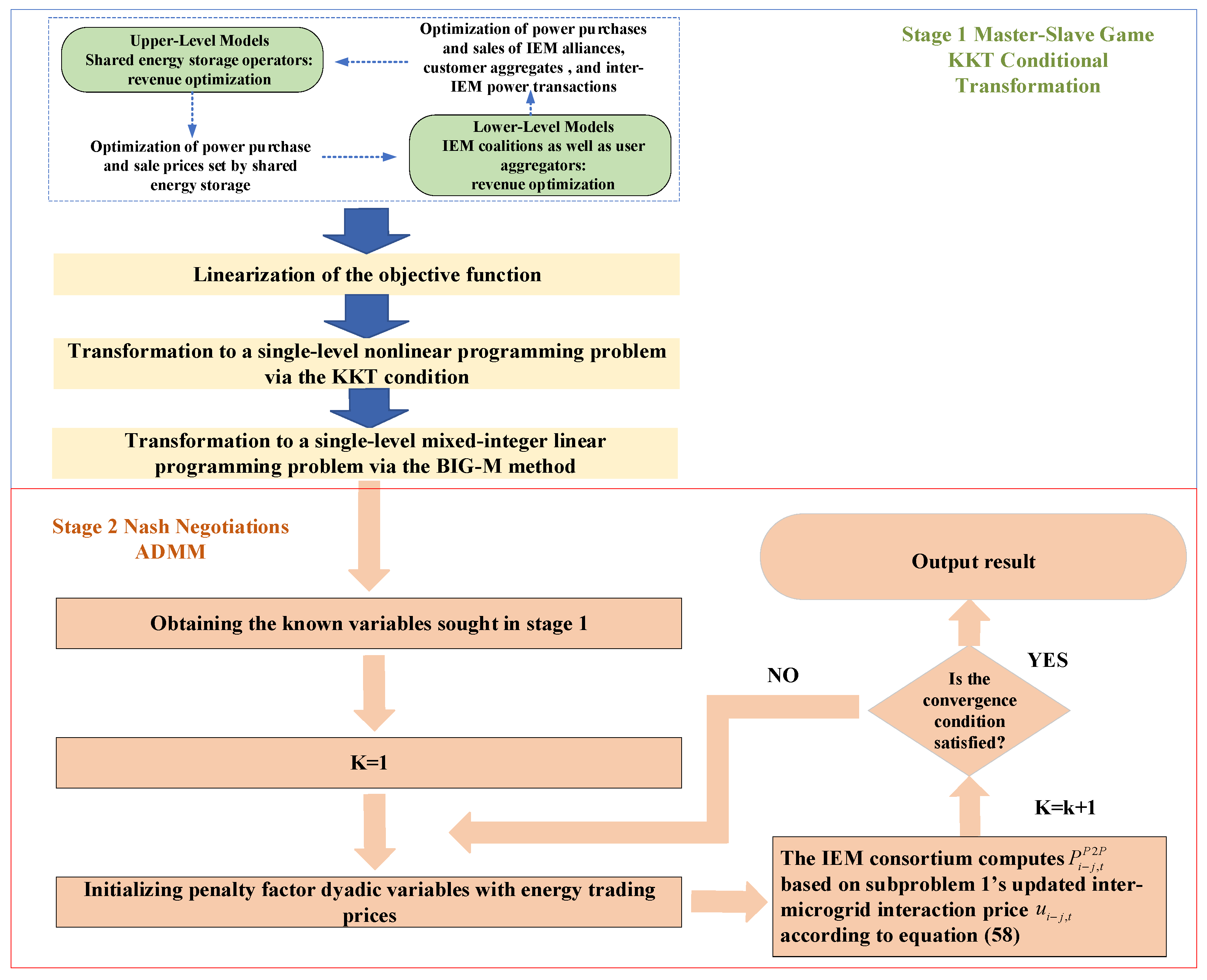
4. Mixed Game Model Solving

In this paper, KKT conditions (specific reference [24]) and the ADMM (specific reference [18]) are used to solve the two phases of the hybrid game separately.

4.1. KKT Condition Solving Master–Slave Game

There are nonlinear terms and nonlinear constraints in the two-layer model constructed in this paper, and there is a coupling relationship between the upper layer and the lower layer of the model, which makes it difficult to be solved directly. Therefore, this paper utilizes KKT conditions as well as the Big-M method to transform the problem into a single-layer mixed-integer linear programming problem, which is easy to solve. The specific formulas are shown in Appendix A. Because the solution process of the user aggregator part is similar to that of the IEM Alliance, only the specific solution formulas of the IEM Alliance are described in Appendix A.

4.2. ADMM Solving IEM Alliance Cooperation Game

The ADMM is used to solve for the optimal electricity interaction price for the IEM Alliance. The interaction price is first decoupled, which leads to

$$u_{i-j,t}=u_{j-i,t}=z_{i-j,t}$$

(59)

where $z_{i-j,t}$ is the shared variable of energy interaction price between $IEMi$ and $IEMj$. The ADMM decomposes the complex optimization problem into several simple subproblems in the following steps:

(1) The $IEMi$ distributed optimization model obtained from the decomposition is

$$\begin{array}{c}\left\{\begin{array}{l}\min L_i=-\ln \left(U_i^0-(u_{i-j,t}{p}_{i-j,t}^{\mathrm{P}2{\mathrm{P}}^{\ast }})+U_i^{\ast }\right)+\\ {\displaystyle \sum _{t=1}^{24}}{\displaystyle \sum _{j=1,j\ne i}^N}\left({\omega }_{i-j,t}(u_{i-j,t}^{\mathrm{P}2\mathrm{P}}-z_{i-j,t})+{\displaystyle \frac{\rho }{2}}{‖u_{i-j,t}^{\mathrm{P}2\mathrm{P}}-z_{i-j,t}‖}_2^2\right)\\ \mathrm{s}.\mathrm{t}.\left\{\begin{array}{c}{\displaystyle \sum _{t=1}^{24}}(u_{i-j,t}{p}_{i-j,t}^{\mathrm{P}2{\mathrm{P}}^{\ast }})+U_i^{\ast }\ge U_i^0\\ U_t^{{\mathrm{PS}}^{\ast }}\le u_{i-j,t}\le U_t^{{\mathrm{PB}}^{\ast }}\end{array}\right.\end{array}\right.\end{array}$$

(60)

where ${\omega }_{i-j,t}$ denotes the dyadic variable between $IEMi$ and $IEMj$, and $\rho$ denotes the penalization factor of the problem.

(2) Each IEM transaction price optimization variable is updated according to the following equation.

$$u_{i-j,t}(k+1)=\arg \min L_i({\lambda }_{i-j,t}(k),u_{i-j,t}(k),u_{j-i,t}(k))$$

(61)

$$u_{j-i,t}(k+1)=\arg \min L_j({\lambda }_{j-i,t}(k),u_{j-i,t}(k),u_{i-j,t}(k+1))$$

(62)

where $u_{i-j,t}(k+1)$ and $u_{j-i,t}(k+1)$ are the K+1th iteration interaction tariffs for microgrids $i$ and $j$, respectively.

(3) ${\lambda }_{i-j,t}$ updates the formula as follows:

$${\lambda }_{i-j,t}(k+1)={\lambda }_{i-j,t}(k)+\rho (u_{i-j,t}(k+1)-u_{j-i,t}(k+1))$$

(63)

where ${\lambda }_{i-j,t}$ is the K+1th multiplier variable.

(4) The convergence condition is determined:

$${{\displaystyle \sum }}_{t=1}^T\parallel u_{i-j,t}(k+1)-u_{j-i,t}(k+1){\parallel }_2^2⩽\epsilon$$

(64)

where $\epsilon$ is the ADMM solution convergence factor.

4.3. Solving Process

The hybrid game-solving process is shown in Figure 3. Stage I is solved by calling the Gurobi solver in MATLAB R2021b using KKT conditions and inputting the solved power purchase, sale price, and inter-IEM electricity trading power into Stage II. Stage II solves the IEMs’ inter-IEM electricity trading price by the ADMM.

5. Calculation Analysis

In this section, the reasonableness of the proposed models is verified through numerical simulations. The parameters used in each model are listed in Appendix B. The power purchase price and feed-in tariff of the ESO are shown in Figure 4, while the electrical and thermal loads of each IEM are presented in Appendix C. The software used in this paper was Matlab R2021b, which called the commercial solvers Cplex and Gurobi for simulation and validation.

5.1. Distribution Robust Boundaries

The parameter $N^{REW}$ within IEM1 in the above equation was defined as 5 (here, IEM1 is used as an example, and the robust boundaries of the remaining parts of the renewable energy sources will not be repeated), this paper set up different violation probabilities $\alpha$, and after solving the problem, the results of each result were compared and analyzed. The results are shown in Figure 5. From Figure 5, it can be seen that increasing the violation probability $\alpha$ will lead to an increase in the lower bound of the renewable energy output power, and on the contrary, decreasing the violation probability $\alpha$ will lead to a decrease in the lower bound of the new energy output power. From this, we conclude that the larger the violation probability $\alpha$ is, the more aggressive the decision made by the system is.

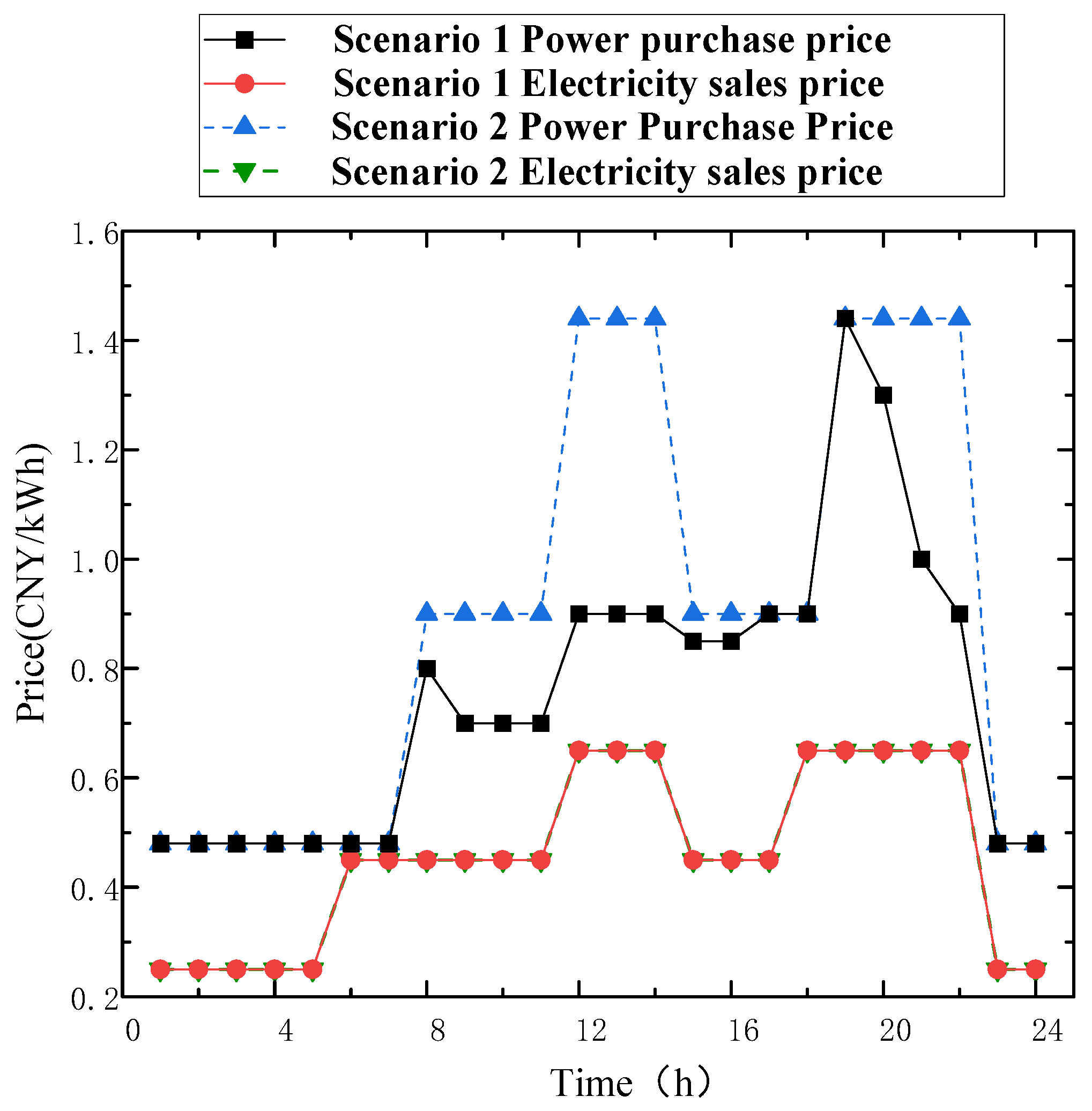
5.2. Comparative Analysis of Different Operational Scenarios

In order to verify the feasibility and effectiveness of the method proposed in this paper, four scenarios were set up for comparison.

Scenario 1: The two-tier game relationship between the ESO and the IEM Alliance with the user aggregator is proposed in this paper, considering the uncertainty of the renewable energy contribution of the IEM Alliance with the user aggregator.

Scenario 2: The master–slave game relationship between the ESO and the IEM Alliance with the user aggregator, disregarding the cooperative game relationship between the IEM Alliance and considering the uncertainty of the renewable energy contribution of the IEM Alliance with the user aggregator.

Scenario 3: A two-tier gaming relationship between the ESO and IEM Alliance and the user aggregator, reducing the scenery outlay by 10% from Scenario 1.

Scenario 4: A two-tier gaming relationship between the ESO and IEM Alliance and the user aggregator, adding a 10% scenery contribution to Scenario 1.

The ESO gains and IEM Alliance and user aggregator costs for each scenario are shown in

Table 1. DSO gains by scenario.

Scheme	ESO Gain/CNY
1	17,264.6022
2	17,503.6768
3	17,494.5814
4	16,954.6514

and

Table 2. IEM Alliance and user aggregator costs by scenario.

Scheme	IEM1 Cost/CNY	IEM2 Cost/CNY	IEM3 Cost/CNY	User Aggregator Cost/CNY
1	36,127.3362	31,635.264	21,454.3989	14,356.6847
2	25,061.197	39,985.1412	24,411.8393	14,356.6847
3	37,033.7154	39,460.2075	16,386.8693	14,421.2247
4	36,262.4284	33,269.1446	18,226.4997	14,319.0811

, respectively.

Comparing Scenario 1 and Scenario 2 in Table 1 and Table 2, Scenario 2 does not consider cooperation between IEM Alliances, which results in members relying excessively on the ESO, thereby increasing power purchases from the ESO. As a result, the ESO’s benefits increase in Scenario 2 compared to Scenario 1, while the operating costs of the IEM Alliance also rise accordingly. This also indicates that peer-to-peer power sharing among IEM Alliance members can effectively reduce the operating costs of the IEM Alliance and improve energy utilization.

Comparing Scenarios 1, 2, 3, and 4 in Table 1 and Table 2, it can be observed that, based on the model proposed in this paper, increasing renewable energy output reduces both integrated operating costs and the ESO’s benefit value. This is because increasing renewable energy output reduces the output power of system components such as combined heat and power (CHP) units and gas boilers, which in turn decreases the amount of power and gas purchased by the IEM Alliance and the user aggregator, thereby leading to a reduction in ESO revenue. It also verifies that increasing renewable energy output contributes to a better low-carbon economy for the system.

The costs and benefits of running the IEM Alliance before and after the collaboration are shown in

Table 3. Costs and benefits before and after IEM cooperation.

IEM Number	Participation in Cooperation Former Cost/CNY	Participation in Cooperation Post-Cost/CNY	Final Score Allocation Cost/CNY	Earnings Upgrade Value/CNY
1	25,061.20	36,127.34	24,908.60	152.60
2	39,985.14	31,635.26	39,832.46	152.68
3	24,411.84	21,454.40	24,259.10	152.74

.

As can be seen from Table 3, the value of benefits for each member of the IEM Alliance before and after cooperation improves by CNY 152.60, CNY 152.68, and CNY 152.74, respectively, which is a total of CNY 458.02. This illustrates that cooperative gaming among IEM Alliances can effectively reduce their respective operating costs.

As can be seen in Figure 6, the final benefit of the ESO increases with an increase in the purchase price of electricity.

5.3. Collaborative Transaction Analysis

5.3.1. Analysis of Shared Energy Storage Operational Results

The power of the shared energy storage interaction with the IEM Alliance and the user aggregator is shown in Figure 7. From Figure 7, it can be seen that the shared energy storage reaches the maximum charging power at 08:00, 09:00, and 10:00, and it reaches the maximum storage capacity at 11:00; it reaches the maximum discharging power at 13:00, 19:00, and 22:00, and is at the minimum storage capacity at 22:00. For the rest of the hours, the shared storage maintains its power balance by trading power with other subjects.

5.3.2. Inter-IEM Transaction Analysis

Shared storage gives the microgrid aggregator a tariff, as shown in Figure 8. The ESO-set tariffs for Scenario 1 and Scenario 2 were analyzed separately. From Figure 8, it can be seen that the ESO-set power purchase tariffs for Scenario 1 are lower than the ESO-set power purchase tariffs for Scenario 2 because Scenario 1 takes into account the IEM Alliance’s energy cooperation transactions more than Scenario 2. As a result, the dependence of each IEM member on the ESO is reduced. At this point, the ESO promotes the IEM to interact with itself by setting lower power purchase tariffs as a way to enhance its own benefits.

The results of the electricity price interaction between the members of each IEM are shown in Figure 9. As can be seen in Figure 9, the interaction tariffs among the IEMs are lower than the power purchase price set by the ESO, and thus the IEMs are able to interact with each other more efficiently in terms of electrical energy.

5.3.3. Analysis of Optimization Results

The optimization results for IEM1 are shown in Figure 10. Observing Figure 10, it can be seen that during the 20:00–4:00 time period, IEM1’s electrical load demand is low and the electricity price set by the ESO is also low; thus, for most of this period, IEM1 opts to purchase electricity from the lower-priced ESO instead of generating its own power. The excess electricity can be stored through energy storage and sold to other microgrids with higher electrical load demand. During the hours of 4:00–8:00, 12:00–13:00, and 17:00–20:00, IEM1’s electrical and thermal load demands increase, and the electricity price set by the ESO rises accordingly. During these times, IEM1 primarily meets its electrical and thermal load demands through combined heat and power (CHP) generation, although exceptions may occur. From 8:00 to 12:00 and 13:00 to 17:00, the demand for electrical and thermal loads reaches its peak, and the electricity price set by the ESO is at its highest. At these times, IEM1’s internal generation is limited, and it must purchase electricity from other IEMs to meet its load requirements. Consequently, the transaction price increases, and IEM1’s energy storage discharges during this period. During the high-load period from 13:00 to 17:00, IEM1 purchases electricity from other grids to satisfy its load requirements. Conversely, during the low-load period from 0:00 to 4:00, IEM1 sells electricity to IEM2 and IEM3 at a high price to generate profit.

The analysis of IEM2 and IEM3 is similar to this stage, so it will not be repeated. The simulation results show that the hybrid game model in this paper effectively realizes the coordinated operation of the subjects within the power grid.

The results of the user aggregator optimization are shown in Figure 11. As shown in Figure 11, during periods of low electricity demand and relatively low electricity prices (such as midnight to 6:00 a.m. and 2:00 p.m. to 6:00 p.m.), user aggregators tend to purchase electricity from the shared energy storage system to meet their own demand or charge electric vehicles; during periods of higher electricity prices (such as the morning peak from 7:00 to 9:00 and the evening peak from 18:00 to 22:00), some electric vehicles are in discharge mode, feeding electricity back to the ESO or other microgrids to generate economic benefits. Additionally, demand response users actively reduce load during high-price periods and delay load activation during low-price periods by adjusting their transferable load and reducible load, effectively lowering electricity costs. Meanwhile, under the premise of ensuring building temperature comfort, by reasonably scheduling thermal load, both economic efficiency and the comfort of thermal energy are achieved.

5.3.4. Analysis of EV Operational Results Within User Aggregator

To further study the characteristics of electric vehicle (EV) clusters, the charging and discharging behaviors of EVs were analyzed, with the specific results shown in Figure 12. The red line in the figure shows the power supply of electric vehicle charging stations.

Combined with the time-of-use tariff, the EV cluster chooses to charge during the low-tariff periods of 0:00–6:00 and 14:00–18:00, and sells electricity to the ESO during the high-tariff periods of 6:00–14:00 and 18:00–22:00 to generate revenue. At the same time, the charging and discharging power boundaries formed by exploiting the dispatchable potential of the EV cluster exhibit strong scalability, providing a foundation for the subsequent upgrading and development of the park.

6. Conclusions

This paper addresses the instability caused by integrating renewable energy generation into distribution grids. It proposes a mixed-game optimization scheduling model that considers the uncertainty of renewable energy generation, involving the ESO, the IEM Alliance, and aggregators of various user types. The two-layer problem is transformed into a single-layer mixed-integer linear programming problem using KKT conditions and the Big-M method to solve the master–slave game, while the lower-layer cooperative game is solved using the ADMM algorithm. The main conclusions are as follows:

First, most existing research models on hybrid games have been based on distribution grids as leaders, with shared energy storage operators as followers or as external factors. This study, however, investigates a one-leader–multiple-followers model in which shared energy storage is the leader and microgrid alliances and user aggregators are both followers. This approach can stimulate the response potential of prosumers, and the analysis results provide guidance for improving the economic efficiency and safety of microgrid operations involving multiple prosumers. Second, this study considers the uncertainty of microgrid alliances and internal renewable energy sources on the user side, and employs distributed robust chance constraints to address this issue. It addresses the problem that as the proportion of renewable energy participating in microgrid operation and scheduling increases, the uncertainty associated with it becomes increasingly evident. And finally, currently, most papers studying user aggregator models tend to treat them as a single type of user, without considering their diversity. To ensure the universality of the user aggregator model, this study considers different types of user models, such as electric vehicle users and demand response users.

Practical Implementation Precautions

Although the proposed hybrid game theory optimization framework demonstrates promising simulation results, its actual deployment requires careful integration into existing microgrid energy management systems. The implementation mainly involves embedding decision logic (such as ESO pricing strategy, IEM bidding mechanism, and user DR) into the hierarchical microgrid energy management system architecture. Firstly, the accurate and real-time measurement of electricity and heat loads, renewable energy output (such as wind speed, solar irradiance), energy storage status (SoC), and market price signals are crucial. We also need historical data to construct a fuzzy set based on Wasserstein distance. Secondly, a bidirectional communication channel must be established between the ESO, IEM, and user aggregator to support decentralized decision-making, electricity price updates, and electricity trading coordination. The integration of the proposed optimization routine into microgrid energy management systems requires sufficient computing resources. This can be solved through cloud-based or edge computing platforms that support real-time KKT and ADMM solvers. Finally, in future work, we can also consider conducting hardware testing or pilot projects on real microgrid test benches to further validate the performance of the framework under real-world communication latency, data uncertainty, and actuator constraints.

References

1. Li, Z.; Meng, F.; Wu, S.; Afthanorhan, A.; Hao, Y. Guiding clean energy transitions in rural households: Insights from China’s pilot low-carbon policies. J. Environ. Manag. 2024, 370, 122782. [Google Scholar] [CrossRef] [PubMed]
2. Bu, X.; Ren, X.; Yin, Y.; Xie, Y. A novel economic dispatch of energy-renewable multi-area power systems with group-based differential evolution. Energy 2024, 313, 134009. [Google Scholar] [CrossRef]
3. Chen, H.; Yang, S.; Wu, H.; Song, J.; Shui, S. Advanced hierarchical energy optimization strategy for integrated electricity-heat-ammonia microgrid clusters in distribution network. Int. J. Hydrogen Energy 2025, 97, 1481–1497. [Google Scholar] [CrossRef]
4. Wan, Y.; Zhang, H.; Hu, Y.; Wang, Y.; Liu, X.; Zhou, Q.; Chen, Z. A novel energy management framework for retired battery-integrated microgrid with peak shaving and frequency regulation. Energy 2024, 313, 133907. [Google Scholar] [CrossRef]
5. Zhang, S.; Hu, W.; Cao, X.; Du, J.; Bai, C.; Liu, W.; Tang, M.; Zhan, W.; Chen, Z. Low-carbon economic dispatch strategy for interconnected multi-energy microgrids considering carbon emission accounting and profit allocation. Sustain. Cities Soc. 2023, 99, 104987. [Google Scholar] [CrossRef]
6. Zhao, B.; Cao, X.; Duan, P. Cooperative operation of multiple low-carbon microgrids: An optimization study addressing gaming fraud and multiple uncertainties. Energy 2024, 297, 131257. [Google Scholar] [CrossRef]
7. Zhang, R.; Bu, S.; Li, G. Multi-market P2P trading of cooling–heating-power-hydrogen integrated energy systems: An equilibrium-heuristic online prediction optimization approach. Appl. Energy 2024, 367, 123352. [Google Scholar] [CrossRef]
8. Li, J.; Liu, D.; Jiang, S.; Wu, L. Optimal configuration of shared energy storage system in microgrid cluster: Economic analysis and planning for hybrid self-built and leased modes. J. Energy Storage 2024, 104, 114624. [Google Scholar] [CrossRef]
9. Lin, S.; Li, T.; Shen, Y.; Li, D.; Zhou, B.; Zhao, J.; Wu, D. Energy sharing optimization strategy of smart building cluster considering mobile energy storage characteristics of electric vehicles. Electr. Power Syst. Res. 2025, 238, 111067. [Google Scholar] [CrossRef]
10. Park, K.-E.; Choi, W.-J.; Kim, H.; Kim, J.; Hong, J.-Y.; Kim, M.-H. Investigation of the energy performance of thermal energy sharing for photovoltaic-thermal systems in a thermal prosumer network. Case Stud. Therm. Eng. 2024, 61, 104881. [Google Scholar] [CrossRef]
11. Yang, H.; Yang, Z.; Gong, M.; Tang, K.; Shen, Y.; Zhang, D. Commercial operation mode of shared energy storage system considering power transaction satisfaction of renewable energy power plants. J. Energy Storage 2025, 105, 114738. [Google Scholar] [CrossRef]
12. Siqin, T.; He, S.; Hu, B.; Fan, X. Shared energy storage-multi-microgrid operation strategy based on multi-stage robust optimization. J. Energy Storage 2024, 97, 112785. [Google Scholar] [CrossRef]
13. Asri, R.; Aki, H.; Kodaira, D. Optimal management of shared energy storage in remote microgrid: A user-satisfaction approach. Renew. Energy Focus 2024, 51, 100635. [Google Scholar] [CrossRef]
14. Xiao, J.-W.; Yang, Y.-B.; Cui, S.; Wang, Y.-W. Cooperative online schedule of interconnected data center microgrids with shared energy storage. Energy 2023, 285, 129522. [Google Scholar] [CrossRef]
15. Qiao, J.; Mi, Y.; Shen, J.; Lu, C.; Cai, P.; Ma, S.; Wang, P. Optimization schedule strategy of active distribution network based on microgrid group and shared energy storage. Appl. Energy 2025, 377, 124681. [Google Scholar] [CrossRef]
16. Li, J.; Yang, Z.; Wu, Z.; Yang, L.; Li, S.; Zhu, Y. Master-slave game-based operation optimization of renewable energy community shared energy storage under the frequency regulation auxiliary service market environment. J. Energy Storage 2024, 103, 114499. [Google Scholar] [CrossRef]
17. Zhang, W.-W.; Wang, W.-Q.; Fan, X.-C.; He, S.; Wang, H.-Y.; Wu, J.-H.; Shi, R.-J. Low-carbon optimal operation strategy of multi-park integrated energy system considering multi-energy sharing trading mechanism and asymmetric Nash bargaining. Energy Rep. 2023, 10, 255–284. [Google Scholar] [CrossRef]
18. Wang, D.; Fan, R.; Xu, X.; Du, K.; Wang, Y.; Dou, X. Hybrid game model for electricity trading and pricing among multiple microgrids and consumers based on demand-side complex networks. Energy 2024, 313, 133961. [Google Scholar] [CrossRef]
19. Li, C.; Liu, Y.; Li, J.; Liu, H.; Zhao, Z.; Zhou, H.; Li, Z.; Zhu, X. Research on the optimal configuration method of shared energy storage basing on cooperative game in wind farms. Energy Rep. 2024, 12, 3700–3710. [Google Scholar] [CrossRef]
20. Gao, J.; Shao, Z.; Chen, F.; Lak, M. Robust optimization for integrated energy systems based on multi-energy trading. Energy 2024, 308, 132302. [Google Scholar] [CrossRef]
21. Lu, S.; Gu, W.; Xu, Y.; Dong, Z.Y.; Sun, L.; Zhang, H.; Ding, S. Unlock the Thermal Flexibility in Integrated Energy Systems: A Robust Nodal Pricing Approach for Thermal Loads. IEEE Trans. Smart Grid 2023, 14, 2734–2746. [Google Scholar] [CrossRef]
22. Li, Y.; Wang, J.; Cao, Y. Multi-objective distributed robust cooperative optimization model of multiple integrated energy systems considering uncertainty of renewable energy and participation of electric vehicles. Sustain. Cities Soc. 2024, 104, 105308. [Google Scholar] [CrossRef]
23. Nguyen, H.T.; Choi, D.H. Distributionally Robust Model Predictive Control for Smart Electric Vehicle Charging Station with V2G/V2V Capability. IEEE Trans. Smart Grid 2023, 14, 4621–4633. [Google Scholar] [CrossRef]
24. Song, L.; Sheng, G. A nonsmooth Levenberg–Marquardt method based on KKT conditions for real-time pricing in smart grid. Int. J. Electr. Power Energy Syst. 2024, 162, 110235. [Google Scholar] [CrossRef]
Figure 1. (a) System model framework diagram. (b) Decision hierarchy chart.
Wevj 16 00401 g001aWevj 16 00401 g001b
Figure 2. Hybrid game two-layer optimization framework diagram.
Wevj 16 00401 g002
Figure 3. Flowchart for solving double-layer game.
Wevj 16 00401 g003
Figure 4. Prices of energy in upper grid.
Wevj 16 00401 g004
Figure 5. Robust boundaries of wind power output distribution.
Wevj 16 00401 g005
Figure 6. Sensitivity analysis of electricity price fluctuations.
Wevj 16 00401 g006
Figure 7. Shared energy storage charging and discharging power and charge state.
Wevj 16 00401 g007
Figure 8. Energy prices of microgrid aggregates developed by master–slave game under different scenarios.
Wevj 16 00401 g008
Figure 9. Interaction tariff curves among IEMs.
Wevj 16 00401 g009
Figure 10. IEM1 optimization results.
Wevj 16 00401 g010
Figure 11. User aggregator optimization results.
Wevj 16 00401 g011
Figure 12. Variation in EV power without each type of EV.
Wevj 16 00401 g012