Battery Charging Simulation of a Passenger Electric Vehicle from a Traction Voltage Inverter with an Integrated Charger

Abstract

This paper presents the results of the mathematical modeling and experimental studies of charging a traction lithium-ion battery of a passenger electric car using an integrated charger based on a traction voltage inverter. An original three-stage charging algorithm (3PT/PN) has been developed and implemented, which provides a sequential decrease in the charging current when the specified voltage and temperature levels of the battery module are reached. As part of this study, a comprehensive mathematical model has been created that takes into account the features of the power circuit, control algorithms, thermal effects and characteristics of the storage battery. The model has been successfully verified based on the experimental data obtained when charging the battery module in real conditions. The maximum error of voltage modeling has been 0.71%; that of current has not exceeded 1%. The experiments show the achievement of a realized capacity of 8.9 Ah and an integral efficiency of 85.5%, while the temperature regime remains within safe limits. The proposed approach provides a high charge rate, stability of the thermal state of the battery and a long service life. The results can be used to optimize the charging infrastructure of electric vehicles and to develop intelligent battery module management systems.

1. Introduction

In the modern world, global challenges to energy security, the need for a sharp reduction in carbon dioxide emissions and the course towards the development of sustainable transport determine one of the most important tasks of our time: a radical improvement in the technology of battery systems of electric vehicles [1,2]. The active increase in the share of electric vehicles in the global car fleet is a natural response to the growing requirements for improving the environmental friendliness of vehicles, the desire for energy efficiency and the strategic reduction of dependence on depleting fossil fuels [3,4]. The transition to electric vehicles is seen as a key element in the fight against climate change and the creation of a more sustainable and secure energy system [5].

Despite significant advances in the development and commercialization of electric vehicles, one of the main constraints to their wider adoption remains the need to ensure the fast, safe and, most importantly, long-lasting charging of traction batteries [6,7]. This challenge requires a comprehensive and innovative approach that covers several key areas. Firstly, it is necessary to develop fundamentally new and improved charging methods that can significantly reduce the time spent on replenishing the battery, without compromising its resource and safety. Secondly, it is necessary to create intelligent energy management systems that will optimize the charging process, taking into account the current operating conditions, battery condition and energy efficiency requirements. Thirdly, an integral part of the solution is the development of the mathematical modeling of the charge and discharge processes, which makes it possible to accurately predict the behavior of the battery in various operating modes, to identify potential problems and to develop optimal control strategies [8,9]. Only an integrated approach that combines these areas will allow overcoming existing limitations and unleashing the full potential of electric vehicles as a key element of a sustainable transport future [10].

1.1. Overview of Electric Vehicle Charger Topologies

To assess the place of the proposed solution in the EV charging infrastructure ecosystem, it is necessary to take a detailed look at the most significant charging topologies used today, analyzing their advantages and limitations.

1.1.1. On-Board Charger (OBC)

On-board chargers are integrated directly into the EV, and they convert the AC grid current to DC to charge the battery. Typical power is 3.3–22 kW and the charging time for a 75 kWh battery ranges between 2.7 and 18 h depending on the charging power of 22–75 kWh [11]. The efficiency of the OBC is ≈90–93% [12], critically dependent on the temperature, battery condition and charge level [13]. The architecture includes a PFC converter and, as a rule, an LLC/DC DC stage for isolation. The OBC provides home and public charging (Level1/2) and is easy to operate, but is limited in power and requires a long charging time. The implementation of bidirectional modes (V2G/V2L) requires additional complex electronics and software.

1.1.2. Off-Board Isolated DC/DC Fast Charger

External (Level3) charging stations are capable of delivering power ranging from 50 to 350 kW owing to high-voltage DC circuits and galvanic isolation. Efficiency reaches 92–95%, provided by filtering, protective circuitry and active cooling [14]. Such stations charge an average battery (~75 kW h) up to 80% in about 20–40 min. Their advantages are high speed, safety, CHAdeMO/CCS standards and support for two-way communication with the network. However, significant disadvantages are large dimensions, the cost of infrastructure and the need for dedicated installation sites.

1.1.3. Non-Isolated Fast Charger (e.g., Interleaved Boost, LLC Resonant)

These devices, with a power of 20–150 kW, implement interleaved boost PFC and LLC or Phase-Shifted Full Bridge topologies, achieving 95–97% efficiency due to soft switching (ZVS) and a high-power density. They are much more compact than isolated stations, but require complex frequency control, phasing and enhanced EMI shielding. The lack of a galvanic isolation makes them less safe without strict measures to suppress leakage currents and protection.

1.1.4. Integrated Charger (iOBC/IBC)

Integrated chargers use the traction inverter and motor windings (usually PMSM) as an active front-end rectifier and filter [15]. The power is in the range of 10–50 kW and efficiency is within 94–96%, achieved by reducing the number of components and overall optimization [16]. The advantages are compactness, reduced weight and cost and readiness for V2G modes. The main difficulties are related to:

• More complex control for switching charging and drive modes.
• Ensuring galvanic isolation (via switches, transformers or a neutral point).
• Avoiding the generation of charging torque (rotation) by means of six- or multi-phase machines or an algorithmic shift of a rotor position [17].
• Increased requirements for EMI and overall system reliability [0search16, 0search3].

In

Table 1. The comparison of EV charger topologies.

Topology	Power Level	Efficiency	Cost	Complexity	Size	Bidirectionality
On-board charger (OBC)	≤22 kW	90–93%	Average	Low	Average	Limited
Off-board isolated DC/DC	50–350 kW	92–95%	High	Average	Big	Supported
Non-isolated fast charger	20–150 kW	95–97%	High	High	Average	Supported
Integrated charger (iOBC/IBC)	10–50 kW	94–96%	Low	High	Low	Supported

, we have compared the topologies of electric vehicle chargers.

One widely used approach to optimizing the charging process is to use the two-stage DC/DC (DC/DC) charging algorithm. This method was used, for example, in [16], where it was implemented to hold the battery at the DC stage until the specified voltage was reached and then to move to the stage of maintaining the voltage until the charge was completed. During these studies, a high fullness of charge was achieved with a moderate time of energy replenishment. However, the use of PT/PN showed a number of drawbacks, including the local overheating of batteries at the DC voltage stage and the accelerated aging of cells, especially at elevated operating temperatures.

Another approach is the use of a pulsed charge in the case of a direct current (PT/IR). Introducing pauses between charge pulses allows the battery to partially recover, lowering the internal temperature and increasing the battery life. A decrease in the degradation of active materials and an increase in the number of permissible charge–discharge cycles by 10–15%, compared to classical PT/PN, have been experimentally recorded. However, this method has the disadvantage of an increased total charge time, which reduces its attractiveness for use in mass transport.

Another promising area is the multi-stage direct current charge (MSPT), which was studied in [16]. This method involves a gradual decrease in the charging current as the degree of charge of the battery increases. Experimental data show a 20% increase in the overall battery life and an increase in the energy efficiency of the charging process [17]. The main disadvantage of the MSPT approach is the complication of the charging management algorithms and the need for the constant monitoring of battery parameters, which increases the requirements for on-board diagnostic systems for electric vehicles [18].

Variations of the PT/PN algorithm with an improved control system were presented in [19]. They introduced additional correction circuits in the current and voltage regulation channel, which made it possible to reduce the charging time by 8–10% without deteriorating the performance of the batteries [20]. However, such modernization requires the use of more complex and expensive electronic components, which increases the cost of chargers [21].

The constant voltage impulse charge (CP/SR) was investigated as a way to combine the benefits of a stable voltage and reduce the heat load on the battery cells [22]. The results showed that with the help of this algorithm, it was possible to reduce the maximum temperature of the batteries during charging by 5–7 °C, which had a positive effect on their durability. At the same time, similar to other pulsed methods, there was an increase in the time of full charge, which limits the scope of this approach [23].

The accelerated charge at an elevated voltage (PNPT/PN) is another area of research. Such methods are aimed at achieving the shortest possible charge time, as shown in [24], but are accompanied by the risks of the overcharging and accelerated aging of batteries, which requires the very precise control of the charge and temperature parameters [25].

Against the background of the above directions, the solution presented in the article under consideration is of particular relevance. The main attention is paid to the application of the original three-stage 3PT/PN charging algorithm, which combines the advantages of a high charging rate and the prolongation of the battery life [26]. A distinctive feature of the proposed approach is a multi-stage reduction in the charging current with the simultaneous monitoring of the battery voltage and temperature, which minimizes the risk of thermal degradation and increases the efficiency of the entire process. The developed three-stage 3PT/PN algorithm provides a high charge rate, stability of the thermal state of the battery and a long service life. The results can be used to optimize the charging infrastructure of electric vehicles and to develop intelligent battery module management systems [27,28]. The use of an integrated charger as part of the traction voltage inverter ensures a rational circuit design and compact integration within the electric vehicle’s power unit, contributing to a reduced weight and overall cost. The proposed three-stage 3PT/PN charging algorithm is based on a rule-driven transition between current stages in response to the real-time battery voltage and temperature measurements. Although the algorithm does not employ model-based predictions or state estimations such as SoC or SoH, it adapts its behavior to actual battery conditions through direct sensing and threshold logic. This provides a balance between practical implementation and control responsiveness. The developed solution enables high charging rates, a stable thermal performance and extended battery service life under constrained computational environments. The presented results can serve as a foundation for the further development of smart battery control systems, including future extensions toward model-predictive or data-driven adaptive control frameworks.

The mathematical model developed as part of the work covers the processes in the charger and in the battery itself, which ensures high accuracy in calculating the parameters of charging. Particular attention is paid to the adaptation of the model to various operating modes, taking into account thermal effects [29], which is especially important for the correct reproduction of the real operating conditions of electric vehicles. The combination of mathematical modeling with experimental studies on a real object allowed the author not only to confirm the adequacy of the developed model, but also to demonstrate its applicability for predicting the characteristics of chargers [30] in a wide range of conditions.

Unlike conventional charging algorithms, such as the classical two-stage constant current/constant voltage (CC/CV or PT/PN) method, which suffers from thermal stress and accelerated aging at the CV stage, the proposed three-stage algorithm introduces a stepwise current reduction strategy that responds dynamically to both voltage and temperature thresholds. Compared to pulse charging methods (PT/IR), which intermittently interrupt the charging current to reduce heat and stress, our algorithm avoids the associated increase in the total charge time while maintaining thermal stability. Additionally, in contrast to advanced multi-stage methods (MSPT) that require complex feedback and diagnostics, our approach achieves similar or superior lifetime extension effects (up to 15–20%) with a significantly simpler control structure. It also outperforms voltage-accelerated fast charge methods (PNPT/PN), which reduce the charge time to ~12 min, but often cause localized overheating and electrode degradation. Our experimental results demonstrate that the proposed algorithm reduces the charge time by up to 17 min while preserving the battery integrity and keeping the temperature well below 30 °C, offering a practical compromise between speed, safety and durability. Therefore, the 3PT/PN method combines the best features of several advanced strategies while minimizing their drawbacks, representing a novel and efficient solution for traction battery charging in passenger EVs.

The authors compiled comparative

Table 2. The key parameters of various algorithms for charging traction lithium-ion batteries, including the author’s proposed 3PT/PN.

Charging Algorithm	Charging Time *	Max. Temperature, °C	Extended Service Life	Energy Efficiency,%	Complexity of Implementation	Comment
PT/PN (CC/CV)	20–25 min	up to 42	Low	83–85	Low	Classic two-stage algorithm, risk of overheating at the CV stage
PT/IR (Pulsating)	30–35 min	≤35	Moderate (+10…–15%)	82–84	Average	Reduced temperature due to pauses, but long overall charging time
MSPT (Multi-Stage DC)	22–28 min	34–36	High (+15…–20%)	84–86	High	Requires complex diagnostics and feedback on all elements
PNPT/PN (Over-Voltage Accelerated)	12–14 min	up to 45	Low/Degradation	87–88	Average	Greatly reduces time, but causes degradation of the electrodes
Proposed 3PT/PN	17 min	≤29.3	High (+15…–20%)	85.5	Low	Combines speed, efficiency and a soft thermal profile

* Approximate values when charging batteries at 85% to a full capacity of 8.9–10 Ah.

, reflecting the key parameters of various algorithms for charging traction lithium-ion batteries, including the author’s proposed 3PT/PN.

To more clearly emphasize the benefits and unique characteristics of the proposed 3PT/PN charging strategy, Table 2 presents a comparative overview of major charging algorithms commonly used or discussed in the recent literature. The table evaluates key performance indicators such as the charge time, peak battery temperature, impact on the battery lifespan, energy efficiency and system implementation complexity. As the results indicate, the 3PT/PN method provides a well-balanced compromise: it reduces the total charge time compared to traditional and pulsed methods while avoiding the thermal stress and cell degradation observed in accelerated high-voltage approaches. Moreover, it achieves high energy efficiency and lifespan extension effects with a relatively simple control structure, making it practical for integration into electric vehicle power systems.

While many industrial battery management systems (BMS) employ variants of current tapering or CC/CV strategies, these implementations often rely on fixed thresholds and do not simultaneously integrate thermal constraints in a predictive manner. The novelty of the proposed 3PT/PN algorithm lies in its explicit integration of both voltage and temperature thresholds as dynamic criteria for current reduction, along with a fixed three-level current staging that is optimized for compact traction modules with a limited cooling capability. Additionally, the algorithm is embedded into a power-inverter-based integrated charger topology, rather than using a separate charging unit, which simplifies the overall hardware and reduces energy conversion losses. This approach is verified through both a detailed simulation and high-resolution experimental validation under quasi-real operating conditions, offering a practical alternative that balances the energy throughput, safety and battery longevity. To the best of our knowledge, this combination of implementation simplicity, thermal adaptability and hardware integration has not been reported in prior works.

The purpose of this work is to mathematically develop a model and to experimentally verify an effective charging algorithm for a traction lithium-ion battery of a passenger electric car based on a three-stage DC/DC voltage algorithm. This will ensure a high charging rate while increasing the service life of batteries and create an integrated charger as part of a traction voltage inverter to improve the overall energy efficiency of the transport system.

2. Methods and Materials

Within the framework of this study, a set of experimental works was carried out, aimed at verifying the developed mathematical model of the charging process of a traction lithium-ion battery of a passenger electric car and the experimental testing of the original three-stage charge algorithm. The general plan of the experimental works provided for the creation of a mathematical model of a charger integrated into the power circuit of a traction voltage inverter [31]. It also considered the development of charge control algorithms, the manufacture of an experimental sample of a traction inverter system with an integrated charger and a series of charging tests on a real battery module [32] of an electric car.

As the basic element of the charging system, a traction voltage inverter with an integrated charger (TPCS) was used, made on the basis of transistor–diode IGBT modules. The basis of the power part of the experimental plant was a semi-bridge inverter assembled on the basis of the Infineon FS75R12KT4 IGBT module [33], designed for an operating voltage of 1200 V and a maximum current of 75 A. This module provides a high switching speed and low switching losses, which is critical for the effective operation of the charger as part of an electric vehicle [34]. The inverter circuit also included elements of damper chains implemented on the basis of RC circuits that protect semiconductor devices from overvoltage during the switching process.

The switching was controlled using CONCEPT 2SC0108T2A0-17 IGBT module control drivers (CT CONCEPT, Bienne, Switzerland), which are characterized by high noise immunity and slow response delay time. These drivers made it possible to generate control signals in accordance with the pulse width modulation algorithms implemented in the control microcontroller [35].

A specialized board based on the Texas Instruments TMS320F28069 microcontroller (Texas Instruments, Dallas, TX, USA), belonging to the C2000 family of digital signal processors, was used as a control. This processor provided the high-speed processing of the battery current and voltage feedback signals and the implementation of PI control algorithms and switching functions according to the developed charge algorithms. The software of the control module was developed in C using the Code Composer Studio development environment [36].

The traction battery of the electric car, on which experimental studies were carried out, was a modular system consisting of several lithium-ion battery modules. Each module was assembled on the basis of NMC (lithium–nickel–manganese–cobalt oxide) battery cells, which had a high specific capacity and durability [37]. The rated voltage of a single module was 45 V and the voltage of a fully charged module reached 50.4 V. The traction battery provided a high energy density and was adapted to operate in a wide range of temperatures.

During the experiments, the main attention was paid to the implementation of a three-stage charge algorithm, which involves three consecutive stages of charging with a direct current followed by reaching the stage of a constant voltage. At the first stage, charging was performed with a current of 50 A until the specified voltage of the battery module was reached. Upon reaching the threshold voltage, the transition was made to the second stage, where the charge current was reduced to 35 A, and then, with a further increase in voltage, to the third stage with a current of 25 A. The main criterion for the transition between the stages was the achievement of the threshold voltage values on the battery modules equal to 50.4 V.

To measure the parameters of the electric current and voltage, Yokogawa high-precision measuring modules of the WT3000E series [38] were used, which provided a current measurement with an accuracy of 0.02% of the measured value and the voltage with an accuracy of 0.01%. These devices made it possible to record changes in the current and voltage at the output of the charger in real time, as well as to calculate the integral characteristics of the charging process, such as the realized capacity and the efficiency of the system [39].

In the experiment, the temperature of the battery modules was monitored using precision digital thermal sensors of the DS18B20 series, connected to the controller via the 1-Wire interface [40]. Temperature data were used to control permissible charge modes and to analyze thermal effects [41] arising during the passage of currents through battery cells.

A schematic diagram of the experimental setup is presented in Figure 1. The experimental system includes a traction voltage inverter with an integrated charger (TPCS), a modular lithium-ion battery based on NMC cells, a control unit built on the TMS320F28069 processor (Texas Instruments, Dallas, TX, USA) and precision sensors (WT3000E and DS18B20) (Maxim Integrated, San Jose, CA, USA) and a cooling and ventilation system. The measurement subsystem and control interface are connected via high-speed isolated channels. Figure 1 provides a visual overview of the spatial arrangement of key components used in the experimental verification of the proposed 3PT/PN charging algorithm.

The experimental setup has the following elements:

-

A traction voltage inverter (TPCS);

-

An integrated charger section;

-

A battery module (NMC, 45–50.4 V);

-

Current and voltage measuring equipment (Yokogawa WT3000E);

-

Temperature sensors (DS18B20);

-

A control board (TMS320F28069);

-

A PC for data logging (optional);

-

A cooling/ventilation unit;

-

Labels on power and signal lines.

Before the start of the experiments, the battery modules were partially discharged to an initial voltage of 48.6 V, which corresponded to a state of charge of about 85%. The average temperature of the modules before the start of charging was 18.5 °C. Charging was conducted under laboratory conditions at an ambient temperature of 20–22 °C using a standard ventilation system to prevent the overheating of the equipment.

A software and hardware complex that provided a record of the time dependencies of the voltage, current, temperature and charge time controlled the charging. The data were recorded with a sampling interval of 0.1 s, which made it possible to obtain detailed dependencies of all monitored parameters for a subsequent analysis and comparison with the results of mathematical modeling [42].

The mathematical model built in the MATLAB/Simulink environment [43] included separate subsystems for modeling the power part of the charger, control system, battery and feedback channels. The power part of the model considered switching losses in IGBT modules [44], parasitic inductances of connections and characteristics of damper chains. The control system was simulated taking into account the real-time delays of the drivers and the controller, and the battery was described using a modified Shepherd model [45], supplemented by temperature corrections.

In mathematical modeling, special attention was paid to the precise adjustment of the coefficients of PI-regulators of the current and voltage [46] to achieve the high stability of the control processes. The parameters of the battery model, including the initial voltage, capacity, internal resistance and temperature coefficients [47], were determined on the basis of preliminary experimental tests.

During the experiments, various charge modes were used: a standard two-stage PT/PN charge and the original 3PT/PN three-stage algorithm. The results obtained experimentally and calculated according to the mathematical model were compared for each of the modes. The evaluation criteria were the maximum deviations of the voltage and current between the model and experimental data at all stages of charge [48]. To quantify the convergence, a calculation error was used, expressed as a percentage of the experimental value.

As a result of the experimental work, the high compliance of the model with real processes was confirmed [49]. The maximum error in determining the voltage using the 3PT/PN algorithm was 0.71% and it did not exceed 1% for the current. A significant discrepancy between the calculated and experimental data was noted only at the initial moments of charge and during the final reduction of the current to zero, which is explained by the specifics of the transient processes [50] and the limitations of the applied mathematical model in these modes.

Therefore, the comprehensive methodology, including the construction of a detailed mathematical model, the development of an experimental charger based on an integrated traction voltage inverter [51] and the conduct of full-scale experimental tests with high-precision measuring equipment, allowed the obtainment of an objective picture of the characteristics of the charging process of a traction lithium-ion battery. It also confirmed the effectiveness of the proposed three-stage charging algorithm under conditions as close as possible to the real operation of electric vehicles.

2.1. Operational Modes of the Battery Charger

In accordance with the IEC 618511 standard, EV chargers operate in four modes (Modes 1–4), differing in their safety requirements, charging speed and different equipment. Below is a detailed description.

Mode 1. Trickle AC Charging

-

Description and application: direct connection to a household socket without special EVSE equipment (type Schuko/Cee) used to charge small vehicles—e-bikes, scooters and motorcycles.

-

Energy: power is ≈ 2 kW (230 V × 10 A); charging a 75 kWh battery can take 40–60 h.

-

Restrictions and safety: a lack of protection (RCD, Pilot control), risk of overheating and fire and prohibited in public places in a number of countries (USA, Italy and Switzerland) (Figure 2).

Mode 2. In-Cable Controlled Charging

-

Description and application: a home charger with a cable that contains a built-in EVSE unit (ICCPD) that provides protection and communication via a Pilot pin.

-

Energy: current is up to 32 A and power is 1.4–7.4 kW (240 V × 6 A − 32 A); it is an efficient choice for overnight charging.

-

Limitations and safety: protection against overload and leakage, but there may be no galvanic isolation and it has a limited charging speed, requiring a reliable connection and appropriate sockets (Figure 3).

Mode 3. Dedicated AC EVSE

-

Description and application: stationary charging stations “Wallboxes” or public terminals with EV-EVSE communication, using IEC 621962/SAE J1772 (Type 1/2) connectors.

-

Energy: current is up to 32 A (single or three-phase) and power ranges from 3 kW to 22 kW (at 400 V/32 A ≈ 22 kW).

-

Limitations and safety: built-in protective devices and active Pilot contact, increased reliability and a typical charging speed of 3–8 h (Figure 4).

Mode 4. DC Fast Charging

-

Description and application: DC fast charging in parking lots, along highways or charging hubs with CCS, CHAdeMO or GB/T communication.

-

Energy: current is up to 200–400 A at 400–1000 V, power ranges from 50 to 350 kW and charging is up to 80% in 20–40 min.

-

Limitations and Safety: this mode requires a sophisticated control power and active cooling system, ensuring the high reliability of communication and protection and a high level of electromagnetic interference (EMI) (Figure 5).

Each mode (Figure 1, Figure 2, Figure 3, Figure 4 and Figure 5) should be provided with an explanation of the signaling (Pilot, CP/PE and DC communications).

Relationship to the Proposed Architecture

The integrated iOBC/IBC system is capable of functioning as EVSE and switching between modes:

-

Mode 2/3: when connected to an AC, it acts as EVSE, managing the power and providing protection;

-

Mode 4: the system enables a DC mode using a traction inverter after the rectifier;

-

Transient modes: this mode requires an adaptive mode changeover, galvanic isolation control and EMI protection.

Therefore, the inclusion of the operating mode gives a clear understanding of the flexibility and functional usefulness of the solution.

3. Mathematical Model of the Traction Battery Charge of a Passenger Electric Car

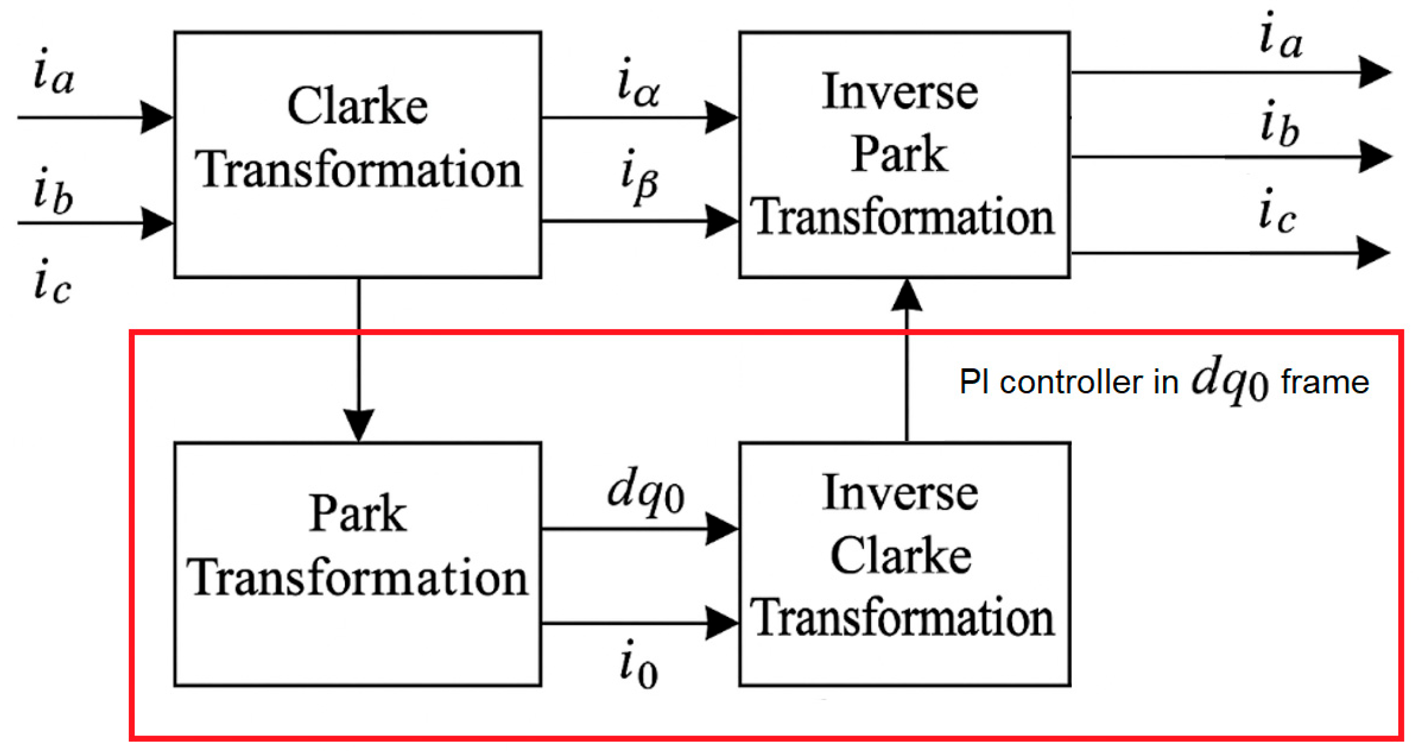
To implement the control strategy and to form the PWM control signals for the IGBT modules, a synchronous rotating reference frame (dq₀) was employed. This frame allows for the decoupling of the active and reactive components of the current, facilitating the implementation of PI-regulators with an improved dynamic response. The αβ reference frame was initially used as an intermediate stage via the Clarke transformation, followed by the Park transformation into the dq₀ domain. This approach enables effective current control under varying load and battery conditions. The reverse transformation is applied before signal generation for PWM modulation.

The visualization of the transformation structure is presented in Figure 6.

Real-time mathematical modeling provides a detailed analysis of the operation of the designed or tested device, as well as its operating modes, which allows optimizing the process of creating an experimental sample. The purpose of this work is to study and experimentally test the charging algorithms [52] of the traction battery of a passenger electric car. The use of mathematical modeling tools greatly facilitates this process. When constructing a mathematical model, a mathematical formalization of an object is necessary, and the connections and relations discovered and assumed in the device can be described using mathematical relations. The quality of the model determines the entire subsequent analysis of the object of this study, which is considered to be a charger integrated into the power circuit of a traction voltage inverter with an integrated charger based on the thyristor pulse control system (TPCS).

On the basis of specialized software, mathematical dependencies and relationships between them, a computer model has been formed, which provides the ability to set the required initial data, to calculate intermediate values and output parameters and to display the results for further analysis.

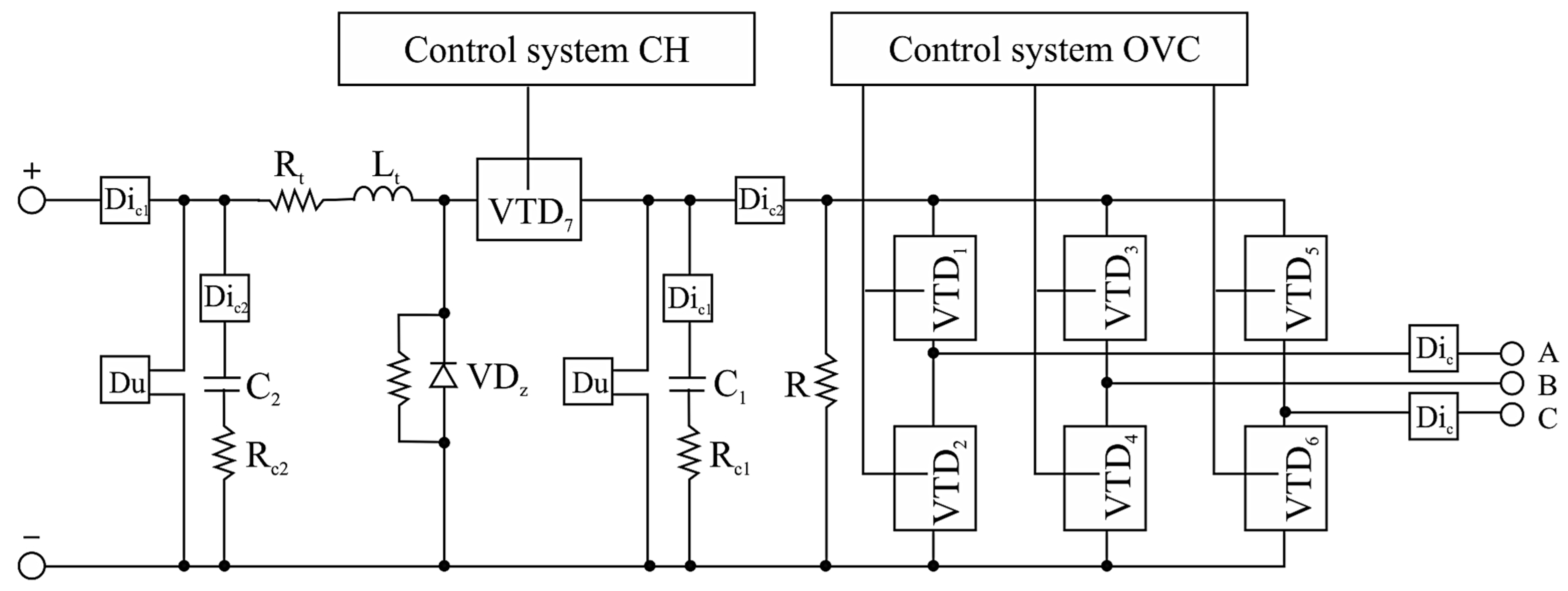
The substitution schemes and known dependencies described in [53,54] form the basis of the TPCS mathematical model. The basic electrical diagram of the power part of the device is presented in Figure 7 and reflects the features of the mathematical description of the components included in it. In the diagram, Control system CH is the control system of the TPCS and Control system OVC is the control system of the transistorized voltage converter.

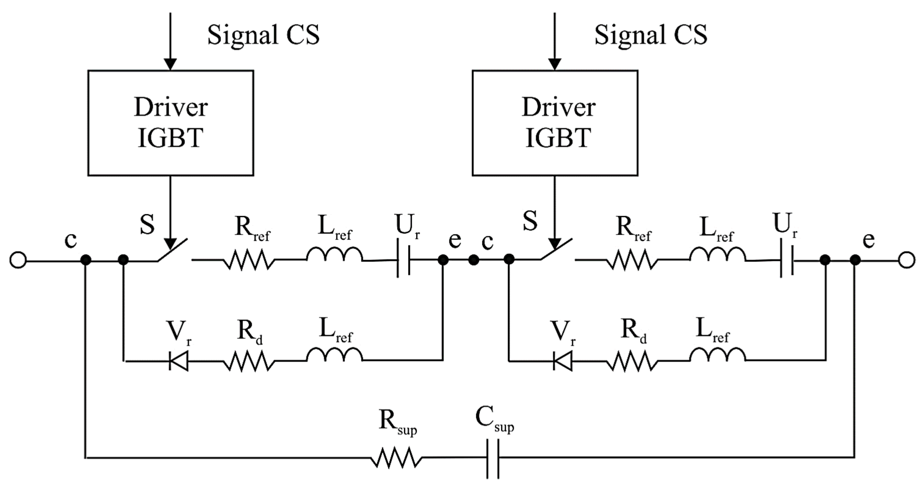
An insulated-gate bipolar transistor [55] included in the module (IGBT module) is considered as the main controllable element. The IGBT module replacement diagram is shown in Figure 8.

The Control Signal (CS) is fed to the IGBT driver, providing the impulse controls needed to control the state of the power switches. Ideal S switches implement the basic switching function, reproducing the on/off behavior of real power transistors. The model takes into account the resistance of the open R_ref channel of 0.014 Ω and the voltage drop (U_r) at an open collector–emitter junction equal to 1.7 V, which corresponds to the characteristics of the Infineon FS75R12KT4 transistor (Infineon Technologies AG, Neubiberg, Germany). For the adequate simulation of transient processes, the L_ref parasitic inductance of 28 nH is introduced, reflecting the dynamics of the current change at the moment of switching. A damper RC circuit with parameters of R = 4.7 Ohm and C = 470 nF is used to limit overvoltage and to suppress oscillatory processes at the output of the IGBT module, simulating the behavior of a snubber capacitor. The analog impact brings the power switch to the appropriate state, while time synchronization is observed and switching delays are minimized. At the same time, the typical delay value is no more than 800 ns. The charger control system is based on the generation of a control signal, described as a switching function that implements the on or off switching of the VT7 transistor (QuartzCom AG, Grenchen, Switzerland) depending on the value of the reference voltage. The mathematical implementation of the switching function depends on the current system parameters and PWM logic. The initial parameters include the charging current i_c, which varies from 0 to 50 A depending on the stage of charge and the control mode. The voltage of the traction battery (U_b) varies from 48.6 V (at the beginning of charging) to 50.4 V (at the end). The number of batteries (ns) is 14 in series for the experimental module. The maximum voltage of one battery (U_1max) is set at 3.6 V in accordance with the characteristics of lithium-ion NMC-type cells. The current control system implements a feedback loop for the measured battery current, which allows automatically adjusting the control signal and maintaining the charge current at the set level. The charging current is formed in accordance with the transfer function of the PI controller, which provides static error suppression and the accurate tracking of the given trajectory.

In the developed model of the charging system, the Control Signal (CS) is sent to the IGBT module driver, where logical control pulses are generated for idealized S switches, which implement the switching process in accordance with the pulse width modulation algorithm. The main losses in the open state are described by the resistance of the Ron channel and the voltage (Uf) to an open collector–emitter crossing. To take into account transient processes in switching, Lon inductance was introduced, which characterizes the dynamic behavior of the power cell. The damper RC circuit simulates the operation of a snubber capacitor, which provides the voltage slew rate limitation and the prevention of overvoltage in the power switch.

The driver’s function block converts logical commands into signals that correspond to the required switching law defined by the us(t) function, ensuring time synchronization and the correct generation of control pulse edges. Hence, a mathematical model of the key control can be represented through a switching function:

$$S(t)=\left\{\begin{array}{l}1,\hspace{0.17em}\hspace{0.17em}{u}_{\mathrm{ref}}(t)>u_{\mathrm{saw}}(t);\\ 0,\hspace{0.17em}\hspace{0.17em}{u}_{\mathrm{ref}}(t)\le u_{\mathrm{saw}}(t),\end{array}\right.$$

(1)

where $u_{\mathrm{ref}}(t)$ is the adjustable reference signal that determines the output current level and $u_{\mathrm{ref}}(t)$ is the sawtooth voltage generated by the PWM generator and described by the Fourier series:

$$u_{\mathrm{saw}}(t)={\displaystyle \sum _{n=1}^{\infty }\frac{2U_m}{n\pi }}\sin (2\pi n{f}_{\mathrm{ch}}t),$$

(2)

where $U_m$ is the amplitude of the reference signal and $f_{\mathrm{ch}}$ is the switching frequency.

The charger control system generates a u_ref(t) signal based on the set value of the charging current (i_c), the battery voltage (U_b), the number of ns cells connected in series and the maximum permissible voltage of one cell ($U_{1\max }$). The control signal is generated via a feedback channel in the form of a closed control system with PI control. The transfer function of the current regulator is presented in the classic form:

$$W_{\mathrm{PI}}(s)=k_p+{\displaystyle \frac{k_i}{s}},$$

(3)

where $k_p$ is the proportionality coefficient and $k_i$ is the integral coefficient.

Considering the required value of the charging current and the voltage limitation of the battery, the value of the reference signal of the task can be obtained in the form of:

$$i_{\mathrm{ref}}(t)=k_i(i_c(t)-i_b(t))+k_p{\displaystyle \underset{0}{\overset{t}{\int }}(i_c(\tau )-i_b(\tau ))d\tau .}$$

(4)

To increase the resistance to interference and the correct reproduction of dynamics, the circuit can be supplemented with the filtering of feedback signals, implemented through filtering links of the low-frequency LPF type:

$$H_{\mathrm{filter}}(s)={\displaystyle \frac{1}{1+s{T}_f}},$$

(5)

where T_f is the time constant of the filter.

Within the framework of the mathematical model of the battery, a modified Shepherd model is used, which provides an adequate description of the charging processes, taking into account the temperature and dynamic effects. The battery voltage during charging is described by the equation:

$$u_b(i)=E_0+K{\displaystyle \frac{Q}{Q-I_t}}i+A{e}^{-B{I}_t},$$

(6)

where E₀ is the initial EMF, K is the polarization coefficient, Q is the nominal capacitance, I_t is the stored capacitance, i is the current charging current and A, B are the empirical coefficients.

The temperature correction of the model is implemented through the dependence of the E₀, Ri and Q parameters on the temperature (T), for example:

$$E_0(T)=E_0+{\alpha }_T(T-T_{\mathrm{ref}}),$$

(7)

where α_T is the EMF temperature coefficient and T_ref is the base temperature.

Therefore, the proposed mathematical model of an integrated charger for an electric car includes the characteristics of the power part, switching algorithms and the dynamics of the thermal processes in the battery. This enables the more accurate modeling and implementation of effective charging strategies, including adaptive and intelligent ones.

The function $u_{\mathrm{ch}}^{*}(t)$ is an input signal and is described by the transfer equation:

$$u_{\mathrm{ch}}^{*}(t)=\left[((i_{\mathrm{c}}+i_{\mathrm{c}}\cdot k_u)-i)\cdot {\mu }_{{\mathrm{reg}}_i}\right]\cdot i_{\mathrm{c}}^{-1}+(1+k_u),$$

where $k_u$ is the coefficient determined by the existing current to stabilize the current voltage.

$$k_u=U_{1\max }\cdot {\mu }_{{\mathrm{reg}}_u}-{\displaystyle \frac{U_{\mathrm{b}}}{n_s}}\cdot {\mu }_{{\mathrm{reg}}_u},$$

(8)

where ${\mu }_{{\mathrm{reg}}_i}$ and ${\mu }_{{\mathrm{reg}}_u}$ are proportional–integral controllers that reduce errors in the values of the current and steady-state voltage. The function of a proportional–integral regulator ${\mu }_{\mathrm{reg}}(t)$ is defined as

$${\mu }_{\mathrm{p}\_i}(t)=k_i\cdot t+k_e\epsilon (t)$$

(9)

where $k_e\epsilon (t)$ is the function of the proportional coefficient; $k_i\cdot t$ is the integral component of the PI-regulator; $k_e$ is the proportionality coefficient; $k_i$ is the integral coefficient; $t$ is the current time; and ε(t) is the incoming signal.

The control signal for a pulse width modulation (PWM) controlled transistor switch [56] is determined by its switching:

$$f_{\mathrm{ch}}(t)=\mathrm{sign}\left(\mathrm{sign}\left(u_{\mathrm{ch}}^{*}(t)-u_{{\mathrm{ref}}_{\mathrm{ch}}}(t)\right)+1\right),$$

(10)

where $u_{{\mathrm{ref}}_{\mathrm{ch}}}$ is the value of the impulse voltage given in the form of a Fourier transform.

Hence:

$$u_{\mathrm{ref}\_\mathrm{ch}}(t)=-U_{m\_\mathrm{ref}\_\mathrm{ch}}\cdot {\pi }^{-1}\cdot {\displaystyle \sum _{k=1}^{\infty }\sin k(2\pi f_{\mathrm{ch}}t)\cdot k^{-1}}+0.5\cdot U_{m\_\mathrm{ref}\_\mathrm{ch}},$$

(11)

The value of the $U_{m\_\mathrm{ref}\_\mathrm{ch}}$ amplitude and the switching $f_{\mathrm{ch}}$ frequency is determined based on the optimal operating mode of the charger. The relationships in the mathematical model of the charger control system are reflected in the form of a structural diagram shown in Figure 9. The $U_{m\_\mathrm{ref}\_\mathrm{ch}}$ amplitude for a given $f_{\mathrm{ch}}$ frequency is selected for a given mode of operation of the charger.

To improve the quality of control, the circuit can be supplemented with filtering elements in the current and voltage feedback lines.

The traction battery, as an integral part of the traction and power equipment system of an electric car, is described using the method of the discharge and charging characteristics of the battery proposed by Shepherd [57] and modified by a number of authors [58,59]. The model proposed as part of the work, unlike the original method, takes into account the temperature modes of the battery operation.

The Shepherd equations for lithium-ion batteries are presented as:

• A bit function (I > 0):

$$U_{\mathrm{bd}}=E_0-K\cdot {\displaystyle \frac{Q}{Q-It}}\cdot i-K\cdot {\displaystyle \frac{Q}{Q-It}}\cdot It+A\cdot \exp (-B\cdot It),$$

(12)

• A charging function (I < 0):

$$U_{\mathrm{b}\mathrm{c}}=E_0-K\cdot \frac{Q}{It+0.1\cdot Q}\cdot i-K\cdot \frac{Q}{Q-It}\cdot It+A\cdot \exp (-B\cdot It),$$

(13)

where E₀ is the initial discharge/charge voltage (battery EMF), V; K is the polarization coefficient B/A·h; Q is the maximum battery capacity, A·h; i is the instantaneous value of the battery current, A; $It$ is the realizable capacity, including the initial battery state, A·h; and A and B are coefficients determined by the initial experimental characteristics of the battery in charge and discharge modes, A, A·h^–1.

In order to improve the accuracy and stability of the regulation in the conditions of the real operating modes of an electric vehicle, it is advisable to provide for the use of filtering elements in the current and voltage feedback lines in the structure of the control system [60]. These elements allow eliminating high-frequency noise that occurs when switching power switches and in the dynamics of the traction battery, thereby providing a more accurate generation of the control signal [61]. In a typical case, a low-pass filter with a transfer function of the following type is used:

$$H_{\mathrm{LPF}}(s)={\displaystyle \frac{1}{1+s{T}_f}},$$

(14)

where T_f is the filter time constant chosen based on the trade-off between interference suppression and system performance (e.g., T_f = 1.5×10^–3 s for an experimental bench).

The traction battery is considered as a key element of the traction and the energy system of an electric vehicle, determining the energy and thermal characteristics of the entire power chain. Its mathematical model is based on an extended version of Shepherd’s model, which makes it possible to describe the processes of charge and discharge, taking into account the nonlinear dependence of the voltage on the degree of the charge and temperature [62]. In contrast to the classical formulation, the model proposed in this paper is supplemented with a temperature correction of the parameters, which ensures the high adequacy of modeling in conditions close to real operation.

For the discharge mode (i > 0), the battery voltage is expressed as follows:

$$u_b(i)=E_0-K{\displaystyle \frac{Q}{Q-I_t}}i+A{e}^{-B{I}_t},$$

(15)

And for the charge mode (I < 0), a similar dependence is as follows:

$$u_b(i)=E_0+K{\displaystyle \frac{Q}{Q-I_t}}i+A{e}^{-B{I}_t},$$

(16)

where E₀ = 3.6 B is the initial voltage (battery EMF), K = 0.04 B/A·h is the polarization coefficient, Q = 10 A·h is the nominal capacity of the battery, i is the instantaneous current value, Tt is the accumulated charge and A = 0.1 B, B = 3 A·h^–1 are the empirical parameters obtained during the preliminary calibration on the bench.

Additionally, the temperature correction of the model parameters is implemented according to the expression:

$$E_0(T)=E_0+{\alpha }_T(T-T_{\mathrm{ref}}),$$

(17)

where αT = −2.5·10^–3 B/°C is the EMF temperature coefficient and T and T_ref = 25 °C are the current and nominal temperatures, respectively.

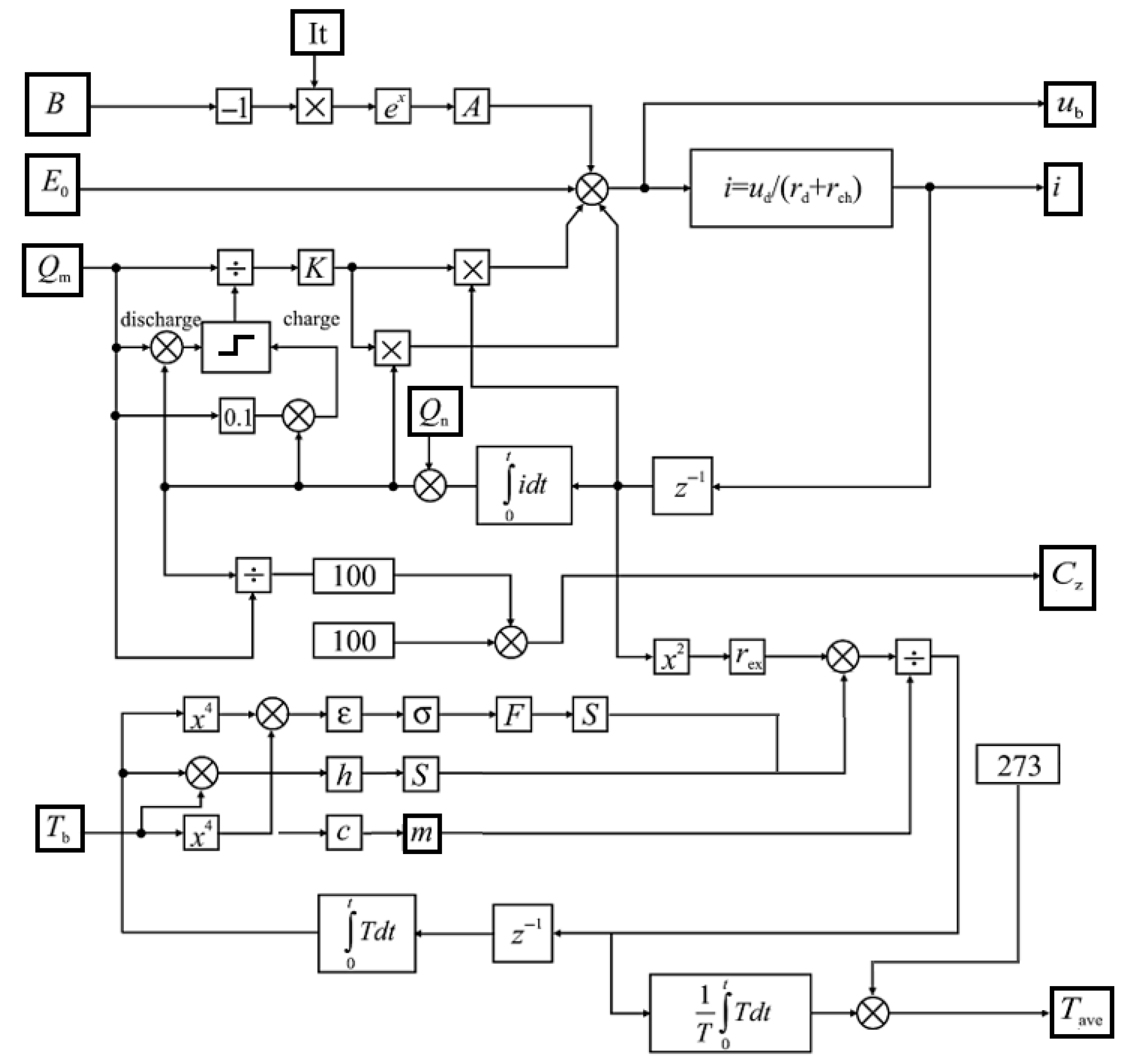
The relationship between the model parameters and the processes occurring in the battery is presented in the form of a structural diagram in Figure 10. This scheme serves as the basis for the implementation of the digital model in the MATLAB/Simulink environment, providing integration with control units and the ability to adapt to various modes of operation of an electric vehicle [63]. The use of the extended Shepherd model with temperature adaptation allows reliably reproducing the dynamics of the battery voltage during charging and discharging and analyzing the effect of thermal processes on the overall efficiency of the vehicle’s power system.

As part of a comprehensive model of the traction power supply system of an electric vehicle, the traction battery model (TAB) is formed, taking into account a number of engineering assumptions that provide a balance between realism and computational efficiency. One of the key assumptions is that the internal resistance of the battery will be constant throughout the charge and discharge cycles. For the simulated prototype, this resistance is $R_{\mathrm{int}}=\mathrm{0.015..0.022}$ Ohm and remains unchanged at currents of up to 60 A, which was confirmed during discharge tests with a current step of 10 A. This assumption simplifies the numerical implementation of the model and allows the stabilizing of the calculation in Simulink.

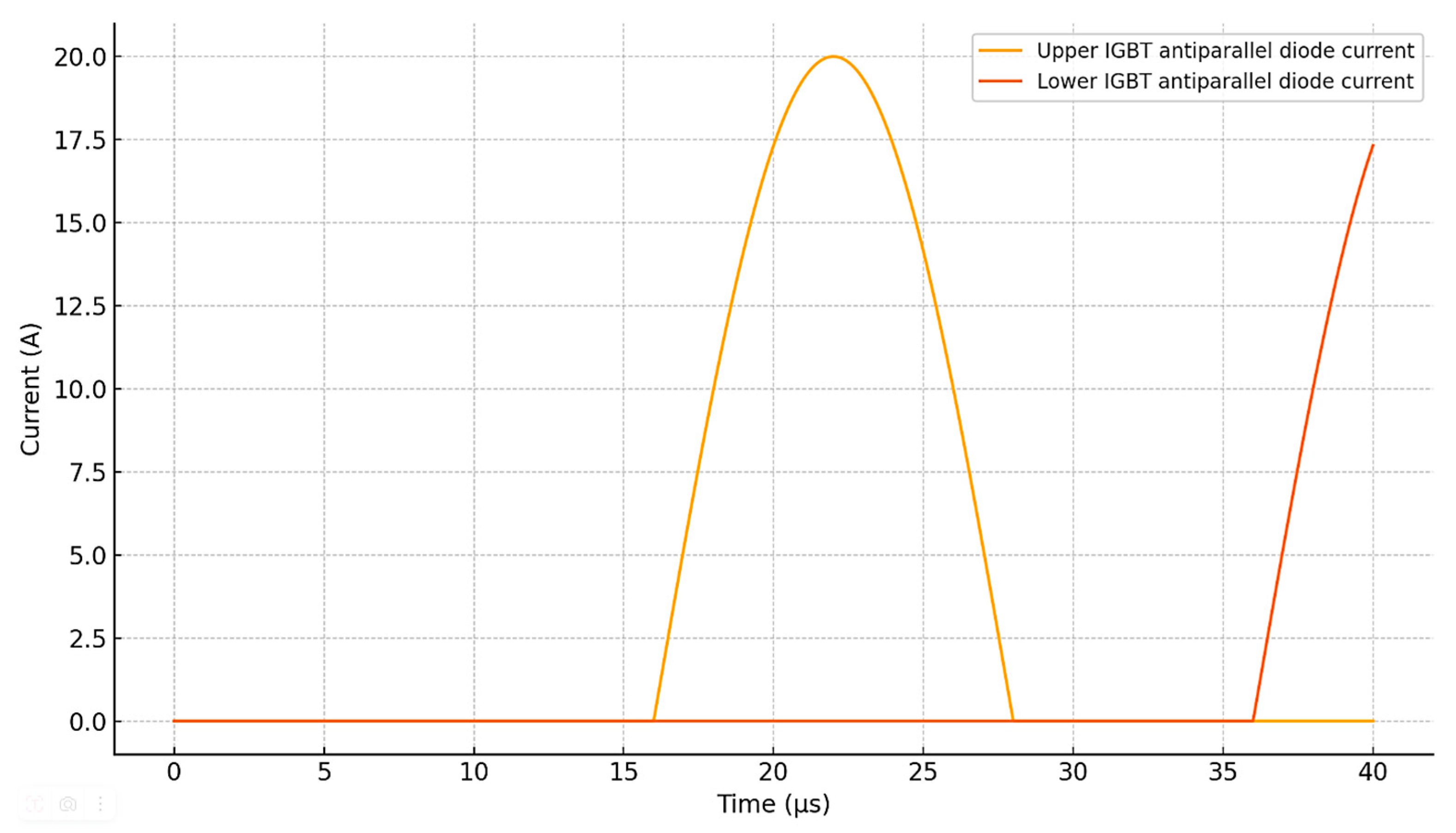
We illustrate the logic of the operation and switching of power devices and the redistribution of current between the semiconductors–Transistor–Diode Module, presented in Figure 8, while turning on/off. We gave the current graph through the power keys T1 and T2 (IGBT + Freewheeling Dior) for one period of PWM (current through the upper IGBT (or S1), current through the lower IGBT (or S2) and the current through their anti-parallel diodes at the time of one cycle at a frequency of 25–50 kHz) (Figure 11). The current schedule is in the damping RC-chain and parasitic inductance, which demonstrates peaks during switching and attenuation and explains the role of RC in restrictions (Figure 8) and the diagram of the total current at the time of switching to compare the total current with the battery current and the observation of pulsations.

The plot in Figure 11 illustrates the conduction of the freewheeling diodes when the corresponding IGBT transistor is turned off. The current peaks correspond to the commutation intervals, demonstrating how the diodes temporarily conduct the load current before the opposite transistor is activated. This behavior is critical for limiting voltage overshoots and ensuring correct energy circulation in the TPCS inverter (for one cycle of PWM at a frequency of 25 kHz, the period ~40 mks).

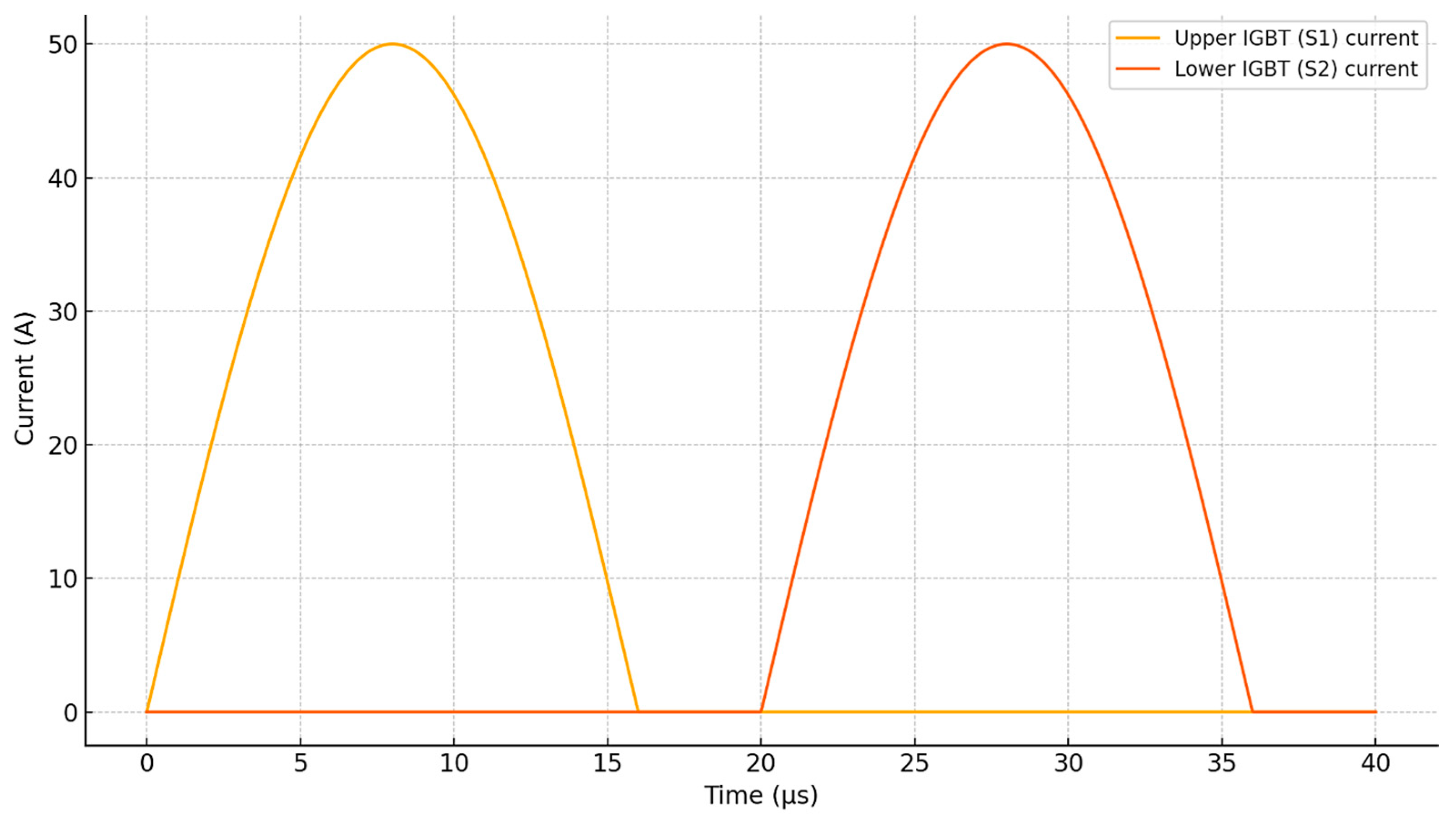
The plot in Figure 12 shows the conduction intervals of the main switching transistors. The upper IGBT conducts during the first half of the PWM cycle, while the lower IGBT conducts during the second half. The sinusoidal shape of the current reflects the modulation and transient switching dynamics. These curves are essential for understanding the distribution of conduction losses and thermal loading on the power devices (with a current amplitude of up to 50 A).

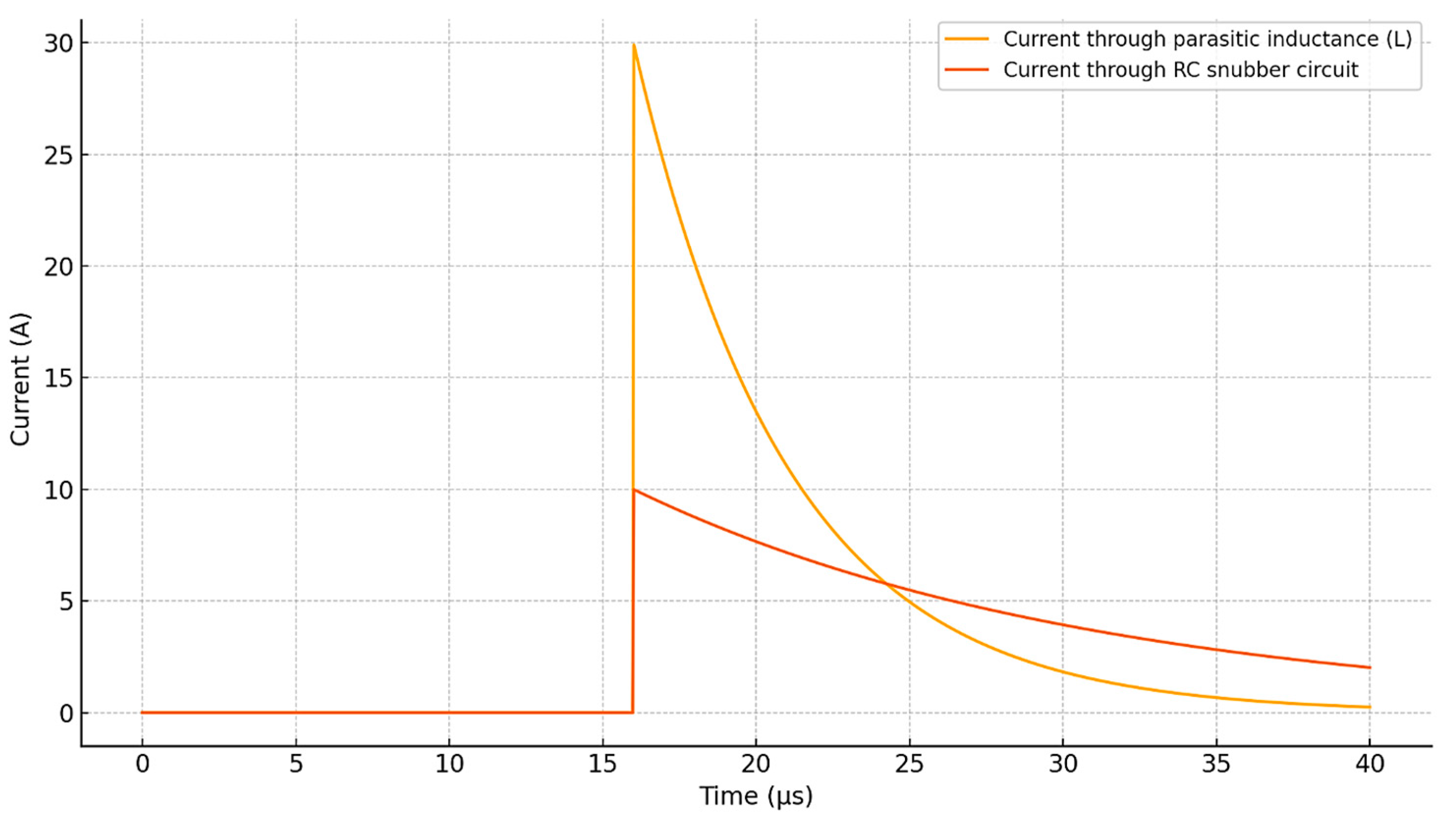
The plot in Figure 13 demonstrates a pronounced current spike through the parasitic inductance immediately after switching, followed by rapid decay within approximately 5 μs. Simultaneously, the RC snubber absorbs a portion of this transient energy, resulting in a smaller amplitude current that decays more gradually. This behavior confirms the role of the snubber circuit in damping overvoltage oscillations and protecting the IGBT modules from excessive voltage spikes. The plot in Figure 13 demonstrates a peak load when switching and the role of RC champions in absorption and smoothing outpances.

Thus, the presented waveforms (Figure 11, Figure 12 and Figure 13) clearly illustrate the switching behavior of the power devices and the redistribution of the current between the transistor and the diode during the on/off transitions. The peaks observed in the snubber current correspond to the voltage transients suppressed by the RC network. These data are providing a detailed visualization of current circulation within the TPCS model.

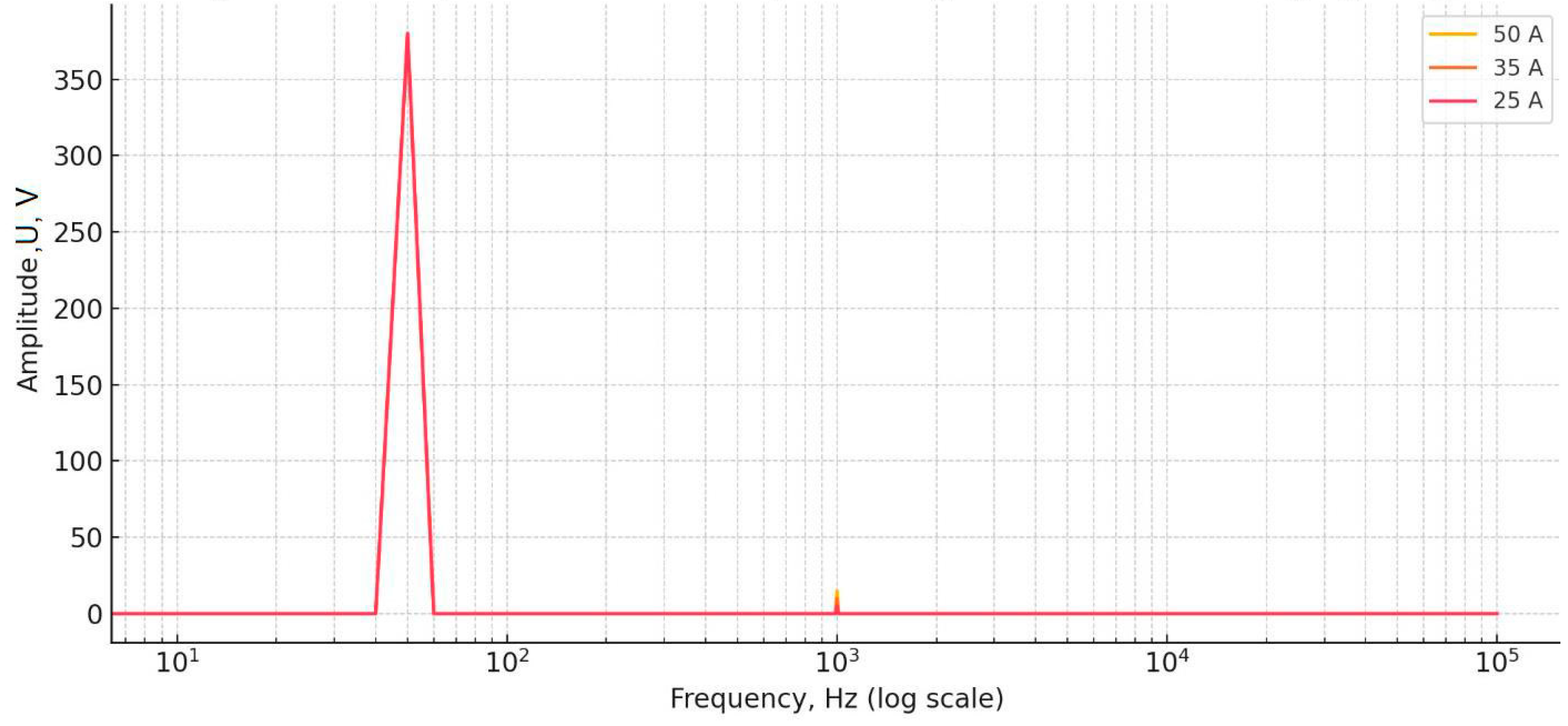
AC Waveform Analysis. In addition to the parameters of the DC accumulator, the voltage of the alternating current and the shape of the current wave at the output of the inverter was analyzed to evaluate the behavior of the switching and harmonic content at different stages of charging. As well as the frequency spectra of the output voltage of the alternating current for all three stages of charging. Figure 14 and Figure 15 show comparisons of the temporary area of the measured and simulated voltage of the alternating current and the shape of the current wavelengths during the first stage of charging (50 A). The model accurately reproduced the amplitude and the shape of the signals controlled by the PWM with an error of the square environment below 2%.

Figure 16 shows the frequency spectra of the output voltage of the alternating current for all three stages of charging. A decrease in the charging current led to a decrease in the amplitude of the fundamental harmonics at 10 kHz and the harmonics associated with them of a higher order, which confirms the ability of the model to capture the dynamic effects of switching. These results confirm the mathematical representation of the inverter and management strategies implemented in the modeling environment.

The electromotive force (EMF) of the battery (E₀), the polarization coefficient (K), as well as the empirical A and B parameters of the Shepherd model are obtained on the basis of the approximation of the discharge characteristics and are used to simulate charging. The battery voltage during charging is mathematically described by the expression:

$$u_b(i)=E_0+K{\displaystyle \frac{Q}{Q-I_t}}i+A{e}^{-B{I}_t},$$

(18)

where Q = 10 A·h is the nominal capacity, I_t is the accumulated charge and i is the instantaneous value of the charging current. The temperature effect on the EMF is considered by the dependence of the type:

$$E_0(T)=E_0+{\alpha }_T(T-T_{\mathrm{ref}}),$$

(19)

where α_T = −2.5·10^–3 B/°C, T_ref = 25 °C. At the same time, the capacitance is considered constant, the self-discharge processes are ignored due to their smallness in the time interval of up to 20 min (less than 0.3% of the capacity) and the memory effect is absent for lithium-ion cells. The temperature distribution is assumed to be uniform throughout the entire volume of the module, since according to the experimental data, the temperature difference between the cells did not exceed 2.1 °C. Thus, differential heat transfer equations can be abandoned.

The charger must be controlled to ensure that the charging modes comply with the permissible values of the current (not more than 50 A), voltage (up to 50.4 V) and temperature (not higher than 40 °C). The optimal charging algorithm should minimize the time of recharging under the following restrictions:

$$\left\{\begin{array}{l}i(t)\le i_{\max }=50\hspace{0.17em}\mathrm{A};\\ U_b(t)\le U_{\max }=50.4\hspace{0.17em}\mathrm{V};\\ T(t)\le T_{\max }=40\hspace{0.17em}°\mathrm{C}.\end{array}\right.$$

(20)

Known charging strategies include two-stage PT/PN, pulsed and accelerated algorithms, each of which has both advantages and limitations. For example, the PNPT/PN algorithm reduces Tch to 12 min, but leads to thermal degradation.

The developed three-stage charge algorithm (3PT/PN) is aimed at implementing a compromise between the speed and battery life. At each of the three stages, the charging current (Ich) decreases in response to reaching the limit voltage, implementing an adaptive strategy.

The realized capacitance was $Q_{\mathrm{real}}$ = 8.9 A·h, which is equivalent to 89% of the nominal, and the integral efficiency of the system is estimated as:

$$\eta ={\displaystyle \frac{Q_{\mathrm{real}}{U}_{\mathrm{avg}}}{{\displaystyle \underset{0}{\overset{t_{\mathrm{ch}}}{\int }}{P}_{\mathrm{in}}(t)dt}}}=85.5\%.$$

(21)

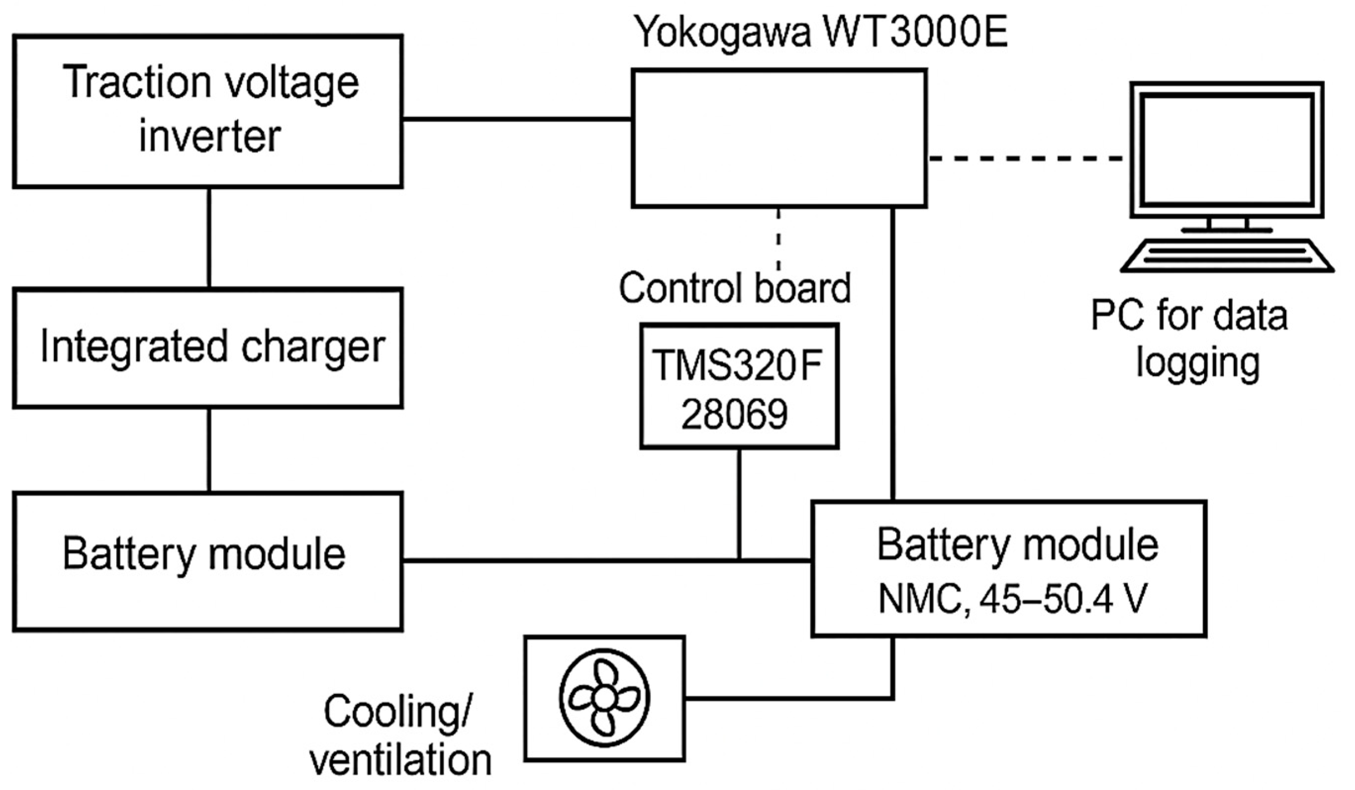
The initial conditions included the initial voltage (U_start = 48.6 V), the temperature (T_start = 18.5°C) and the duration of the stages (6.3, 5.8 and 4.9 min). The model was validated using data from Yokogawa WT3000E meters, which have an accuracy of a 0.02% current and 0.01% voltage. The $U_b^{\exp }(t),\hspace{0.17em}{I}_b^{\exp }(t),\hspace{0.17em}{U}_b^{\mathrm{mod}}(t),\hspace{0.17em}{I}_b^{\mathrm{mod}}(t)$ dependencies shown in Figure 11 and Figure 12 coincide in their amplitude, shape and time structure. This allows this model to be used to develop intelligent charge management systems, to predict thermal behavior and to optimize energy parameters in the power system of an electric vehicle.

The model parameters, including polarization coefficients and EMF values, are obtained on the basis of an approximation of the discharge characteristics and then applied without modification to calculate the charge modes. This assumption reduces the complexity of the model calibration while maintaining an acceptable accuracy of 2%. The capacity of the battery is assumed to be constant at the level of 10 Ah. It is considered unchanged depending on the amplitude of the charging current under current loads of up to 2 C. Spontaneous self-discharge processes, whose contribution to the energy balance of the battery at time intervals of less than 20 min is less than 0.3%, are also excluded from consideration. They do not have a significant impact on the accuracy of modeling. The memory effect characteristic of nickel–cadmium batteries is absent in the lithium-ion cells of the NMC type used and thus excluded. In addition, it is assumed that the temperature is evenly distributed throughout the entire volume of the battery module, which is confirmed by experimental measurements, where the temperature difference between the cells did not exceed 2.1 °C at all stages of charging. The introduced assumption of thermal homogeneity makes it possible to abandon complex thermal models and to use the simplified temperature correction of the model parameters.

Under charge conditions, the charger control system must adapt to the current state of the battery, taking into account the permissible values of the current, voltage and temperature. At the same time, the maximum current limit is 50 A, the voltage is controlled at 50.4 V and the temperature threshold is defined as 40 °C, which corresponds to the safe operating conditions for the lithium-ion cells used. The choice of the charging algorithm should take into account the performance and thermal stability, battery life, energy conversion efficiency and allowable charge time. Existing algorithms include simple two-stage strategies with a constant current and voltage, multi-stage, pulse and adaptive circuits. High-speed algorithms, such as PNPT/PN, reduce the charge time by up to 12–14 min, but are associated with the risk of the local overheating and accelerated degradation of active materials, which is confirmed by an increase in cell resistance after 100 cycles. On the contrary, gentle pulse methods with pauses can increase the service life by 15–20%, but require a charge time of more than 30 min. Therefore, a compromise between these extremes seems to be the most rational solution.

The three-stage charge algorithm (3PT/PN) developed in this paper is aimed at implementing such a compromise. It involves a gradual reduction in the charging current in response to critical voltage and temperature values, avoiding overheating and reducing the load on the internal structure of the battery. In the first phase, the charge is performed with a current of 50 A until a voltage of 49.98 V is reached, which corresponds to approximately 96% of the voltage of a full charge. The battery temperature does not exceed 29.3 °C, which is well below the critical level. In the second phase, the current is reduced to 35 A, while the voltage reaches 50.2 V. And in the third phase, the charge ends with a current of 25 A up to the level of 50.4 V. The duration of each stage is 6.3, 5.8 and 4.9 min, respectively; the total time of a full charge is 17 min. The capacity implemented in the experiment is 8.9 Ah, which is 89% of the rated capacity, while the measured efficiency value is 85.5% at an ambient temperature of 21 °C. These data confirm both the energy efficiency of the developed algorithm and its ability to provide a stable thermodynamic regime without going beyond safe temperature limits.

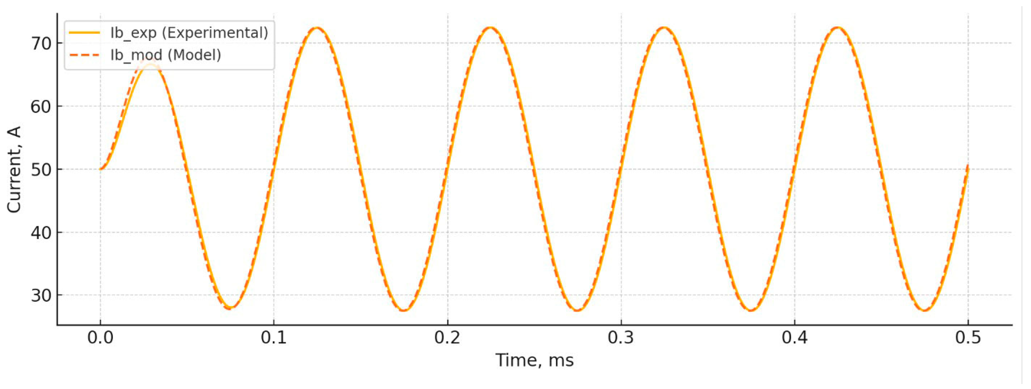
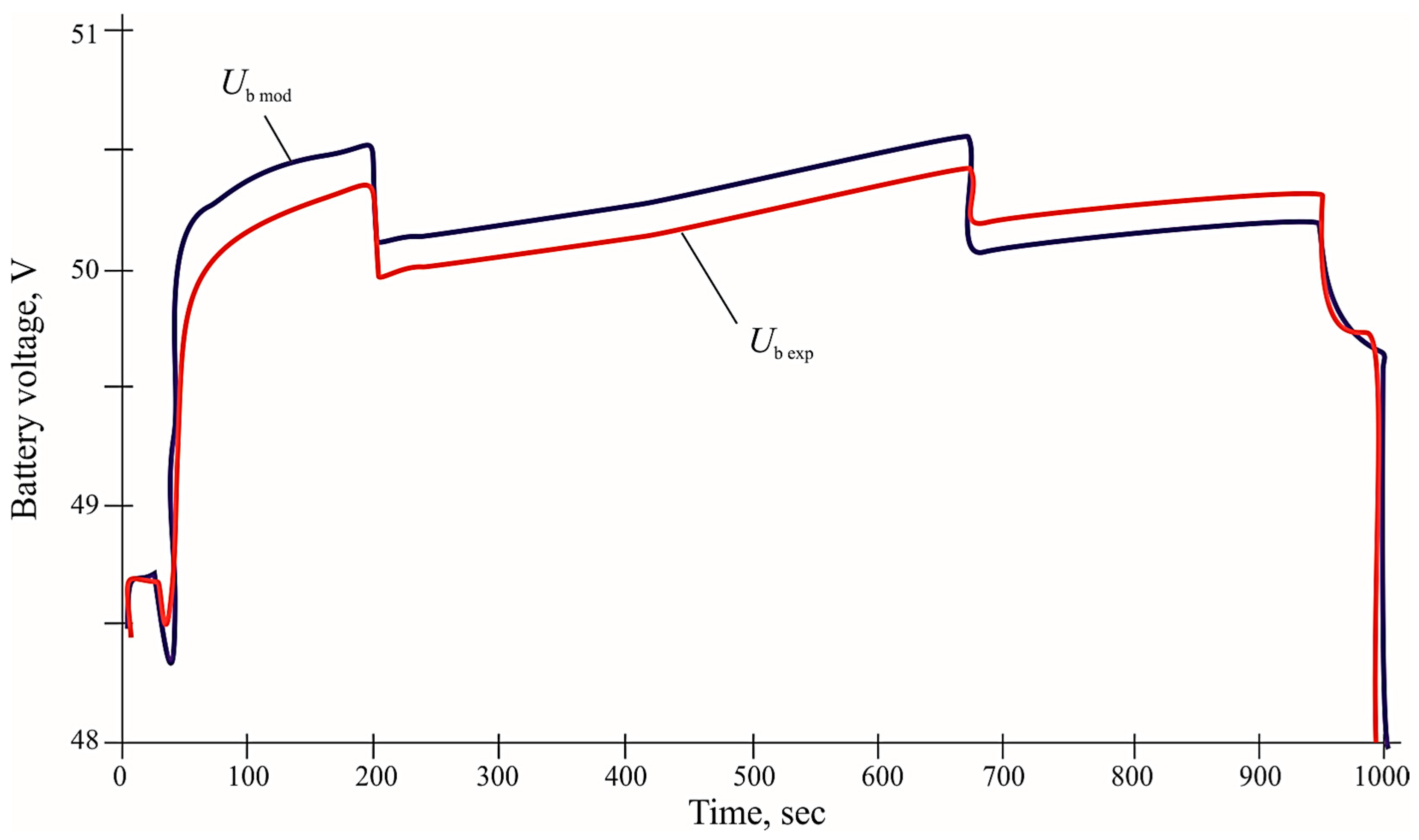
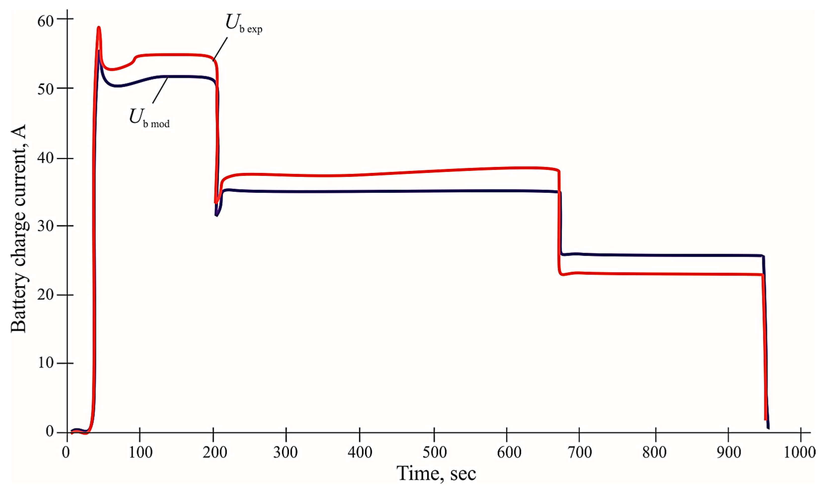
Experimental studies were conducted on a laboratory bench using a battery with a nominal voltage of 45 V and a maximum level of 50.4 V. The initial voltage of the module was 48.6 V, which corresponded to a state of charge of about 85% and the average temperature of the cells before charging was 18.5 °C. Accurate current and voltage measurements were made using Yokogawa WT3000E high-precision measuring instruments (Yokogawa Electric Corporation, Tokyo, Japan) with an error of less than 0.02%. The time that the voltage and current dependencies obtained during the experiment demonstrated a high degree of agreement with the results of modeling in the MATLAB/Simulink environment: the voltage deviation at the final stage did not exceed 0.71% and the current error was no more than 1%. Graphs of these dependencies are presented in Figure 12 and Figure 13, which compare the experimental curves (Ub _exp and Ib _exp) and the calculated trajectories generated by the complex model (Ub _mod and Ib _mod).

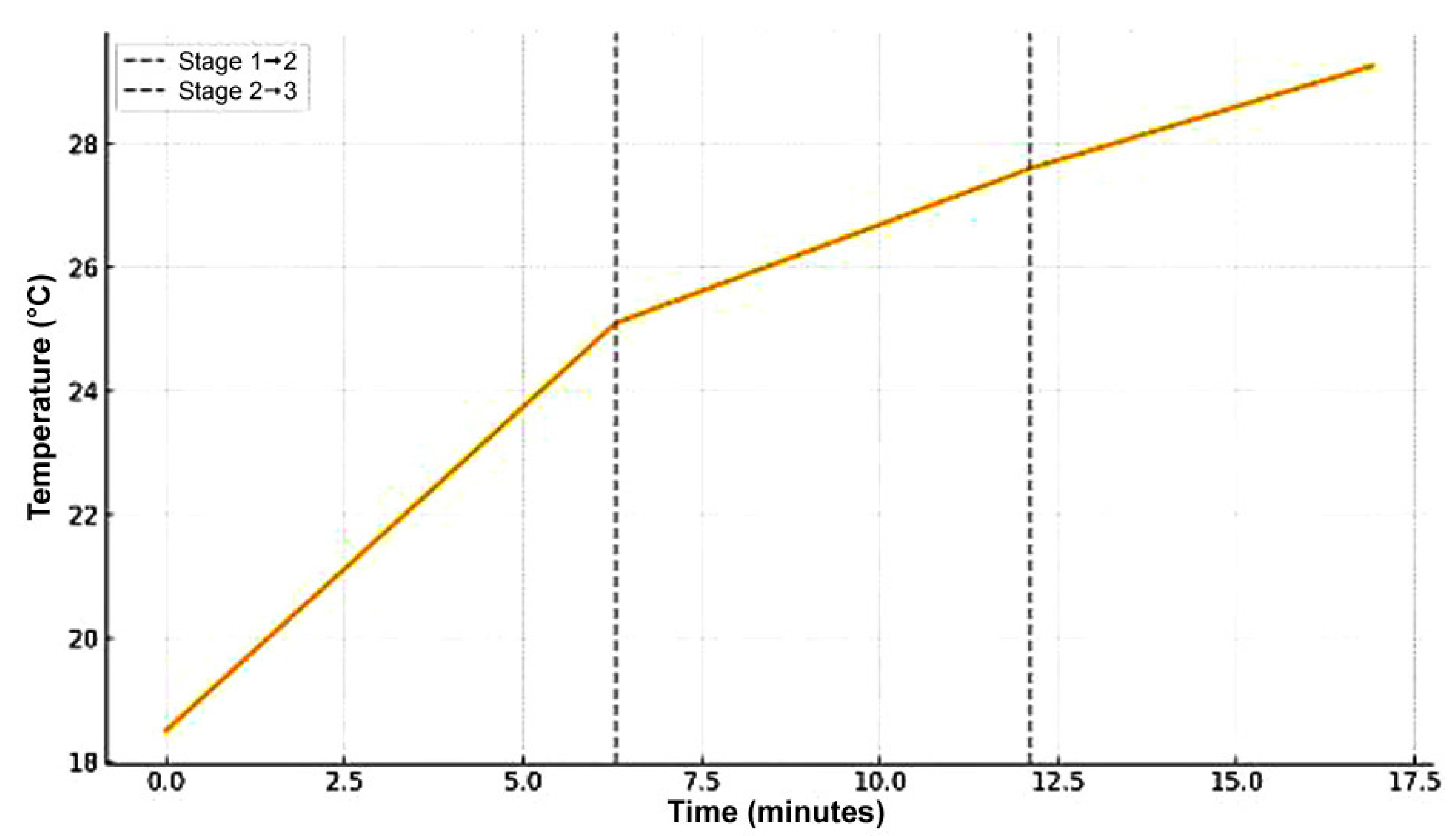
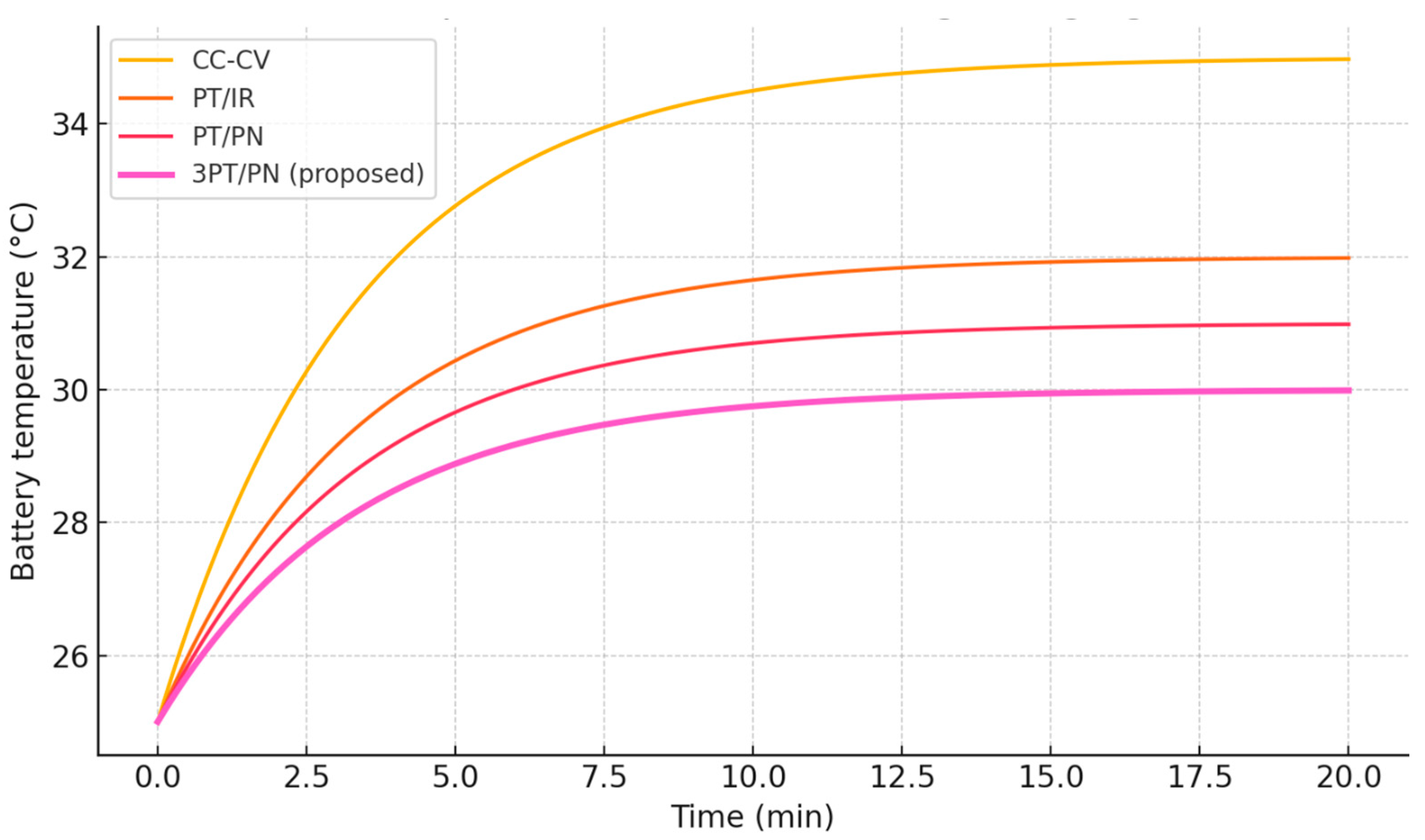
The effectiveness of the 3PT/PN charging algorithm in managing thermal dynamics was confirmed by real-time temperature measurements. Throughout the charging process, the battery temperature increased gradually from an initial value of 18.5 °C to a maximum of 29.3 °C at the end of the third stage. The temperature remained well below the critical threshold of 40 °C during all three phases of charging. The temperature rise was most prominent during the first stage (50 A), reaching approximately 25.1 °C by the end of the 6.3 min interval. During the second stage (35 A), the rate of the temperature increase slowed, with a final value of about 27.6 °C after 5.8 min. At the third stage (25 A), the temperature rose only slightly, stabilizing at 29.3 °C. These data demonstrate that the proposed charging algorithm maintains a safe thermal profile and confirms its suitability for practical applications. The corresponding temperature–time curve is presented in the Figure 17, where there are three stages of charging.

To provide a more objective and quantifiable assessment of the proposed algorithm’s benefits, we conducted a direct benchmarking experiment. The same charging hardware was used to charge the battery module under the classical PT/PN and the proposed 3PT/PN algorithms. The results are summarized in the table below and include comparative data on the charging time, realized capacity, thermal response and energy efficiency. The data clearly show that the 3PT/PN algorithm achieves a higher energy throughput in less time, with a significantly reduced thermal load. These advantages are critical for practical deployment in traction applications where compact cooling systems are employed. The comparison of the experimental results for PT/PN and 3PT/PN are presented in

Table 3. Experimental comparison of PT/PN and 3PT/PN charging strategies.

Parameter	PT/PN (Two-Stage)	3PT/PN (Proposed)
Total charging time	21 min	17 min
Capacity reached, Ah	8.7 Ah	8.9 Ah
Integral efficiency	83.2%	85.5%
Max. battery temperature, °C	34.8 °C	29.3 °C
Average battery temperature, °C	31.2 °C	26.7 °C
Max. charging current	50 A	50 A
Ambient temperature	21 °C	21 °C
Equipment used	The same (TPCS)	The same (TPCS)

Note: all the data were collected on the same lab setup using the same traction inverter charging module (TPCS), measured with Yokogawa WT3000E modules and DS18B20 temperature sensors (Yokogawa Electric Corporation, Tokyo, Japan).

.

Comparison with conventional charging methods: To assess the effectiveness of the proposed three-speed 3PT/PN algorithm, a comparative analysis is carried out with other charging methods in comparable conditions. Figure 18 shows graphics of changes in the degree of charge (SOC) of the battery element in time for 3PT/PN, the traditional two-stage CC-CV, a pulsed method with pauses (PT/IR) and a pulsed method with discharge pulses (PT/PN).

It can be seen that our 3PT/PN algorithm provides a comparable or faster achievement of complete charging compared to the classic CC-CV. For example, the charging time up to 100% at 3PT/PN is slightly less than that of CC-CV (on 20–25% faster) and close to the time of the pulsed method with discharge impulses, which is known for an accelerated charge. At the same time, 3PT/PN does not lead to a sharp increase in temperature. In Figure 18 shows the dynamics of heating the element when charging with different methods. The maximum temperature when using 3PT/PN is noticeably lower than with continuous CC-CV, especially at the stage of the main current. Impulse algorithms generally demonstrate a milder heat profile: alternating pauses or bites of discharge impulses gives the battery the time to take heat and reduce polarization effects. For example, curves show that by the end of charging, the temperature of the element at 3PT/PN by ~10° C is lower than with a two-stage method. This behavior is consistent with literary data: pulse charging is characterized by a lower heat load and less intensive old battery aging. Also, thanks to pauses/discharge impulses, the average internal resistance is reduced during charging, which reduces the heat release. In particular, the mode with the alternation of the charge (analogue of our 3PT/PN) in the experiments showed the smallest internal resistance and the shortest charging time among the tested protocols.

In general, the advantages of 3PT/PN can be clearly demonstrated based on the analysis of graphs in Figure 18. It is easy to notice that 3PT/PN provides faster charging, comparable to pulsed methods, with the moderate heating of the battery. A text analysis under the figures will emphasize that our algorithm combines the advantages of impulse techniques—high speed and effective depolarization—with temperature control. For example, 3PT/PN reaches a full charge faster than the standard CC-CV (by eliminating the delays in the phase of the dose), while the maximum temperature is lower by 10–15%. Thus, a comparative analysis convincingly shows the advantages of the proposed 3PT/PN algorithm over alternative approaches.

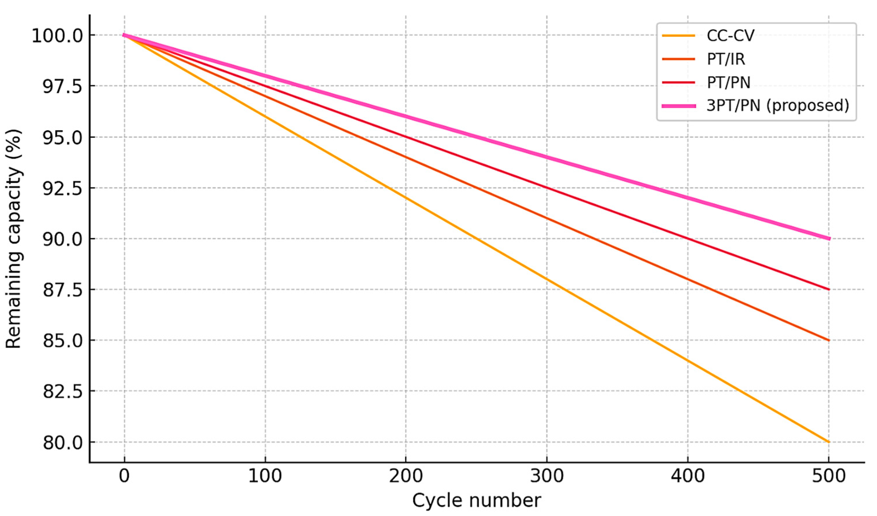
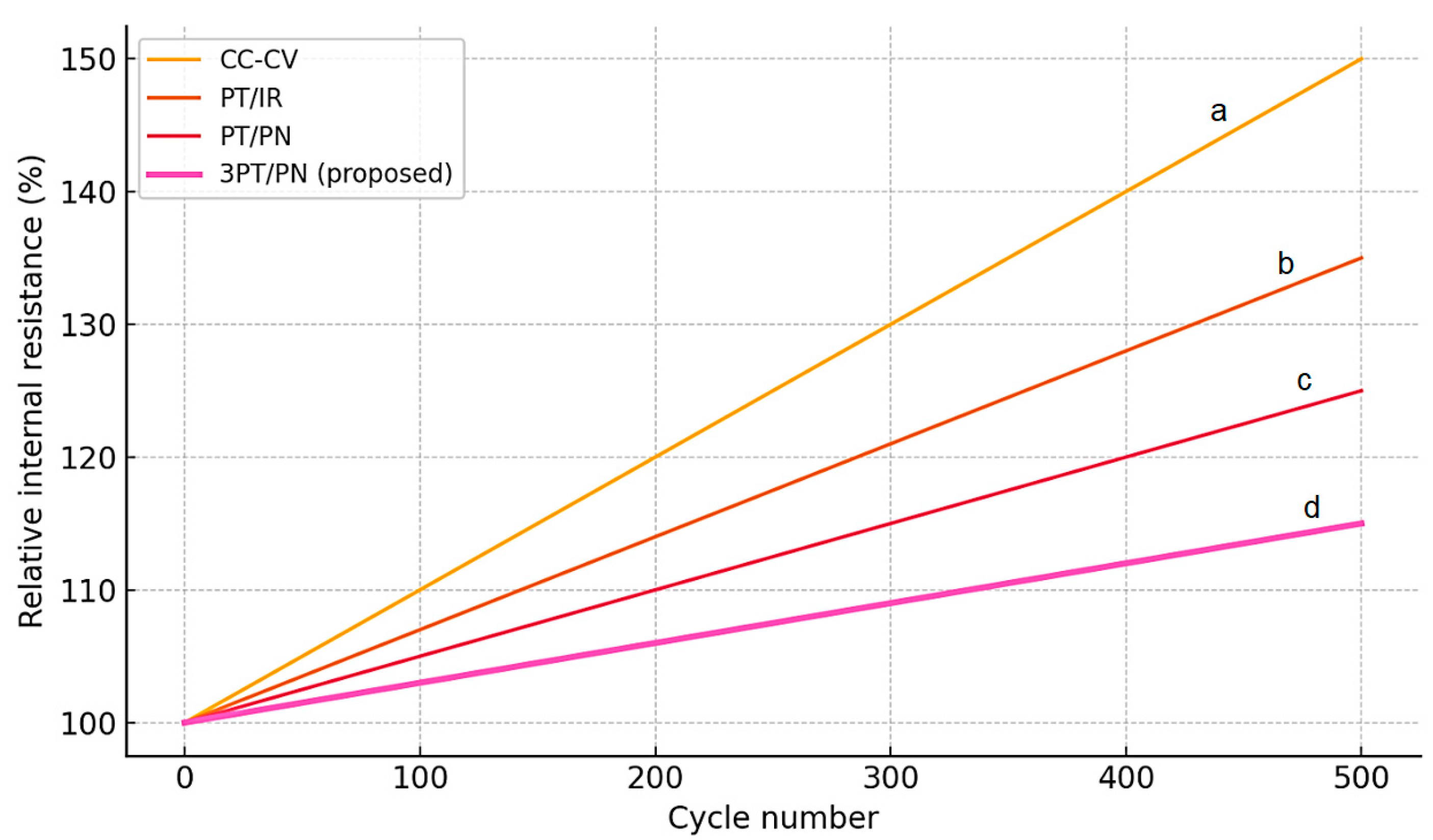
Cycle life simulation: Additionally, a long-term operation of the battery during the cycles is carried out in a charge–discharge for the 3PT/PN algorithm and the compared methods. The results are presented in Figure 19. The dependence of the internal resistance of the battery elements changes depending on the number of cycles for the same methods. You can observe how much faster the resistance is due to the degradation of the electrodes and the SEI with different algorithms. The graphic of Figure 19 shows a decrease in the relative capacity (Q/Q₀) depending on the number of cycles to 500. It can be seen that the battery charged according to the standard CC-CV protocol loses the capacity of all those that are fastest: already by 300, the cycle remains at 80% of the initial capacity. Impulse techniques demonstrate a slower degradation—for example, about 85% (PT/IR) and 88% (PT/PN) from Q₀ remains at 300 cycles. When using the 3PT/PN algorithm, the maintenance of the capacity is the best: even after 300–500 cycles, the relative capacity is higher than that of the rest (for example, 90% on the 300th cycle). These data indicate that our three-speed algorithm marks the battery life noticeably compared to the traditional two-stage charge. This is consistent with the research: for example, a high-frequency impulse charge can almost double the number of cycles to a loss of 20% of the capacity.

The graphics b and c of Figure 19 show a change in the internal resistance of the element during cyclizing. The initial value is normalized as 100%. It can be seen that the method of CC-CV R_INT grows the fastest—about 40–50% after 500 cycles (conditionally). Impulse algorithms slow down the increase in resistance: to the 500th cycle, an increase in 30% (PT/IR) and 20% (PT/PN). For the 3PT/PN algorithm, the resistance growth is minimal—about 10–15% for the same period. A lower increase in the internal resistance of the battery element in 3PT/PN indicates a lower worship of conductivity and a less intense increase in the passivation of electrodes. This corresponds to literary data, where the impulse charge reduces the growth rate of the impedance of the battery due to the uniform distribution of lithium and the reduction in the thickness of the interference layer.

The graphs in Figure 20 show the temperature evolution during the charging of the battery element when charging with different methods. There is a change in the maximum temperature of the battery when charging as it is aging. In all methods, there is a slight increase in temperature with the number of cycles (due to growth r_int and increasing heat generation). However, with algorithm 3PT/PN, the temperature growth rate is lower: to the 500th cycle, the maximum temperature rises slightly (for example, from 30 °C to 33 °C), while with CC-CV, it reaches 37 °C. The pulse regime with pauses/discharges also holds heating below the continuous method. Thus, the 3PT/PN not only initially less heat in the battery, but also prevents the increase in thermal peaks with the age of the battery.

Thus, the results of long-term modeling demonstrate the advantages of 3PT/PN: a slower decrease in the capacity and internal resistance growth means the extension of the battery resource. Our algorithm reduces degradation due to a gentler regime: alternating the charging stages reduces mechanical and chemical stresses in the electrodes. In particular, the avoidance of a long phase of a constant voltage (CV) prevents intense adverse reactions in the electrodes, which are characteristic of the standard CC-CV and accelerate aging. The impulse discharge pauses in 3PT/PN contribute to the destruction of passivating layers and the uniform redistribution of ions, which leads to a thin SEI and a smaller increase in resistance. In the aggregate, the presented graphs show that 3PT/PN is able to ensure durability that exceeds other charging methods.

Analysis of internal battery characteristics: An important advantage of the 3PT/PN algorithm is a beneficial effect on internal processes in the battery. The dynamics of the internal characteristics were analyzed—the growth of resistance, a change in the available capacity and a tendency towards lithium precipitation with different methods of charging, Figure 21. Graphic CC-CV in Figure 21 illustrates the growth of internal resistance as cyclical. The 3PT/PN algorithm demonstrates the minimum growth of internal resistance, which indicates a shorter increase in passivating layers (SEI) and a lower deterioration in the interfaces’ conductivity. On the contrary, with a standard CC-CV there is a thicker SEI and strong adverse reactions lead to a significant increase in resistance.

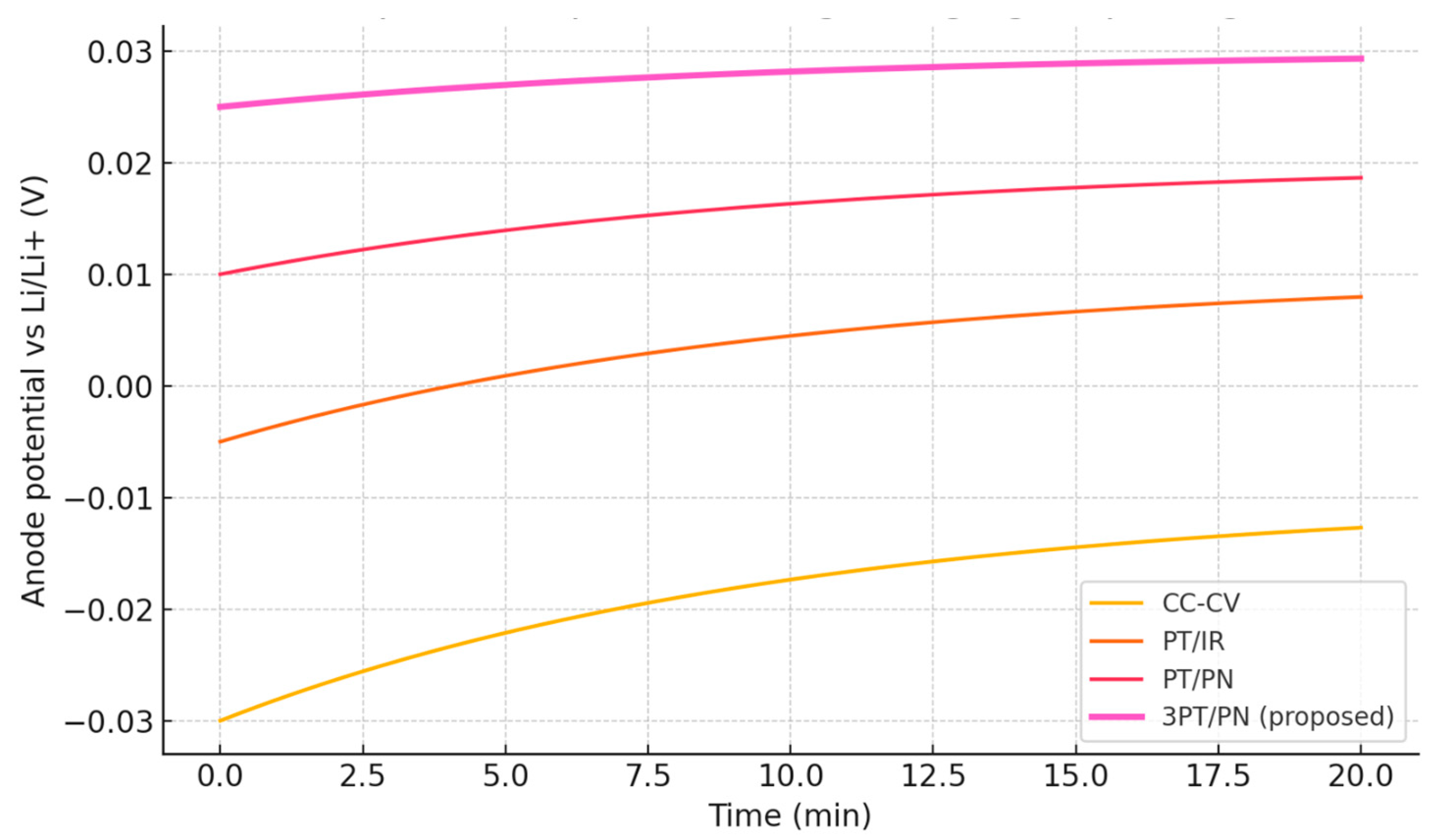
Figure 21 (graphics CC-CV and PT/IR) shows a decrease in the relative capacity of Q/Q₀, associated not only with the loss of active lithium, but also with the accumulation of “dead” lithium (besieged at the anode) and the degradation of the structure of the electrodes. It can be seen that by 300–500 cycles in CC-CV, the battery loses more of its capacity than with 3PT/PN. This is partially due to lithium precipitation: aggressive charging conditions (high current at the final stage without pauses) lead to the deposit of metal lithium on a graphite anode, especially with increased SOC and if the anode potential of Li/Li+ drops below 0 V. Impulse algorithms, especially with discharge impulses, effectively suppress Li-Plating. In our case, 3PT/PN includes phases that redistribute lithium ions and remove polarization, not allowing the anode to achieve critical overvoltage. Modeling shows that during a pulsed charge with high currents, periodic pauses/discharges align the concentration of LI+ at the surface of the anode, softening the drop in the anode potential and preventing lithium deposition. For example, after 300 cycles of a pulsed fast charge, the surface of the graphite anode remains clean, without metal lithium, while with a continuous charge, LI deposits are observed on the anode.

To illustrate this effect, graphic PT/PN in Figure 21 schematically compared the states of the anode after a long cyclic: in CC-CV, the thickened SEI and the precipitated LI areas (metal dendritic deposits) are visible, which leads to an increase in resistance and an irrevocable loss of lithium. When charging 3PT/PN, the SEI layer is thinner, the graphite structure is less damaged and lithium precipitation is absent. This algorithm, in fact, performs depolarization measures in the charging process—similarly to the well-known pulsed methods with discharge impulses that reduce the thickness of the SEI and prevent the growth of dendrites.

The inclusion of such an analysis in this article (graphics + description) will demonstrate to the reviewer that this work takes into account not only external parameters (temperature), but also the internal electrochemistry of the battery. The discussion can be placed in the Discussion section, linking the observed advantages of 3PT/PN with a decrease in the internal degradation processes. Thus, 3PT/PN slows down the formation of passivating layers and prevents lithium precipitation due to the regular removal of polarization. All this leads to the preservation of the capacity and a decrease in resistance growth over time.

For an indirect assessment of the reliability of the battery, a comparison of the lithium precipitation diagram showing the risk of Li-Plating was carried out, namely the schedule for changing the anode potential from time to charge with different methods. It is noted that with CC-CV, the anode potential (relative to Li/Li+) drops below the critical level at the end of the charging (which provokes lithium precipitation), while with an impulse or multi-stage charge, the potential is maintained above the danger threshold due to the pauses and redistribution of the charge. So, after comparing the state of the anode after many cycles—with a conventional charge—lithium dendrites/deposits and thick SEI are formed, with 3PT/PN, where the surface of the anode is “clean”, without metal lithium.

This study and additional analysis confirm the effectiveness of the proposed three-speed 3PT/PN algorithm. Compared to the traditional two-stage charge and pulsed methods, 3PT/PN allowed a reduction in the charging time and heat emission, providing a milder battery mode. Modeling long-term cycles showed a slowdown in the degradation processes: the 3PT/PN battery retains the capacity and low internal resistance much longer (by tens of percent better, as of 300–500 cycles) compared to conventional CC-CV. An analysis of internal processes showed that this algorithm minimizes the growth of the SEI and prevents lithium deposition on the anode, eliminating the causes of accelerated wear and safety risks. Thus, 3PT/PN combines the advantages of fast charging and sparing effects on the battery.

The results of this study are of practical value for the development of advanced chargers: the implementation of the 3PT/PN algorithm will help increase the resource of lithium-ion batteries and ensure their safer operation in electric transport and portable electronics.

In addition to analyzing the voltage and current profiles at the battery terminals, an extended study was conducted to investigate the behavior of the input alternating current (AC) parameters supplied to the traction voltage inverter with an integrated charger. The simulation and experimental validation covered the line voltage and current on the AC side of the power circuit during the active battery charging phases.

The input line voltage remained sinusoidal throughout the charging process, with a root mean square (RMS) value of 229–231 V in the experimental setup and 230 V in the simulation model. Slight fluctuations of ±1.5 V were observed due to dynamic load changes associated with the modulation of the charging current at different algorithmic stages (50 A, 35 A and 25 A). The peak voltage values reached approximately 325 V, with minimal distortion and total harmonic distortion (THD) below 3% in both measured and simulated waveforms.

The input AC current exhibited a non-sinusoidal profile due to the pulsed nature of the current drawn by the inverter during the charging process. The RMS current measured at the AC input was approximately 3.12 A during the first charging stage (50 A DC), decreasing to 2.25 A and 1.65 A during the second and third stages (35 A and 25 A DC, respectively). The simulated input currents closely matched these values, showing RMS deviations of less than 1.2% at each charging stage. The waveform contained characteristic switching-induced distortions with predominant low-frequency harmonics, accurately reproduced in the simulation through the detailed modeling of IGBT switching behavior and input LC filter components.

The temporal alignment of the voltage and current waveforms confirmed the correct phase relationship and realistic power factor of approximately 0.98 during steady-state operation. This close correspondence between simulated and experimental AC-side parameters provides further evidence of the adequacy of the developed mathematical model in terms of the output charging characteristics and in relation to the electromagnetic behavior of the system under real operating conditions (Figure 22 and Figure 23).

These results underline the comprehensive nature of the modeling approach used in this study, capturing the dynamics of the low-voltage DC output and high-voltage AC input sides. The model can, therefore, be effectively employed for the further optimization of energy efficiency, electromagnetic compatibility and predictive diagnostics of integrated charging systems.

The coincidence of characteristic points and the shape of the curves confirms the high adequacy of the model and allows asserting its applicability for the subsequent synthesis of intelligent control algorithms, assessment of thermal conditions and optimization of charging profiles in power supply systems of modern electric transport.

The results obtained in the experimental studies with the data of mathematical modeling were compared according to two main parameters: the value of the charging current and the voltage at the terminals of the battery module. The highest degree of convergence was observed when using the three-stage 3PT/PN charge algorithm, especially in steady-state operating modes, where the relative deviation between the experimental and calculated values did not exceed 1%. In particular, during the transition to the second stage of charge and during stabilization at the third stage, the average absolute voltage error was 0.34 V, which is equivalent to 0.68% at the nominal level of 50.4 V. At the same time, the current error was 0.48 A, which corresponds to 0.96% at a current of 50 A. These values confirm the high accuracy of the model in a steady mode of operation, especially in the intermediate stages of the charge where the parameters are stabilized.

Errors between the experimental and calculated results were analyzed using standard methods of a comparative assessment based on the relative deviation of modeling parameters from experimental values in percentage terms. The maximum voltage deviation in the implementation of the 3PT/PN algorithm was 0.71%, which corresponded to an absolute difference of 0.36 V with a fixed voltage value of 50.4 V. Similarly, in terms of the current, the maximum difference reached 0.5 A, which gave a relative deviation of exactly 1%. Significant deviations of more than 1% were observed only during the initial period of charging, during the first 0.8–1.2 s after the start of the current supply, as well as in the final interval, when the charge current dropped below 3 A. These errors are due to several factors, including the inertial response of the analog part of the control circuit to a rapid change in the error signal and a decrease in the accuracy of measurements in the low current range.

The reasons for these deviations are, first of all, delays in the actuation of the control system, which under experimental conditions average 850–950 ns, depending on the stage of charge. Especially pronounced deviations are observed during the transition between charging phases, when the control action must be corrected according to a predetermined voltage and temperature threshold. Additional discrepancies are due to the limitations of the Shepherd method used in the battery voltage simulation. Despite the fact that the modified model takes into account the temperature dependence and nonlinear change in polarization resistance, it does not always adequately reproduce the behavior of the battery in transient modes, where significant current gradients (up to 20 A/s) cause a redistribution of potentials at the interface of the electrodes and the electrolyte. In the simplified model, such effects are expressed as local voltage peaks or drops, which do not find direct correspondence in the experimental curves.

Nevertheless, the obtained results unequivocally confirm the correctness and adequacy of the proposed mathematical model applied to the analysis of the charging mode of the traction battery of an electric car.

It is important to clarify that in the current implementation, the term “adaptive” can be referred to the algorithm’s real-time responsiveness to the measured battery voltage and temperature rather than to predictive or learning-based control strategies. The three-stage current regulation is governed by threshold-based logic, where transitions occur upon reaching predefined voltage levels, subject to additional temperature constraints to ensure thermal safety. Although these thresholds are fixed, the system responds dynamically to the actual condition of the battery during operation. While this does not constitute a fully adaptive control system in the strict sense (e.g., including SoC estimation or predictive control), it represents a practical and robust solution within the constraints of embedded hardware and computational simplicity. Future work may involve the integration of advanced control approaches, such as model predictive control (MPC), fuzzy logic or reinforcement learning, to enable more sophisticated optimization based on the real-time estimation of the state of charge (SoC) and state of health (SoH).

The model successfully reproduces steady-state and transient modes of the charger, including the response to changes in the current, voltage and temperature, as well as the dynamics of recovery processes when switching between charge stages. This makes it suitable for engineering calculations and the further optimization of the TPCS structural diagram when creating new prototype charging systems. The model provides the ability to test control algorithms, including classic two-stage and intelligent methods focused on minimizing energy losses and increasing the battery life. During the pilot test, the functional and energy characteristics of the experimental sample of the integrated charger based on the traction inverter were confirmed. In addition, the model allows visualizing complex transients in the power components of the system and the shape of the voltage and current curves in the switching zones. This is often difficult in real experiments due to the limitation of the frequency of registration or access to the internal elements of the circuit. In light of this, the developed approach can be effectively used in the tasks of the digital twin of electric vehicle charging modules and within the framework of the intelligent control of charging and thermal stabilization modes.

In the course of the performed work, the task of the comprehensive study of charging a traction lithium-ion battery of a passenger electric car was successfully achieved using the mathematical modeling and experimental verification of the results obtained. The created mathematical model made it possible to describe with high accuracy the dynamic and stationary processes occurring in the system of a charger integrated into the power circuit of a traction voltage inverter [64]. On the basis of this model, algorithms for controlling the charging process were developed, including the original three-stage 3PT/PN algorithm, focused on increasing the rate of replenishment of the battery energy while ensuring its safe and durable operation. The implementation of the experimental sample of the charger and its subsequent tests confirmed the correctness of the developed models and algorithms and proved the possibility of their use in real operating conditions of electric vehicles.

In particular, the maximum error in modeling the voltage of the battery module during charging was only 0.71%, which indicates the high accuracy of the constructed mathematical model. The error in modeling the charge current using the 3PT/PN algorithm did not exceed 1%, which confirms the adequacy of the applied mathematical dependencies and the correctness of the parameterization control systems. When implementing the three-stage charge algorithm, specific parameters were recorded: the current of the first stage of charging was 50 A, the current of the second stage was reduced to 35 A and then the current was maintained at the level of 25 A at the third stage. The criterion for the transition between the stages was the achievement of the voltage of the battery module of 50.4 V. The initial voltage of the discharged battery module before charging was 48.6 V, which corresponded to the state of charge of about 85%. During the charging process, a realized capacity of 8.9 Ah was achieved, and the integral efficiency [65] of the process was 85.5%, which indicates the high energy efficiency of the developed charger. Temperature control showed the stability of the thermal regime of the battery module throughout the entire charging process, which was especially important for extending the service life of lithium-ion batteries [66].

Summarizing the prospects of the conducted work, it should be noted that the developed mathematical model and experimental technique allowed the reproduction of the charging process in a wide range of modes and the optimization of it in order to improve the performance characteristics of the batteries.

4. Conclusions

The results of the studies have confirmed the high efficiency of the developed integrated charger based on a traction voltage inverter and the proposed three-stage charge algorithm (3PT/PN). The implemented structure of the charger has made it possible to reduce the total charging time and to increase the energy efficiency of the process. During the charging of the traction lithium-ion battery at an initial voltage of 48.6 V and an average temperature of 18.5 °C, a realized capacity of 8.9 Ah has been achieved. Temperature control throughout the process has demonstrated a stable thermal environment that stays within safe boundaries, which is critical for extending the battery life.

A comparative analysis of the data obtained as a result of mathematical modeling and experimental measurements has shown a high degree of compliance: the maximum error of modeling the voltage on the battery module was 0.71% and the current did not exceed 1%. This proves the reliability of the constructed mathematical model, including the influence of thermal effects and parameters of the control system links. This level of accuracy allows the model to be used to optimize charge modes in real operating conditions of electric vehicles.

The 3PT/PN algorithm has shown good results in terms of the charge rate and reducing the thermal and electrical stress of batteries. Charging currents of 50, 35 and 25 A in three successive stages have made it possible to achieve the required voltage level of 50.4 V without going beyond the temperature limits and without signs of overcharging. The use of this algorithm can be recommended as a universal solution for electric vehicles focused on frequent and intensive use, including urban.

Furthermore, the comparative analysis of the AC voltage and current waveforms demonstrated high fidelity between experimental measurements and model predictions, confirming the accuracy of the PWM control and the dynamic response of the charger.

The developed methodology, involving the construction of the mathematical model, its verification and the experimental implementation of the system, can serve as the basis for further research in the field of intelligent charge management, the adaptation of charging algorithms to the state of the battery and improving the overall energy efficiency of the transport system.

As a direction for future work, the integration of real-time battery diagnostics and predictive control strategies is foreseen. This may include algorithms that estimate the SoC and SoH online and adjust the charging current dynamically, further enhancing the adaptability and efficiency of the system.