Safety–Efficiency Balanced Navigation for Unmanned Tracked Vehicles in Uneven Terrain Using Prior-Based Ensemble Deep Reinforcement Learning

Abstract

This paper proposes a novel navigation approach for Unmanned Tracked Vehicles (UTVs) using prior-based ensemble deep reinforcement learning, which fuses the policy of the ensemble Deep Reinforcement Learning (DRL) and Dynamic Window Approach (DWA) to enhance both exploration efficiency and deployment safety in unstructured off-road environments. First, by integrating kinematic analysis, we introduce a novel state and an action space that account for rugged terrain features and track–ground interactions. Local elevation information and vehicle pose changes over consecutive time steps are used as inputs to the DRL model, enabling the UTVs to implicitly learn policies for safe navigation in complex terrains while minimizing the impact of slipping disturbances. Then, we introduce an ensemble Soft Actor–Critic (SAC) learning framework, which introduces the DWA as a behavioral prior, referred to as the SAC-based Hybrid Policy (SAC-HP). Ensemble SAC uses multiple policy networks to effectively reduce the variance of DRL outputs. We combine the DRL actions with the DWA method by reconstructing the hybrid Gaussian distribution of both. Experimental results indicate that the proposed SAC-HP converges faster than traditional SAC models, which enables efficient large-scale navigation tasks. Additionally, a penalty term in the reward function about energy optimization is proposed to reduce velocity oscillations, ensuring fast convergence and smooth robot movement. Scenarios with obstacles and rugged terrain have been considered to prove the SAC-HP’s efficiency, robustness, and smoothness when compared with the state of the art.

1. Introduction

Unmanned Tracked Vehicles (UTVs) play a pivotal role in construction engineering, search and rescue missions, and planetary exploration tasks due to their exceptional ability to move over unstructured terrains [1,2,3]. In real-world off-road exploration, to ensure safety and stability during navigation, UTVs are required to make decisions automatically using the collected real-time environmental information [4].

In recent years, DRL techniques have contributed greatly to solving complex non-linear problems in autonomous planning and decision making [5,6]. For instance, researchers have proposed dueling double deep Q-networks with prioritized experience replay (D3QN-PER) to enhance dynamic path planning performance by balancing exploration and exploitation more effectively [7]. Maoudj and Hentout [8] refined traditional Q-learning via new reward functions and state–action selection strategies to speed up convergence. Zhou et al. [9] tackled multiagent path planning under high risk by employing dual deep Q-networks that discretize the environment and separate action selection from evaluation, enhancing convergence speed and inter-agent collaboration. Moreover, hybrid methods merge deep reinforcement learning with external optimization, such as immune-based strategies [10], sum-tree prioritized experience replay [11] or heuristic algorithms [12] to ensure safer routes, shorter travel distances, and better path quality, demonstrating improved adaptability in unknown or dynamic environments. To enable the robots to move in off-road environments, multidimensional sensor data, including the global elevation map and the robot pose, are used as input to learn planning policies [13,14].

However, the global elevation map is unavailable in unknown off-road environments, making it more suitable to use local sensing technology during exploration. Zhang et al. [15] employed deep reinforcement learning to process raw sensor data for local navigation, enabling reliable obstacle avoidance in disaster-like environments without prior terrain knowledge. Weerakoon et al. [16] combined a cost map and an attention mechanism to highlight unstable zones in the elevation map, filter out risky paths, and ensure safe and efficient routes, which improved success rates on uneven outdoor terrain. Nguyen et al. [17] introduced a multimodal network that fuses RGB images, point clouds, and laser data, effectively handling challenging visuals and structures in collapsed or cave-like settings and enhancing navigation accuracy and stability.

Moreover, energy efficiency is a growing priority in intelligent transportation and autonomous navigation systems. Viadero-Monasterio et al. [18] proposed a traffic signal optimization framework that improves energy consumption by adapting to heterogeneous vehicle powertrains and driver preferences. Their method achieved up to 9.67% energy savings for diesel vehicles by customizing velocity profiles and acceleration behaviors. Although their work focuses on signalized intersection traffic, the idea of embedding energy-aware policy adaptation inspires us to explore lightweight reward shaping strategies. In this study, we introduce a velocity-stabilizing term in the reward to indirectly suppress excessive acceleration and promote smoother, energy-conscious navigation.

Apart from the abovementioned problem, the sample efficiency and deployment safety of DRL limit the navigation performance [19]. In terms of the sample efficiency, especially in cases with sparse rewards, DRL agents might converge to local optima, thereby hindering the learning of optimal policies [20]. Due to the black box nature of deep networks, DRL is unable to handle hard constraints effectively, which limits the generalization of the model and increases the difficulty of deployment safety [6]. These two problems can be alleviated by integrating prior knowledge using functional regularization [21,22].

This paper proposes an end-to-end DRL-based planner for real-time autonomous motion planning of UTVs on unknown rugged terrains. To enhance the training efficiency of UTVs and improve its adaptability in unknown environments, a prior-based ensemble learning framework, called SAC-based Hybrid Policy (SAC-HP), is introduced. The main contributions of this paper are as follows:

• This paper proposes a novel action and state space considering terrains and disturbances from the environment, which allows the UTVs to autonomously learn how to traverse on continuous rugged terrains with collision avoidance, as well as mitigate the effects of track slip problems without an explicit model.
• This paper introduces a comprehensive reward function considering obstacle avoidance, safe navigation, and energy optimization. Additionally, a novel optimization metric based on off-road environmental characteristics is proposed to enhance the algorithm’s robustness in complex environments. This reward function enables a shorter and faster exploration with smooth movement.
• To address the issues of low exploration efficiency and deployment safety in traditional DRL-based methods, we propose an ensemble Soft Actor–Critic (SAC) learning framework, which introduces the Dynamic Window Approach (DWA) as a behavioral prior, called SAC-based Hybrid Policy (SAC-HP). We combine the DRL actions with the DWA method by reconstructing the hybrid Gaussian distribution of both. This method employs a suboptimal policy to accelerate learning while still allowing the final policy to discover the optimal behaviors.

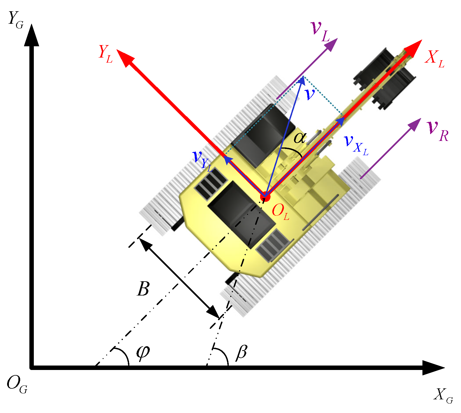
Notations: In this article, several symbols and variables are used, which are defined in

Table 1. Notation.

Variable	Description
r	Radius of the track drive sprocket.
$\mathit{\eta }$	UTV’s attitude.
x	The horizontal coordinate of the UTV center.
y	The vertical coordinate of the UTV center.
$\phi$	The yaw angle of UTV.
${\omega }_L$	Angular velocities of the left track drive sprockets.
${\omega }_R$	Angular velocities of the right track drive sprockets.
$v_L$	The forward velocities of the left tracks.
$v_R$	The forward velocities of the right tracks.
${\zeta }_L$	The slip rates of the left tracks.
${\zeta }_R$	The slip rates of the right tracks.
$\mathit{V}$	The UTV’s linear velocity vector.
$\alpha$	Sideslip angle.
$\mathit{s}$	State space.
$\mathit{a}$	Action space.
R	Reward function.
${\mathit{\chi }}_{tar}$	Target position state.
${\mathit{\chi }}_{obs}$	Obstacle position state.
${\mathit{\chi }}_{ele}$	Local elevation information.
${\mathit{\chi }}_{trans}$	UTV’s attitude change.
$X^G$	The horizontal coordinate in the global coordinate system.
$Y^G$	The vertical coordinate in the global coordinate system.
$X^L$	The horizontal coordinate in the local coordinate system.
$Y^L$	The vertical coordinate in the local coordinate system.
$d_i$	The closest obstacle distance in the i-th segment.
$P_r$	The position of the UTV.
$P_g$	The position of the target.
${\epsilon }_{col}$	Boundary of collision.
${\epsilon }_{safe}$	Boundary of safe.
$d_{goal}$	Boundary of goal.
$d_{near}$	Goal boundary threshold for positive reward.
$d_{max}$	Maximum scanning range of sensor.
N	Number of separated intervals within the sensor reading.
M	Elevation grid range.
N	Elevation grid size.
$\tau$	Number of samples used for linear velocity averaging.
${\pi }_{RL}$	The DRL policy.
${\pi }_{prior}$	The prior policy.
${\pi }_{hybrid}$	The hybrid policy.
$\mu$	The mean value.
$\sigma$	The variance value.
K	The number of ensembles of DRL agents.

. Note that the bold variables in this paper represent vectors and matrices.

2. Preliminaries

2.1. Kinematics Analysis

As shown in Figure 1, the robot’s motion is represented by a global coordinate system ($X_G{O}_G{Y}_G$) and a local coordinate system ($X_L{O}_L{Y}_L$). The position and the orientations of the global coordinate remain constant, while the local coordinate system moves with the robot. The positive direction of the $O_L{X}_L$ axis corresponds to the robot’s forward direction, while the positive direction of the $O_L{Y}_L$ axis is perpendicular to $O_L{X}_L$ and points to the left side of the robot’s forward direction. v denotes the robot’s actual travel speed. The angle $\phi$ represents the orientation difference between the local axis $O_L{X}_L$ and the global horizontal axis $O_G{X}_G$ (i.e., the heading angle). The angle $\phi$ is the angle between the motion axis $O_L{X}_L$ and v. The direction angle $\beta$ is $\beta =\phi +\alpha$. $v_L$ and $v_R$ represent the actual forward velocities of the left and right tracks. r denotes the effective driving radius of the tracked drive wheels, and B represents the track gauge (the lateral distance between the two tracks).

In the local coordinate system, the vehicle speed v and the sideslip angle $\alpha$ can be expressed as

$$v={\displaystyle \frac{v_{X_L}}{cos\alpha }}={\displaystyle \frac{v_L+v_R}{2cos\alpha }}={\displaystyle \frac{r[{\omega }_L(1-{\zeta }_L)+{\omega }_R(1-{\zeta }_R)]}{2cos\alpha }},$$

(1)

where

$$\alpha ={tan}^{-1}({\displaystyle \frac{v_{Y_L}}{v_{X_L}}}).$$

(2)

According to [23], the kinematic model of the UTV in the global coordinate system can be derived as

$$\dot{\mathit{\eta }}=\left[\begin{array}{c}\dot{x}\\ \dot{y}\\ \dot{\phi }\end{array}\right]=\mathbf{H}\left[\begin{array}{c}{\omega }_L\\ {\omega }_R\end{array}\right],$$

(3)

where

$$\begin{array}{c}\hfill \mathbf{H}={\displaystyle \frac{r}{2}}\left[\begin{array}{cc}(cos\phi -sin\phi tan\alpha )(1-{\zeta }_L)& (cos\phi -sin\phi tan\alpha )(1-{\zeta }_R)\\ (sin\phi +cos\phi tan\alpha )(1-{\zeta }_R)& (sin\phi +cos\phi tan\alpha )(1-{\zeta }_L)\\ {\displaystyle \frac{2}{B}}(1-{\zeta }_L)& -{\displaystyle \frac{2}{B}}(1-{\zeta }_R)\end{array}\right],\end{array}$$

(4)

where ${\omega }_L$ and ${\omega }_R$ are the angular velocities of the left and right drive wheels, and ${\zeta }_L$ and ${\zeta }_R$ denote the slip rates of the left and right tracks, respectively.

2.2. Soft Actor–Critic Algorithm

As shown in Figure 2, the Soft Actor–Critic (SAC) algorithm [24] builds upon the Actor–Critic framework by introducing a maximum policy entropy objective to address the exploration–exploitation tradeoff in reinforcement learning. By incorporating entropy into the objective function, the SAC algorithm aims to achieve a balance between reward maximization and entropy (i.e., policy randomness), thereby significantly enhancing the agent’s exploration capability and robustness.

The optimal policy for SAC can be expressed as

$${\pi }^{*}=arg\underset{\pi }{max}\sum _{t=0}^T{\mathbb{E}}_{({\mathbf{s}}_t,{\mathbf{a}}_t)\sim {\rho }_{\pi }}\left[r({\mathbf{s}}_t,{\mathbf{a}}_t)+\lambda \mathcal{H}(\pi (•\mid {\mathbf{s}}_t))\right],$$

(5)

where ${\pi }^{*}$ represents the policy updated to find the maximum cumulative reward; $({\mathbf{s}}_t,{\mathbf{a}}_t)$ denotes the state and action at time t, sampled from the probability density distribution ${\rho }_{\pi }$; $r({\mathbf{s}}_t,{\mathbf{a}}_t)$ is the immediate reward obtained at time t; $\lambda$ is the regularization coefficient that controls the importance of entropy; and $\mathcal{H}(\pi (•\mid {\mathbf{s}}_t))$ represents the entropy of the policy $\pi$ under state ${\mathbf{s}}_t$.

SAC employs neural networks to approximate the soft Q-function and the policy. The Q-value is calculated using an entropy-augmented Bellman equation, and the parameters $\theta$ are learned by minimizing the soft Bellman residual. This can be expressed as

$$J_Q(\theta )={\mathbb{E}}_{({\mathbf{s}}_t,{\mathbf{a}}_t,{\mathbf{s}}_{t+1})\sim \mathcal{D}}\left[{\displaystyle \frac{1}{2}}{\left(Q_{\theta }({\mathbf{s}}_t,{\mathbf{a}}_t)-\left(r({\mathbf{s}}_t,{\mathbf{a}}_t)+\gamma V_{\overline{\theta }}({\mathbf{s}}_{t+1})\right)\right)}^2\right],$$

(6)

where $\mathcal{D}$ represents the replay buffer storing tuples $({\mathbf{s}}_t,{\mathbf{a}}_t,{\mathbf{s}}_{t+1})$ of experience. $\theta$ denotes the parameters of the soft Q-function. $V_{\overline{\theta }}({\mathbf{s}}_{t+1})$ represents the state value function, which is provided by

$$V_{\overline{\theta }}({\mathbf{s}}_t)=E_{{\mathbf{a}}_t\sim \pi }[Q_{\overline{\theta }}({\mathbf{s}}_t,{\mathbf{a}}_t)-\lambda log\pi ({\mathbf{s}}_t\mid {\mathbf{a}}_t)],$$

(7)

The policy network parameter $\varphi$ can be optimized through the following objective function to minimize the divergence:

$$J_{\pi }(\varphi )={\mathbb{E}}_{{\mathbf{s}}_t\sim \mathcal{D},{\epsilon }_t\sim \mathcal{N}}\left[\alpha log{\pi }_{\varphi }(f_{\varphi }({ϵ}_t;{\mathbf{s}}_t)\mid {\mathbf{s}}_t)-Q_{\theta }({\mathbf{s}}_t,f_{\varphi }({ϵ}_t;{\mathbf{s}}_t))\right].$$

(8)

The parameters in Equations (6) and (8) can be updated by minimizing the objective functions using any advanced stochastic optimization method.

3. Markov Decision Process (MDP) Modeling

In this section, the real-time motion planning problem for the UTV is formulated as a Markov Decision Process (MDP), with detailed designs for the state space, action space, and reward function.

3.1. State Space Design

The state space represents the local environmental information accessible to the UTV at the current moment, encapsulating the robot’s perception of the world and ensuring that it can make informed decisions under specific conditions.

3.1.1. Basic State Space

The basic state space serves as the fundamental decision-making basis for the agent’s primary tasks, consisting of the target position state and the obstacle position state. These are defined in what follows:

• Target position state: Assuming the relative position between the UTV and the target location can be obtained by GPS measurements, the target position can be transformed into the robot’s local coordinate system as

  $${\mathit{\chi }}_{tar}={\left[\begin{array}{c}\begin{array}{c}{X}_{tar}^L\\ Y_{tar}^L\end{array}\end{array}\right]}^T={\left[T(-\phi )·\left(\begin{array}{c}{X}_{tar}^G-X_r^G\\ Y_{tar}^G-Y_r^G\end{array}\right)\right]}^T,$$

  (9)

  where $T(•)$ is a rotation matrix that transforms coordinates from the global coordinate system into the robot’s local coordinate frame. The specific transformation is as follows:

  $$T(-\phi )=\left[\begin{array}{cc}cos(-\phi )& -sin(-\phi )\\ sin(-\phi )& cos(-\phi )\end{array}\right],$$

  (10)

  where $(X_{tar}^G,Y_{tar}^G)$ denotes the target’s position in the global coordinate system, while $(X_r^G,Y_r^G)$ represents the UTV’s current position in the global coordinate system.
• Obstacle position state: The 180° scanning region in front of the robot is divided into i segments, and the closest obstacle distance in each segment is

  $${\mathit{\chi }}_{obs}=\left[\begin{array}{cccc}{d}_0& d_1& \cdots & d_i\end{array}\right],$$

  (11)

  where $d_i$ represents the closest obstacle distance in the i-th segment. If no obstacle is detected within that segment, its value is set to the maximum scanning range $d_{max}$. Note that the orientation information is implicitly encoded in the index of each segment. Specifically, the 180° frontal field is divided into N equal angular sectors, and each distance measurement $d_i$ corresponds to a fixed direction relative to the robot’s heading.
  We combine the aforementioned state space elements to form the basic state space, which is represented as

  $${\mathit{s}}_{base}=[{\mathit{\chi }}_{tar},{\mathit{\chi }}_{obs}],$$

  (12)

  where ${\mathit{s}}_{base}$ denotes the comprehensive state representation that encompasses both the task-relevant observations and the UTV’s state. Meanwhile, N represents the number of detected obstacles.

3.1.2. Extended State Space

The off-road rugged terrain and soft sediments cause vehicle bumping and slipping, significantly impacting the control performance and safety of the agent. To address this problem, the environmental information in the basic state space is enlarged to provide safer decision-making policies. The relevant information is defined in the following:

• Local Elevation Information: To enable the agent to perceive the surrounding terrain’s undulations, local elevation information based on the Digital Elevation Model (DEM) is incorporated into the state space. A DEM is a collection of elevation values within a specific area, which is an array of three-dimensional vectors describing the region’s terrain. The DEM can be expressed in functional form as

  $$DE{M}_i=(X_i,Y_i,Z_i),i=1,2,\dots ,n,$$

  (13)

  where $X_i$ and $Y_i$ represent planar coordinates, and $Z_i$ denotes the elevation value at the point $(X_i,Y_i)$. The sampling is performed based on a regular grid pattern, where the elevation values corresponding to the grid points are stored, as illustrated in Figure 3.
  Its mathematical description is written as

  $${\mathit{\chi }}_{ele}=\left[\begin{array}{ccc}{z}_{1,1}& \cdots & z_{1,n}\\ ⋮& \ddots & ⋮\\ z_{n,1}& \cdots & z_{n,n}\end{array}\right],$$

  (14)

  where $z_{i,i}$ represents the elevation value corresponding to a grid point, as defined in Figure 3. The matrix size n is determined based on the sensor detection range M and the grid sampling resolution.
• UTV’s attitude change: To implicitly learn the effects of wheel slipping on the agent’s attitude without explicitly providing a model approximation, the attitude transformation between two consecutive time steps and the corresponding actions are used as state inputs, and this is defined as

  $${\mathit{\chi }}_{trans}=[\Delta x,\Delta y,\Delta \phi ,{\mathit{a}}_{t-1}],$$

  (15)

  where $\Delta x=x_t-x_{t-1}$, $\Delta y=y_t-y_{t-1}$, $\Delta \phi ={\phi }_t-{\phi }_{t-1}$ represent the attitude changes of the agent between two consecutive time steps. ${\mathit{a}}_{t-1}={\left[\begin{array}{c}{\omega }_L,{\omega }_R\end{array}\right]}_{t-1}$ denotes the angular velocities of the left and right drive wheels at the previous time step.

Thus, the extended state space can be expressed as

$${\mathit{s}}_{extend}=[{\mathit{\chi }}_{ele},{\mathit{\chi }}_{trans}],$$

(16)

To sum up, the complete state space can be written as

$$\mathit{s}=\left[{\mathit{s}}_{base},{\mathit{s}}_{extend}\right],$$

(17)

where ${\mathit{s}}_{base}$ represents the fundamental state space, providing the decision-making foundation for basic navigation tasks, while ${\mathit{s}}_{extend}$ denotes the extended state space, characterizing observable features under the conditions of the off-road environment.

3.2. Action Space Design

In DRL-based control tasks, the action represents the control input that the agent can apply at each state. To facilitate the transfer of the model to real-world control tasks, this paper designs the action space based on the UTV’s kinematic model.

Compared to the virtual grid-based environments commonly used in the literature, the UTV under the kinematic model (3) can freely move in any direction and continuously adjust its speed to reach the target. According to the kinematic model (3), the angular velocities ${\omega }_L$ and ${\omega }_R$ of the TUR’s left and right drive wheels are factors influencing its state. Therefore, we define the action space of the UTV as

$$\mathit{a}=[{\omega }_L,{\omega }_R],$$

(18)

where ${\omega }_L$ and ${\omega }_R$ denote the angular velocities of the left and right drive wheels.

3.3. Composite Reward Function

In traditional DRL methods for navigation tasks, discrete reward functions are commonly used. However, this approach can result in sparse rewards, which significantly reduce the training efficiency of the agent [25]. To address this challenge, we propose a novel approach: a composite reward function that integrates safe navigation, obstacle avoidance, target proximity, and energy optimization. This composite reward function is designed to assist the agent in accomplishing navigation tasks more effectively. The relevant reward designs are described in the following:

• Target Distance Guidance Reward Design: The design principle of this reward function is to guide the agent to make decisions that continuously move toward the target position, which is represented by the Euclidean distance between points, $R_1$, which is written as

  $$R_1={\displaystyle \frac{{∥P_r-P_g∥}_{last}-{∥P_r-P_g∥}_{curr}}{\Theta }},$$

  (19)

  where $P_r$ represents the position of the agent, and $P_g$ denotes the position of the target. ${∥•∥}_{last}$ and ${∥•∥}_{curr}$ represent the Euclidean distance to the target at the previous and current time instant, respectively. $\Theta$ is a normalization factor, representing a time-synchronous maximum allowable distance for the agent to move. Upon the UTV approaching to the target, a positive reward is given. Otherwise, a penalty is imposed.
• Target Orientation Guidance Reward Design: When approaching to the destination, the UTV may exhibit greedy behavior, lingering near the target point to maximize cumulative distance rewards. To avoid this behavior, a target orientation guidance reward function is designed as

  $$R_2=\left\{\begin{array}{cc}{k}_1·cos\left(arctan{\displaystyle \frac{Y_{ter}^G-Y_r^G}{X_{ter}^G-X_r^G}}-\phi \right)\hfill & if{∥P_r-P_g∥}_{curr}>d_{near}\hfill \\ k_2·cos\left(arctan{\displaystyle \frac{Y_{ter}^G-Y_r^G}{X_{ter}^G-X_r^G}}-\phi \right)\hfill & if{∥P_r-P_g∥}_{curr}\le d_{near}\hfill \end{array}\right.$$

  (20)

  where $\phi$ represents the heading angle between the moving direction of the UTV and its direction to the target. The design principle of this reward function is to maximize the reward as the UTV aligns more closely with the target direction. $d_{near}$ denotes the proximity distance. $k_1$ and $k_2$ are constant hyperparameters, where $k_1<k_2$. If the Euclidean distance between the UTV and the target exceeds $d_{near}$, the weight of this reward is reduced. Otherwise, the impact of this reward increases, encouraging the UTV to proceed toward the target. A more detailed illustration is provided in Figure 4 (see, for instance, Conditions 4 and 5 in the figure).
• Arrival Reward Design: When the UTV reaches the target point, the arrival reward can be defined as

  $$R_3=\left\{\begin{array}{c}\begin{array}{cc}{\displaystyle \frac{\xi }{t_{total}}}+1,& {∥P_r-P_g∥}_{curr}<d_{goal}\\ 0,& \mathrm{otherwise}\end{array}\hfill \end{array}\right.$$

  (21)

  where $\xi$ is a hyperparameter, $t_{total}$ denotes the total task duration, and $d_{goal}$ is the task completion threshold. A more detailed illustration is provided in Figure 4 (see, for instance, Condition 6 in the figure).
• Obstacle Avoidance Reward Design: The obstacle avoidance reward function is designed to encourage the UTV to maintain a safe distance to obstacles, thereby ensuring its safe arrival to the destination. The reward function can be expressed as

  $$R_4=\left\{\begin{array}{c}\begin{array}{cc}0,& min({\chi }_{obs})>{\epsilon }_{safe}\\ -5,& min({\chi }_{obs})\le {\epsilon }_{col}\\ {\displaystyle \frac{min({\chi }_{obs})}{{\epsilon }_{safe}}}-1,& {\epsilon }_{col}<min({\chi }_{obs})\le {\epsilon }_{safe}\end{array}\hfill \end{array}\right.$$

  (22)

  where ${\epsilon }_{col}$ represents the collision threshold, which defines the minimum distance between the agent and an obstacle. ${\epsilon }_{safe}$ denotes the safe distance between the agent and obstacles to ensure safe operation. A detailed illustration is provided in Figure 4 (see, for instance, Conditions 1–3 in the figure).
• Safe Driving Reward Design: The design principle of this reward function is to encourage the agent to avoid rugged, steep, or pothole areas with smooth movement. The specific formulation is as follows:

  $$R_5=\left\{\begin{array}{c}\begin{array}{cc}-|\Delta h(t)|,& |\Delta h(t)|>0.7\\ 0,& |\Delta h(t)|\le 0.7\end{array}\hfill \end{array}\right.$$

  (23)

  where $|\Delta h(t)|$ represents the elevation difference between the robot’s current position and its elevation value at the initial position.
• Energy Optimization Reward Design: To enhance the efficiency of agent navigation and minimize energy consumption, it is necessary to reduce the speed fluctuations of the UTV. The energy optimization reward function $R_6$ can be represented as the difference between the current velocity $v_t$ and the average velocity over the past $\tau$ time steps:

  $$R_6=-|v_{\tau }-v_t|,$$

  (24)

  where the current velocity $v_t$ and the average velocity over the past $\tau$ time steps, $v_{\tau }={\displaystyle \frac{{\sum }_{i=t-\tau }^{t-1}{v}_i}{\tau }}$, are used.

In summary, the composite reward based on the aforementioned individual rewards can be expressed as

$$R_{combine}=\mathit{W}·\mathit{R},$$

(25)

where $\mathit{W}=\left[\begin{array}{c}{w}_1,w_2,w_3,w_4,w_5,w_6\end{array}\right]$ denotes the weights associated with each reward component. The composite reward function incorporates multiple optimization objectives to improve the UTV’s navigation efficiency, energy utilization, control stability, and operational safety. For example, in environments with fewer obstacles, greater impact can be placed on task completion and time efficiency by increasing the weights of $w_1$, $w_2$, and $w_3$, thereby maximizing the corresponding rewards.

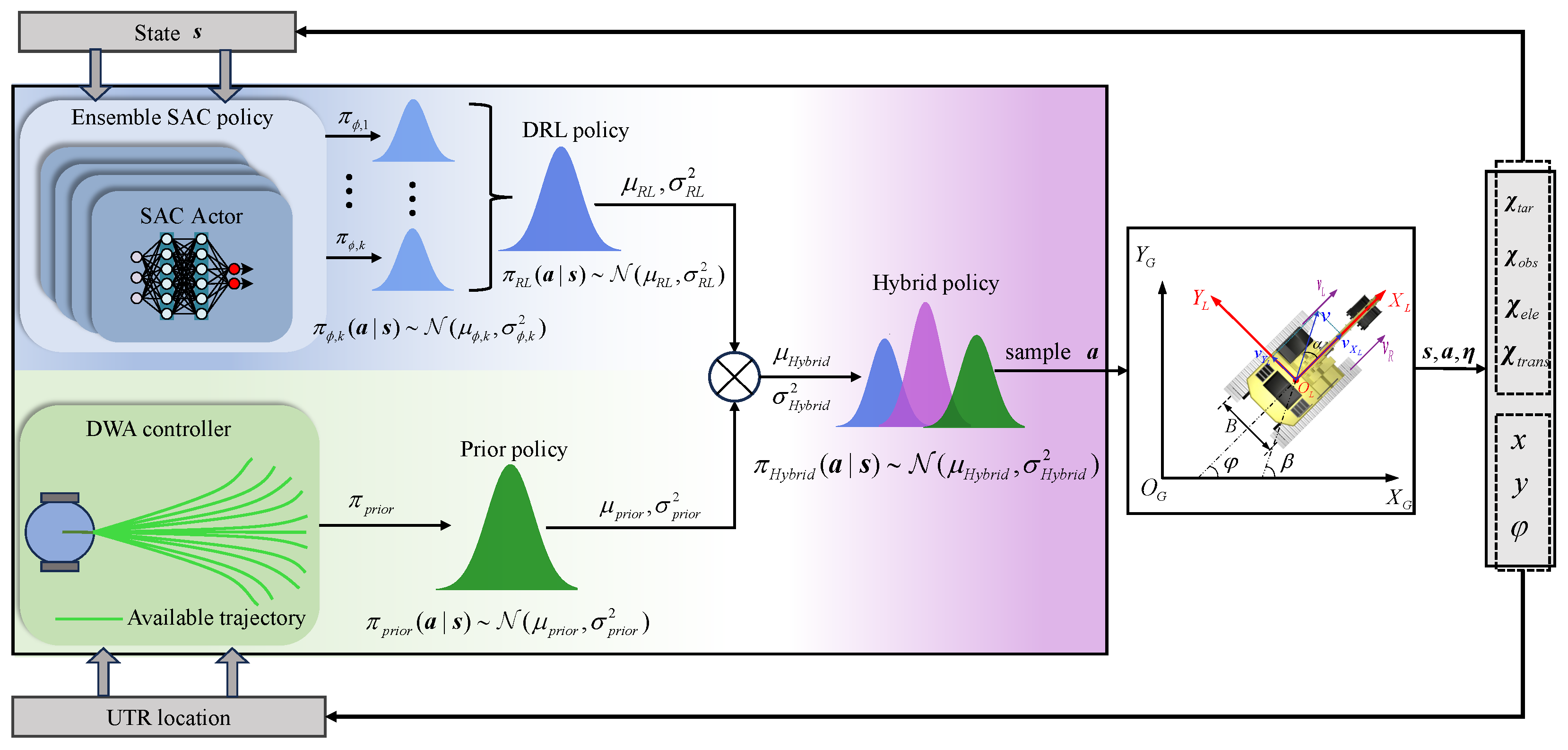
4. SAC-Based Hybrid Policy

In this section, we provide a detailed explanation of the implementation details of the proposed SAC-based Hybrid Policy (SAC-HP) algorithm.

Although the standard SAC algorithm [24] demonstrates outstanding performance in navigation tasks, its performance is limited by the following reasons. Firstly, when the dimensions of the state and action spaces are high, the agent requires significant exploration time at the beginning to collect sufficient experience. Secondly, due to the black box nature of deep networks, DRL policies might overfit the training environment, reducing the safety and adaptability in new environments.

The SAC-HP framework is illustrated in Figure 5. SAC-HP consists of two primary components: the DRL policy and the classical (prior) policy. The robot’s actions are determined jointly by these two policies and can be expressed using the following equation:

$${\pi }_{hybrid}\left(\mathit{a}\mid \mathit{s}\right)={\displaystyle \frac{1}{\mathbb{Z}}}\left({\pi }_{RL}\left(\mathit{a}\mid \mathit{s}\right)•{\pi }_{prior}\left(\mathit{a}\mid \mathit{s}\right)\right),$$

(26)

where ${\pi }_{RL}\left(\mathit{a}\mid \mathit{s}\right)$ represents the DRL policy, and ${\pi }_{prior}\left(\mathit{a}\mid \mathit{s}\right)$ denotes the prior policy derived from classical controllers (i.e., DWA). $\mathbb{Z}$ is a normalization factor. Specifically, $\mathbb{Z}$ ensures that the resulting hybrid policy distribution remains a valid probability distribution after the multiplicative fusion of the learned DRL policy ${\pi }_{RL}\left(\mathit{a}\mid \mathit{s}\right)$ and the prior controller distribution ${\pi }_{prior}\left(\mathit{a}\mid \mathit{s}\right)$. When both components are Gaussian distributions, their product results in an unnormalized Gaussian, and $\mathbb{Z}$ corresponds to the integral of this product over the action space. In practice, the parameters of the fused distribution (mean and variance) can be derived in closed form using Gaussian product rules (i.e., Equation (31)), and the normalization constant is implicitly handled within this derivation.

In the SAC algorithm, the output actions from the Actor network obey an independent Gaussian distribution, ${\pi }_{\varphi }(\mathit{a}\mid \mathit{s})\sim \mathcal{N}({\mu }_{\varphi },{\sigma }_{\varphi }^2)$, where ${\mu }_{\varphi }$ represents the mean of the output actions, and ${\sigma }_{\varphi }^2$ denotes the variance of the output actions. To leverage the advantage of stochastic policies and reduce variance, we utilize ensemble learning-based uncertainty estimation techniques [26]. The ensemble consists of K agents to construct an approximately uniform and robust mixture model. The predicted outputs of the ensemble are fuses to a single Gaussian distribution with a mean ${\mu }_{RL}$ and variance ${\sigma }_{RL}^2$, which is written as

$${\mu }_{\mathrm{RL}}(\mathit{s})=K^{-1}\sum _{k=1}^K{\mu }_{{\pi }_{\varphi ,k}}(\mathit{s}),$$

(27)

$${\sigma }_{\mathrm{RL}}^2(\mathit{s})=K^{-1}\sum _{k=1}^K({\sigma }_{{\pi }_{\varphi ,k}}^2(\mathit{s})+{\mu }_{{\pi }_{\varphi ,k}}^2(\mathit{s}))-{\mu }_{\mathrm{RL}}^2(\mathit{s}),$$

(28)

where ${\mu }_{{\pi }_{\varphi ,k}}$ and ${\sigma }_{{\pi }_{\varphi ,k}}^2$ represent the mean and variance of the individual DRL policy ${\pi }_{\varphi }\left(\mathit{a}\mid \mathit{s}\right)$, respectively.

Once the DWA controller predicts the optimal linear velocity $v_{DWA}$ and angular velocity ${\omega }_{DWA}$, the optimal angular velocities of the left and right driving wheels can be calculated based on Equations (1) and (3) as

$$\left\{\begin{array}{c}{\omega }_L^{prior}={\displaystyle \frac{2{\nu }_{DWA}+{\omega }_{DWA}B}{2r(1-{\zeta }_L)}}\hfill \\ {\omega }_R^{prior}={\displaystyle \frac{2{\nu }_{DWA}-{\omega }_{DWA}B}{2r(1-{\zeta }_R)}}\hfill \end{array}\right..$$

(29)

Furthermore, the preliminary action $a_{prior}=[{\omega }_L^{prior},{\omega }_R^{prior}]$ output from the DWA controller can be obtained. To acquire a distributional action from a prior controller, assuming the variance of the prior policy is ${\sigma }_{\mathrm{prior}}^2=0.3$, with a mean ${\mu }_{prior}$ corresponding to the prior controller’s deterministic output ${\mu }_{prior}=a_{prior}$. Thus, the prior policy can be expressed as ${\pi }_{prior}\left(\mathit{a}\mid \mathit{s}\right)\sim \mathcal{N}\left({\mu }_{prior},{\sigma }_{prior}^2\right)$. The prior policy ${\pi }_{prior}\left(\mathit{a}\mid \mathit{s}\right)$ is able to guide the agent within a certain range of area at the beginning, thereby avoiding unnecessary high-risk exploratory actions.

Furthermore, Equation (26) can be rewritten as

$${\pi }_{hybrid}\left(\mathit{a}\mid \mathit{s}\right)\sim \mathcal{N}\left({\mu }_{hybrid},{\sigma }_{hybrid}^2\right),$$

(30)

$${\mu }_{hybrid}={\displaystyle \frac{{\mu }_{\mathrm{RL}}{\sigma }_{prior}^2+{\mu }_{prior}{\sigma }_{\Pi }^2}{{\sigma }_{\mathrm{RL}}^2+{\sigma }_{prior}^2}},{\sigma }_{RL}^2={\displaystyle \frac{{\sigma }_{prior}^2{\sigma }_{\mathrm{RL}}^2}{{\sigma }_{prior}^2+{\sigma }_{\mathrm{RL}}^2}},$$

(31)

The details of the hybrid policy are described in Algorithm 1.

Algorithm 1 SAC-based Hybrid Policy

Require: Initialize ensemble of K SAC policies $\{{\pi }_1,{\pi }_2,\dots ,{\pi }_K\}$; prior variance ${\sigma }_{\mathrm{prior}}^2=0.3$; Initialize experience replay buffer $\mathcal{D}$; Set update frequency $f_c$ and max iteration $I_m$. 1: for$i=1$ to $I_m$ do 2:     Randomly select one agent from the ensemble 3:     for $k=1$ to K do 4:         Get current state ${\mathit{s}}_t$ 5:         Sample action from k-th SAC agent: ${\mathit{a}}_k\sim {\pi }_k(·\mid {\mathit{s}}_t)$ 6:         Compute mean ${\mu }_k$ and variance ${\sigma }_k^2$ of action distribution 7:     end for 8:     Compute SAC ensemble Gaussian: $${\mu }_{RL}={\displaystyle \frac{1}{K}}\sum _{k=1}^K{\mu }_k,{\sigma }_{RL}^2={\displaystyle \frac{1}{K}}\sum _{k=1}^K({\sigma }_k^2+{\mu }_k^2)-{\mu }_{RL}^2$$ 9:     Predict DWA prior action ${\mathit{a}}_{\mathrm{prior}}=[{\omega }_L,{\omega }_R]$ 10:     Set prior distribution: ${\mu }_{\mathrm{prior}}={\mathit{a}}_{\mathrm{prior}},{\sigma }_{\mathrm{prior}}^2=0.3$ 11:     Compute hybrid Gaussian policy: $${\mu }_{\mathrm{hybrid}}={\displaystyle \frac{{\mu }_{RL}{\sigma }_{\mathrm{prior}}^2+{\mu }_{\mathrm{prior}}{\sigma }_{RL}^2}{{\sigma }_{RL}^2+{\sigma }_{\mathrm{prior}}^2}},{\sigma }_{\mathrm{hybrid}}^2={\displaystyle \frac{{\sigma }_{RL}^2{\sigma }_{\mathrm{prior}}^2}{{\sigma }_{RL}^2+{\sigma }_{\mathrm{prior}}^2}}$$ 12:     Sample action ${\mathit{a}}_t\sim \mathcal{N}({\mu }_{\mathrm{hybrid}},{\sigma }_{\mathrm{hybrid}}^2)$ 13:     Execute ${\mathit{a}}_t$ and observe $({\mathit{s}}_{t+1},r,d)$ 14:     Store transition $({\mathit{s}}_t,{\mathit{a}}_t,r,{\mathit{s}}_{t+1},d)$ in buffer $\mathcal{D}$ 15:     if $d==\mathrm{True}$ then 16:         Reset environment 17:     end if 18:     if $imod{f}_c==0$ then 19:         Update all K SAC agents by minimizing Equations (6) and (8) 20:     end if 21: end for Ensure: Optimal policy ${\pi }_{\mathrm{hybrid}}^{*}$

In the SAC-HP framework, each iteration begins by sampling actions from an ensemble of K SAC policies. These K outputs are first aggregated to form a robust and approximately uniform Gaussian distribution ${\pi }_{RL}\left(\mathit{a}\mid \mathit{s}\right)$ (i.e., Equations (27) and (28)), which captures policy uncertainty and reduces overfitting. In parallel, the DWA controller produces a deterministic action based on the current robot state, which is modeled as a fixed-variance Gaussian distribution ${\pi }_{prior}\left(\mathit{a}\mid \mathit{s}\right)$. These two distributions are then fused into a hybrid Gaussian policy ${\pi }_{hybrid}\left(\mathit{a}\mid \mathit{s}\right)$ using Equation (31). An action is sampled from ${\pi }_{hybrid}\left(\mathit{a}\mid \mathit{s}\right)$, executed in the environment, and the resulting transition is stored in the replay buffer. All ensemble SAC agents are updated based on the collected experience. This hierarchical fusion structure ensures both safe exploration and generalizable policy learning under rugged terrain conditions. Note that the hybrid action is sampled at every decision-making step during both training and evaluation. This ensures that the prior (DWA) continuously guides the exploration throughout training and contributes to policy robustness during testing.

5. Simulation Results

Compared against baselines, several experiments were designed to verify the performance of the proposed hybrid policy controller for navigation.

5.1. Simulation Environment Setting

The simulation area (i.e., $50\mathrm{m}\times 50\mathrm{m}$) with unstructured obstacles was configured as shown in Figure 6. Purple cylindrical shapes represent discrete binary obstacles, while the contour regions indicate continuous rugged terrains. Assuming that the UTV will encounter random slipping disturbances within the rugged terrain areas, the task objective is to enable the UTV to navigate from the blue starting point to the red endpoint. The experimental configuration parameters and SAC training hyperparameters are listed in

Table 2. Parametric setting in the simulation.

Parameter	Description	Value
B	Track gauge	1 m
r	Radius of the track drive sprocket	0.5 m
${\omega }_{max}$	Maximum angular velocities of the left and right track drive sprockets	1.5 rad/s
${\epsilon }_{col}$; ${\epsilon }_{safe}$	Boundary of collision; boundary of safe	0.5 m; 0.5 m
$d_{goal}$; $d_{near}$	Boundary of goal; goal boundary threshold for positive reward	1 m; 10 m
$d_{max}$	Maximum scanning range of sensor	15 m
N	Number of separated intervals within the sensor reading	10
M; N	Elevation grid range; elevation grid size	10 m; 20
$\tau$	Number of samples used for linear velocity averaging	20

and

Table 3. Training configuration.

Parameter	Value
Maximum steps per episode	1000
Maximum training steps	$2.5\times {10}^5$
Discount factor	0.99
Initial temperature coefficient	0.12
Learning rate	$3\times {10}^{-4}$
Hidden units	512
Batch size	256
$(w_1\sim w_6)$	$(2,1.5,20,10,10,1)$

, respectively. Notably, the maximum rotational speed of the UTV’s left and right drive wheels is $1.5\mathrm{rad}/\mathrm{s}$.

The control time step was set to 0.2 s throughout training and evaluation. This choice was motivated by three considerations: (1) The dynamic response delay of tracked vehicles is typically around 0.15–0.2 s, making finer control updates less impactful [1]. (2) The onboard sensor suite, including LiDAR, operates at a sampling frequency of 5 Hz, corresponding to one observation every 0.2 s. (3) Empirical tests indicate that this step size provides a good tradeoff between control accuracy and computational efficiency, especially in long-horizon navigation scenarios. This setting ensures stable policy learning without excessive computational overhead.

5.2. Performance of the Extended State Space

To evaluate the impact of the extended state space on the navigation performance of UTV, we trained four separate agents. The state space and training environment configurations for these agents are detailed in

Table 4. Configuration of agents and environment.

Agent Name	State Space	Environment Setting
Agent 1 1	$\mathit{S}=\left[\begin{array}{c}{\mathit{\chi }}_{tar},{\mathit{\chi }}_{obs}\end{array}\right]$	Without track slipping
Agent 2 2	$\mathit{S}=\left[\begin{array}{c}{\mathit{\chi }}_{tar},{\mathit{\chi }}_{obs},{\mathit{\chi }}_{ele}\end{array}\right]$	Without track slipping
Agent 3 3	$\mathit{S}=\left[\begin{array}{c}{\mathit{\chi }}_{tar},{\mathit{\chi }}_{obs},{\mathit{\chi }}_{ele}\end{array}\right]$	With random track slipping
Agent 4 4	$\mathit{S}=\left[\begin{array}{c}{\mathit{\chi }}_{tar},{\mathit{\chi }}_{obs},{\mathit{\chi }}_{ele},{\mathit{\chi }}_{trans}\end{array}\right]$	With random track slipping

¹ The state space includes only target position state (9) and obstacle position state (11), with no slipping disturbances introduced into the environment. ² The state space includes target position state (9), obstacle position state (11), and local elevation information (14), with no slipping disturbances introduced into the environment. ³ The state space includes target position state (9), obstacle position state (11), and local elevation information (14), with random slipping disturbances introduced into the environment. ⁴ The state space includes target position state (9), obstacle position state (11), local elevation information (14), and UTV’s attitude change (15), with random slipping disturbances introduced into the environment.

.

During training, each episode started with different initial positions and target points, enabling the agent to explore various behaviors and regions. For Agents 3 and 4, the map area within $25\mathrm{m}<y<50\mathrm{m}$ was configured as a low-friction region. When the UTV operates in this region, random slipping rates are applied to the left and right tracks. The slipping rates were uniformly sampled from the range ${\zeta }_L,{\zeta }_R\sim U\left(0,0.5\right)$.

Figure 7 highlights the performance differences among the four agents. According to the blue curve in Figure 7c, the results demonstrate that incorporating elevation information into the state space allowed the UTV to detect terrain undulations, enabling it to avoid deep pits and steep slopes while navigating through relatively smooth regions toward the target (i.e., Agent 2). In contrast, the UTV failed to avoid rugged terrain and fell into a deep pit at approximately the 200th time step according to the red curve in Figure 7c.

Under slipping disturbances, the trajectory planned by Agent 3 exhibited significant oscillations and failed to reach the goal according to the yellow curve in Figure 7c. In contrast, the trajectory planned by Agent 4 was much smoother, indicating that the introduction of agent pose changes in the state space allows the UTV to effectively mitigate the effects of slip disturbances.

5.3. Reward Function Evaluation

To validate the influence of the $R_6$ in the reward function (24), we recorded the linear velocity curve over time during the driving stage. Figure 8 illustrates the velocity outputs of two agents (i.e., one trained with $R_6$ and the other without) during the driving stage. Both agents were trained using the complete state space, with random slip disturbances introduced in the environment (i.e., same as the configuration of Agent 4 described in Section 5.2). As shown in

Table 5. Results of reward function evaluation.

	Total Time Steps	Average Velocity [m/s]	Variance of Velocity [m/s]
With $R_6$ in Equation (25)	287	0.69	0.0019
Without $R_6$ in Equation (25)	483	0.42	0.0152

, when $R_6$ was included in the reward function, the UTV reached the destination at the 287th time step, with an average linear velocity of 0.69 and a variance of 0.0019 (i.e., represented by the red curve). In contrast, when $R_6$ was excluded, the UTV took 483 time steps to reach the destination, with an average linear velocity of 0.42 and a variance of 0.0152 (i.e., represented by the blue curve). The experimental results indicate that the energy optimization term in the reward function (24) significantly reduces velocity oscillations in the UTV, enabling it to operate more smoothly and at higher speeds.

5.4. Performance of SAC-HP

The SAC algorithm based on the extended state space enables the robot to handle continuous rugged terrain and slip disturbances, thereby improving the safety and robustness of the navigation process. However, in large-scale environments (i.e., long-sequence navigation environments) with extensive map coverage, it becomes difficult for the robot to reach the target with a larger exploration space. Additionally, deep reinforcement learning generally suffers from poor generalization performance. When the robot enters an unknown environment, it is challenging to plan a collision-free path to the target using the overfitted model obtained from the previous experience.

To address the issue of slow exploration and difficulty in reaching the target point in long-sequence environments, the SAC-based Hybrid Policy (SAC-HP) algorithm is proposed.

We trained the agent in a long-sequence environment of 60 m by 100 m. The robot was able to avoid obstacles and navigate to the target with the trained model.

As shown in Figure 9, the cumulative reward value obtained by the agent in each episode is plotted as the number of algorithm iterations increases. Compared to the classic SAC algorithm, the blue curve in Figure 9 represents that the SAC-HP algorithm, with the reward curve converging at approximately 3400, has a 16% improvement compared to SAC, showing a significantly faster convergence rate. This indicates that the learning efficiency in long-sequence environments is enhanced by introducing DWA as a prior policy to guide the agent’s early exploration.

To validate the generalization performance of the model, we conducted tests in a random environment. As shown in Figure 10, the robot’s navigation trajectory in scenarios with random obstacles and terrains is plotted. The experimental results demonstrate that, in the random environment, the robot was able to successfully reach the target and avoid obstacles and rugged terrain.

5.5. Comparison Between Baselines

To evaluate the superiority of the proposed SAC-HP algorithm, five baselines were selected for comparison experiments (i.e., SAC [24], Twin Delayed Deep Deterministic Policy Gradient (TD3) [27], Proximal Policy Optimization (PPO) [28], APF [29], and DWA [30]). The experiments were conducted in two scenarios: one was with slipping disturbance (i.e., Env.a), and the other one was without slipping disturbance (i.e., Env.b), using a randomly generated 50 × 100 map. Each experiment was repeated for 500 episodes.

We established four metrics to evaluate the performance of various algorithms, including Average Path Length (APL), Average Time Steps (ATS), Elevation Standard Deviation (ESD), and Success Rates (SR):

• APL (Average Path Length): APL represents the mean total length of the path traveled by the robot from the starting point to the target point across all successful experimental episodes. It is used to assess the efficiency of path planning algorithms:

  $$L_{\mathrm{avg}}={\displaystyle \frac{1}{N_{ep}}}\sum _{i=1}^{N_{ep}}{L}_i,$$

  (32)

  where $L_i$ is the total path length in the i-th successful episode, and $N_{ep}$ is the total number of successful episodes.
• ATS (Average Time Steps): ATS reflects the mean number of time steps required for the robot to complete the navigation task, measuring the temporal efficiency of the algorithm:

  $$T_{\mathrm{avg}}={\displaystyle \frac{1}{N_{ep}}}\sum _{i=1}^{N_{ep}}{T}_i,$$

  (33)

  where $T_i$ is the total number of time steps in the i-th successful episode.
• ESD (Elevation Standard Deviation): The elevation standard deviation for each episode represents the variation in the robot’s height along the navigation path during that episode. It is used to assess the smoothness of the planned trajectory and the robot’s adaptability to complex terrains:

  $${\sigma }_h=\sqrt{{\displaystyle \frac{1}{t_{ep}}}\sum _{j=1}^{t_{ep}}{(h_j-\overline{h})}^2},$$

  (34)

  where $h_j$ is the height of the j-th point on the path, $\overline{h}$ is the mean height, and $t_{ep}$ is the total number of path points. Next, calculate the average of all episodes:

  $${\mu }_{{\sigma }_h}={\displaystyle \frac{1}{N_{ep}}}\sum _{i=1}^{N_{ep}}{\sigma }_h^{(i)},$$

  (35)

  where $N_{ep}$ is the total number of episodes.
• SR (Success Rates): SR quantifies the proportion of episodes in which the robot successfully reached the target point, providing a measure of the algorithm’s reliability and robustness

  $$\mathrm{SR}={\displaystyle \frac{N_{success}}{N_{ep}}}\times 100\%,$$

  (36)

  where $N_{success}$ is the number of successful episodes.

As shown in

Table 6. Performance comparison of SAC-HP and baseline algorithms across metrics.

	Env.a 1				Env.b 2
Algorithm	APL (m)	ATS	ESD (m)	SR (%)	APL (m)	ATS	ESD (m)	SR (%)
SAC-HP	96.353	851	0.113	92	96.812	993	0.239	91
SAC	98.281	891	0.175	86	98.921	1041	0.287	80
TD3	99.729	896	0.291	83	100.395	1049	0.451	76
PPO	102.613	1016	0.301	79	104.832	1153	0.557	71
DWA	99.251	997	2.214	91	115.632	1732	2.269	44
APF	100.337	1005	2.103	88	120.527	1885	2.255	39

¹ Env.a: Without slipping disturbance. ² Env.b: With slipping disturbance.

, in the cases without slipping disturbances (i.e., Env.a), it can be observed that SAC-HP outperformed traditional DRL algorithms, achieving a success rate improvement of over 6%. Moreover, compared to SAC, it has a 1.9% improvement on APL, 4.5% improvement on ATS, and 35% improvement on ESD. In the cases with slipping disturbances (i.e., Env.b), the performance of the DRL baseline model dropped sharply, while the success rate of SAC-HP was able to maintain over 90%. The results demonstrate its robustness and reliability in completing navigation tasks, even in challenging environments.

In the cases without slipping disturbances, APF and DWA exhibited higher success rates than some DRL algorithms. However, when slipping disturbances are introduced, the performance of traditional local planning algorithms deteriorates significantly. This indicates that DRL-based algorithms, particularly SAC-HP, have a stronger capability to cope with random disturbances. Furthermore, traditional planning algorithms struggle to handle rugged terrains, as evidenced by their significantly higher elevation standard deviations in each experimental episode compared to DRL algorithms. This confirms the advantage of DRL algorithms in generating smoother trajectories and maintaining stability under complex terrain conditions.

6. Conclusions

This paper presents a novel approach for real-time autonomous path planning of UTVs in unknown off-road environments, utilizing the SAC-based Hybrid Policy (SAC-HP) algorithm. By integrating the kinematic analysis of tracked vehicles, a new state space and action space are designed to account for rugged terrain features and the interaction between the tracks and the ground. This enables the UTV to implicitly learn policies for safely traversing rugged terrains while minimizing the effects of slipping disturbances.

The proposed SAC-HP algorithm combines the advantages of deep reinforcement learning (DRL) with prior control policies (i.e., Dynamic Window Approach) to enhance exploration efficiency and generalization performance in long-sequence environments. Experimental results show that SAC-HP converged 16% faster than the traditional SAC algorithm and achieved a more than 6% higher success rate in rough terrain scenarios. Additionally, it reduced the elevation standard deviation by 35% (from 0.175 m to 0.113 m), indicating smoother trajectories, and decreased the average time steps by 4.5%. The introduction of the energy optimization term in the reward function also effectively reduced velocity oscillations, allowing the robot to operate more smoothly and at higher speeds.

Tests conducted in random environments with obstacles and rugged terrain demonstrate the robustness of the model, as the robot was able to autonomously avoid obstacles and navigate to the target location, even in unknown environments. These results highlight the potential of the SAC-HP algorithm to enhance the safety, robustness, and efficiency of UTV in complex environments.

Although the SAC-HP algorithm demonstrates strong performance in autonomous navigation for UTVs, several potential improvements can be explored in future work. First, incorporating additional environmental factors, such as water currents and dynamic obstacles, could enhance the algorithm’s adaptability to complex off-road environments. Secondly, the scalability of the algorithm for larger and more complex terrains, particularly in high-dimensional state and action spaces, warrants further investigation. Moreover, although the SAC-HP agent significantly reduces training time compared to vanilla SAC, achieving satisfactory performance within extremely low iteration counts remains a challenge. To address this, future work could explore few-shot reinforcement learning [31] or RL with expert demonstrations [32] to enable rapid policy adaptation in resource-constrained or time-critical deployment scenarios.

In addition, real-world deployment remains a major challenge for DRL-based methods. Potential remedies such as domain randomization [33], noise injection during training [34], and human-guided RL [35] may help close the simulation-to-reality gap. Moreover, robust sensor fusion using IMU, LiDAR, and visual input can enhance policy generalization under uncertain terrain conditions [36,37]. Future extensions of SAC-HP will integrate these mechanisms to facilitate more reliable and scalable deployment in the field.

Future work could also explore extending the SAC-HP framework to aerial systems, such as fixed-wing UAVs. For example, the ensemble-based policy fusion used in our UTV strategy could be adapted to address UAV-specific constraints (e.g., roll angle limits and aerodynamic load factors). Insights from UAV trajectory optimization studies [38] could inform such extensions, bridging the gap between ground and aerial autonomous navigation.

References

1. Amokrane, S.B.; Laidouni, M.Z.; Adli, T.; Madonski, R.; Stanković, M. Active disturbance rejection control for unmanned tracked vehicles in leader–follower scenarios: Discrete-time implementation and field test validation. Mechatronics 2024, 97, 103114. [Google Scholar] [CrossRef]
2. Ugenti, A.; Galati, R.; Mantriota, G.; Reina, G. Analysis of an all-terrain tracked robot with innovative suspension system. Mech. Mach. Theory 2023, 182, 105237. [Google Scholar] [CrossRef]
3. Zou, T.; Angeles, J.; Hassani, F. Dynamic modeling and trajectory tracking control of unmanned tracked vehicles. Robot. Auton. Syst. 2018, 110, 102–111. [Google Scholar] [CrossRef]
4. Zhai, L.; Liu, C.; Zhang, X.; Wang, C. Local Trajectory Planning for Obstacle Avoidance of Unmanned Tracked Vehicles Based on Artificial Potential Field Method. IEEE Access 2024, 12, 19665–19681. [Google Scholar] [CrossRef]
5. Aradi, S. Survey of Deep Reinforcement Learning for Motion Planning of Autonomous Vehicles. IEEE Trans. Intell. Transp. Syst. 2022, 23, 740–759. [Google Scholar] [CrossRef]
6. Zhang, Y.; Zhao, W.; Wang, J.; Yuan, Y. Recent progress, challenges and future prospects of applied deep reinforcement learning: A practical perspective in path planning. Neurocomputing 2024, 608, 128423. [Google Scholar] [CrossRef]
7. Gök, M. Dynamic path planning via Dueling Double Deep Q-Network (D3QN) with prioritized experience replay. Appl. Soft Comput. 2024, 158, 111503. [Google Scholar] [CrossRef]
8. Maoudj, A.; Hentout, A. Optimal path planning approach based on Q-learning algorithm for mobile robots. Appl. Soft Comput. 2020, 97, 106796. [Google Scholar] [CrossRef]
9. Zhou, W.; Zhang, C.; Chen, S. Dual deep Q-learning network guiding a multiagent path planning approach for virtual fire emergency scenarios. Appl. Intell. 2023, 53, 21858–21874. [Google Scholar] [CrossRef]
10. Rao, Z.; Wu, Y.; Yang, Z.; Zhang, W.; Lu, S.; Lu, W.; Zha, Z. Visual Navigation With Multiple Goals Based on Deep Reinforcement Learning. IEEE Trans. Neural Networks Learn. Syst. 2021, 32, 5445–5455. [Google Scholar] [CrossRef]
11. Guo, H.; Ren, Z.; Lai, J.; Wu, Z.; Xie, S. Optimal navigation for AGVs: A soft actor–critic-based reinforcement learning approach with composite auxiliary rewards. Eng. Appl. Artif. Intell. 2023, 124, 106613. [Google Scholar] [CrossRef]
12. Li, C.; Yue, X.; Liu, Z.; Ma, G.; Zhang, H.; Zhou, Y.; Zhu, J. A modified dueling DQN algorithm for robot path planning incorporating priority experience replay and artificial potential fields. Appl. Intell. 2025, 55, 366. [Google Scholar] [CrossRef]
13. Zhang, Y.; Li, C. On Hierarchical Path Planning Based on Deep Reinforcement Learning in Off- Road Environments. In Proceedings of the 2024 10th International Conference on Automation, Robotics and Applications (ICARA), Athens, Greece, 22–24 February 2024; pp. 461–465. [Google Scholar] [CrossRef]
14. Tang, C.; Peng, T.; Xie, X.; Peng, J. 3D path planning of unmanned ground vehicles based on improved DDQN. J. Supercomput. 2025, 81, 276. [Google Scholar] [CrossRef]
15. Zhang, K.; Niroui, F.; Ficocelli, M.; Nejat, G. Robot Navigation of Environments with Unknown Rough Terrain Using deep Reinforcement Learning. In Proceedings of the 2018 IEEE International Symposium on Safety, Security, and Rescue Robotics (SSRR), Philadelphia, PA, USA, 6–8 August 2018; pp. 1–7. [Google Scholar] [CrossRef]
16. Weerakoon, K.; Sathyamoorthy, A.J.; Patel, U.; Manocha, D. TERP: Reliable Planning in Uneven Outdoor Environments using Deep Reinforcement Learning. In Proceedings of the 2022 International Conference on Robotics and Automation (ICRA), Philadelphia, PA, USA, 23–27 May 2022; pp. 9447–9453. [Google Scholar] [CrossRef]
17. Nguyen, A.; Nguyen, N.; Tran, K.; Tjiputra, E.; Tran, Q.D. Autonomous Navigation in Complex Environments with Deep Multimodal Fusion Network. In Proceedings of the 2020 IEEE/RSJ International Conference on Intelligent Robots and Systems (IROS), Las Vegas, NV, USA, 24 October 2020–24 January 2021; pp. 5824–5830. [Google Scholar] [CrossRef]
18. Viadero-Monasterio, F.; Meléndez-Useros, M.; Zhang, H.; Boada, B.L.; Boada, M.J.L. Signalized Traffic Management Optimizing Energy Efficiency Under Driver Preferences for Vehicles With Heterogeneous Powertrains. IEEE Trans. Consum. Electron. 2025. [Google Scholar] [CrossRef]
19. Rana, K.; Dasagi, V.; Haviland, J.; Talbot, B.; Milford, M.; Sünderhauf, N. Bayesian controller fusion: Leveraging control priors in deep reinforcement learning for robotics. Int. J. Robot. Res. 2023, 42, 123–146. [Google Scholar] [CrossRef]
20. Wu, J.; Huang, Z.; Hu, Z.; Lv, C. Toward Human-in-the-Loop AI: Enhancing Deep Reinforcement Learning via Real-Time Human Guidance for Autonomous Driving. Engineering 2023, 21, 75–91. [Google Scholar] [CrossRef]
21. Cheng, R.; Verma, A.; Orosz, G.; Chaudhuri, S.; Yue, Y.; Burdick, J. Control regularization for reduced variance reinforcement learning. In Proceedings of the International Conference on Machine Learning, Long Beach, CA, USA, 9–15 June 2019; pp. 1141–1150. [Google Scholar]
22. Johannink, T.; Bahl, S.; Nair, A.; Luo, J.; Kumar, A.; Loskyll, M.; Ojea, J.A.; Solowjow, E.; Levine, S. Residual Reinforcement Learning for Robot Control. In Proceedings of the 2019 International Conference on Robotics and Automation (ICRA), Montreal, QC, Canada, 20–24 May 2019; pp. 6023–6029. [Google Scholar] [CrossRef]
23. Sabiha, A.D.; Kamel, M.A.; Said, E.; Hussein, W.M. ROS-based trajectory tracking control for autonomous tracked vehicle using optimized backstepping and sliding mode control. Robot. Auton. Syst. 2022, 152, 104058. [Google Scholar] [CrossRef]
24. Haarnoja, T.; Zhou, A.; Abbeel, P.; Levine, S. Soft actor-critic: Off-policy maximum entropy deep reinforcement learning with a stochastic actor. In Proceedings of the International Conference on Machine Learning, Stockholm, Sweden, 10–15 July 2018; pp. 1861–1870. [Google Scholar]
25. Shi, H.; Shi, L.; Xu, M.; Hwang, K.S. End-to-End Navigation Strategy With Deep Reinforcement Learning for Mobile Robots. IEEE Trans. Ind. Inform. 2020, 16, 2393–2402. [Google Scholar] [CrossRef]
26. Lakshminarayanan, B.; Pritzel, A.; Blundell, C. Simple and scalable predictive uncertainty estimation using deep ensembles. In Advances in Neural Information Processing Systems; MIT Press: Cambridge, MA, USA, 2017; Volume 30. [Google Scholar]
27. Fujimoto, S.; van Hoof, H.; Meger, D. Addressing Function Approximation Error in Actor-Critic Methods. In Proceedings of the 35th International Conference on Machine Learning, Stockholm, Sweden, 10–15 July 2018; Proceedings of Machine Learning Research Volume 80. pp. 1587–1596. [Google Scholar]
28. Schulman, J.; Wolski, F.; Dhariwal, P.; Radford, A.; Klimov, O. Proximal policy optimization algorithms. arXiv 2017, arXiv:1707.06347. [Google Scholar]
29. Yang, H.; He, Y.; Xu, Y.; Zhao, H. Collision Avoidance for Autonomous Vehicles Based on MPC With Adaptive APF. IEEE Trans. Intell. Veh. 2024, 9, 1559–1570. [Google Scholar] [CrossRef]
30. Yang, H.; Xu, X.; Hong, J. Automatic Parking Path Planning of Tracked Vehicle Based on Improved A* and DWA Algorithms. IEEE Trans. Transp. Electrif. 2023, 9, 283–292. [Google Scholar] [CrossRef]
31. Wang, Z.; Fu, Q.; Chen, J.; Wang, Y.; Lu, Y.; Wu, H. Reinforcement learning in few-shot scenarios: A survey. J. Grid Comput. 2023, 21, 30. [Google Scholar] [CrossRef]
32. Elallid, B.B.; Benamar, N.; Bagaa, M.; Kelouwani, S.; Mrani, N. Improving Reinforcement Learning with Expert Demonstrations and Vision Transformers for Autonomous Vehicle Control. World Electr. Veh. J. 2024, 15, 585. [Google Scholar] [CrossRef]
33. Garcia, R.; Strudel, R.; Chen, S.; Arlaud, E.; Laptev, I.; Schmid, C. Robust Visual Sim-to-Real Transfer for Robotic Manipulation. In Proceedings of the 2023 IEEE/RSJ International Conference on Intelligent Robots and Systems (IROS), Detroit, MI, USA, 1–5 October 2023; pp. 992–999. [Google Scholar] [CrossRef]
34. Joshi, B.; Kapur, D.; Kandath, H. Sim-to-Real Deep Reinforcement Learning Based Obstacle Avoidance for UAVs Under Measurement Uncertainty. In Proceedings of the 2024 10th International Conference on Automation, Robotics and Applications (ICARA), Athens, Greece, 22–24 February 2024; pp. 278–284. [Google Scholar] [CrossRef]
35. Wu, J.; Zhou, Y.; Yang, H.; Huang, Z.; Lv, C. Human-Guided Reinforcement Learning With Sim-to-Real Transfer for Autonomous Navigation. IEEE Trans. Pattern Anal. Mach. Intell. 2023, 45, 14745–14759. [Google Scholar] [CrossRef] [PubMed]
36. Ou, Y.; Cai, Y.; Sun, Y.; Qin, T. Autonomous Navigation by Mobile Robot with Sensor Fusion Based on Deep Reinforcement Learning. Sensors 2024, 24, 3895. [Google Scholar] [CrossRef]
37. Tan, J. A Method to Plan the Path of a Robot Utilizing Deep Reinforcement Learning and Multi-Sensory Information Fusion. Appl. Artif. Intell. 2023, 37, 2224996. [Google Scholar] [CrossRef]
38. Machmudah, A.; Shanmugavel, M.; Parman, S.; Manan, T.S.A.; Dutykh, D.; Beddu, S.; Rajabi, A. Flight Trajectories Optimization of Fixed-Wing UAV by Bank-Turn Mechanism. Drones 2022, 6, 69. [Google Scholar] [CrossRef]
Figure 1. Kinematic model of UTV.
Wevj 16 00359 g001
Figure 2. SAC framework.
Wevj 16 00359 g002
Figure 3. Local elevation information.
Wevj 16 00359 g003
Figure 4. Illustration of a UTV navigation in an environment with obstacles.
Wevj 16 00359 g004
Figure 5. The SAC-HP framework. The hybrid policy π h y b r i d generates the hybrid action a directly via a combination of the DRL policy π R L based on SAC and the classical (prior) policy π p r i o r based on DWA controller. The DRL policy is obtained by using an ensemble SAC policy that is a mixture of a single SAC policy π ϕ , k a s with state s as an input, which is defined in Section 3.1. The DWA controller uses the UTV’s position as inputs.
Wevj 16 00359 g005
Figure 6. Experimental scenario.
Wevj 16 00359 g006
Figure 7. Performance of extend state space. (a) The planned trajectories of the agents. (b) The temporal variation in the distance between the UTV and the target point. (c) The elevation values of the UTV’s position at each time step.
Wevj 16 00359 g007
Figure 8. The linear velocity curve along with time.
Wevj 16 00359 g008
Figure 9. Average reward curves.
Wevj 16 00359 g009
Figure 10. The optimal trajectory produced by SAC-HP controller in random environments.
Wevj 16 00359 g010