Abstract
Currently, the layout planning of power exchange facilities in urban areas is not perfect, which cannot effectively meet the power exchange demand of urban operating vehicles and restricts the operation of urban operating vehicles. The article proposes a vehicle power exchange demand-oriented power exchange station siting planning scheme to meet the rapid replenishment demand of operating vehicles in urban areas. The spatial and temporal distribution of power exchange demand is predicted by considering the operation law, driving law, and charging decision of drivers; the candidate sites of power exchange stations are determined based on the data of power exchange demand; the optimization model of the site selection of power exchange stations with the lowest loss time of vehicle power exchange and the lowest cost of the planning and construction of power exchange stations is established and solved by using the joint algorithm of MLP-NSGA-II; and the optimization model is compared with the traditional genetic algorithm (GA) and the Density Peak. The results show that the MLP-NSGA-II joint algorithm has the lowest cost of optimizing the location of switching stations. The results show that the MLP-NSGA-II algorithm improves the convergence efficiency by about 30.23%, and the service coverage of the optimal solution reaches 94.30%; the service utilization rate is 85.35%, which is 6.25% and 19.69% higher than that of the GA and DPC, respectively. The research content of the article can provide a design basis for the future configuration of the number and location of power exchange stations in urban areas.
1. Introduction
The battery swapping model, characterized by fast energy replenishment and strong controllability of battery management, is particularly suitable for time-sensitive commercial vehicles such as taxis and ride-hailing fleets [1]. Driven by both policy incentives and market demand, its adoption in urban transport continues to grow [2]. However, the development of supporting infrastructure lags behind, with issues such as the scattered spatial distribution and inefficient resource allocation of swap stations. These limitations lead to prolonged charging wait times and reduced operational efficiency. Therefore, scientifically planning the spatial layout of swap stations is essential to improve service coverage, optimize resource use, and enhance the coordinated development between infrastructure and urban fleet operations.
Recent studies on battery swapping have primarily focused on station-level scheduling optimization. Some works have developed models that incorporate battery health conditions and station load to enhance swap scheduling efficiency [3]. Others have explored network-level optimization by considering dynamic demand response and battery-sharing mechanisms, accounting for fluctuations in user demand and swap frequency [4]. Despite these developments, research on the spatial layout and construction planning of battery swapping infrastructure remains limited. The accurate forecasting of energy demand is a crucial prerequisite for infrastructure siting. To this end, various approaches—such as Monte Carlo simulation [5,6], trip chain theory [7,8], cumulative prospect theory [9,10], gray prediction models [11,12], LSTM neural networks [13,14], and rolling forecasting techniques [15,16]—have been employed in charging demand prediction. However, most of these models do not distinguish between charging and swapping demand. The existing studies often focus on residential charging scenarios, incorporating factors such as user charging preferences [17], urban functional zoning [18], real-time traffic flow [19], and actual charging records [20]. In contrast, there is a lack of targeted research on commercial vehicles such as taxis and ride-hailing fleets. Research on charging station siting primarily concentrates on single-objective optimization models that aim to maximize demand coverage [21,22], multi-objective models that address conflicting criteria [23,24], and capacity configuration under multi-objective constraints [25,26]. Nonetheless, few studies incorporate the unique spatiotemporal distribution of swapping demand or analyze multiple influencing factors in site planning.
In summary, there remains a significant research gap in predicting and analyzing the distinct swapping demands of commercial fleets and integrating such insights into the siting and layout of battery swapping stations. Addressing this challenge is critical to promoting the large-scale deployment of battery swapping infrastructure, particularly under the constraints of complex urban environments [27,28].
To achieve efficient matching between the battery swapping demand of urban commercial vehicles and the supply capacity of regional swapping infrastructure while balancing vehicle operational efficiency and station construction costs, this study proposes a demand-oriented hierarchical planning framework for battery swap station siting. Based on the service capacities of stations at different levels, a layout strategy is developed to determine the appropriate number and type of swap stations according to demand distribution. The proposed model is solved using an integrated MLP-NSGA-II algorithm to address the diverse energy replenishment needs within the region.
2. Analysis and Forecasting of Demand for Power Switching in Operational Vehicles
2.1. Conditions for Generating Demand for Power Switching in Operational Vehicles
The determination of whether a vehicle engenders a demand for power exchange is predicated on two conditions.
Firstly, it is necessary to ascertain whether the battery’s current remaining power SOC (state of charge) meets the demand for the subsequent trip distance. In the event that the trip distance of the next order exceeds the vehicle’s remaining range, a demand for power exchange is generated.
where is the current charge of the battery and is the maximum charge of the battery in Ah.
Secondly, the driver’s minimum SOC preference, which is defined as the value of power that the driver tends to switch when the battery power drops to a certain critical level, is a key factor in understanding the system’s behavior. In this paper, a normal distribution model is constructed to quantitatively characterize the distribution of drivers’ minimum SOC preference for switching.
where denotes the minimum SOC preference of EV users; denotes the expected value of the average minimum SOC preference, which takes the value of 0.3; and denotes the standard deviation of the minimum SOC preference, which takes the value of 0.09924.
2.2. Modeling of Demand Forecasting for Power Switching in Operational Vehicles
The main influencing factors of the demand for power exchange of operating vehicles include the operating law of operating vehicles, traveling law, and driver charging decisions. This paper extracts and analyzes the traffic trajectory dataset of operating vehicles to accurately quantify the vehicle travel process, reveal the intrinsic law of operating vehicle travel behavior, and provide a theoretical basis and empirical support for the accurate prediction of power exchange demand.
The traffic trajectory dataset records the satellite data of online taxis and cabs from 13 September to 19 September 2022 and the dataset contains the vehicle ID, trip start time, trip end time, trip start latitude and longitude, trip end latitude and longitude, and the data range is located between 117°32′ and 118°31′ east longitude and 35°55′ and 37°17′ north latitude.
2.2.1. Operating Vehicle Operating Laws Model
- (1)
- Travel distance
In this study, the trip distance of operating vehicles in urban areas was analyzed by quantitative fitting, and a statistical model was constructed with 1 km as the basic scale. The analysis results show that the trip distance data approximately obey the normal distribution after the logarithmic transformation, i.e., the raw data show the typical characteristics of the log-normal distribution, and the probability density function is expressed as follows:
where is the mileage traveled, and and are the expected value and standard deviation taken as and .
- (2)
- Departure start time distribution
Departure start time distribution refers to the operation of the vehicle in the day at all times. To start the trip time distribution law, usually in hours for the time, the departure start time distribution can be described as follows:
where denotes the number of peak hours indicates the existence of multiple travel peaks in a day, denotes the weight of the peak reflects the share of each peak in the overall travel flow, denotes the center time of the peak, and denotes the peak width of the peak. In this paper, the calibrated values of each parameter are shown in Table 1 by analyzing the operating vehicle trajectory dataset:

Table 1.
Distribution parameters of departure start time for operating vehicles.
- (3)
- Trip destinations
Through the latitude and longitude analysis of the order destination location information in the traffic dataset of operating vehicles, the typical trip destination types of operating vehicles are extracted and counted to summarize the spatial distribution characteristics of their trip destinations. The proportion of each type of destination in the overall trip is shown in Figure 1.
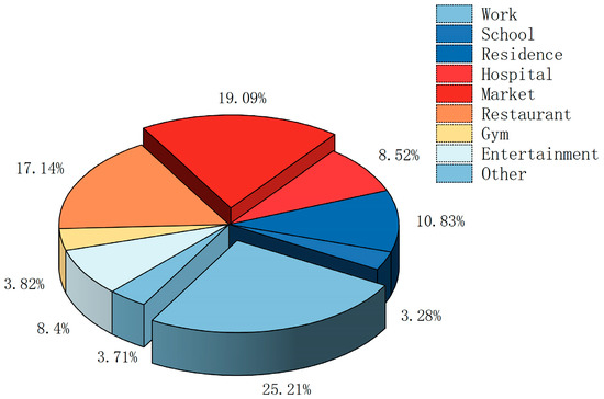
Figure 1.
Proportion of travel destinations for operating vehicles.
- (4)
- Distribution of operating order counts
The distribution of operation order times refers to the statistical distribution of the number of orders completed by each operation vehicle in the whole vehicle population in a specific time period; this paper uses the negative binomial distribution to describe the number of orders in a day of the operation vehicle, denoted as follows:
where denotes the number of vehicle operations, denotes the discrete parameter, and denotes the success probability parameter. takes the value of 3 and takes the value of 0.25 by analyzing the dataset.
2.2.2. Operating Vehicle Travel Law Model
- (1)
- Initial SOC
It has been assumed in the literature [29] that the state of charge at the moment of the vehicle’s first trip conforms to a normal distribution, and the assumption that the initial SOC of an EV is normally distributed has been verified by fitting the NHTS survey data.
where is the initial power, and and are the expected value and standard deviation taken as 0.75 and 0.1.
- (2)
- Energy consumption state
Based on the statistical analysis of the traveling speed of operating vehicles and the measured data, this study constructed a power consumption polynomial model with speed as the independent variable and determined the model parameters by data fitting [30]. The calculation formula is as follows:
where represents the formal energy consumption of the vehicle (kWh/km).
The relationship between automobile travel speed and road congestion can be expressed as follows:
where represents the actual traveling speed; represents the ideal design speed of the road (km/h); and represents the congestion level coefficient, which takes a value between 1 and 2.
According to “Urban Road Engineering Design Specification CJJ37-2012” the road grade is divided into four levels: expressway, trunk road, secondary road, and branch road [31]; for the specific design speed index of each level of road, see Table 2. In order to facilitate the calculation, this paper will be simplified with its road grade and the corresponding design speed.
Table 2.
Classification of road types and corresponding design speeds.
2.2.3. Monte Carlo Method-Based Simulation of Power Exchange Demand
This paper develops a travel behavior model for operating electric vehicles using order data. The electric vehicle energy consumption model and Amap-based road network information are integrated, and the Monte Carlo method, which has demonstrated strong performance in forecasting battery swapping demand [32,33], is employed to simulate and predict vehicle operations in urban areas. This allows for the identification of spatial and temporal patterns in swapping demand.
Assuming that the number of electric vehicles is N, the specific process is shown in Figure 2.

Figure 2.
Monte Carlo prediction of battery swapping demand forecasting process diagram.
Meanwhile, in order to simplify the model, this paper makes the following assumptions in the prediction:
- (1)
- A default vehicle owner pursues the optimal goal, i.e., the shortest distance traveled, in path selection and power exchange station selection.
- (2)
- Vehicle driving speed is only related to road type and road congestion level; i.e., under the same road type and congestion level, the vehicle driving speed is the same, independent of driver behavior.
- (3)
- Power consumption is only related to vehicle speed and road class, without taking into account factors such as air conditioning and other in-vehicle accessory equipment and weather conditions such as temperature.
3. Layout Model for the Planning of Power Exchange Stations for Operational Vehicles
3.1. Identification of Candidate Sites for Power Exchange Stations
To address the problem of optimizing the location and layout of electric vehicle power exchange stations, this study proposes to use the Monte Carlo predicted demand data for power exchange as the basis, and use the K-means clustering algorithm to cluster them to screen the candidate sites for power exchange stations.
3.2. Modeling of Switching Station Layout Planning
3.2.1. Objective Function
This paper proposes a hierarchical layout planning model for power exchange stations based on a two-layer optimization mechanism of power exchange loss time and power exchange station planning cost, and the basic assumptions of the power exchange station siting planning model are as follows:
- (1)
- The operating vehicles in the simulation area are all in the power exchange mode.
- (2)
- There are enough batteries in the power exchange station to meet the power exchange demand of the vehicles, and there is no battery waiting time.
Objective Function 1: Planning Cost of Power Exchange Station
The planning cost of the switching station is shown in Equations (9)–(12), which consists of three parts: the cost of acquiring land resources , the cost of building and constructing the switching station , and the cost of purchasing equipment .
where represents the land area of the power exchange station (m2); represents the land utilization rate of the power exchange station; represents the unit price of the land (yuan/m2); represents the unit price of the construction and building (yuan/m2); , and in the equipment procurement cost represent the number of power exchange robotic arms, power exchange batteries, and battery charging bins, respectively; and , , and are the corresponding unit prices of the equipment modules.
Objective function 2: Lost time of vehicle power exchange
Vehicle power exchange loss time mainly considers the loss time of the vehicle traveling to the power exchange station, the queuing time of the vehicle at the power exchange station, and the time of the vehicle carrying out the power exchange operation, and the objective function formula is as follows:
where represents the travel time for the vehicle to reach the switching station; represents the queuing waiting time for the vehicle at the site; represents the time for a single switching operation; and represents whether or not the vehicle is assigned to the switching station, and takes the value of 0 or 1.
3.2.2. Restrictive Condition
- (1)
- Constraints on the number of switching stations that can be built: In order to control the overall construction scale and cost, it is limited to selecting a maximum of one station to be built in the candidate location, so as to ensure the rationality and operability of resource allocation.
- (2)
- Service capacity constraints of the exchange stations: Each built exchange station has a limited service capacity and the number of vehicles it can serve shall not exceed its set maximum service capacity.
- (3)
- Maximum service radius constraints for power exchange stations: In order to safeguard the efficiency and accessibility of power exchange for vehicles, vehicles are only allowed to select power exchange stations whose distance from them does not exceed the maximum service range, and stations beyond this range are considered to be unavailable for power exchange services.
3.3. Model Solving Strategy Based on MLP-NSGA-II Joint Optimization
To address the challenges of complex objective functions, high computational cost, and difficulty in explicit modeling in multi-objective location optimization problems, this study introduces a Multi-Layer Perceptron (MLP) as a surrogate model for the objective functions. The use of MLP enables the rapid estimation and preliminary screening of high-dimensional, nonlinear objectives while maintaining prediction accuracy, thereby significantly improving the overall solving efficiency.
NSGA-II, a widely used classical multi-objective evolutionary algorithm, demonstrates strong capabilities in handling conflicting objectives and maintaining Pareto solution diversity. However, it incurs a high computational burden when applied to high-dimensional discrete decision spaces. Integrating MLP with NSGA-II combines the efficiency of surrogate modeling with the global search ability of evolutionary algorithms, creating a complementary optimization framework.
Such integrated approaches have been systematically explored in prior studies, including those by Moisés Cordeiro-Costas et al. [34] and Bocoum et al. [35], providing solid theoretical and methodological support for this research.
To accommodate the specific characteristics of the electric vehicle battery swapping station location problem, this study proposes an adapted version of the MLP-NSGA-II framework. The modified procedure is outlined as follows:
- (1)
- Problem Modeling and Objective Function Definition: The optimization problem in this paper contains two objective functions: objective function 1—total construction cost minimization and objective function 2—vehicle switching loss time minimization.
- (2)
- Sample generation and objective function evaluation: The training samples are constructed by randomly generating multiple groups of feasible solutions that satisfy the constraints. For each group of samples, the two objective function values are evaluated using real computational logic to obtain the following dataset:
- (3)
- To train the MLP surrogate model, a network architecture with two hidden layers comprising 64 and 32 neurons, respectively, is adopted. Both hidden layers utilize the ReLU activation function, while the output layer employs a linear activation to simultaneously predict the values of two objective functions. The model is trained using the Adam optimizer with a learning rate of 0.001 for 500 epochs. To avoid repeatedly evaluating the computationally expensive objective functions during optimization, two separate MLP models are constructed as surrogates for the respective objectives:
- (4)
- The NSGA-II algorithm is initialized with a population , where each individual represents one solution . The population size is set to 100, and the maximum number of generations is 200. Simulated binary crossover is used with a crossover probability of 0.9. The polynomial mutation is applied, with the mutation probability set as the inverse of the number of decision variables. Individuals are updated through these genetic operators.
For the hierarchical planning of battery swap stations, this paper designs a level-aware chromosome encoding structure. The chromosome encoding method is shown in Figure 3, and the encoding must satisfy all the constraints. The chromosome consists of two parts:
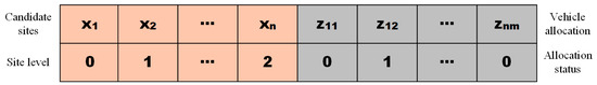
Figure 3.
Chromosome coding mode.
- Station building level coding part, where each candidate station corresponds to an integer variable , which corresponds to not building station, building level 1 station, or building level 2 station, respectively, indicating the construction status of the station.
- Vehicle assignment coding part, where each indicates whether vehicle is assigned to switching station or not, and constitutes a Boolean matrix of , which is serialized and spliced by rows.
The final chromosome is a one-dimensional vector:
- (5)
- NSGA-II performs an iterative operation where the objective function values of the individuals are quickly evaluated by the agent model.
- (6)
- For the individuals in the final non-dominating solution set, the exact value of the objective function is recalculated using the real objective function model, the solutions with large agent error are eliminated, and the Pareto frontier solution set with reliable quality is finally output.
- (7)
- Finally, the non-dominated solutions are post-processed and sorted using the TOPSIS method, and the final recommended solution is selected from the Pareto frontier solution set.
4. Calculus Analysis
4.1. Analysis of Demand for Power Switching in Operational Vehicles
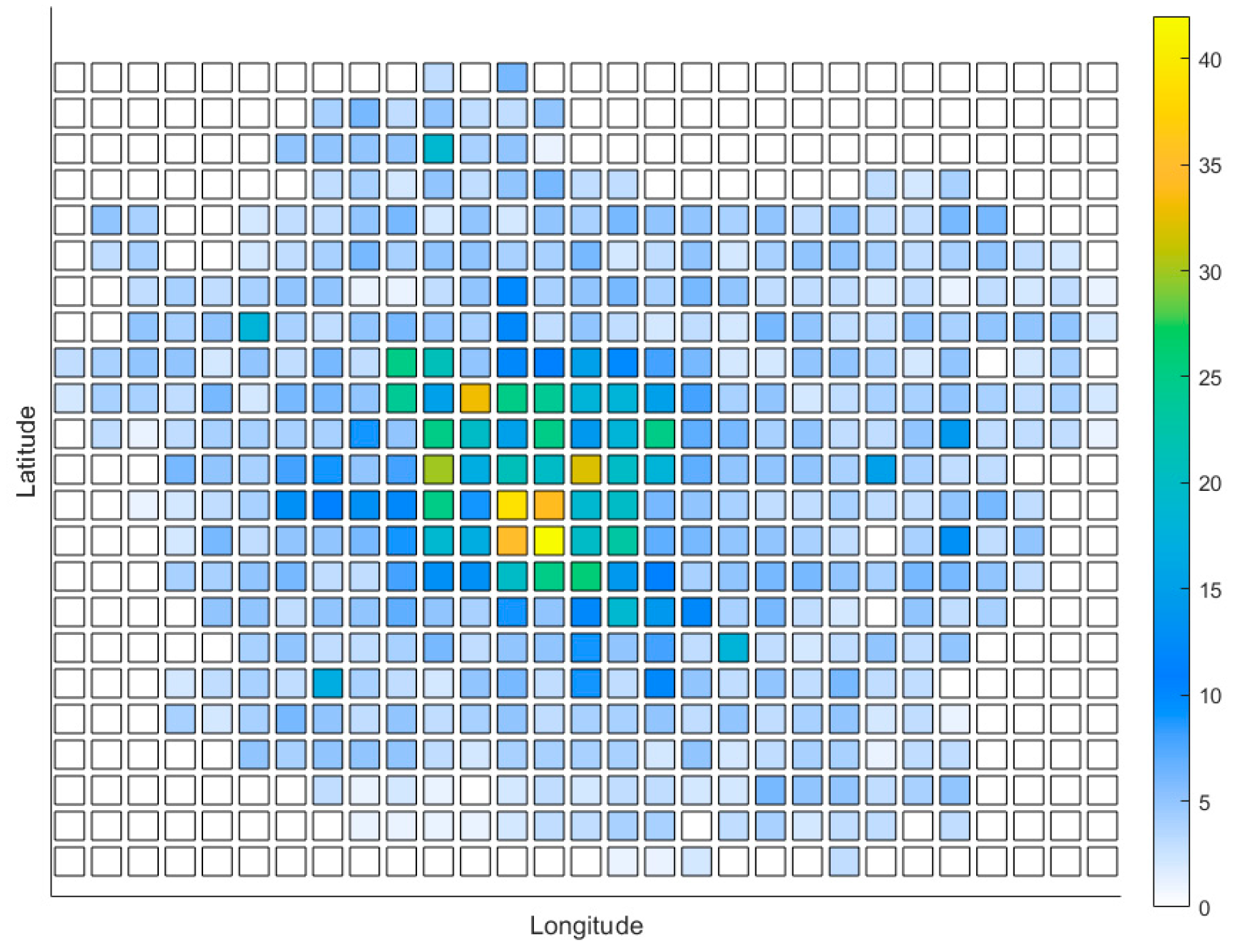
This study constructs a Monte Carlo simulation-based forecasting model for the demand for operational electric vehicle power exchange, taking the Zhangdian District of Zibo City as the empirical research scope, adopting the geographic grid discretization method to pre-process the research area, dividing the scope of the research area into a spatial grid of 1 × 1 km, and generating a total of 436 base cells, and the gridded research area is used as the basis for selecting the travel starting point of simulated journeys. The simulation area, after being divided into grids, is illustrated in Figure 4.
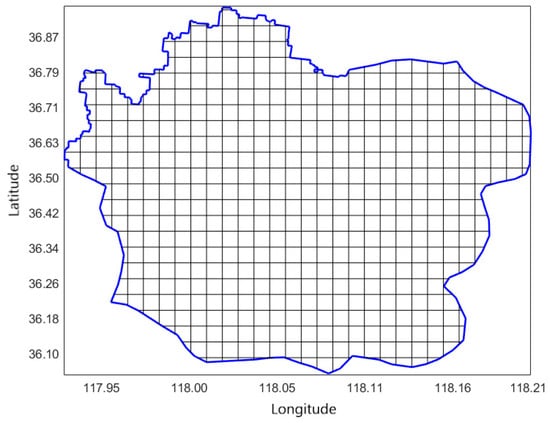
Figure 4.
Grid-based simulation area.
A simulation system containing 3000 power-switching operating vehicles was established. A typical operational EFV with the highest market share was selected as the parameter benchmark, which was equipped with a 46.08 kWh standard battery pack. The Monte Carlo algorithm was used to realize the all-weather dynamic simulation of the vehicle operation state, and through 105 random sampling iterations, the time-series distribution of battery swapping demand was obtained, as shown in Figure 5. The spatial characteristics were further visualized using a 2D kernel density map and a 3D spatiotemporal cube model, as illustrated in Figure 6.
Figure 5.
Time distribution curve of energy replenishment demand.
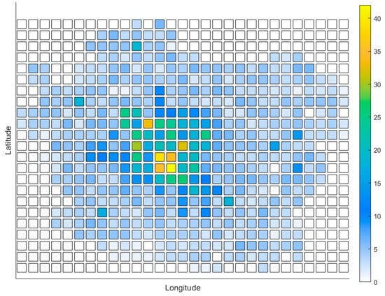
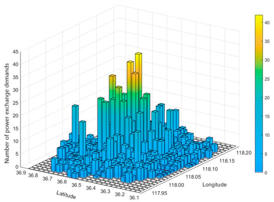
Figure 6.
Plan and stereogram of power exchange demand density.
The temporal distribution of battery swap demand revealed a distinct three-peak pattern throughout the day. A prominent morning peak occurred between 07:00 and 09:00, during which the load rapidly rose to 7500 kWh—closely aligned with the urban commuting tide—demonstrating strong spatiotemporal coupling. Although the load declined between 10:00 and 13:00, it remained at approximately 6800 kWh (about 72% of the peak value), corresponding to increased midday travel demand in central business districts. This reflects a persistent “sub-peak” pattern.
After 17:00, the load surged sharply to a daily maximum of 8272 kWh, forming the strongest peak. This fluctuation exhibited bidirectional causality with the urban congestion index, indicating high synchronization between vehicle operation, mobility demand, and energy replenishment behavior. A smaller sub-peak appeared around 22:00, with a load of 6306 kWh, consistent with the shift cycle of vehicles in economically active nighttime areas. The duration of this sub-peak was 68% shorter than the main daytime peak, reflecting the “impulse-style” energy replenishment behavior of operating vehicles.
Analyzing the two-dimensional density plan and three-dimensional cube model in the spatial dimension, the spatial distribution of the demand for power exchange in the Zhangdian District showed a significant “center-corridor agglomeration” pattern. On the whole, the hotspot area took Zibo Station as the core, and formed a spatial agglomeration pattern of biaxial diffusion along Jinjing Avenue and Liuquan Road, and the intensity of the demand for power exchange gradually decreased with the increase in the distance from the center area.
Specifically, the hotspot area was mainly built around Liuquan Road–Nanjing Road–Zhongrun Avenue to build a number of sets of crisscrossing transportation corridors, which further constitutes a rhombic high-density core area surrounded by Lutai Avenue-Changguo Road, Huaguang Road-Xincun Road, and other trunk road segments. The region gathers most of the high-frequency points of the trip of operating vehicles in the Zhangdian District, and its spatial density is highly coupled with the structure of the functional area, and the local high-density area shows obvious multi-core distribution structure, such as the southern section of Zhongrun Avenue, the west side of Lutai Avenue, and other areas, with independent peak demand for power exchange, indicating that it is difficult for a single-center-type layout mode to comprehensively cover the real demand distribution, and that it is necessary to introduce a multi-point synergistic layout strategy in the site selection planning to improve the service balance of the overall network. At the same time, the figure can also be observed in some of the edges of the region although the density is low, but there is still part of the distribution of the demand for power exchange, such as the southern industrial parks and the eastern residential areas, indicating that the subsequent planning process for the power exchange station should be in the process of guaranteeing the service capacity of the core area on the basis of the basic coverage of the edge of the region, to enhance the universality and resilience of the network.
4.2. Layout Analysis of Power Exchange Station Planning
4.2.1. Model Parameter Setting
In order to enhance the realistic adaptability and engineering feasibility of the planning and siting model of the power exchange station, the various types of cost parameters and related settings used in this paper referred to the actual construction of the power exchange station in Zhangdian District, Zibo City. The construction costs, related coefficients, and other data are shown in Table 3.
Table 3.
Costs and correlation coefficients of various factors in the model.
This article constructed a two-layer model structure that included the primary and secondary battery swapping stations. The parameter settings refer to the battery swapping station configuration scheme adopted by NIO in actual operation, as shown in Table 4.
Table 4.
Parameter settings for different levels of battery swapping stations.
4.2.2. Evaluation of Model Accuracy
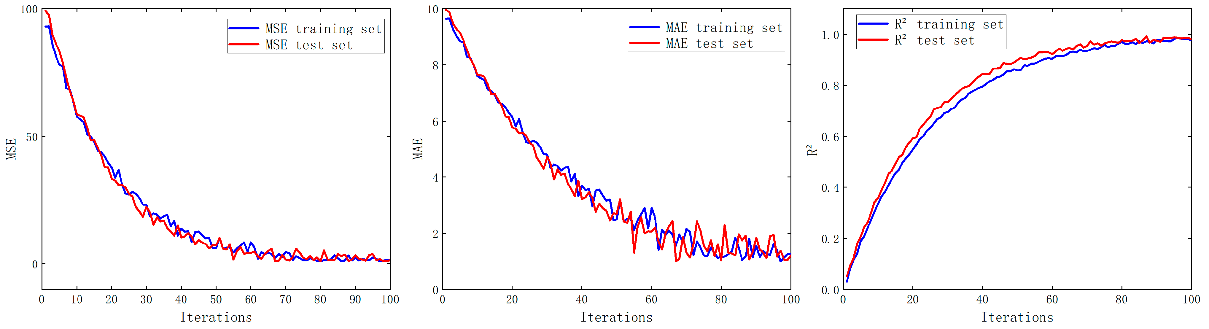
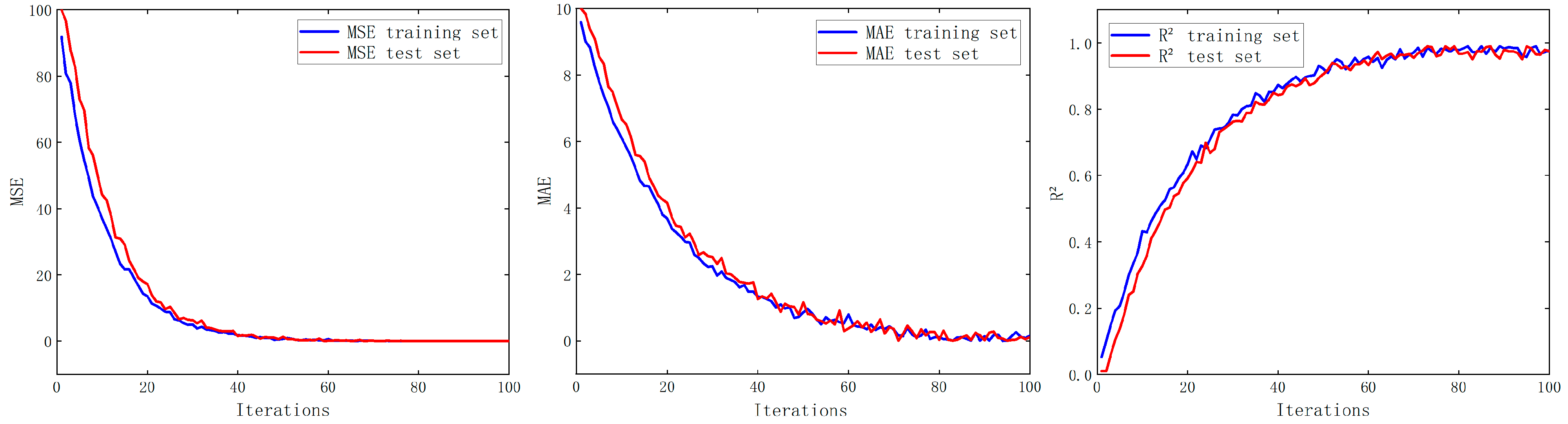
In order to evaluate the fitting accuracy of the agent model, the three metrics of Mean Square Error (MSE), Mean Absolute Error (MAE), and Coefficient of Determination (R2) were computed on the training set and validation set, respectively, in this paper. Figure 7 and Figure 8 demonstrate the dynamic trends of the three typical error metrics on the training and validation sets of the MLP agent model during the training process.
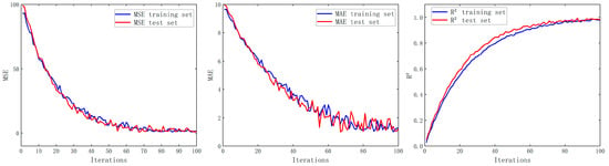
Figure 7.
Error iteration curve of MLP model for planning and construction cost.

Figure 8.
Error iteration curve of MLP model for battery swapping loss time.
Table 5 shows the errors of the model in the training process, and from the specific results, it can be seen that the training error and validation error of the MLP model on the two objective functions are at a low level, and the MAE on the validation set is about CNY 12,100 and 0.11 h, respectively, which indicates that the model has a strong generalization ability. The R2 of the construction cost model reaches 0.976, and the R2 of the lost time model is 0.971, indicating that the agent model can simulate the real objective function more accurately, and effectively replace the original model to participate in the optimization process without significant loss of accuracy.
Table 5.
MLP model training set and validation set error index values.
4.2.3. Showcase of Candidate Sites for Power Exchange Stations
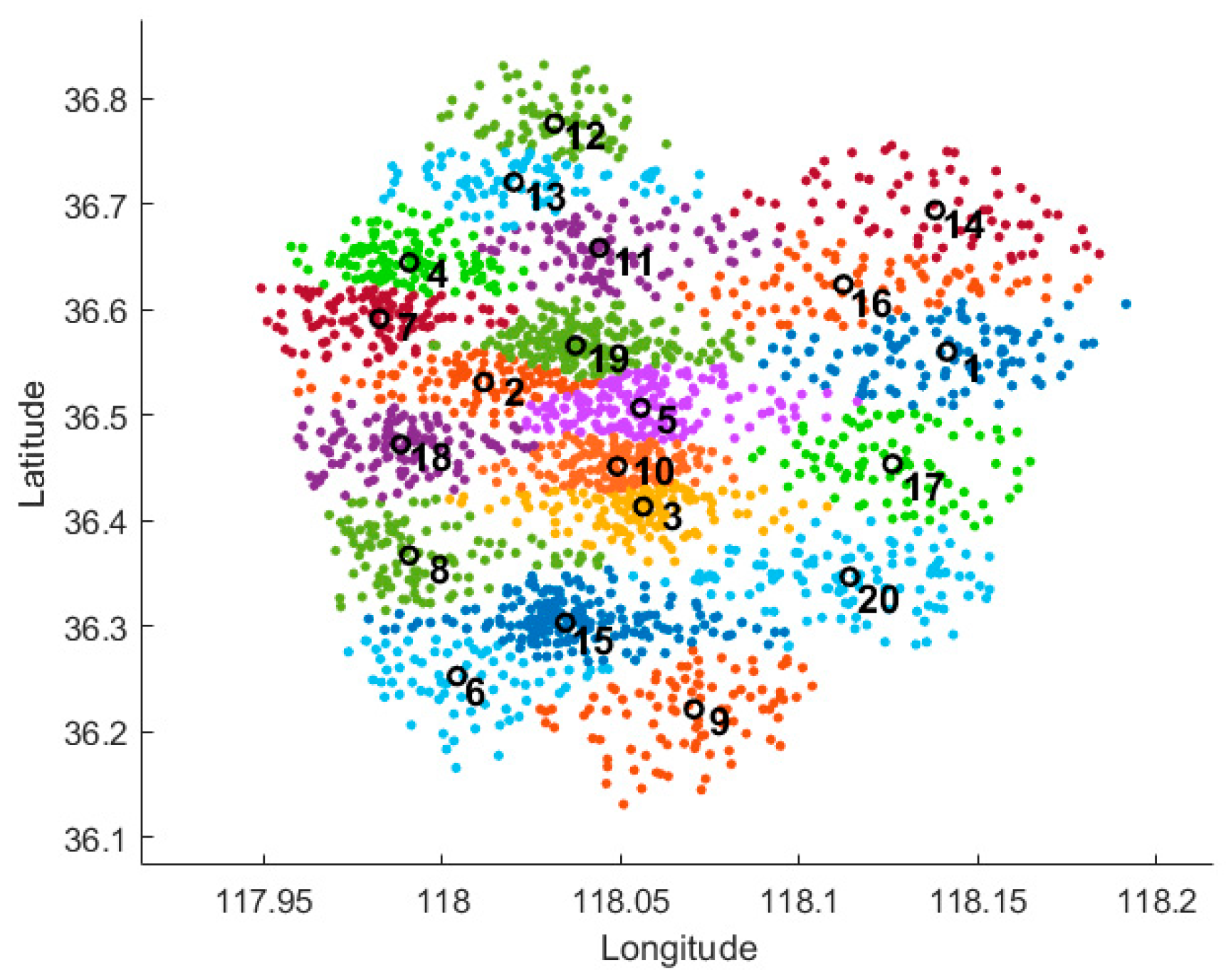
In this paper, we used a K-means clustering algorithm to jointly cluster the spatial data within the urban area based on the power exchange demand data. The optimal number of clusters K = 20 was determined by contour coefficients and other indicators, the study area was divided into 20 subregions for power exchange services, and the geometric center point of each cluster was used as the candidate station site in the region.
To enhance the practical applicability of the model’s prediction results, this study refined the K-means clustering outcomes by incorporating actual land use conditions and relevant policy constraints in the Zhangdian District. Cluster centers located in areas unsuitable for construction were removed.
To maintain the spatial continuity and demand coverage of the clustering structure, a replacement strategy was proposed for the affected clusters. Specifically, construction-feasible points were prioritized from the original sample points within each corresponding cluster to serve as new candidate centers, replacing the eliminated ones. Figure 9 shows the results of the K-means algorithm region division and the spatial visualization distribution of candidate sites.
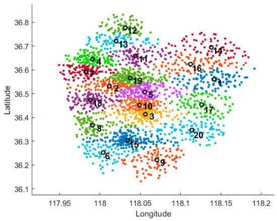
Figure 9.
Cluster distribution map of candidate sites for battery swapping stations.
4.2.4. Analysis of the Planning Results from the Integrated MLP-NSGA-II Site Selection Model
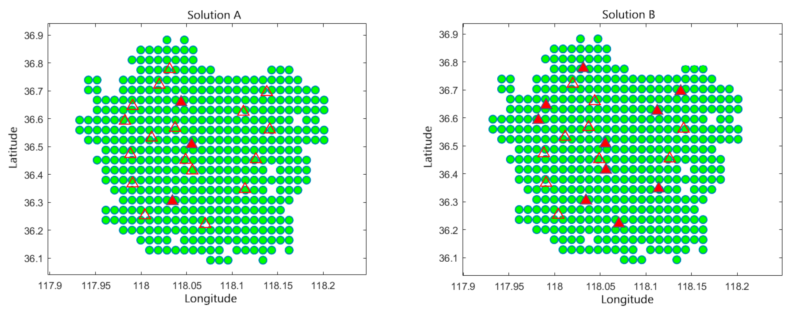
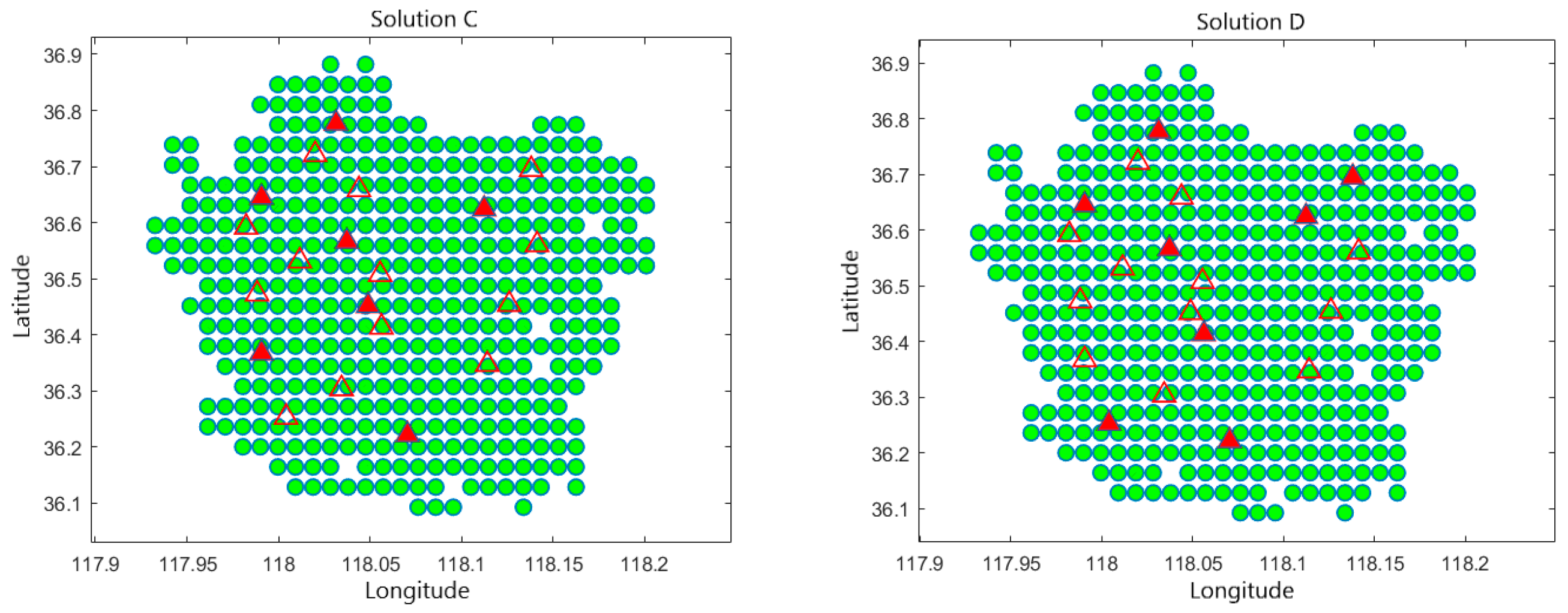
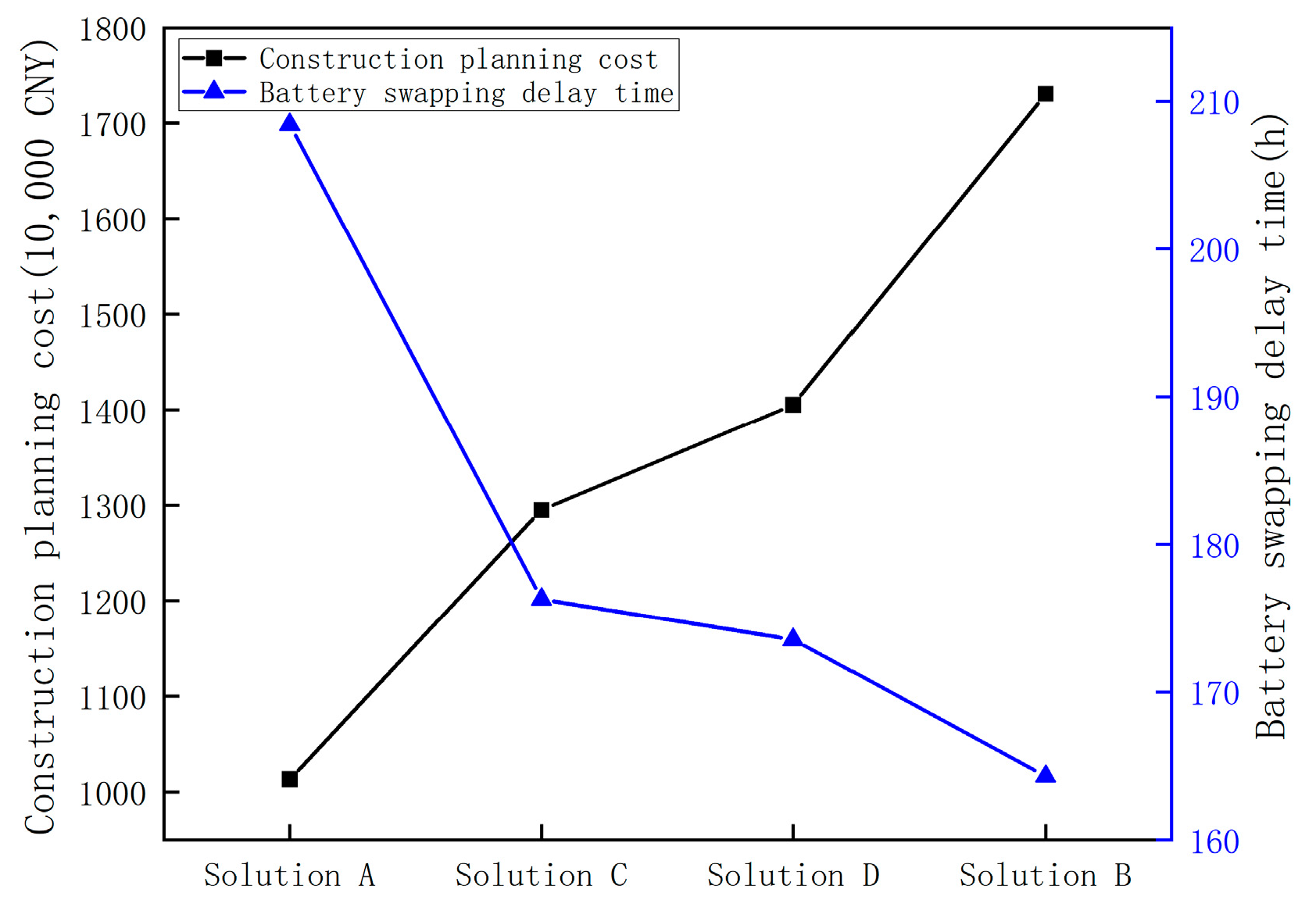
The analysis began with the Pareto non-dominated solution set obtained from the proposed method. Four representative solutions were selected from the set: (Solution A) the solution with the minimum construction cost, (Solution B) the solution with the shortest average battery swapping time, (Solution C) a balanced solution that achieves a trade-off between cost and efficiency, and (Solution D) a solution emphasizing structural diversity in spatial distribution. These four solutions reflect both extreme objective preferences and practical deployment diversity, allowing for comparative evaluation from different perspectives and application scenarios.
Table 6 presents the detailed construction locations and grade distributions of the stations for each solution. As shown in Figure 10, the visualized result of the battery swapping station location plan is presented. In the figure, red solid triangles represent the final selected stations for construction, while red hollow triangles denote unselected candidate sites. The green dots in the background indicate the spatial distribution of battery swapping demand after grid-based processing. This figure intuitively illustrates the spatial relationship between candidate site selection and demand distribution.
Table 6.
Location and level distribution of station construction for each plan.
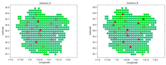

Figure 10.
Plan of site construction location for each scheme.
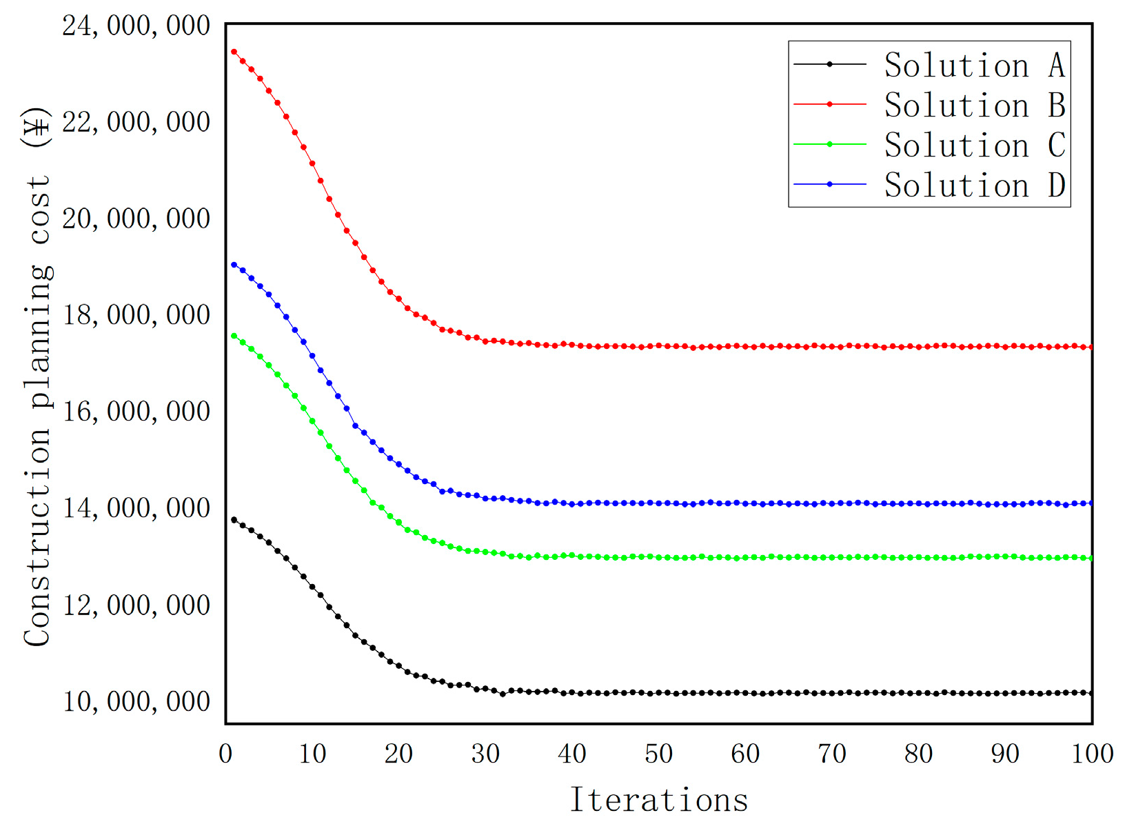
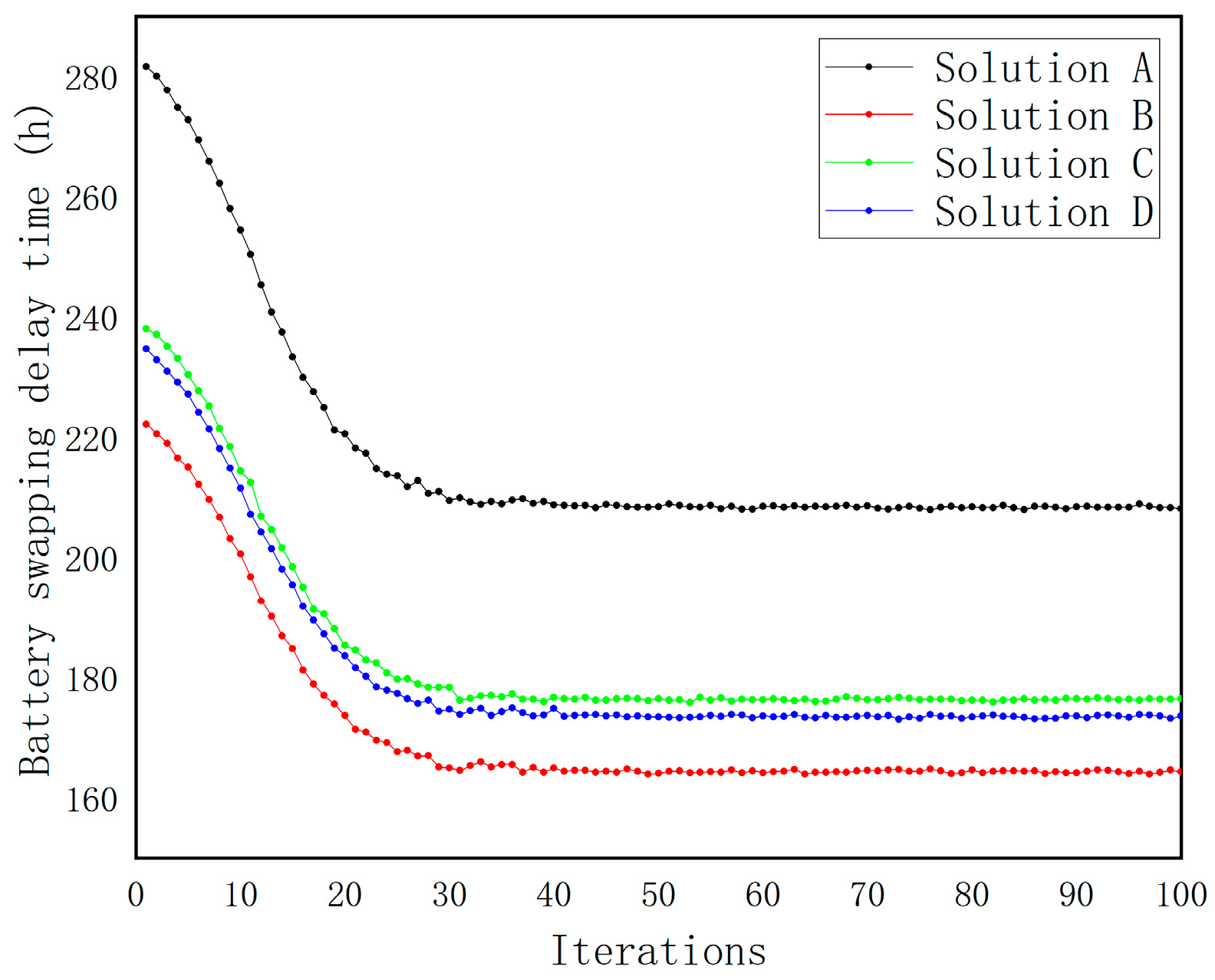
The dynamic trends of planning and construction costs versus battery swapping time loss across 100 iterations for the four representative schemes are shown in Figure 11 and Figure 12. The specific convergence data are presented in Table 7.
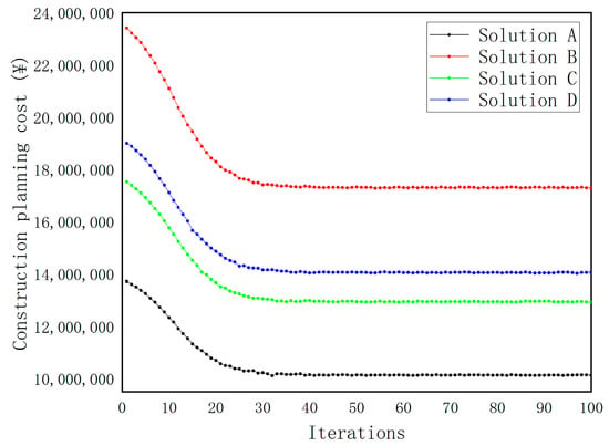
Figure 11.
Evolution trend of planning and construction costs.
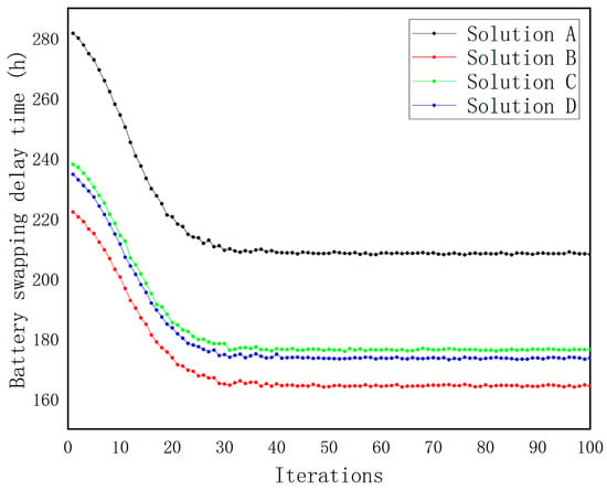
Figure 12.
Evolution trend of battery swapping loss time.
Table 7.
Comparison of indicators for construction plans of different battery swapping stations.
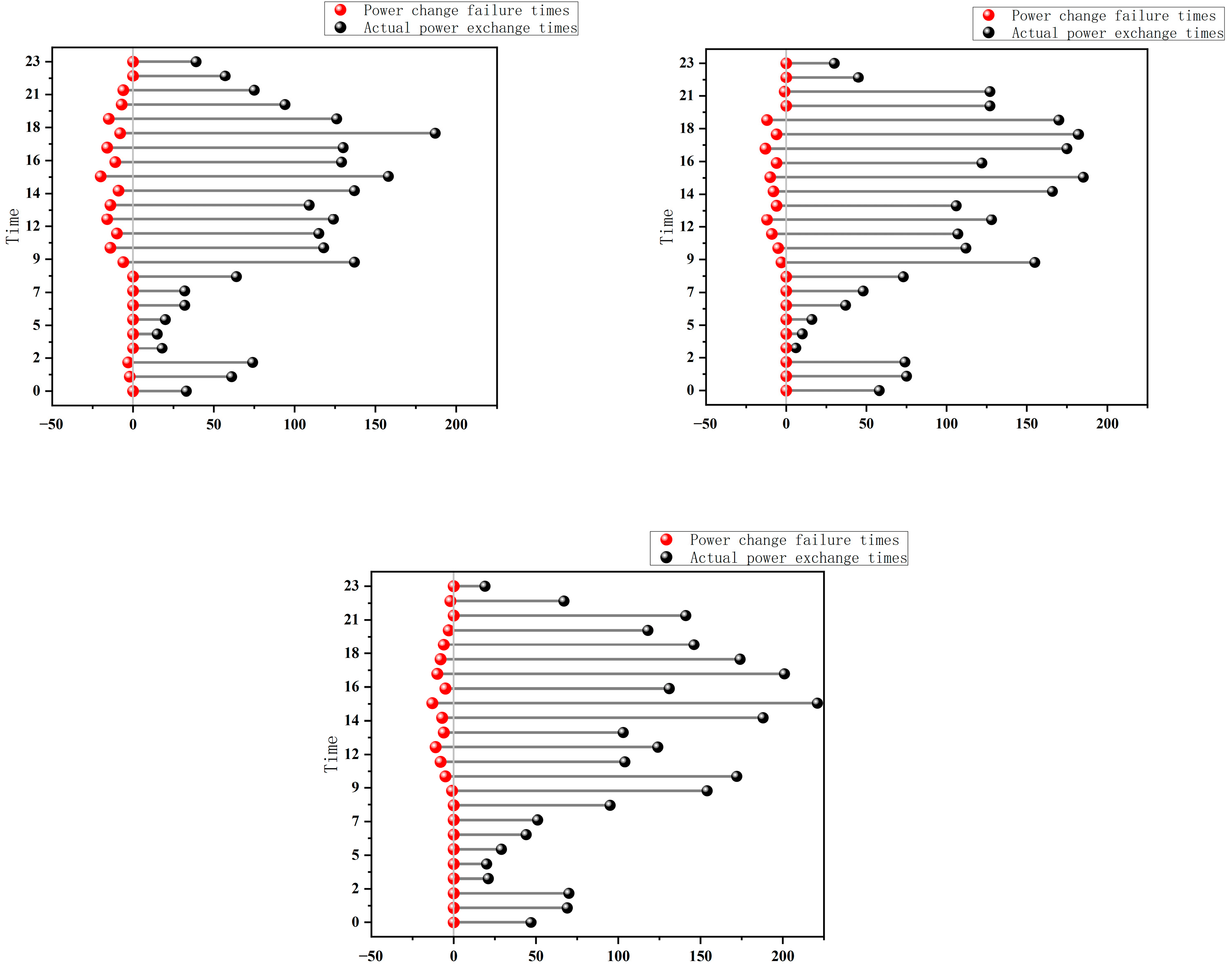
The results indicate that all four solutions experienced significant reductions in objective function values within the first 10 generations, reflecting a typical rapid convergence pattern. In Solution A, construction costs dropped swiftly from approximately CNY 1,372,000 to CNY 1,014,000. For Solution B, battery swapping delay time decreased from 222.17 h to 164.31 h, highlighting the optimization model’s high search efficiency in early iterations.
Solutions C and D also exhibited clear convergence. In Solution C, construction cost declined from CNY 1,813,000 to CNY 1,295,000, and swapping delay time from 208.95 h to 176.30 h, showing a smooth and stable trend. Solution D demonstrated strong robustness, with swapping delay time falling rapidly in the first 10 generations and stabilizing around 173.53 h after the 40th generation. Its construction cost also decreased steadily from CNY 1,907,000 to CNY 1,425,000, with minimal fluctuation.
Overall, the objective functions of all four solutions converged around the 40th generation, with only slight variations thereafter. This confirms that the integrated MLP-NSGA-II algorithm achieves both high optimization quality and fast convergence speed. Throughout the convergence process, local fluctuations of the objective values remained within a reasonable range. In particular, Solutions C and D demonstrated high stability in the middle and later stages, further validating the robustness and convergence performance of the proposed MLP-NSGA-II approach. The comparison of objective function values across different schemes is illustrated in Figure 13.
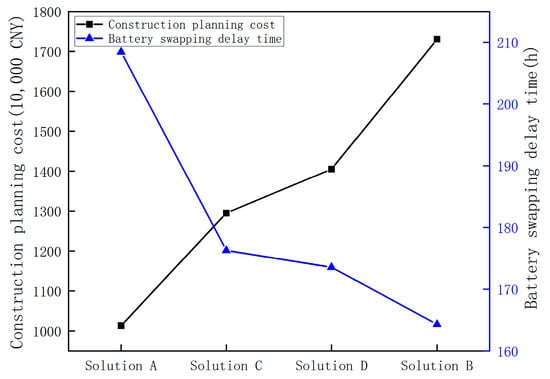
Figure 13.
Comparison of planning and construction costs and replacement loss time for different site selection plans.
The TOPSIS method was applied to comprehensively evaluate the ideality of the four representative solutions. Although Solution A excelled in cost control, its relatively low service efficiency resulted in a lower overall score. Solution B achieved the best performance in minimizing battery swapping delay time, but its significantly higher construction cost reduced its overall ranking. Solution D showed a more balanced performance, with a score of 0.72. Solution C demonstrated strong results in both objectives, achieving the highest composite score of 0.74, reflecting its excellent balance between construction cost and service efficiency.
Considering the performance and evaluation outcomes of all the solutions, this study ultimately selects Solution C as the recommended battery swapping station site selection plan based on the integrated MLP-NSGA-II optimization algorithm.
4.2.5. Comparative Analysis of Site Planning Results
In order to verify the superiority of the proposed MLP-NSGA-II joint optimization method, this paper selects the traditional genetic algorithm (GA) and the Density Peak Clustering (DPC) algorithm as the comparison method. Both of them are contrasted with the main model in terms of optimization idea, result expression, and applicability to verify the comprehensive performance of the main algorithm from multiple dimensions.
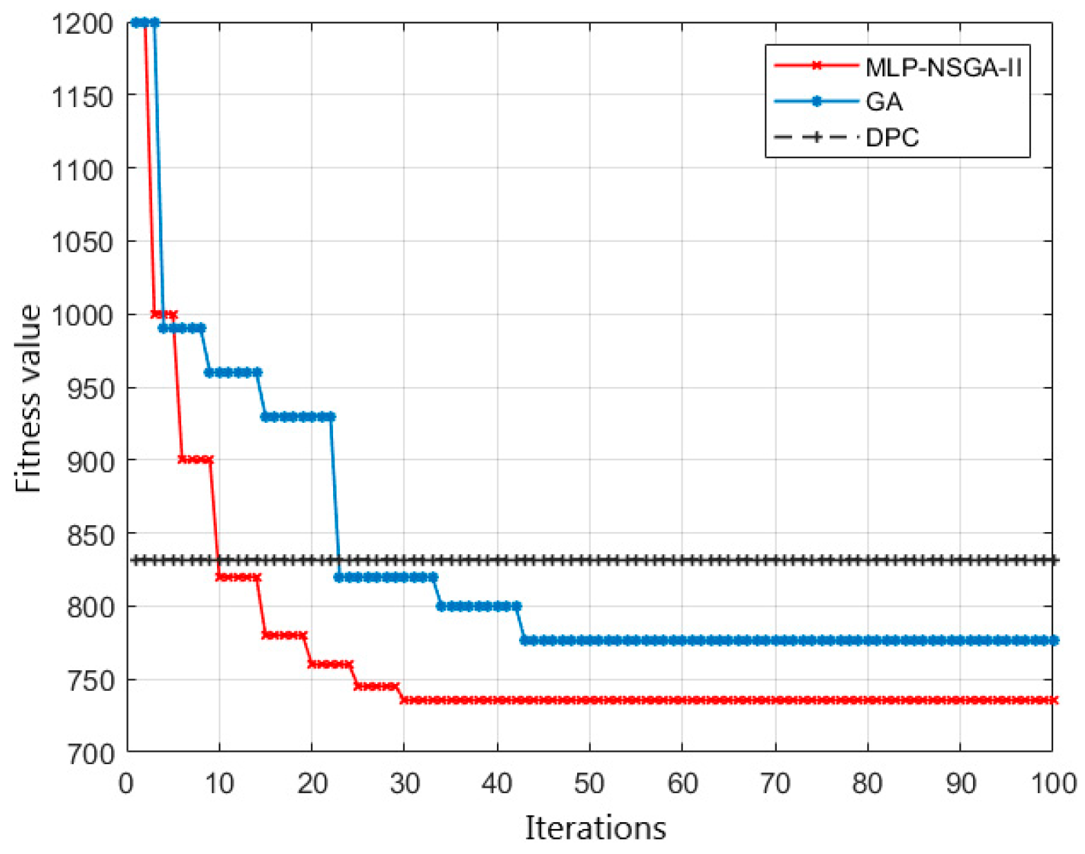
The genetic algorithm adopts a weighted sum approach to combine multiple objectives into a single-objective function for optimization. As a heuristic method, GA has been widely applied in complex combinatorial problems such as electric vehicle charging station location planning [36,37]. On the other hand, the Density Peak Clustering method, as an unsupervised clustering approach [38], has been extensively used in urban spatial analysis and preliminary infrastructure site screening, representing an empirical siting strategy under non-optimization models. A comparison of the convergence curves for different algorithms is shown in Figure 14.
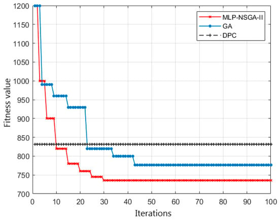
Figure 14.
Iterative fitness curves of MLP-NSGA-II, GA, and DPC algorithms.
The convergence curve demonstrates that the MLP-NSGA-II joint algorithm outperforms the traditional genetic algorithm (GA) in both optimization speed and convergence stability. The proposed method achieves convergence by the 30th iteration, with the objective function value stabilizing thereafter. In contrast, GA reaches a stable state at the 43rd iteration, indicating a convergence speed approximately 30.23% slower than MLP-NSGA-II. Additionally, the final fitness value obtained by GA is about 9.5% higher than that of the joint algorithm, reflecting inferior solution quality.
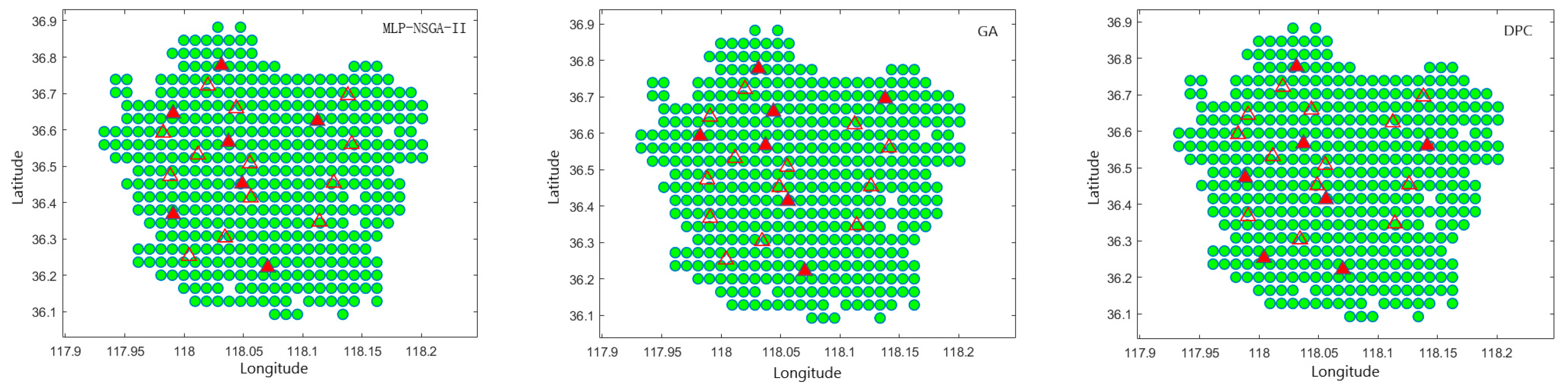
Figure 15 presents the optimal station siting schemes derived from the MLP-NSGA-II, GA, and DPC methods. For the DPC approach, supplementary constraints are introduced to regulate station scale and spatial layout. Specifically, the top seven cluster centers—selected based on demand density and spatial representativeness—are designated as station locations. To avoid excessive clustering and overlapping service areas, a minimum inter-station distance threshold is enforced. These adjustments align the DPC method with the optimization-based approaches in terms of station count and spatial distribution while preserving its intrinsic clustering logic.
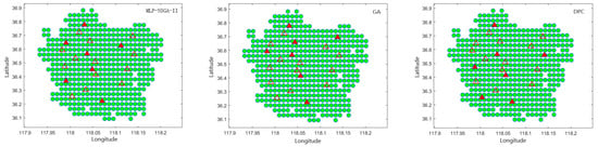
Figure 15.
MLP-NSGA-II, GA, and DPC construction plan site location plan schematic diagram.
Overall, the three approaches exhibit significant differences in site selection strategy, spatial distribution, and station hierarchy. As summarized in Table 8, all the approaches select seven stations, yet their hierarchical configurations differ markedly. The MLP-NSGA-II scheme locates secondary stations near high-demand grids within the urban core, forming a “strong center response” layout that emphasizes service efficiency in dense areas. The GA method presents a more dispersed configuration, with some secondary stations positioned outside core zones, reflecting weaker demand alignment. The DPC method, while achieving broader spatial coverage, lacks hierarchical optimization; its station distribution along major roads limits allocation efficiency and reduces responsiveness to localized demand patterns.
Table 8.
MLP-NSGA-II, GA, and DPC construction plan site construction location.
To enable a fair comparison of the optimal site selection schemes from the three algorithms, two auxiliary indicators—service coverage and power exchange service utilization—were introduced in the post-evaluation stage. Since the DPC method does not optimize an explicit objective function, it cannot directly account for operational metrics such as power exchange time loss. These indicators allowed for a consistent evaluation of spatial coverage and service efficiency across all three methods, including MLP-NSGA-II and GA.
- (1)
- The coverage ratio of power exchange service is the ratio of the number of power exchange demand points effectively covered by the service radius of a power exchange station to the total number of demand points. If the distance from a demand point to any power exchange station is less than the service radius of the power exchange station, it is considered to be covered, and the formula is as follows:
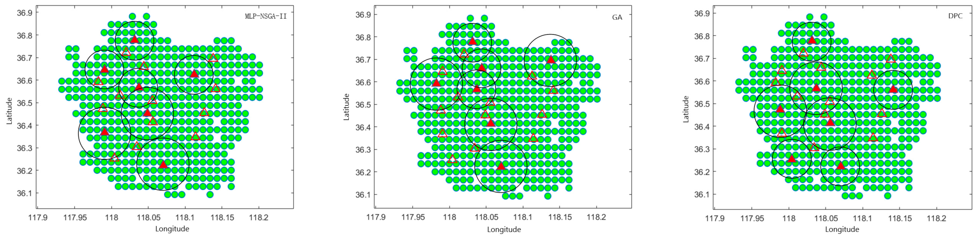
The corresponding power exchange service coverage for each scenario is shown in Figure 16. In this case, each diagram is centered on the built site, the service coverage area is plotted according to the service radius set by the site level, and the location of all power exchange demand points is superimposed.
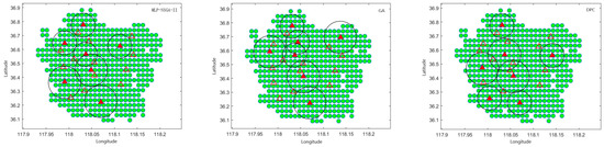
Figure 16.
MLP-NSGA-II, GA, and DPC construction plan site battery swapping service scope.
Table 9 presents the number of demand points covered by each scheme under the service radius constraint. The coverage rates for the MLP-NSGA-II, GA, and DPC methods are 94.30%, 88.96%, and 82.19%, respectively. Among them, the MLP-NSGA-II scheme achieves the highest coverage, with only 154 demand points remaining uncovered. This indicates a more spatially balanced station layout, effectively targeting high-density demand clusters. The GA method ranks second, though it still exhibits partial service gaps in lower-density or peripheral areas. In contrast, the DPC approach yields the lowest coverage rate; its stations are primarily concentrated along major urban roads, resulting in dense coverage within central clusters but limited spatial reach toward peripheral zones, reflecting poor service scalability.
Table 9.
Coverage of battery swapping services for MLP-NSGA-II, GA, and DPC construction plans.
- (2)
- The utilization rate of power exchange service , which is the ratio of the actual number of completed power exchanges of the power exchange station to its theoretical maximum service capacity under the specified service capacity limit, reflects the utilization efficiency of the station’s resources in all-day operation, and is calculated by the formula:
The results of planning and construction cost and switching service utilization of different algorithmic optimal siting schemes are shown in Table 10. Meanwhile, combining with the simulation of switching service allocation, the distribution of switching service states of each algorithmic optimal scheme under all-day operation conditions is derived, as shown in Figure 17.
Table 10.
Comparison of service utilization rates for MLP-NSGA-II, GA, and DPC construction plans.
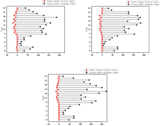
Figure 17.
All-day service status of DPC, GA, and MLP-NSGA-II site selection scheme.
Comparing the coverage and utilization rates of the different schemes, the joint optimization strategy based on MLP-NSGA-II shows the best overall performance, with a service coverage of 94.30%, which is 12.11% higher than that of DPC, and a service utilization rate of 85.35%, which is 6.25% and 19.69% higher than that of GA and DPC, respectively. The results show that the MLP-NSGA-II scheme is more coordinated in terms of station hierarchy, spatial layout, and load matching, and has the best service efficiency; the GA method is the second best; and the DPC method has the lowest service utilization rate, reflecting that there is significant room for improvement in spatial allocation and resource regulation.
The above analysis shows that under the constraints of the same construction scale and the number of stations, the joint optimization strategy based on MLP-NSGA-II is able to reasonably configure the primary and secondary power exchange stations on the basis of fully considering the spatial structure of the city and the distribution of the power exchange demand, realizing the hierarchical response of the core and peripheral areas, and effectively improving the utilization efficiency of the station’s service capacity and the overall service completion rate, and showing better service efficiency and overall service completion rate in the siting problem of the power exchange station. It effectively improves the utilization efficiency of station service capacity and the overall service completion rate, and shows better global performance and application potential in the siting problem of power exchange stations.
5. Conclusions
In order to realize the efficient matching between the demand for power exchange of urban operating vehicles and the supply capacity of regional power exchange infrastructure, and to take into account the operating efficiency of vehicles and the planning and construction cost of power exchange stations, this paper proposes a strategy for planning the appropriate number and level of power exchange station layout according to the need from the service capacity of different levels of power exchange facilities, so as to meet the diversified replenishment demand in the region. Based on the above research objectives, the main research results of this paper include the following:
- (1)
- By extracting and analyzing the real-vehicle trajectory dataset in Zibo City, we completed the modeling and analysis of the operating characteristic laws, including the trip distance, trip destination, the distribution of departure starting moments, and the state of energy consumption, so as to provide probabilistic decision-making benchmarks for the accurate prediction of power exchange loads.
- (2)
- The modeling and prediction of the demand for power exchange of operating vehicles were based on a three-layer prediction architecture consisting of “grid-based travel space modeling–probabilistic travel feature portrayal–Monte Carlo stochastic simulation”, which dynamically simulates the trajectory of the vehicles and deduces the spatial and temporal evolution characteristics of the regional demand for power exchange. The three-layer prediction architecture consisted of “grid-based travel space modeling, probabilistic travel feature portrayal, and Monte Carlo stochastic simulation”.
- (3)
- A multi-objective hierarchical siting optimization model was constructed for the problem of siting optimization of power exchange stations in urban areas, taking into account the station hierarchy, construction cost, and power exchange loss time simultaneously. In order to achieve an efficient solution, a joint optimization method framework combining MLP-NSGA-II was proposed and compared with the GA and DPC method. The results show that MLP-NSGA-II significantly outperforms the traditional method in terms of optimization efficiency and solution set quality, with an improvement of about 30.23% in convergence speed, and an improvement of 6.25% and 19.69% compared to the GA model site selection scheme and the traditional DPC method site selection scheme, respectively. The joint optimization model proposed in this paper has significant advantages in improving the coverage capacity, optimizing the resource allocation efficiency, and enhancing the service response performance, which provides practical modeling paths and decision-making references for the scientific layout of city-level power exchange infrastructure.
This study takes the Zhangdian District of Zibo City as the case study area. The local road network features a primarily regular grid structure, complemented by radial roads in some sections, making it representative of urban road systems. This “grid + radial” pattern is widely observed in many medium- and large-sized Chinese cities, such as Jinan, Zhengzhou, and Tangshan, thus enhancing the generalizability of using Zhangdian as a typical study area.
Furthermore, the proposed battery swapping demand forecasting method and the integrated MLP-NSGA-II optimization framework are designed to depend on general parameters—such as spatial demand distribution and service radius—without imposing specific assumptions about the underlying road network structure. This design ensures strong regional adaptability and transferability, making the method applicable to other urban environments with different traffic configurations.
6. Future Work and Research Outlook
At present, the model validation in this study still has certain limitations due to the lack of detailed operational data for battery swapping stations. The prediction results are primarily based on a battery swapping demand forecasting method constructed through travel chain analysis and Monte Carlo simulation, without empirical verification using actual swapping behavior data. Future research will focus on incorporating real-world operational data to systematically evaluate and refine the model’s predictive performance. An overview of research progress and a specific comparison of future improvement directions are shown in Table 11.
Table 11.
Summary of research development and future improvements.
In addition, the current model does not fully account for the influence of data types, such as holidays or special events, on battery swapping demand. During these periods, the operating characteristics of electric vehicles may shift significantly, with vehicle travel patterns and energy replenishment needs showing notable heterogeneity. Therefore, future research could further refine the model by integrating the temporal variations in vehicle behavior associated with holiday seasons.
Author Contributions
Conceptualization, P.M.; data curation, S.Z., W.S., and H.L.; formal analysis, S.Z. and B.Z.; investigation, W.S. and H.L.; methodology, P.M.; project administration, D.G.; resources, B.Z.; validation, T.M.; visualization, T.M.; writing—original draft, P.M.; writing—review and editing, P.M. and D.G. All authors have read and agreed to the published version of the manuscript.
Funding
It is sponsored by the State Key Lab of Intelligent Transportation System under Project No. 2024-B009, the National Nature Science Foundation of China No.52102465, and Shandong Provincial Nature Science Foundation of China No. ZR2021MG012. We appreciate the financial support from the SDUT & Zibo City Integration Development Project (Grant No.2022JS005).
Data Availability Statement
The original contributions presented in the study are included in the article, further inquiries can be directed to the corresponding author.
Conflicts of Interest
The authors declare no conflict of interest.
References
- Ahmad, F.; Saad Alam, M.; Saad Alsaidan, I.; Shariff, S.M. Battery swapping station for electric vehicles: Opportunities and challenges. IET Smart Grid 2020, 3, 280–286. [Google Scholar] [CrossRef]
- IEA. World Energy Outlook 2023 [EB/OL]; IEA: Paris, France; Available online: https://www.iea.org/reports/world-energy-outlook-2023 (accessed on 25 March 2023).
- Basu, M. Sustainable power, heat and natural gas scheduling of remote microgrid incorporating battery swapping station and fuel constraints. Int. J. Hydrogen Energy 2024, 91, 1315–1329. [Google Scholar] [CrossRef]
- Fuchs, I.; Sanchez-Solis, C.; Balderrama, S.; Valkenburg, G. Swarm electrification for Raqaypampa: Impact of different battery control setpoints on energy sharing in interconnected solar homes systems. Sustain. Energy Grids Netw. 2024, 40, 101535. [Google Scholar] [CrossRef]
- Afshar, M.; Mohammadi, M.R.; Abedini, M. A novel spatial–temporal model for charging plug hybrid electrical vehicles based on traffic-flow analysis and Monte Carlo method. ISA Trans. 2021, 114, 263–276. [Google Scholar] [CrossRef] [PubMed]
- Su, J.; Lie, T.T.; Zamora, R. Modelling of large-scale electric vehicles charging demand: A New Zealand case study. Electr. Power Syst. Res. 2019, 167, 171–182. [Google Scholar] [CrossRef]
- Lin, H.; Fu, K.; Wang, Y.; Sun, Q.; Li, H.; Hu, Y.; Sun, B.; Wennersten, R. Characteristics of electric vehicle charging demand at multiple types of location-Application of an agent-based trip chain model. Energy 2019, 188, 116122. [Google Scholar] [CrossRef]
- Zhang, L.; Huang, Z.; Wang, Z.; Li, X.; Sun, F. An urban charging load forecasting model based on trip chain model for private passenger electric vehicles: A case study in Beijing. Energy 2024, 299, 130844. [Google Scholar] [CrossRef]
- Li, Y.; Su, S.; Liu, B.; Yamashita, K.; Li, Y.; Du, L. Trajectory-driven planning of electric taxi charging stations based on cumulative prospect theory. Sustain. Cities Soc. 2022, 86, 104125. [Google Scholar] [CrossRef]
- Gao, K.; Sun, L.; Yang, Y.; Meng, F.; Qu, X. Cumulative prospect theory coupled with multi-attribute decision making for modeling travel behavior. Transp. Res. Part A Policy Pract. 2021, 148, 1–21. [Google Scholar] [CrossRef]
- Yi, Z.; Liu, X.C.; Wei, R.; Chen, X.; Dai, J. Electric vehicle charging demand forecasting using deep learning model. J. Intell. Transp. Syst. 2022, 26, 690–703. [Google Scholar] [CrossRef]
- Feng, J.; Yang, J.; Li, Y.; Wang, H.; Ji, H.; Yang, W.; Wang, K. Load forecasting of electric vehicle charging station based on grey theory and neural network. Energy Rep. 2021, 7, 487–492. [Google Scholar] [CrossRef]
- Wang, S.; Chen, A.; Wang, P.; Zhuge, C. Short-term electric vehicle battery swapping demand prediction: Deep learning methods. Transp. Res. Part D Transp. Environ. 2023, 119, 103746. [Google Scholar] [CrossRef]
- Shalaby, A.A.; Shaaban, M.F.; Mokhtar, M.; Zeineldin, H.H.; El-Saadany, E.F. A dynamic optimal battery swapping mechanism for electric vehicles using an LSTM-based rolling horizon approach. IEEE Trans. Intell. Transp. Syst. 2022, 23, 15218–15232. [Google Scholar] [CrossRef]
- Yan, Q.; Lin, H.; Li, J.; Ai, X.; Shi, M.; Zhang, M.; Gejirifu, D. Many-objective charging optimization for electric vehicles considering demand response and multi-uncertainties based on Markov chain and information gap decision theory. Sustain. Cities Soc. 2022, 78, 103652. [Google Scholar] [CrossRef]
- Wu, C.; Jiang, S.; Gao, S.; Liu, Y.; Han, H. Charging demand forecasting of electric vehicles considering uncertainties in a microgrid. Energy 2022, 247, 123475. [Google Scholar] [CrossRef]
- Sheng, Y.; Guo, Q.; Liu, M.; Lan, J.; Zeng, H.; Wang, F. User charging behavior analysis and charging facility planning practice based on multi-source data fusion. Autom. Electr. Power Syst. 2022, 46, 151–162. [Google Scholar]
- Zhang, M.; Xu, L.; Yang, X. EV charging demand prediction based on city grid attribute division. Electr. Meas. Instrum. 2025, 62, 10–19. [Google Scholar]
- Liu, L.; Wu, T.; Chen, X.; Zheng, W.; Xu, Q. Multi-objective optimal allocation of DG and EV charging station based on space-time characteristics and demand response. Electr. Power Autom. Equip. 2021, 41, 48–56. [Google Scholar]
- Wolbertus, R.; Kroesen, M.; van den Hoed, R.; Chorus, C. Fully charged: An empirical study into the factors that influence connection times at EV-charging stations. Energy Policy 2018, 123, 1–7. [Google Scholar] [CrossRef]
- Li, Y.; Pei, W.; Zhang, Q.; Xu, D.; Ma, H. Optimal layout of electric vehicle charging station locations considering dynamic charging demand. Electronics 2023, 12, 1818. [Google Scholar] [CrossRef]
- Yi, Z.; Liu, X.C.; Wei, R. Electric vehicle demand estimation and charging station allocation using urban informatics. Transp. Res. Part D Transp. Environ. 2022, 106, 103264. [Google Scholar] [CrossRef]
- Hou, H.; Wang, Y.; Huang, L.; Chen, Y.; Xie, C.; Zhang, R. Charging optimization strategy of composite charging station with energy storage to meet fast charging demand of electric vehicles. Electr. Power Autom. Equip. 2022, 42, 65–71. [Google Scholar]
- He, Y.; Guo, S.; Zhou, J.; Wu, F.; Huang, J.; Pei, H. The quantitative techno-economic comparisons and multi-objective capacity optimization of wind-photovoltaic hybrid power system considering different energy storage technologies. Energy Convers. Manag. 2021, 229, 113779. [Google Scholar] [CrossRef]
- Wang, J.; Xue, K.; Guo, K.; Ma, J.; Zhou, X.; Liu, M.; Yan, J. Multi-objective capacity programming and operation optimization of an integrated energy system considering hydrogen energy storage for collective energy communities. Energy Convers. Manag. 2022, 268, 116057. [Google Scholar] [CrossRef]
- Zhang, B.; Yan, Q.; Zhang, H.; Zhang, L. Optimization of Charging/Battery-Swap Station Location of Electric Vehicles with an Improved Genetic Algorithm-BasedModel. CMES-Comput. Model. Eng. Sci. 2023, 134, 1177–1194. [Google Scholar]
- He, Y.; Zhang, Y.; Fan, T.; Cai, X.; Xu, Y. The charging station and swapping station site selection with many-objective evolutionary algorithm. Appl. Intell. 2023, 53, 18041–18060. [Google Scholar] [CrossRef]
- Zhang, Y.; Luo, X.; Qiu, Y.; Fu, Y. Understanding the generation mechanism of BEV drivers’ charging demand: An exploration of the relationship between charging choice and complexity of trip chaining patterns. Transp. Res. Part A Policy Pract. 2022, 158, 110–126. [Google Scholar] [CrossRef]
- Xing, Q.; Chen, Z.; Huang, X.; Zhang, Z.; Leng, Z.; Xu, Y.; Zhao, Q. Electric vehicle charging demand forecasting model based on data driven mode. Proc. CSEE 2020, 40, 3796–3813. [Google Scholar]
- Ma, X.; Li, Y.; Wang, H.; Wang, C.; Hong, X. Research on demand of charging piles based on stochastic simulation of EV trip chain. Trans. China Electrotech. Soc. 2017, 32 (Suppl. S2), 190–202. [Google Scholar]
- CJJ.37-2015—2012; Code for Design of Urban Road Engineering. China Construction Industry Press: Beijing, China, 2012.
- Gao, Q.; Lin, Z.; Zhu, T.; Zhou, W.; Wang, G.; Zhang, T.; Zhang, Z.; Waseem, M.; Liu, S.; Han, C.; et al. Charging Load Forecasting of Electric Vehicle Based on Monte Carlo and Deep Learning. In Proceedings of the 2019 IEEE Sustainable Power and Energy Conference (iSPEC), Beijing, China, 21–23 November 2019. [Google Scholar]
- Xing, Y.; Li, F.; Sun, K.; Wang, D.; Chen, T.; Zhang, Z. Multi-type electric vehicle load prediction based on Monte Carlo simulation. Energy Rep. 2022, 8, 966–972. [Google Scholar] [CrossRef]
- Cordeiro-Costas, M.; Labandeira-Pérez, H.; Villanueva, D.; Pérez-Orozco, R.; Eguía-Oller, P. NSGA-II based short-term building energy management using optimal LSTM-MLP forecasts. Int. J. Electr. Power Energy Syst. 2024, 159, 12. [Google Scholar] [CrossRef]
- Bocoum, A.O.; Rasaei, M.R. Multi-objective optimization of WAG injection using machine learning and data-driven Proxy models. Appl. Energy 2023, 349, 10. [Google Scholar] [CrossRef]
- Zhou, G.; Zhu, Z.; Luo, S. Location optimization of electric vehicle charging stations: Based on cost model and genetic algorithm. Energy 2022, 247, 123437. [Google Scholar] [CrossRef]
- Choi, M.; Van Fan, Y.; Lee, D.; Kim, S.; Lee, S. Location and capacity optimization of EV charging stations using genetic algorithms and fuzzy analytic hierarchy process. Clean Technol. Environ. Policy 2025, 27, 1785–1798. [Google Scholar] [CrossRef]
- Xiao, S.; Zhou, Z.; Chen, Z.; Qi, Y. Bus Station Location Selection Method Based on DBSCAN-DPC Clustering Algorithm. In International Conference on Autonomous Unmanned Systems; Springer Nature: Singapore, 2023; pp. 140–150. [Google Scholar]


Disclaimer/Publisher’s Note: The statements, opinions and data contained in all publications are solely those of the individual author(s) and contributor(s) and not of MDPI and/or the editor(s). MDPI and/or the editor(s) disclaim responsibility for any injury to people or property resulting from any ideas, methods, instructions or products referred to in the content. |
© 2025 by the authors. Published by MDPI on behalf of the World Electric Vehicle Association. Licensee MDPI, Basel, Switzerland. This article is an open access article distributed under the terms and conditions of the Creative Commons Attribution (CC BY) license (https://creativecommons.org/licenses/by/4.0/).