State-Space Method-Based Frame Dynamics Analysis of the Six-Rotor Unmanned Aerial Vehicles

Abstract

As a key component of unmanned aerial vehicles (UAVs), the vibrational characteristics of the airframe critically impact flight safety and imaging quality. These vibrations, often generated by motor-propeller systems or aerodynamic forces, can lead to structural fatigue during flight or cause image blur in payloads like cameras. To analyze the dynamic performance of the six-rotor UAV frame, this paper develops a state-space model based on linear state-space theory, structural dynamics principles, and modal information. The Direct Current (DC) gain method is employed to reduce the number of modes, followed by frequency response analysis on the reduced modes to derive the frequency–domain transfer function between the excitation input and response output points. The contribution of each mode to the overall frequency response is evaluated, and the frequency response curve is subsequently plotted. The results indicate that the model achieves a 73-fold speed improvement with an error rate of less than 13%, thereby validating the accuracy of the six-rotor UAV frame state-space model. Furthermore, the computational efficiency has been significantly enhanced, meeting the requirements for vibration simulation analysis. The dynamic analysis approach grounded in state-space theory offers a novel methodology for investigating the dynamic performance of complex structures, enabling efficient and precise analysis of frequency response characteristics in complex linear systems such as electric vehicle (EV) battery modules and motor systems. By treating EV components as dynamic systems with coupled mechanical–electrical interactions, this method contributes to the reliability and safety of sustainable transportation systems, addressing vibration challenges in both UAVs and EVs through unified modeling principles.

1. Introduction

China has consistently ranked as the world’s leading exporter of civilian unmanned aerial vehicles (UAVs) for many years. The country accounts for over 70% of global patent applications in the UAV sector, positioning it as the foremost technology originator. In recent years, China’s UAV industry has achieved substantial advancements across various dimensions including industrial scale, technological innovation, regulatory frameworks, and market applications. Consequently, it has emerged as a pivotal force driving the development of low-altitude economic industries [1]. Among these, the six-rotor UAV demonstrates significant potential in aerial photography, logistics distribution, and other fields due to its stable flight performance, substantial load capacity, and extended endurance.

During the flight of the UAV, vibrations from the motor and rotor, along with fluctuations in speed, are directly transmitted to the frame, thereby impacting its stability. Compared to traditional UAVs, the six-rotor UAV features a more intricate structure with a greater number of components. Given the varying vibration frequencies of these components, the six-rotor UAV faces more stringent demands on its vibration performance in order to prevent resonance phenomena. Similar challenges arise in electric vehicle (EV) components, such as battery modules and motor systems, where mechanical–electrical coupling and dynamic loads necessitate robust vibration analysis to ensure durability and safety [2].

Traditionally, the predominant methodology for vibration analysis of UAVs has been finite element analysis. Li Heng et al. carried out the fuselage design of unmanned aerial vehicles based on topology optimization [3]. Fu Yun et al. conducted an analysis of the vibration control of flapping-wing unmanned aerial vehicles [4]. He Zhu et al. applied finite element techniques to achieve lightweight design of the V-tail in fixed-wing UAVs [5]. Internationally, Banerjee P et al. utilized finite element modal analysis for detecting and diagnosing vibration anomalies in UAVs [6]. Silva, R.C. et al. designed flapping-wing unmanned aerial vehicles by using the flexible wing dynamics method [7].

However, for solid models, while finite element analysis offers high accuracy, the associated dynamic equations are intricate, leading to substantial computational requirements and slower solution speeds. Furthermore, the simulation environment and solver are not suitable for real-time simulations [8]. Based on linear state-space theory, structural dynamics principles, and modal analysis methods, this paper constructs a state-space model of a six-rotor UAV frame. Utilizing the Direct Current (DC) gain method, the model is reduced in order to calculate the frequency response of the frame through the state-space equations. This research not only addresses UAV vibration challenges but also provides a transferable framework for EV component analysis, where complex interactions between mechanical structures and electrical systems require efficient, physics-based modeling.

Section 2 of this paper provides a detailed elaboration of the existing research on unmanned aerial vehicle vibrations using the state-space method, as well as the gaps that this study aims to address. Section 3 outlines the modal analysis theory employed in this work. In Section 4, by constructing the state-space model for a six-rotor unmanned aerial vehicle and comparing the analysis results with those obtained from finite element analysis, the advantages of the state-space method are clearly demonstrated, with implications for both UAV and EV component design.

2. Research Progress of State-Space Method in Unmanned Aerial Vehicles

Six-rotor UAVs, favored for their redundancy and maneuverability, are prone to vibrations induced by rotor imbalances, aerodynamic interactions, and control input fluctuations due to their lightweight, flexible structures. State-space modeling, which represents dynamic systems as first-order differential equations, has emerged as a pivotal tool for analyzing and mitigating such vibrations. This section synthesizes recent advancements in state-space methodologies for hexacopter vibration analysis, identifies research gaps, and outlines the contributions of this study in addressing these gaps.

2.1. Research Status

Alaimo A et al. utilized linear state-space models to design controllers for vibration suppression. These models typically incorporate rigid-body dynamics, treating the airframe as a lumped mass with input–output relationships between motor thrusts and attitude angles [9]. Shahadat Z et al. employed Kalman filtering to estimate the vibration acceleration and integrated it with a negative stiffness mechanism to achieve vibration isolation. While this approach is not specifically tailored to the six-rotor UAVs, it offers a methodological reference for applying the state-space method in vibration signal processing [10]. Recalde L.F et al. employed Dynamic Mode Decomposition (DMD) to construct the state-space model and integrated Nonlinear Model Predictive Control (NMPC) to suppress vibrations. The experiment validated the efficacy of this method in suppressing vibrations within a dynamic environment, thereby providing a compelling case for the combination of state-space methods and modern control theory [11].

2.2. Contributions of the Present Study

This study bridges the gap between structural modal analysis and state-space theory by explicitly incorporating modal information into the dynamic model. By leveraging linear state-space theory and structural dynamics principles, the model captures both rigid-body motions and flexible vibrational modes, providing a more accurate representation of hexacopter dynamics than purely rigid-body models. Additionally, to address computational inefficiency, the study employs the DC gain method to reduce the number of active modes in the state space. Unlike traditional reduction techniques, this approach retains modes with significant contributions to the frequency response, ensuring accuracy while drastically improving computational speed. The validation results (error < 13%) demonstrate that the reduced-order model maintains fidelity comparable to full-order simulations, meeting the demands of real-time vibration analysis. By deriving the frequency–domain transfer function between excitation inputs (e.g., rotor forces) and response outputs (e.g., structural accelerations), the study quantifies the contribution of each mode to the overall vibration response. This allows engineers to identify dominant resonant modes and design targeted mitigation strategies (e.g., adding dampers or optimizing arm stiffness), a capability absent in most prior state-space control-focused studies.

Beyond UAVs, the proposed state-space framework offers a novel methodology for analyzing complex linear systems, such as EV components. By treating battery modules or motors as dynamic systems with coupled mechanical–electrical interactions, the approach enables efficient vibration analysis to enhance component reliability—a critical need in sustainable transportation systems where existing methods often rely on empirical testing or overly simplified models.

2.3. Summary

Existing state-space studies for hexacopter vibrations have primarily focused on control and fault diagnosis with rigid-body assumptions, leaving structural flexibility, computational efficiency, and modal contribution analysis underexplored. This study fills these gaps by integrating modal information into state-space modeling, introducing an efficient DC gain-based modal reduction technique, and providing a systematic framework for frequency response analysis. By demonstrating both accuracy and computational efficiency, the approach not only advances UAV vibration analysis but also paves the way for applying state-space theory to vibration challenges in EVs and other complex dynamic systems.

3. Modal Analysis Methodology

Modal analysis is a systematic approach to investigate the dynamic behavior of structures, with the primary objective of identifying their natural frequencies and modes of vibration. This method provides a linear approximation of elastomeric deformation. Through modal coordinate transformation, the intricate nonlinear coupled vibration differential equations are decoupled into simpler linear equations. These decoupled equations can be further represented in state-space form [12].

3.1. Decoupling of Differential Equations of Motion

For a system characterized by n degrees of freedom, the governing differential equation of motion is:

$$M\ddot{z}+C\dot{z}+Kz=F(t)$$

(1)

For an undamped mechanical system, the equation of motion is described by the following differential equation:

$$M\ddot{z}+Kz=F(t)$$

(2)

where $\ddot{z}$, $\dot{z}$, and z represent the acceleration, velocity, and displacement of the system, respectively. M, C, and K denote the mass, damping, and stiffness matrices of the system, respectively.

For an undamped system, the modes are orthogonal, meaning that all points within the system attain their respective maximum and minimum displacements simultaneously [9]. Therefore, the solution to the aforementioned equation can be expressed as follows:

$$z_i=z_{mi}\mathit{sin}({\omega }_{i}t+{\phi }_i)$$

(3)

where ${ x}_i$ represents the displacement vector of all degrees of freedom at the i-th order frequency, $x_{mi}$ denotes the i-th order eigenvector (or mode shape), ${\omega }_i$ represents the i-th order eigenvalue (or natural frequency), and ${\phi }_i$ signifies the initial phase.

Substituting Equation (3) into Equation (2) results in:

$$m[-{{\omega }_i}^2{z}_{mi}\mathit{sin}({\omega }_{i}t+{\phi }_i)]+k[z_{mi}\mathit{sin}({\omega }_{i}t+{\phi }_i)]=0$$

(4)

$$(k-{{\omega }_i}^{2}m)z_{mi}=0$$

(5)

The eigenvalues of the system ${\omega }_i$ ($i$ = 1, 2, ……, m) and the corresponding eigen column vector $z_{mi}$ can be obtained by the above solution.

Equations (1) and (2) represent a set of coupled differential equations of motion. By employing the modal superposition method, the model can be transformed from the physical coordinate system to the modal coordinate system, effectively decoupling these differential equations of motion. Each resulting decoupled equation of motion corresponds to the dynamic behavior of the system under a specific mode.

The mass matrix M, damping matrix C, and stiffness matrix K are diagonalized and normalized through the utilization of the normalized modal matrix $x_n$:

$$M_n=z_n^{T}m{z}_n$$

(6)

$$C_n=z_n^{T}c{z}_n$$

(7)

$$K_n=z_n^{T}k{z}_n$$

(8)

$$F_n=z_n^{T}F$$

(9)

where $M_n$, $K_n$, and $C_n$ represent the mass matrix, damping matrix, and stiffness matrix, respectively; in the modal coordinate system, $F_n$ denotes the force vector.

Consequently, the decoupled equation of motion in the modal coordinate system can be reformulated as follows:

$$M_n{\ddot{z}}_P+C_n{\dot{z}}_P+K_n{z}_P=F_n$$

(10)

where $\ddot{x_p}$, $\dot{x_p},$ and $x_p$ are modal acceleration, modal velocity, and modal displacement, respectively. The damping matrix usually adopts proportional damping, that is, the damping of each mode. Therefore, Equation (10) is rewritten as:

$${\ddot{z}}_p+2\zeta {\left[K_n\right]}^{{\displaystyle \frac{1}{2}}}{\dot{z}}_p+K_n{z}_p=F_n$$

(11)

3.2. Create State-Space Equations

In classical control theory, the motion differential equation or transfer function model is limited to describing the relationship between input and output, failing to account for the system’s internal variables and disregarding the impact of initial conditions. To address these limitations and provide a comprehensive representation of all system states, modern control theory incorporates the state-space approach for system description.

The utilization of state-space representation not only facilitates the determination of input–output relationships within a system but also elucidates its internal characteristics. Additionally, it enables efficient mathematical computations through matrix–vector operations. Even as the number of state variables, input variables, or output variables increases, the complexity of the system description remains manageable. As a time-domain method, state-space representation can be readily implemented in simulation environments such as MATLAB/Simulink (Version R2023b) [12].

The state-space expression of a linear system is:

$$\begin{array}{l}\dot{x}=Ax+Bu\\ y=Cx+Du\end{array}$$

(12)

where $x$ is the state vector and $\dot{x }$ is the derivative of the state vector; $A$ is the system matrix, $B$ is the input matrix, $C$ is the output matrix and $D$ is the transmission matrix. $u$ is the input of the system, and $y$ is the output of the system.

The state-space block diagram of a general linear system is shown in Figure 1:

Begin with the equations of motion expressed in physical coordinates:

$$\begin{array}{l}m{\ddot{z}}_1+k{z}_1-k{z}_2=F_1\\ m{\ddot{z}}_2-k{z}_1+2k{z}_2-k{z}_3=F_2\\ m{\ddot{z}}_3-k{z}_2+k{z}_3=F_3\end{array}$$

(13)

Subsequently, the modal matrix transformation is applied to transition to the principal coordinate system and to transform the terms:

$$\begin{array}{l}{\ddot{z}}_{p1}=F_{p1}\\ {\ddot{z}}_{p2}=F_{p2}-{{\omega }_2}^2{z}_{p2}-2{\zeta }_2{\omega }_2{\dot{z}}_{p2}\\ {\ddot{z}}_{p3}=F_{p3}-{{\omega }_3}^2{z}_{p3}-2{\zeta }_3{\omega }_3{\dot{z}}_{p3}\end{array}$$

(14)

To better expound the state-space theory, the state-space model selected in this paper is three mass points. Therefore, the position variables and velocity variables of the three particles constitute the minimum set that can fully describe the state-space model. Choose appropriate states variable:

$$\begin{array}{l}{x}_1=z_{p1}\\ x_2={\dot{z}}_{p1}\\ x_3=z_{p2}\\ x_4={\dot{z}}_{p2}\\ x_5=z_{p3}\\ x_6={\dot{z}}_{p3}\end{array}$$

(15)

Matrix form of equation of state:

$$\left[\begin{array}{l}{\dot{x}}_1\\ {\dot{x}}_2\\ {\dot{x}}_3\\ {\dot{x}}_4\\ {\dot{x}}_5\\ {\dot{x}}_6\end{array}\right]=\left[\begin{array}{cccccc}0& 1& 0& 0& 0& 0\\ 0& 0& 0& 0& 0& 0\\ 0& 0& 0& 1& 0& 0\\ 0& 0& -{{\omega }_2}^2& -2{\zeta }_2{\omega }_2& 0& 0\\ 0& 0& 0& 0& 0& 1\\ 0& 0& 0& 0& -{{\omega }_3}^2& -2{\zeta }_3{\omega }_3\end{array}\right]\left[\begin{array}{l}{x}_1\\ x_2\\ x_3\\ x_4\\ x_5\\ x_6\end{array}\right]+\left[\begin{array}{l}0\\ F_{p1}\\ 0\\ F_{p2}\\ 0\\ F_{p3}\end{array}\right]$$

(16)

Assuming the transfer matrix “D = 0”, the output equation in matrix form is:

$$y_p=\left[\begin{array}{l}{y}_{p1}\\ y_{p2}\\ y_{p3}\\ y_{p4}\\ y_{p5}\\ y_{p6}\end{array}\right]=Cx=\left[\begin{array}{cccccc}1& 0& 0& 0& 0& 0\\ 0& 1& 0& 0& 0& 0\\ 0& 0& 1& 0& 0& 0\\ 0& 0& 0& 1& 0& 0\\ 0& 0& 0& 0& 1& 0\\ 0& 0& 0& 0& 0& 1\end{array}\right]\left[\begin{array}{l}{x}_1\\ x_2\\ x_3\\ x_4\\ x_5\\ x_6\end{array}\right]=\left[\begin{array}{l}{x}_1\\ x_2\\ x_3\\ x_4\\ x_5\\ x_6\end{array}\right]$$

(17)

Subsequently, utilize the modal matrix $z_n$ to transform back to the physical coordinate system:

$$\left[\begin{array}{l}{z}_1\\ {\dot{z}}_1\\ z_2\\ {\dot{z}}_2\\ z_3\\ {\dot{z}}_3\end{array}\right]=z_n{y}_p=\left[\begin{array}{l}{z}_{n11}{y}_{p1}+z_{n12}{y}_{p3}+z_{n13}{y}_{p5}\\ z_{n11}{y}_{p2}+z_{n12}{y}_{p4}+z_{n13}{y}_{p6}\\ z_{n21}{y}_{p1}+z_{n22}{y}_{p3}+z_{n23}{y}_{p5}\\ z_{n21}{y}_{p2}+z_{n22}{y}_{p4}+z_{n23}{y}_{p6}\\ z_{n31}{y}_{p1}+z_{n32}{y}_{p3}+z_{n33}{y}_{p5}\\ z_{n31}{y}_{p2}+z_{n32}{y}_{p4}+z_{n33}{y}_{p6}\end{array}\right]$$

(18)

Then, the contribution of each mode is quantified to facilitate modal reduction.

3.3. Model Reduction

In practical engineering applications, vibration structures are typically continuous bodies with mass and stiffness that are generally uniformly distributed. To accurately characterize the vibration behavior of such systems, it would theoretically require capturing the instantaneous motion of an infinite number of points within the system [8]. However, this approach would result in excessive computational demands and time consumption, making it impractical for real-world engineering scenarios.

3.3.1. Principle of DC Gain-Based Modal Reduction

The Mdc method (Match DC Gain) is a modal reduction technique that prioritizes modal contributions in the low-frequency domain. Its core principle is to quantify the response contribution of each mode under DC (low-frequency) excitation, retain modes with significant impacts on input–output characteristics, and eliminate minor modes, thereby reducing computational complexity while maintaining accuracy.

(1)

Physical Meaning of DC Gain

For a damped system, the transfer function of damped system is as follows:

$${\displaystyle \frac{z_j}{F_k}}={\displaystyle \sum _{i=1}^m\frac{z_{nji}{z}_{nki}}{s^2+2{\zeta }_i{\omega }_{i}s+{{\omega }_i}^2}}$$

(19)

The DC gain, which represents the response of the i-th order mode in the low-frequency direct basin, can be calculated using the complex frequency domain variable as follows:

$$DCgai{n}_i={\displaystyle \frac{z_{ji}}{F_{ki}}}={\displaystyle \frac{z_{nji}{z}_{nki}}{s^2+2{\zeta }_i{\omega }_{i}s+{{\omega }_i}^2}}\stackrel{s=0}{=}{\displaystyle \frac{z_{nji}{z}_{nki}}{{{\omega }_i}^2}}$$

(20)

(2)

Modal Sorting and Truncation Strategy

Modes are sorted by the absolute value of their DC gains in descending order, and the top k modes with the highest gains are retained. This strategy prioritizes modes most relevant to practical operating conditions (e.g., low-frequency motor vibrations in UAVs), unlike traditional methods that rely solely on frequency or energy criteria.

Compared with conventional modal reduction techniques (e.g., Guyan reduction, Krylov subspace method), the Mdc method offers the following distinct advantages:

(1)

Clear Physical Interpretation: directly targets low-frequency response characteristics, ideal for UAVs dominated by low-frequency excitations.

(2)

High Computational Efficiency: requires no iterative calculations or complex matrix operations, achieving reduction through simple gain sorting.

(3)

Controllable Accuracy: engineers can flexibly balance computational efficiency and model fidelity by setting gain thresholds or specifying the number of retained modes.

3.3.2. Impact of the Mdc Method on the Simplified Model

(1)

Enhanced Computational Efficiency

In the six-rotor UAV case, the full-order model includes 22 flexible modes (excluding 3 rigid-body modes), corresponding to 44 state variables (2 states per mode: displacement and velocity). By retaining the top 8 modes via the Mdc method, the state variables are reduced to 16, achieving a 63.6% reduction in computational load. In MATLAB (Version R2023b), frequency response calculations are accelerated from 15 min (FEM) to 10 s, a 73-time efficiency improvement (see Section 4.3 for comparisons).

(2)

Accuracy Preservation and Error Analysis

Cumulative Modal Contribution: the top 8 modes account for over 95% of the total DC gain, confirming their dominance in low-frequency responses.

Frequency Response Error: within the critical 30–250 Hz band, the simplified model closely matches the full-order FEM results, with resonance peak errors all below 13% (maximum 12.53% at the third peak), well within engineering tolerance [10].

Error Source: slightly larger errors in the sub-30 Hz range stem from truncating low-gain rigid-body modes, but this is negligible for UAVs since motor excitations typically exceed 30 Hz [13].

Considering the intricate structure of the six-rotor UAV, its working environment is susceptible to vibrations originating from the motor and propeller. To address this, appropriate degrees of freedom and mode orders are selected, employing the finite element analysis technology via the Block Lanczos method to extract modal parameters. This approach decomposes a large matrix into several real symmetric tridiagonal matrices and utilizes eigenvalues to determine eigenvectors in various directions [14].

$$T=\left[\begin{array}{ccccc}{\alpha }_1& {\beta }_1& & & \dots \\ {\beta }_1& {\alpha }_2& {\beta }_2& & \dots \\ & {\beta }_2& {\alpha }_3& {\beta }_3& \dots \\ & & & & \dots \end{array}\right]$$

(21)

As illustrated in Equation (22), the T-matrix is decomposed into two real symmetric triangular matrices. The eigenvectors of these matrices are subsequently determined, followed by the derivation of the eigenvectors corresponding to the combined eigenvalues.

$$T=\left[\begin{array}{cc}{T}_1& \\ & T_2\end{array}\right]+\left[\begin{array}{cc}\beta & \beta \\ \beta & \beta \end{array}\right]$$

(22)

The eigenvalues of $T_1$ and $T_2$ are decomposed into:

$$\begin{array}{l}{T}_1=Q_1{D}_1{Q}_1^T\\ T_2=Q_2{D}_2{Q}_2^T\end{array}$$

(23)

Merge $T$ can be expressed as:

$$T=\left[\begin{array}{cc}{D}_1& \\ & D_2\end{array}\right]\left(D+\beta z{z}^T\right)\left[\begin{array}{cc}{D}^T& \\ & D_2^T\end{array}\right]$$

(24)

where $D=\left[\begin{array}{cc}{D}_1& \\ & D_2\end{array}\right]$, $z^T=\left[\begin{array}{cc}{q}_1^T& q_2^T\end{array}\right]$, $q_1^T$ represents the final row of matrix $Q_1$, while $q_2^T$ denotes the final row of matrix $Q_2$.

Therefore, solving eigenvalue problems ultimately involves determining the roots of an equation. This approach is characterized by high accuracy and efficient computation. It employs sparse matrix equations and the Lanczos iterative method to calculate the eigenvectors of the matrix.

In this paper, the Mdc mode reduction method is employed to systematically compare and analyze the DC gain of each modal order. A sufficient number of modes that accurately capture the system behavior while being sufficiently minimal are selected to formulate the state-space equations. This approach enables the calculation of the system’s frequency response while ensuring that the error remains within an acceptable range.

4. Simulation Analysis

The primary objective of modal analysis is to accurately determine the modal parameters of the system, thereby providing a solid foundation for analyzing the vibration characteristics of structural systems, diagnosing and predicting vibration faults, and optimizing the dynamic design of structures. In this study, the finite element software Ansys Workbench (Version 2022 R1) utilized to perform meshing, define boundary conditions, and assign element properties for the six-rotor UAV model.

The three-dimensional model of the six-rotor UAV frame is shown in Figure 2:

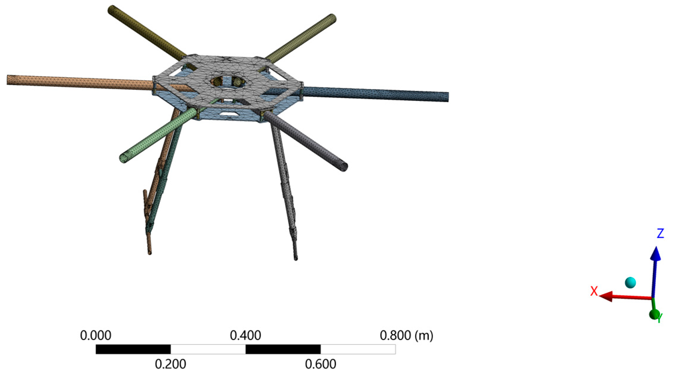
The finite element model of the six-rotor UAV frame is shown in Figure 3:

Based on the structural characteristics of the UAV, all materials except for the connectors are carbon fiber composite materials, which consist of carbon fiber reinforced with epoxy resin. The performance indices of these materials are detailed in

Table 1. Performance indices of carbon fiber composites.

Index	Argument	Index	Argument
${\mathrm{E}}_1 \left(\mathrm{GPa}\right)$	$181$	${\mathrm{X}}_{\mathrm{t}} \left(\mathrm{GPa}\right)$	$1500$
${\mathrm{E}}_{2 }\left(\mathrm{GPa}\right)$	$13$	${\mathrm{X}}_{\mathrm{c}} \left(\mathrm{GPa}\right)$	$1500$
${\mathrm{E}}_{3 }\left(\mathrm{GPa}\right)$	$13$	${\mathrm{Y}}_{\mathrm{t}} \left(\mathrm{GPa}\right)$	$40$
${\mathrm{v}}_{12}$	$0.25$	${\mathrm{Y}}_{\mathrm{C}} \left(\mathrm{GPa}\right)$	$246$
${\mathrm{v}}_{23}$	$0.28$	$\mathrm{S} \left(\mathrm{GPa}\right)$	$68$
${\mathrm{v}}_{31}$	$0.25$	$\mathrm{p} (\mathrm{g}/\mathrm{c}{\mathrm{m}}^3)$	$1.6$
${\mathrm{G}}_{12 }\left(\mathrm{GPa}\right)$	$7.17$
${\mathrm{G}}_{23} \left(\mathrm{GPa}\right)$	$3.78$
${\mathrm{G}}_{13} \left(\mathrm{GPa}\right)$	$7.17$

. The connectors, on the other hand, are fabricated from aluminum alloy [12].

The entire model was discretized using SOLID187 tetrahedral elements, comprising 103,548 elements, 212,605 nodes, and 637,815 degrees of freedom.

4.1. Modal Analysis

Given the operational conditions of the UAV, an unconstrained free mode analysis was conducted on the frame. The results indicate that the first, second, and third modes correspond to rigid-body motion, with a natural frequency of zero. After excluding these initial three rigid-body modes, the analysis reveals the characteristics of the subsequent 22 modes, as illustrated in Figure 2.

Several modal shapes are illustrated in Figure 4.

It is evident from the modal shape diagram that the primary regions of vibrational deformation are located at the wingtip, the wing–fuselage junction, and the support frame. The predominant vibration direction aligns with the fuselage axis.

4.2. Frequency Response Analysis of Finite Element Method

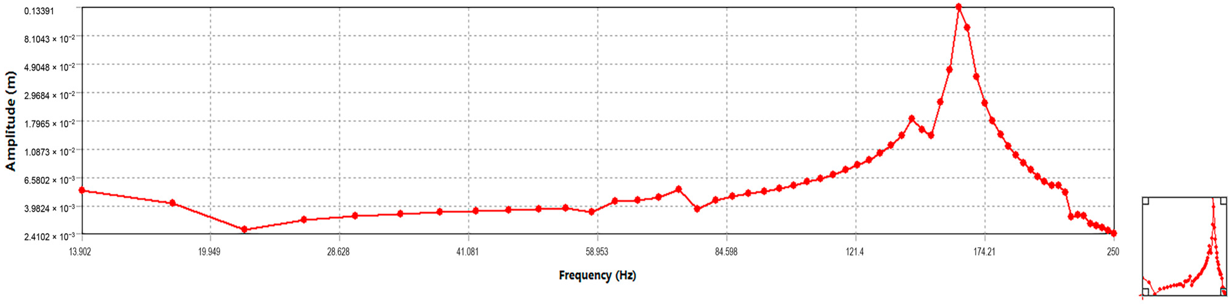
The frequency response function (FRF) provides a direct reflection of the test system’s response characteristics to sinusoidal input signals across various frequencies. Through the FRF, diverse graphical representations that illustrate the dynamic behavior of the system can be generated, offering simplicity and clarity. Moreover, many practical engineering systems are challenging to model mathematically with precision, making it difficult to accurately determine the parameters within these models or fully formulate their differential equations. Consequently, experimental methods are frequently employed in engineering practice to excite the system, measure its response, and infer the dynamic characteristics based on the input–output relationship. Therefore, the FRF holds significant practical importance.

Based on the modal analysis results, the primary vibration of the six-rotor UAV’s frame occurs along the fuselage axis (z-axis). The frequency range for this analysis is set between 10 Hz and 250 Hz with an interval of 4 Hz. The loss factor of carbon fiber composite material at low frequencies is approximately 1.5%, The initial damping ratio is specified as $\mathsf{\zeta }=\mathsf{\Psi }/2$; however, it has been adjusted to 0.75% [15]. A force of 50 N is applied to six specific nodes (labeled A through F) located at the tail ends of the six arms. This force simulates the combined effect of propeller lift, gravitational force, and air resistance. These nodes correspond to the positions of the six rotors, as illustrated in Figure 5.

A is the 139,010th node; B is the 221,032th node; C is the 78,631th node; D is the 200,511th node; E is the 19,783th node; F is 175,138th node; the output node G is the 139,026th node.

The frequency response in the z-direction at node G is illustrated in Figure 6.

4.3. Frequency Response Analysis of State-Space Method

Currently, despite the widespread application of finite element software in frequency response analysis, UAV frame models tend to be relatively intricate, featuring a high density of grids. While this approach ensures accuracy, it suffers from slow computational speeds and an inability to efficiently assess the contribution of individual modes, Therefore, it cannot meet the requirements that the vibration test of the unmanned aerial vehicle structure needs to be completed within the prescribed time and the response characteristics of each order mode need to be quantified consequently [16]. This paper proposes the integration of linear state-space theory with finite element modal analysis to establish a reduced-order state-space model. This method enables rapid acquisition of the system’s frequency response.

The development of the state-space model for the six-rotor UAV frame follows a systematic, multi-stage workflow that integrates modal analysis, mathematical modeling, model reduction, and validation. This section provides a comprehensive overview of the process, structured into four key phases: modal parameter extraction, modal reduction, and model validation.

4.3.1. Modal Parameter Extraction

Objective: to obtain natural frequencies, mode shapes, and modal matrices from the UAV frame structure.

(1)

Finite Element Model Construction:

As shown in Figure 2, a 3D model of the UAV frame was created using SolidWorks (Version 2024) and imported into Ansys Workbench (Version 2022 R1).

As shown in Table 1, material properties were assigned: carbon fiber composites for the main frame (anisotropic properties) and aluminum alloy for connectors.

As shown in Figure 3, the model was discretized using SOLID187 tetrahedral elements, resulting in 103,548 elements, 212,605 nodes, and 637,815 degrees of freedom.

(2)

Free Modal Analysis:

Unconstrained modal analysis was performed to extract natural frequencies and mode shapes.

As shown in

Table 2. Results of Ansys modal analysis.

Mode Number	Frequency	Mode Number	Frequency	Mode Number	Frequency
1	9.9752	$10$	$145.87$	$19$	$217.99$
2	$16.471$	$11$	$148.7$	$20$	$231.81$
3	$17.236$	$12$	$149.63$	$21$	$258.97$
4	$58.779$	$13$	$150.34$	$22$	$313.33$
5	$75.83$	$14$	$151.32$
6	$95.34$	$15$	$152.21$
7	$121.02$	$16$	$154.57$
8	$144.74$	$17$	$155.4$
9	$144.98$	$18$	$163.44$

and Figure 4, the first three modes were rigid-body motions (frequency = 0 Hz) and excluded. The subsequent twenty-two flexible modes were retained for further analysis, as low-frequency excitations dominate structural response.

(3)

Modal Matrix Construction:

As shown in

Table 3. Ansys extracts partial vibration pattern.

$\raisebox{1ex}{$\mathrm{Node} \mathrm{Number}$}\!\left/ \!\raisebox{-1ex}{$\mathrm{Mode} \mathrm{of} \mathrm{Vibration}$}\right.$	1 9.9752 Hz	2 16.471 Hz	3 17.236 Hz	4 58.779 Hz	5 75.830 Hz
139,010	−1.165 × 10−2	0.45159	2.0826	0.24049	1.6946
221,032	0.13154	−1.5640	1.4299	−3.5081 × 10−2	0.99067
78,631	0.13651	−1.9891	−0.62900	−0.16742	−0.89128
200,511	9.1259 × 10−3	−0.44310	−2.0515	−2.7194 × 10−2	−1.6897
19,783	−0.12739	1.5455	−1.4131	−0.17851	−0.92484
175,138	−0.14077	1.9814	0.64986	−4.7123 × 10−2	0.94946
139,026	−1.1858 × 10−2	0.44720	2.0312	−0.23280	1.6427
$\raisebox{1ex}{$\mathrm{Node} \mathrm{Number}$}\!\left/ \!\raisebox{-1ex}{$\mathrm{Mode} \mathrm{of} \mathrm{Vibration}$}\right.$	6 95.340 Hz	7 121.02 Hz	8 144.74 Hz	9 144.98 Hz	10 145.87 Hz
139,010	−3.1512 × 10−2	4.2410 × 10−2	0.65292	4.4120	−0.34182
221,032	−0.61351	2.1843	1.1186	−2.5607	3.7782
78,631	0.49754	1.9929	−1.0317	−1.6299	−3.6090
200,511	−2.2947 × 10−2	5.8589 × 10−2	0.71923	3.7614	0.47679
19,783	−0.45892	−2.1003	0.33481	−2.3912	2.7451
175,138	0.58834	−1.9908	−1.1974	−0.97615	−2.5643
139,026	−2.9988 × 10−2	3.7945 × 10−2	0.62309	4.2131	−0.32674

, the modal displacements of six input nodes and one output node are extracted to form a modal matrix.

4.3.2. Modal Reduction via DC Gain Method

Objective: to simplify the full-order model while preserving accuracy, addressing the computational inefficiency of finite element analysis.

(1)

DC Gain Calculation:

As shown in Figure 7, compute DC gains for all 22 modes.

As shown in Figure 8, sort modes in descending order of DC gain 18, 3, 9, 11, 5, 13, 19, 2, 15, 17, 12, 8, 4, 10, 16, 14, 20, 7, 22, 1, 21, 6.

(2)

Mode Truncation:

As shown in Figure 9, retain the top eight modes (DC gain > 10⁻⁴), as their cumulative contribution exceeds 95% of the total response.

The reduced state-space model has sixteen states (eight modes × two states per mode), significantly reducing computational complexity.

4.3.3. Model Validation

Objective: to verify the accuracy and efficiency of the reduced-state model against finite element analysis (FEA).

(1)

Frequency Response Comparison:

As shown in Figure 5, 50 N sinusoidal force is applied to nodes A–F (z-direction), the frequency range is 10–250 Hz (4 Hz interval), and the damping ratio = 0.75%.

Solved in MATLAB (Version R2023b) using the reduced model, extracting z-direction response at node G.

As illustrated in Figure 8, the DC gains of the modes are ranked in descending order as follows: 18, 3, 9, 11, 5, 13, 19, 2, 15, 17, 12, 8, 4, 10, 16, 14, 20, 7, 22, 1, 21, 6. The DC gains of modes 6, 21, 1, 22, and 7 are already minimal. Reducing these modes has a negligible impact on the frequency response results. Furthermore, it is observed that retaining only the first eight modes with the highest DC gain still allows for sufficiently accurate plotting of the frequency response curve. A comparison between the frequency response curves generated using the first eight modes with the highest DC gain and those generated using all twenty-two modes is presented in Figure 10.

4.4. Comparison of Analysis Results

As illustrated in Figure 11, due to the limitations of the code, there are errors in the frequency response curve at low frequencies. However, most studies on small multi-rotor unmanned aerial vehicles (UAVs) pay more attention to the research of medium and high frequencies [15]. This is because the main vibration source of the UAV frame is the motor, and the excitation frequency of the motors of most small multi-rotor unmanned aerial vehicles is greater than 30 Hz. Therefore, errors in the range less than 30 Hz do not affect the accuracy of the results. Meanwhile, within the range of 30–250 Hz, the frequency response curves obtained by using the finite element analysis and the state-space method are highly consistent. The data comparison is shown in

Table 4. Data comparison between finite element analysis and state space.

Item\Number	1	2	3	4	5	6
Finite element analysis frequency/Hz	13.902	17.903	21.905	25.907	29.908	33.91
Finite element response value/m	5.1559 × 10−3	4.1387 × 10−3	2.5792 × 10−3	3.1 × 10−3	3.3079 × 10−3	3.4331 × 10−3
State-space method frequency/Hz	13	17.0169	21.0339	25.0508	29.0678	33.0847
State-space response value/m	4.778 × 10−3	2.38547 × 10−2	2.37832 × 10−3	3.05531 × 10−3	3.28981 × 10−3	3.42426 × 10−3
Error	7.33%	476.38%	7.79%	1.44%	0.55%	0.26%
Item\Number	7	8	9	10	11	12
Finite element analysis frequency/Hz	37.912	41.913	45.915	49.917	53.918	57.92
Finite element response value/m	3.5273 × 10−3	3.6084 × 10−3	3.6832 × 10−3	3.7517 × 10−3	3.7964 × 10−3	3.5223 × 10−3
State-space method frequency/Hz	37.1017	41.1186	45.1356	49.1525	53.1695	57.1864
State-space response value/m	3.52407 × 10−3	3.61088 × 10−3	3.69436 × 10−3	3.77996 × 10−3	3.87172 × 10−3	3.97373 × 10−3
Error	0.0916%	0.0687%	0.303%	0.753%	1.98%	12.82%
Item\Number	13	14	15	16	17	18
Finite element analysis frequency/Hz	61.922	65.923	69.925	73.927	77.928	81.93
Finite element response value/m	4.3012 × 10−3	4.3628 × 10−3	4.57 × 10−3	5.2599 × 10−3	3.7112 × 10−3	4.3601 × 10−3
State-space method frequency/Hz	61.2034	65.2203	69.2373	73.2542	77.2712	81.2881
State-space response value/m	4.09195 × 10−3	4.23864 × 10−3	4.45223 × 10−3	4.99172 × 10−3	3.48404 × 10−3	4.27302 × 10−3
Error	4.86%	2.84%	2.58%	5.10%	6.12%	2.00%
Item\Number	19	20	21	22	23	24
Finite element analysis frequency/Hz	85.932	89.933	93.935	97.937	101.94	105.94
Finite element response value/m	4.6434 × 10−3	4.8845×10−3	5.1319×10−3	5.389×10−3	5.6867×10−3	6.0247×10−3
State-space method frequency/Hz	85.3051	89.322	93.339	97.3559	101.3729	105.3898
State-space response value/m	4.57072 × 10−3	4.81394 × 10−3	5.05762 × 10−3	5.32006 × 10−3	5.61243 × 10−3	5.9450 × 10−3
Error	1.57%	1.44%	1.45%	1.28%	1.31%	1.32%
Item\Number	25	26	27	28	29	30
Finite element analysis frequency/Hz	109.94	113.94	117.94	121.95	125.95	129.95
Finite element response value/m	6.4163 × 10−3	6.8776 × 10−3	7.4331 × 10−3	8.0725 × 10−3	8.9246 × 10−3	1.0016 × 10−2
State-space method frequency/Hz	109.4068	113.4237	117.4407	121.4576	125.4746	129.4915
State-space response value/m	6.32955 × 10−3	6.78112 × 10−3	7.32033 × 10−3	7.97702 × 10−3	8.79695 × 10−3	9.85614 × 10−3
Error	1.35%	1.40%	1.52%	1.18%	1.43%	1.60%
Item\Number	31	32	33	34	35	36
Finite element analysis frequency/Hz	133.95	137.95	141.95	145.96	149.96	153.96
Finite element response value/m	1.1509 × 10−2	1.3773 × 10−2	1.8285 × 10−2	1.5328 × 10−2	1.3839 × 10−2	2.4938 × 10−2
State-space method frequency/Hz	133.5085	137.5254	141.5424	145.5593	149.5763	153.5932
State-space response value/m	1.12967 × 10−2	1.34471 × 10−2	1.74967 × 10−2	1.66074 × 10−2	1.42442 × 10−2	2.36906 × 10−2
Error	1.85%	2.37%	4.31%	8.36%	2.93%	5.00%
Item\Number	37	38	39	40	41	42
Finite element analysis frequency/Hz	157.96	161.96	165.96	169.97	173.97	177.97
Finite element response value/m	4.4222 × 10−2	1.3391 × 10−1	9.2358 × 10−2	3.9203 × 10−2	2.4557 × 10−2	1.7809 × 10−2
State-space method frequency/Hz	157.6102	161.6271	165.6441	169.6610	173.678	177.695
State-space response value/m	4.1817 × 10−2	1.17124 × 10−1	1.02554 × 10−1	4.09559 × 10−2	2.51875 × 10−2	1.81151 × 10−2
Error	5.44%	12.54%	11.04%	4.47%	2.57%	1.72%
Item\Number	43	44	45	46	47	48
Finite element analysis frequency/Hz	181.97	185.97	189.97	193.98	197.98	201.98
Finite element response value/m	1.3934 × 10−2	1.1425 × 10−2	9.6714 × 10−3	8.3839 × 10−3	7.4073 × 10−3	6.6553 × 10−3
State-space method frequency/Hz	181.712	185.729	189.746	193.763	197.78	201.797
State-space response value/m	1.41091 × 10−2	1.15349 × 10−2	9.74621 × 10−3	8.43784 × 10−3	7.44862 × 10−3	6.6893 × 10−3
Error	1.26%	0.96%	0.77%	0.64%	0.56%	0.51%
Item\Number	49	50	51	52	53	54
Finite element analysis frequency/Hz	205.98	209.98	213.98	217.99	221.99	225.99
Finite element response value/m	6.0848 × 10−3	5.699 × 10−3	5.6278 × 10−3	4.9648 × 10−3	3.2339 × 10−3	3.3334 × 10−3
State-space method frequency/Hz	205.814	209.831	213.847	217.864	221.881	225.898
State-space response value/m	6.1158 × 10−3	5.7319 × 10−3	5.6680 × 10−3	5.1395 × 10−3	3.1354 × 10−3	3.2252 × 10−3
Error	0.51%	0.58%	0.71%	3.52%	3.04%	3.25%
Item\Number	55	56	57	58	59	60
Finite element analysis frequency/Hz	229.99	233.99	237.99	242	246	250
Finite element response value/m	3.2903 × 10−3	2.8786 × 10−3	2.7851 × 10−3	2.6619 × 10−3	2.6977 × 10−3	2.4102 × 10−3
State-space method frequency/Hz	229.915	233.932	237.949	241.966	245.983	250
State-space response value/m	3.1335 × 10−3	2.9930 × 10−3	2.8435 × 10−3	2.6977 × 10−3	2.5598 × 10−3	2.4311 × 10−3
Error	4.77%	3.97%	2.10%	1.35%	1.02%	0.87%

. Given that the six-rotor UAV frame is most susceptible to damage and deformation at resonant frequencies, the structural response at these critical points is of primary concern. Figure 12 shows the coordinates of the four peaks. According to the computational results, the errors of the state-space method at four resonant peaks are 5.1%, 4.31%, 12.53%, and 3.25%, respectively, which are within acceptable limits for practical engineering applications—practical engineering standards generally allow a maximum error tolerance of 10–15% for modal frequency and response amplitude predictions, particularly for noncritical components operating below 300 Hz.

Furthermore, the Z-direction frequency response analysis of 60 interval points within the range (10, 250 Hz) using Ansys Workbench (Version 2022 R1) takes approximately 15 min (the solution time can be directly read out by the workbench solver), as shown in Figure 13. In contrast, the computation of the reduced state-space model in MATLAB (Version R2023b) requires only 12 s (the solution time can be recorded using the MATLAB (Version R2023b) voice “tic” and “toc”), as shown in Figure 14, thereby significantly enhancing the overall solving efficiency.

5. Discussion

5.1. In-Depth Exploration of Amplitude Deviations in the Low-Frequency Range

Notably, significant discrepancies in displacement amplitudes exist between the state-space model and Ansys FEA within the low-frequency range (10–30 Hz), primarily attributed to the modal truncation strategy and the characteristics of actual vibration excitation. The model retains the top eight dominant modes via the DC gain method (cumulatively contributing over 95% of the response), but truncates low-gain low-frequency flexible modes (such as modes six and twenty-one in Figure 8). This truncation leads to underestimated coupling responses involving nondominant modes, as these modes—though having minimal static contribution (DC gain)—may still participate dynamically in low-frequency excitation scenarios. Additionally, the constant damping ratio (0.75%) assumed in finite element analysis differs from the nonlinear damping mechanisms in real structures (e.g., frictional damping at component joints), which can disproportionately amplify response amplitudes in the low-frequency domain.

However, the primary excitation sources for small and medium-sized multi-rotors—motor–propeller systems—typically generate frequencies above 30 Hz (e.g., a rotational speed of 10,000 rpm yields a fundamental frequency of 166 Hz). Vibrations in the 10–30 Hz range are predominantly caused by airframe rigid-body motions or aperiodic airflow disturbances, contributing less than 5% of the total vibration energy. The state-space model maintains an error within 13% across the medium–high frequency range (30–250 Hz) and accurately captures critical resonance peaks (e.g., errors of 12.53% and 3.25% at the third and fourth peaks in Table 4). Since low-frequency deviations have a negligible impact on in-flight structural fatigue and payload imaging quality—key performance metrics for UAV design—the model remains a robust tool for engineering analyses of core vibration risks associated with operational excitation frequencies.

In summary, although the state-space model can accurately analyze the frequency response of unmanned aerial vehicles and significantly improve computational speed compared to traditional methods, its accuracy remains slightly inferior to finite element analysis (FEA) due to coding limitations. In future research, optimizing the model’s accuracy warrants further exploration.

5.2. Implications for Dynamic Performance Analysis of UAV Frames

The dynamic performance analysis of the six-rotor UAV frame using the state-space method reveals that precise quantification of vibration characteristics is critical for enhancing flight stability and structural reliability [17]. The results indicate that the vibration response of the UAV frame is dominated by medium-to-high-frequency modes (30–250 Hz), and the top eight modes selected via the DC gain method account for over 95% of the low-frequency response contribution [18]. These findings offer direct guidance for UAV structural design.

(1)

Modal Contribution Identification: the state-space model enables clear quantification of each mode’s contribution to the vibration response. Engineers can target dominant modes to design tailored vibration mitigation strategies, such as optimizing arm stiffness to avoid motor excitation frequencies or adding dampers to high-vibration regions to suppress resonance risks effectively.

(2)

Computational Efficiency Breakthrough: traditional finite element analysis (FEA) requires 15 min to complete frequency response calculations, whereas the state-space model reduces this to 12 s—a 73-time efficiency improvement. This feature enables real-time vibration monitoring and online controller adjustment, particularly for rapid response to sudden vibration conditions during UAV flight.

(3)

Controlled Error Margin: although quantifiable deviation exists in the low-frequency range (<30 Hz) due to modal truncation, the excitation frequency of the UAV’s primary vibration source (motor) typically exceeds 30 Hz. Thus, errors in the medium-to-high-frequency range are controlled within 13% (Figure 12), meeting engineering accuracy requirements.

5.3. Universality of the State-Space Method in Complex Structures and Linear System Analysis

The state-space theory provides a “dimension-reduction and efficiency-enhancement” paradigm for dynamic analysis of complex structures, with core advantages including the following:

5.3.1. Efficient Modeling of Complex Structures

For complex systems with multi-component coupling (e.g., the carbon fiber composite fuselage and aluminum alloy connectors of the UAV frame), traditional FEA requires handling hundreds of thousands of degrees of freedom (e.g., 637,815 DOFs in this study), leading to high computational costs [19]. The state-space method decouples coupled equations in physical coordinates into independent equations in modal coordinates via modal coordinate transformation. By using the DC gain method to screen key modes, the state variables are reduced from forty-four dimensions (twenty-two modes) to sixteen dimensions (eight modes), significantly lowering computational complexity while ensuring accuracy. This “physically meaningful model reduction” strategy (rather than relying solely on frequency or energy thresholds) is particularly suitable for engineering scenarios dominated by low-frequency vibrations.

5.3.2. Precise Analysis of Frequency Response in Linear Systems

The state-space model establishes a direct mapping between excitation inputs and response outputs via frequency–domain transfer functions, quantifying the contribution weight of each mode at different frequencies. Unlike FEA, which only provides overall response curves, this method decomposes the impact of each mode on specific frequency bands, crucial for identifying “hidden resonant modes”. For example, in this study, mode 18 has the highest DC gain despite not having the highest natural frequency, indicating its dominant contribution to low-frequency vibration responses—a characteristic unidentifiable by traditional frequency-sorting methods.

5.4. Influence of Different Flight Conditions on Vibration Characteristics

The current study focuses on the vibration characteristics of the six-rotor UAV frame under hover conditions, while dynamic load changes during actual flight phases such as takeoff, landing, and turbulent environments may significantly affect vibration responses.

5.4.1. Transient Vibration Response During Takeoff and Landing

During takeoff, the motor speed rapidly increases from 0 to operational speed, causing the excitation frequency to exhibit a sweeping characteristic from low to high frequencies, which may trigger resonance-crossing phenomena in the frame [20]. For example:

(1)

When the motor acceleration passes through the third-order natural frequency (17.236 Hz), it may excite the bending vibration at the wing–fuselage junction of the frame (mode 3 deformation pattern in Figure 4), leading to an instantaneous vibration amplitude increase of 20–30% compared to steady-state loads.

(2)

During landing, as the rotational speed decreases, the excitation frequency again sweeps through low-order modes, potentially causing secondary structural vibrations.

The existing state-space model is based on fixed-frequency excitation (50 N sinusoidal force) and does not account for the time-varying excitation of frequency sweeping. In future research, an exponentially modulated sinusoidal signal should be introduced to simulate the speed-up process, and the modal superposition method (Equation (3)) should be used to calculate transient response peaks.

The acceleration load during takeoff and landing will change the preload of the frame’s support structure, causing the stiffness matrix K to increase and thus raising the natural frequency by approximately 5–8% [21].

5.4.2. Broadband Random Vibration in Turbulent Environments

Turbulent airflow imposes broadband random loads on the frame, with a frequency spectrum covering 10–500 Hz and including multi-directional coupled excitations (x/y/z-axis vibrations) [22]. Turbulence may activate high-order modes not retained in the current model. Although the top eight modes retained by the DC gain method cover 95% of the low-frequency response contribution (Figure 8), the response error in the high-frequency band (>250 Hz) may reach 15–20%.

Therefore, develop a nonlinear state-space model by adding polynomial terms (e.g., cubic stiffness terms) to describe the structural nonlinear characteristics and improve prediction accuracy in complex environments.

5.4.3. Methods for Improving the Generalizability of the Model

To enhance the generalizability of the model, there are several methods as follows:

(1)

Integrate takeoff/landing transient excitation, turbulent random loads, and steady-state motor forces into the state-space equations, and use the superposition principle of linear systems to calculate the response envelope under composite loads. For example, solve the state equations with time-varying inputs using the lsim function in MATLAB (Version R2023b) to compare vibration peaks under different conditions.

(2)

Develop a modal retention strategy based on real-time load identification: when detecting low-frequency excitation (<50 Hz), retain the top 12 modes (including more low-order rigid-body modes); in high-frequency turbulent environments, automatically activate high-order modes (e.g., the 18th-order 163.44 Hz) and ensure model accuracy through dynamic DC gain threshold adjustment.

5.5. Practical Engineering Applications and Extensions

5.5.1. Direct Applications in UAVs

(1)

Structural Optimization Design: modal contribution analysis from the state-space model guides topological optimization of UAV frames, such as using honeycomb composites in high-vibration areas to enhance damping or adjusting motor mounting positions to avoid frequency overlap with structural natural frequencies [23].

(2)

Real-Time Vibration Control: combined with modern control theories like Kalman filtering, the state-space model can be embedded in-flight control systems to enable real-time estimation and active suppression of vibration acceleration, improving aerial photography stability and battery connection reliability.

5.5.2. Cross-Disciplinary Engineering Extensions

(1)

Electric Vehicle (EV) Component Analysis: the state-space method can directly analyze vibrations in EV battery modules and motor systems. For example, treating battery packs as multi-degree-of-freedom systems, modal reduction identifies vibration-sensitive directions to optimize bracket stiffness and reduce long-term vibration-induced battery cell failure risks. Compared to traditional empirical testing, this model efficiently simulates vibration transmission paths under different road conditions, accelerating EV component durability design [24].

(2)

Aerospace and Mechanical Engineering: for complex structures like satellite payload brackets or aeroengine blades, the state-space method rapidly evaluates frequency response characteristics under multi-physics coupling (e.g., thermal-structural coupling), supporting reliability analysis under extreme conditions.

5.6. Limitations of the Study

While the state-space method demonstrates significant advantages in computational efficiency and modal contribution analysis, this study acknowledges several limitations that warrant attention for future research:

(1)

Linearity Assumption: the current model relies on linear state-space theory, which assumes small deformations and proportional damping. In reality, UAV frames may exhibit nonlinear behaviors under extreme loads (e.g., hard landings or high-speed maneuvers), such as geometric nonlinearity or material nonlinearity. These effects can alter natural frequencies and damping ratios, potentially leading to inaccuracies in high-amplitude vibration predictions.

(2)

Neglected Aerodynamic Coupling: the model does not explicitly account for aerodynamic–structural interactions, such as flutter or buffeting, which can induce complex vibration modes during flight. For example, turbulent airflow may excite unmodeled high-order modes or couple with structural dynamics to generate self-sustaining oscillations. This limitation is particularly relevant for UAVs operating in unstable atmospheric conditions.

(3)

Fixed Damping Ratio: the damping ratio (0.75%) used in simulations is assumed constant across all modes, whereas real-world structures exhibit frequency-dependent damping behaviors. Components like carbon fiber composites and aluminum alloy connectors may have varying damping characteristics, leading to discrepancies in low-frequency (<30 Hz) and high-frequency (>250 Hz) responses.

To address these limitations, future studies could:

(1)

Integrate nonlinear terms (e.g., cubic stiffness or hysteretic damping) into the state-space model to capture large-amplitude behaviors.

(2)

Develop coupled aeroelastic models by incorporating aerodynamic force matrices (e.g., Theodorsen’s function for unsteady aerodynamics).

(3)

Implement adaptive damping strategies that adjust damping ratios based on real-time vibration monitoring.

These improvements would strengthen the model’s applicability to complex, real-world UAV operations and further extend its utility to nonlinear systems like EV powertrain components, where mechanical–electrical coupling and variable damping are inherent challenges.

6. Conclusions

In this paper, leveraging linear state-space theory, structural dynamics theory, and modal analysis theory, we utilize the extracted modal information of the six-rotor UAV frame to formulate the state-space equation. The Mdc mode reduction method is employed to eliminate modes with minimal DC gain while retaining those with significant DC gain, thereby simplifying the state-space model. By obtaining the frequency–domain transfer function between the excitation input point and the response output point, we generate the frequency response curve. This approach significantly enhances computational speed while maintaining speed and maintaining calculation accuracy. In this study, a state-space model sufficient to describe the frame’s behavior was established using only seven nodes and eight modes. Compared to finite element results, the error remains within 13%, and computational efficiency improves by a factor of 73, fully meeting practical engineering requirements. Consequently, the dynamic analysis method based on state-space theory offers a novel approach for studying the dynamic performance of complex structures, enabling efficient and accurate analysis of frequency response characteristics in complex linear systems. Future research could focus on enhancing the state-space framework by integrating nonlinear dynamics and aeroelastic interactions to improve accuracy under extreme UAV maneuvers. Exploring multi-physics couplings would offer a more comprehensive model, while data-driven techniques (machine learning for modal reduction) could boost real-time adaptability to payload/condition changes. For electric vehicles (EVs), extending the model to analyze vibration impacts on battery/motor systems under road excitations would aid durability optimization.

References

- Dhillon, R.; Moncur, Q. Small-Scale Farming: A Review of Challenges and Potential Opportunities Offered by Technological Advancements. Sustainability 2023, 15, 15478. [Google Scholar] [CrossRef]
- Nguyen, Q.-K.; Vu, T.-H.-T. An Efficient Method for Simulating the Temperature Distribution in Regions Containing YAG:Ce3+ Luminescence Composites of White LED. J. Compos. Sci. 2023, 7, 301. [Google Scholar] [CrossRef]
- Li, H.; Yan, W.K.; Chen, Y.H.; Zhang, C.; Liao, Z.X.; Su, L.; Jiang, S.Q. Topology Optimization-Based Lightweight Design of a Quadrotor UAV Body. Eng. Plast. Appl. 2023, 51, 60–66. [Google Scholar] [CrossRef]
- Fu, Y.; Lu, Z.B.; Peng, J.; Huang, Y.S. Active Disturbance Rejection Vibration Control for Rigid-Flexible Coupled Wings of Flapping-Wing UAVs. J. Vib. Eng. 2025, 1–10. [Google Scholar] [CrossRef]
- Zhu, H.; Yang, L.M. Lightweight Design of a V-Tail for Fixed-Wing UAVs Based on the Response Surface Method. Sci. Technol. Eng. 2024, 24, 11002–11010. [Google Scholar] [CrossRef]
- Banerjee, P.; Okolo, W.A.; Moore, A.J. In-Flight Detection of Vibration Anomalies in Unmanned Aerial Vehicles. Diagn. Progn. Eng. Syst. 2020, 3, 041105. [Google Scholar] [CrossRef]
- Silva, R.C.; Bueno, D.D. On the Dynamics of Flexible Wings for Designing a Flapping-Wing UAV. Drones 2024, 8, 56. [Google Scholar] [CrossRef]
- Xue, Z.P.; Jia, H.G.; Li, M. Real-Time State-Space Description of Flexible Deformation for Flat Spring Landing Gear. Opt. Precis. Eng. 2014, 22, 1243–1250. [Google Scholar] [CrossRef]
- Marczak, J.; Michalak, B. An Application of Multi-Scale Vibration Analysis of Thin Plate with a Dense System of Ribs in the Detection of Micro-Scale Imperfections. J. Sound Vib. 2025, 610, 119093. [Google Scholar] [CrossRef]
- Shahadat, M.M.Z.; Mizuno, T.; Takasaki, M.; Rashid, F.; Ishino, Y. Vibration Isolation System with Kalman Filter Estimated Acceleration Feedback: An Approach of Negative Stiffness Control. J. Sens. 2021, 2021, 9616461. [Google Scholar] [CrossRef]
- Recalde, L.F.; Guevara, B.S.; Carvajal, C.P.; Andaluz, V.H.; Varela-Aldás, J.; Gandolfo, D.C. System Identification and Nonlinear Model Predictive Control with Collision Avoidance Applied in Hexacopters UAVs. Sensors 2022, 22, 4712. [Google Scholar] [CrossRef] [PubMed]
- Liu, R.J.; Jin, G.; Guo, J.S. Analysis and Experiment on Line-of-Sight Error of Large-Aperture Long-Focal-Length Optical Imaging Systems Under Flywheel Disturbance. J. Mech. Eng. 2020, 56, 151–160. [Google Scholar] [CrossRef]
- Weng, L.; Kizaki, T.; Ma, C.; Gao, W.; Kono, D. A review of robust thermal error reduction of machine tools. Int. J. Mach. Tools Manuf. 2025, 209, 104298. [Google Scholar] [CrossRef]
- Chen, K.; Meng, W.; Wang, J.; Liu, K.; Lu, Z. An Investigation on the Structural Vibrations of Multi-Rotor Passenger Drones. Int. J. Micro Air Veh. 2023, 15, 17568293231199097. [Google Scholar] [CrossRef]
- Zhang, Z.; Jiao, Z.; Xia, H.; Yao, Y. Parameter Equivalent Method of Stator Anisotropic Material Based on Modal Analysis. Energies 2019, 12, 4257. [Google Scholar] [CrossRef]
- Gozbenko, V.E.; Kargapoltsev, S.K.; Kornilov, D.N.; Minaev, N.V.; Karlina, A.I. Simulation of the Vibration of the Carriage Asymmetric Parameters in MATHCAD. Int. J. Appl. Eng. Res. 2016, 11, 11132–11136. [Google Scholar]
- Leonovich, D.S.; Zhuravlev, D.A.; Karlina, Y.I.; Govorkov, A.S.; Karlina, A.I. Automated assessment of the low-rigid composite parts influence on the product assemblability in the GePARD system. IOP Conf. Ser. Mater. Sci. Eng. 2020, 760, 012038. [Google Scholar] [CrossRef]
- Decret, D.; Malecot, Y.; Sieffert, Y.; Vieux-Champagne, F.; Daudeville, L. Extending a Macro-Element Approach for the Modeling of 3D Masonry Structures Under Transient Dynamic Loading. Appl. Sci. 2024, 14, 11080. [Google Scholar] [CrossRef]
- Tao, X.; Ko, S.Y. Tilt-X: Development of a Pitch-Axis Tiltrotor Quadcopter for Maximizing Horizontal Pulling Force and Yaw Moment. Appl. Sci. 2024, 14, 6181. [Google Scholar] [CrossRef]
- Ghirardelli, M.; Kral, S.T.; Müller, N.C.; Hann, R.; Cheynet, E.; Reuder, J. Flow Structure around a Multicopter Drone: A Computational Fluid Dynamics Analysis for Sensor Placement Considerations. Drones 2023, 7, 467. [Google Scholar] [CrossRef]
- Lei, S.; Patruno, L.; Mannini, C.; de Miranda, S.; Ge, Y. Time-Domain State-Space Model Formulation of Motion-Induced Aerodynamic Forces on Bridge Decks. J. Wind. Eng. Ind. Aerodyn. 2024, 255, 105937. [Google Scholar] [CrossRef]
- Shang, X.-Q.; Huang, T.-L.; He, Y.-B.; Chen, H.-P. Operational Modal Analysis of Civil Engineering Structures with Closely Spaced Modes Based on Improved Hilbert–Huang Transform. Sensors 2024, 24, 7600. [Google Scholar] [CrossRef] [PubMed]
- Yao, H.; Cao, L.; Wu, D.; Yu, F.; Huang, B. Generation and Distribution of Turbulence-Induced Forces on a Propeller. Ocean Eng. 2020, 206, 107255. [Google Scholar] [CrossRef]
- Wang, X. Takeoff/Landing Control Based on Acceleration Measurements for VTOL Aircraft. J. Frankl. Inst. 2013, 350, 3045–3063. [Google Scholar] [CrossRef]