Research on Model Identification of Permanent Magnet DC Brushless Motor Based on Auxiliary Variable Subspace Identification Algorithm

Abstract

This paper proposes a model identification method based on the auxiliary variable closed-loop subspace identification algorithm to address the problem of modeling difficulties caused by various complex factors affecting permanent magnet brushless DC motors in practical working conditions. This method breaks through the limitations caused by the correlation between input signals and noise in traditional subspace identification algorithms. By introducing auxiliary variables, it effectively avoids the projection process, simplifies the complex calculations of principal component analysis, and improves the practicality and efficiency of the algorithm. When constructing a data-driven identification model, the actual situation of measurement data being contaminated by noise has to be fully considered. Orthogonal compensation matrices and auxiliary variables were used to construct uncorrelated terms for noise, thereby eliminating the negative impact of noise on the model’s identification accuracy. The effectiveness of the proposed identification algorithm was verified by collecting data through a chassis dynamometer simulation test of a vehicle-mounted permanent magnet brushless DC motor. The results show that compared with the traditional N4SID algorithm, the proposed closed-loop subspace identification algorithm based on auxiliary variable principal component analysis exhibits higher model identification accuracy, stronger anti-interference ability, and better stability in both noise-free and noise-contaminated conditions, providing a more reliable model basis for motor performance evaluation and control strategy design.

1. Introduction

In many industrial and daily application scenarios today, permanent magnet DC brushless motors are widely used due to their high efficiency, high reliability, and many other advantages. However, in its actual operation, various complex environmental factors inevitably have an impact on the motor system [1,2]. For example, the vibration generated by a motor during operation is a common physical phenomenon. Vibration may originate from various factors such as the mechanical structural imbalance of the motor itself, unstable installation, or the inaccurate meshing of the transmission device [3]. When a motor operates in a vibrating environment, the relative positions and interaction forces between its internal components undergo small but continuous changes, which can introduce system process noise and interfere with the normal operating state of the motor and the accuracy of control signals [4,5,6]. For example, in the case of heating, the motor accumulates heat during its operation due to factors, such as winding current and eddy current losses in the iron core. The increase in temperature can cause changes in the physical properties of motor materials, such as an increase in resistivity, which can affect the electrical performance of the motor and generate noise signals that can be mixed into the system’s process [7,8]. In addition, various factors such as electromagnetic interference, humidity changes, and dust particle intrusion that may exist in the environment can generate system process noise to varying degrees, which has a negative impact on the performance and control accuracy of the motor [9,10].

Given these practical situations, when modeling permanent magnet brushless DC motors, the noise factors that exist in reality must not be ignored [11,12,13]. The key situation of including noise in the model must be fully considered so that the established model can more realistically and accurately reflect the operating characteristics of the motor under actual working conditions [14,15], providing a reliable theoretical basis and data support for subsequent motor performance evaluation and control strategy design, etc., ensuring that the motor can stably, efficiently, and accurately play its role in the application field, meet the high-precision requirements [16,17,18] of industrial production and the needs of people’s daily life for convenience. In addition, in model identification, when the driving data are affected by noise interference, it will have a significant impact on the accuracy of model identification. Measurement noise can mask or distort the true features of measurement data, leading to the inaccurate extraction of useful information from the data and subsequently affecting the accuracy of model parameters. Due to the influence of noise, the model may perform well on training data but cannot make good predictions on new data, resulting in a decrease in the model’s generalization ability. Meanwhile, measuring noise may lead to unstable model identification results, making the model susceptible to external interference in practical applications. Therefore, considering the influence of noise is one of the important aspects to improve the model identification performance [19,20,21].

The current data-driven modeling methods show a diversified trend in motor modeling. Multiple algorithms have been applied [22,23], such as the BP neural network for motor inverse model construction to achieve high-precision position control and deep learning algorithms for the modeling and control of brushless DC motor drive systems. There are also methods such as support vector machine, kernel principal component analysis, extreme learning machine, and the physical information neural network, each with their own characteristics and advantages, used for modeling scenarios of different motors [24,25]. These methods have many advantages, such as improving model accuracy, accurately capturing the complex characteristics and nonlinear relationships of motors, learning, and training effective models based on actual data, adapting these to different types of motors and complex working conditions [26,27], and integrating multi-source data to promote the intelligent development of motor systems, assisting in performance evaluation, fault prediction, and optimized control. However, there are also challenges in current research, such as the poor interpretability of models, high requirements for data quality and quantity, the need to improve generalization ability, and some models are complex and have low computational efficiency.

In the research process of the parameter identification of data-driven motor models, the measurement data used will inevitably be affected by measurement noise [28,29,30]. The main reasons for this are as follows: Firstly, the sensor itself has certain accuracy limitations and cannot measure physical quantities completely accurately, resulting in measurement results containing errors that manifest in the form of noise. Secondly, electromagnetic interference, temperature changes, vibrations, and other factors in the operating environment of the motor can affect the measurement of the sensor, resulting in measurement data deviating from the true value. In addition, the measurement signal may be subject to interference during transmission, resulting in damage to the integrity of the signal and the inclusion of noise in the measurement data [31,32,33]. Finally, when preprocessing and filtering measurement data, improper processing methods may introduce additional errors and exacerbate the impact of measurement noise.

The presence of these measurement noises will have a significant impact on the accuracy of model identification [34]. Measurement noise can mask or distort the true features of measurement data, leading to the inaccurate extraction of useful information from the data and subsequently affecting the accuracy of model parameters. Due to the presence of noise, the estimation of model parameters may deviate, making it difficult for the model to accurately reflect the actual characteristics of the motor [35,36,37]. Meanwhile, due to the influence of noise, the model may perform well on training data but cannot make good predictions on new data, resulting in a decrease in the model’s generalization ability. In addition, measuring noise may lead to unstable estimation results of model parameters, making the model susceptible to external interference in practical applications and reducing its stability. Therefore, in the research of data-driven motor model parameter identification [38,39], effective noise processing methods such as data preprocessing, filtering, denoising, etc., need to be adopted to reduce the impact of measurement noise on the accuracy of model identification and improve the accuracy and reliability of the model.

In the application process of traditional subspace identification algorithms, the correlation between input signals and noise often interferes with the effectiveness of the algorithm. To address this issue, considering the situation where the driving data are contaminated by noise, a permanent magnet DC brushless motor model identification method based on an auxiliary variable closed-loop subspace identification algorithm was studied. This study draws on the model theory based on variable errors and introduces the key element of auxiliary variables [40,41], thus avoiding the complex projection process in classical subspace identification algorithms. At the same time, in the process of conducting principal component analysis on data, it effectively avoids the complex calculations faced when solving the analysis object in the previous principal component analysis process [42,43], greatly improving the practical application value and performance of the algorithm, and providing a more reliable theoretical basis and technical guarantee for related research and practical applications. The research contributions of this paper can be summarized into the following three points:

(1) A model identification method for automotive direct drive motors has been proposed, which can effectively handle the situation of noise pollution in driving data and improve the accuracy and stability of model identification.

(2) Drawing on the model theory based on variable error, auxiliary variables are introduced to avoid the complex projection process in traditional subspace identification algorithms, simplify algorithm implementation, and reduce computational complexity.

(3) The effectiveness and superiority of the proposed algorithm in actual working conditions were verified through the chassis dynamometer simulation testing of the vehicle-mounted permanent magnet DC brushless motor, providing a more reliable model basis for motor performance evaluation and control strategy design.

The rest of this paper is organized as follows. The construction of a data-driven identification model is presented in Section 2. The improved closed-loop subspace identification algorithm for the motor model considering noise pollution is designed in Section 3. The verification and analysis of results are provided in Section 4, followed by the Conclusion in Section 5.

2. Construction of Data-Driven Identification Model

2.1. Mathematical Model of Permanent Magnet DC Brushless Motor

The mechanism model clarifies the causal relationship of variables based on physical laws, while the data-driven model explores complex patterns in actual data. The combination of the two enables the model to reflect on the physical characteristics of the system and correct errors caused by simplified assumptions, thus more accurately describing the dynamic characteristics of the system and adapting to different working and load conditions. In addition, the mechanism model provides the basis for the physical structure and main dynamic characteristics of the system, and the data-driven model optimizes and supplements it on this basis, which helps to reduce the difficulty and workload of identification and improve identification efficiency.

The torque balance equation for the output shaft of a permanent magnet brushless DC motor [44] is as follows:

$$J\dot{\omega }+b\omega =K_{t}i-T_l,$$

(1)

where J is the moment of inertia of the motor rotor; b is the damping coefficient; K_t is the motor torque constant; T_l is the motor load torque; i is the line current; and $\omega$ is the motor speed. The dynamic voltage balance equation of the equivalent circuit of a permanent magnet brushless DC motor is given as follows:

$$U=Ri+L\dot{i}+K_a\omega ,$$

(2)

where $U$ is the line voltage; R is the equivalent line resistance of the winding; L is the equivalent inductance of the winding; and K_a is the back electromotive force coefficient.

Assuming that the state vector x contains the motor current and speed, and given that the input u contains motor voltage $U$ and load torque T_l, and y is the sensor measurement output, the state space equation of the permanent magnet brushless DC motor model can be expressed as follows:

$$\dot{x}=Ax+Bu,$$

(3)

$$y=Cx,$$

(4)

where $x=\left[\begin{array}{c}i\\ \omega \end{array}\right]$, $A=\left[\begin{array}{cc}-{\displaystyle \frac{R}{L}}& -{\displaystyle \frac{K_a}{L}}\\ {\displaystyle \frac{K_t}{J}}& -{\displaystyle \frac{b}{J}}\end{array}\right]$, $B=\left[\begin{array}{cc}{\displaystyle \frac{1}{L}}& 0\\ 0& -{\displaystyle \frac{1}{J}}\end{array}\right]$, $u=\left[\begin{array}{c}U\\ T_l\end{array}\right]$, $C=\left[\begin{array}{cc}1& 0\\ 0& 1\end{array}\right]$.

2.2. Model Identification Data Collection

According to the nameplate parameters of the motor, the mass of the motor is 18.6 kg; the rated power of the motor is 3 Kw; the peak torque of the motor is 150 Nm; and the peak speed of the motor is 750 r/min. In order to obtain the driving data required for the identification of the permanent magnet DC brushless motor model, as shown in Figure 1, a bench characteristic test of the motor was conducted, and multiple sets of data were classified and collected. As shown in the figure, the motor, speed, torque sensor, and magnetic powder brake are fixed on the base with fixtures to ensure consistent horizontal height. The three are connected with coupling to meet their coaxial requirements. A constant voltage source is used to provide stable input voltage for motor characteristic testing, and magnetic powder brakes are used to apply simulated loads. In addition, in order to minimize the disturbance of temperature rise on the test data of motor characteristics, a high-power blower is used to cool the motor, and a flow water cooling device is used to cool the magnetic powder brake.

The motor is directly controlled by a motor controller, and by providing control signal voltages for different controllers, different motor power requirements can be simulated. By using a control signal generator to send different control signals to the motor controller, it is possible to achieve motor control response testing under different power requirements. Torque/speed sensors are used to measure the torque and speed of the driving motor under different control signals, while current sensors and voltage sensors can measure the line current and line voltage of the motor. During actual testing, the control signal voltage is gradually increased according to a fixed step size, allowing for the collection of multiple sets of motor characteristic test datasets under different operating conditions. The actual operating signal of the motor controller is within the range of 1 V to 3 V, and this control signal voltage range corresponds to the range that the motor’s torque can reach. Given different motor control signals, the starting voltage of the motor controller control signal is 1 V, which increases by 0.2 V each time until the signal voltage reaches 3 V. Under the corresponding motor control signal, the motor load is continuously increased, and the torque/speed sensor can measure the torque/speed values under different loads. When the control signal voltage of the motor controller is 3 V, the motor voltage stabilizes at approximately 72 V. When the control signal voltage of the motor controller is 1 V, the motor voltage stabilizes at approximately 54 V. In addition, multiple sets of experimental data need to be collected independently for data-driven model identification and validation. The characteristic relationship between the line voltage, line current, speed, and torque of the motor collected from the motor characteristic test is shown in Figure 2.

2.3. Model Identification Considering the Noise Pollution of Driven Data

To achieve model identification, the motor model in Equations (3) and (4) is represented as a discrete-time linear time-invariant system in the following form:

$$\left\{\begin{array}{l}x(k+1)=Ax(k)+B{u}_n(k)+\epsilon (k)U\hfill \\ y_n(k)=Cx(k)+D{u}_n(k)\hfill \end{array}\right.,$$

(5)

where $x(k)\in R^n$ represents the system state value of the noise-pollution-free model; $u_n(k)\in R^l$ represents the system input value of the noise-pollution-free model; $y_n(k)\in R^m$ represents the system measurement value of the noise-pollution-free model; and $\epsilon (k)\in R^n$ represents the system’s process noise term.

In the construction of the noise pollution model (NPM), considering the situation where the measurement data used for data-driven model identification are contaminated by noise, the measurement input data and measurement output data used in the identification process can be represented as follows:

$$\left\{\begin{array}{l}u(k)=u_n(k)+w(k)\\ y(k)=y_n(k)+v(k)\end{array}\right.,$$

(6)

where $w(k)\in R^l$ is the input measurement noise and $v(k)\in R^m$ is the output measurement noise. The process noise $\epsilon (k)$; input measurement noise $w(k)$; and output measurement noise $v(k)$ are all white noise and are not directly related to the system inputs $u_n(k)$ in the noise-pollution-free model at past times.

If the current moment is defined as time point k, then the past and future input data matrices [45] can be represented as follows:

$$y_p(k)=\left[\begin{array}{c}y(k-p)\\ y(k-p+1)\\ ⋮\\ y(k-1)\end{array}\right]\in R^{mp},$$

(7)

$$y_f(k)=\left[\begin{array}{c}y(k)\\ y(k+1)\\ ⋮\\ y(k+f-1)\end{array}\right]\in R^{mf}.$$

(8)

In the formula, subscripts p and f not only distinguish between past and future moments but also represent the number of vectors in the past and future, which are numerical values. The definitions of vectors $w_f(k)\in R^{lf}$, $w_f(k)\in R^{lf}$, and ${\epsilon }_f(k)\in R^{nf}$ are similar to that of $y_f(k)$.

The Hankel matrices for past output and future output are as follows:

$$Y_p=\left[y_p(k),y_p(k+1),\dots ,y_p(k+N-1)\right]\in R^{mp\times N},$$

(9)

$$Y_f=\left[y_f(k),y_f(k+1),\dots ,y_f(k+N-1)\right]\in R^{mf\times N}.$$

(10)

Arranging $y(k)$ and $y(k+1)$ to $y(k+f-1)$ in columns yields a new matrix equation as shown below:

$$y_f(k)={\Gamma }_{f}x(k)+H_f{u}_f(k)-H_f{w}_f(k)+G_f{\epsilon }_f(k)+v_f(k),$$

(11)

The generalized observable matrix and the lower triangular block Toeplitz matrix in the equation are defined in the same way as the classical subspace algorithm. Then, the vector ${\xi }_f(k)=\left[\begin{array}{c}{y}_f(k)\\ u_f(k)\end{array}\right]\in R^{(lf+mf)}$ is defined and substituted into Equation (11) as follows:

$$\left[\begin{array}{c}I-H_f\end{array}\right]{\xi }_f(k)={\Gamma }_{f}x(k)+{\tau }_f(k),$$

(12)

where ${\tau }_f(k)=-H_f{w}_f(k)+G_f{\epsilon }_f(k)+v_f(k)$. Using the Hankel matrix instead of the data vector, we obtained the following:

$$\left[\begin{array}{c}I-H_f\end{array}\right]{\Phi }_f={\Gamma }_f{X}_f+E_f,$$

(13)

where $\left.{\Phi }_f=\left[\begin{array}{c}{Y}_f\\ U_f\end{array}\right.\right]\in R^{\left(lf+mf\right)\times N}$, $X_f=[x(k)x(k+1)\dots x(k+N-1)]\in R^{n\times N}$, $U_f$ and $E_f$ have the same structure as $Y_f$. Thus, the identification problem based on the NPM can be described as follows: given the input and output data $u(k)$ and $y(k)$ contaminated by noise, the order of the system and the system matrix A, B, C, D can be identified.

3. Improved Closed-Loop Subspace Identification Algorithm for Motor Model Considering Noise Pollution

3.1. Numerical Algorithm for Subspace Identification (N4SID) Algorithm for Motor Model

For the noise-free pollution model in Equation (5), the Hankel matrices [19] for its input and output are represented as follows:

$$U_{0\left|i-1\right.}\stackrel{def}{=}\left(\begin{array}{cccc}{u}_0& u_1& \dots & u_{j-1}\\ u_1& u_2& \dots & u_j\\ ⋮& ⋮& ⋮& ⋮\\ u_{i-1}& u_i& \dots & u_{i+j-2}\end{array}\right),$$

(14)

$$Y_{0\left|i-1\right.}\stackrel{def}{=}\left(\begin{array}{cccc}{y}_0& y_1& \dots & y_{j-1}\\ y_1& y_2& \dots & u_j\\ ⋮& ⋮& ⋮& ⋮\\ y_{i-1}& y_i& \dots & u_{i+j-2}\end{array}\right).$$

(15)

where $U_p\stackrel{def}{=}{U}_{0\left|i-1\right.}$; $U_f\stackrel{def}{=}{U}_{i\left|2i-1\right.}$; $Y_p\stackrel{def}{=}{Y}_{0\left|i-1\right.}$; $Y_f\stackrel{def}{=}{Y}_{i\left|2i-1\right.}$; i represents the past sequence length of the Hankel matrix; j represents the future sequence time length of the Hankel matrix; p represents the past time vector; and f represents the future time vector. By extending the output equation in the system state of Equation (5), a new extended output matrix can be obtained:

$$Y_f={\Gamma }_f{X}_k+H_f{U}_f+G_f{E}_f,$$

(16)

where ${\Gamma }_f$ is the observable matrix of the system and can be expressed as follows:

$${\Gamma }_f={\left[C CA \cdots C{A}^{f-1}\right]}^T,$$

(17)

where H_f and G_f are the deterministic lower triangular Toeplitz matrix and the stochastic lower triangular Toeplitz matrix, respectively, expressed as follows:

$$H_f=\left[\begin{array}{cccc}D& 0& \dots & 0\\ CB& D& \dots & 0\\ ⋮& ⋮& ⋮& ⋮\\ C{A}^{f-2}B& C{A}^{f-3}B& \dots & D\end{array}\right],$$

(18)

$$G_f=\left[\begin{array}{cccc}I& 0& \dots & 0\\ CK& I& \dots & 0\\ ⋮& ⋮& ⋮& ⋮\\ C{A}^{f-2}K& C{A}^{f-3}K& \dots & I\end{array}\right].$$

(19)

Based on the definitions of $X_f=L_w{W}_p+A_K^r{X}_p$; $A_k=A-KC$; and $B_k=B-KC$, when p is large enough, the condition $A_K^p\approx 0$ is satisfied, and it can be derived from Equation (16):

$$Y_f={\Gamma }_f{L}_w{W}_p+H_f{U}_f+G_f{E}_f,$$

(20)

where $W_p={\left[\begin{array}{cc}{Y}_p^T& U_p^T\end{array}\right]}^T$. Matrix $O_i=\Gamma {\stackrel{\wedge }{X}}_f$ is defined, and SVD decomposition is performed on it to obtain the following form:

$$O_i={\Gamma }_f{L}_w{W}_p=US{V}^T=U_n{S}_n{V}_n^T,$$

(21)

Thus, the state sequence can be calculated as follows:

$$X_i=S_n^{1/2}{V}_n^T,$$

(22)

By using the least squares method, we can obtain the following:

$$\left[\begin{array}{cc}\widehat{A}& \widehat{B}\\ \widehat{C}& \widehat{D}\end{array}\right]=\underset{A,B,C,D}{\min }{‖\left[\begin{array}{c}\widehat{X}(k+1)\\ Y(k)\end{array}\right]-\left[\begin{array}{cc}A& B\\ C& D\end{array}\right]\left[\begin{array}{c}\widehat{X}(k)\\ U(k)\end{array}\right]‖}_F^2,$$

(23)

Thus, the state space matrix (A, B, C, D) of the system can be identified.

3.2. Closed-Loop Subspace Identification Algorithm Based on Principal Component Analysis (PCA) of Auxiliary Variables

The closed-loop subspace identification method of NPM based on auxiliary variables (AVs) consists of two main steps. One is to identify the generalized observable matrix ${\Gamma }_f$ and the block triangular matrix Toeplitz matrix $H_f$. And the second step is to calculate the system matrices A, B, C, and D of the state space model based on the identification results from the previous step. In the classic subspace identification algorithm, based on the projection property, oblique projections along the matrix $U_f$ to the matrix ${\Phi }_p=\left[\begin{array}{c}{U}_p\\ Y_p\end{array}\right]$ can be made on both sides of Equation (7) to obtain the following:

$$Y_f{/}_{U_f}{\Phi }_p={\Gamma }_f{X}_f{/}_{U_f}{\Phi }_p+H_f{U}_f{/}_{U_f}{\Phi }_p+E_f{/}_{U_f}{\Phi }_p,$$

(24)

The purpose of this step is to eliminate item $H_f{U}_f$. Then, based on the condition that the input sequence is uncorrelated with the noise sequence, the $E_f$ term is eliminated, leaving only ${\Gamma }_f{X}_f$ as the unique term on the right-hand side of the equation, which are the two key quantities solved in classical identification algorithms. However, for closed-loop systems, or when the input and output are contaminated by noise, the above conditions do not hold, and the projection method obviously cannot eliminate the future noise term $E_f$. To solve this problem, the following transformation needs to be made. Firstly, let ${\Gamma }_f^{\perp }$ be the orthogonal complement matrix of ${\Gamma }_f$, and multiply the left-hand side of Equation (24) by ${({\Gamma }_f^{\perp })}^T$, and then shift the terms to obtain the following:

$${({\Gamma }_f^{\perp })}^T\left[I-H_f\right]{\Phi }_f={({\Gamma }_f^{\perp })}^T{E}_f,$$

(25)

Then, the method of using auxiliary variables is adopted to eliminate the influence of noise. This auxiliary variable should not be correlated with future noise as follows:

$$\underset{N\to \infty }{\lim }{\displaystyle \frac{1}{N}}{E}_f{W}^T=0,$$

(26)

where W is the auxiliary variable. In addition, in order to maximize data integrity, auxiliary variables should be related to the partial information of the data. Combining the following equation, the following is obtained:

$$\underset{N\to \infty }{\lim }{\displaystyle \frac{1}{N}}{E}_f{\Phi }_p^T = \underset{N\to \infty }{\lim }{\displaystyle \frac{1}{N}}{E}_f \left[Y_p^T{U}_p^T\right] = 0,$$

(27)

where ${\Phi }_p$ is the auxiliary variable corresponding to the system. By substituting ${\Phi }_p$ into Equation (25), we obtain the following:

$$\underset{N\to \infty }{\lim }{\displaystyle \frac{1}{N}} {({\Gamma }_f^{\perp })}^T\left[\begin{array}{c}I-H_f\end{array}\right]{\Phi }_f{\Phi }_p^T = 0,$$

(28)

To obtain the identification results of the generalized observable matrix, the principal component analysis is performed on ${\displaystyle \frac{1}{N}}{\Phi }_f{\Phi }_p^T$, which involves the following:

$${\displaystyle \frac{1}{N}}{\Phi }_f{\Phi }_p^T = P{T}^T + \tilde{P} {\tilde{T}}^T$$

(29)

where $P{T}^T$ is the modeling part, which is the projection of ${\displaystyle \frac{1}{N}}{\Phi }_f{\Phi }_p^T$ on the principal subspace and then mapped back to the original space. P is the principal load matrix; T is the principal score matrix; $\tilde{P} {\tilde{T}}^T$ is the residual part; $\tilde{P}$ is the residual load matrix; and $\tilde{T}$ is the residual score matrix.

When N approaches infinity, there exists a condition $\left[\begin{array}{c}{\Gamma }_f^{\perp }\\ -H_f^T{\Gamma }_f^{\perp }\end{array}\right]=\tilde{P}M$. According to the properties of principal component analysis, $\left[P \tilde{P}\right]$ is a unit orthogonal matrix. To obtain matrix $\tilde{P}$, first, the covariance matrix R used for modeling data needs to be calculated, and then the eigenvalues ${\lambda }_i(i=1,2\dots lf+mf,{\lambda }_1⩾{\lambda }_2⩾\dots ⩾{\lambda }_{lf+mf}⩾0)$ of R and the corresponding unit orthogonal eigenvectors $p_i(i=1,2\dots lf+mf)$ need to be calculated, where $P=[p_1,p_2\dots p_a]$, $\tilde{P}=[p_{a+1},p_{a+2}\dots p_{lf+mf}]$. And a is the number of principal components determined by the contribution rate of the eigenvalues of the covariance matrix of a data sample.

To avoid the complicated calculation process mentioned above, when the condition $N\to \infty ,\tilde{T}=0$ is satisfied, P and $\tilde{P}$ are orthogonal to each other, and we can obtain the following:

$${({\Gamma }_f^{\perp })}^T[I-H_f]P{T}^T=0$$

(30)

If $Q=P{T}^T$, then the problem becomes finding the orthogonal column space $Q^{\perp }$ of Q; then, there is $Q^{\perp }={\left({\left({\Gamma }_f^{\perp }\right)}^T\left[I-H_f\right]\right)}^T$. Thus, by performing singular value SVD decomposition on Q, we can obtain the following:

$$Q=[U_1 U_2]\left[\begin{array}{cc}{\Sigma }_1& 0\\ 0& {\Sigma }_2\end{array}\right]\left[\begin{array}{c}{V}_1^T\\ V_2^T\end{array}\right]\approx U_1 {\Sigma }_1 V_1^T$$

(31)

where matrices U₁ and U₂ are orthogonal to each other, and matrices V₁ and V₂ are also orthogonal to each other. The elements in U₂ have very small numerical values. According to the theory of singular value decomposition, the eigenvector matrix can be obtained by directly performing singular value decomposition on the original data matrix, and U₂M is the orthogonal column space of Q, so the following is obtained:

$${( {({\Gamma }_f^{\perp })}^T [I-H_f])}^T = U_{2}M$$

(32)

where $U_2\in R^{(mf+lf)\times (mf-n)}$ and $M\in R^{(mf-n)\times (mf-n)}$ are non-singular matrices, and M is usually chosen as the identity matrix to simplify the calculation. With the definition of $U_{2}M=\left(\begin{array}{l}{\tilde{P}}_y\\ {\tilde{P}}_u\end{array}\right)$, where ${\tilde{P}}_y$ is the first mf row and ${\tilde{P}}_u$ is the last lf row of the matrix, Equation (32) can be transformed into the following:

$$\left[\begin{array}{l}{\Gamma }_f^{\perp }\hfill \\ -H_f^T{\Gamma }_f^{\perp }\hfill \end{array}\right]=\left[\begin{array}{l}{\tilde{P}}_y\hfill \\ {\tilde{P}}_u\hfill \end{array}\right]$$

(33)

Therefore, based on the specific calculation method of the generalized observable matrix and the lower triangular matrix, the system parameter matrices A, B, C, and D can be obtained.

4. Verification Results and Analysis

In order to more intuitively and effectively reflect the effectiveness of the proposed closed-loop subspace identification algorithm based on auxiliary variable principal component analysis in the parameter identification process of the permanent magnet DC brushless motor model, a chassis dynamometer simulation test of the vehicle-mounted permanent magnet DC brushless motor was conducted. Through independent experimental settings, different driving datasets from those used in the model identification process were collected to ensure independence between the model identification data and the model validation data, thereby more clearly reflecting the actual effectiveness of the proposed identification algorithm.

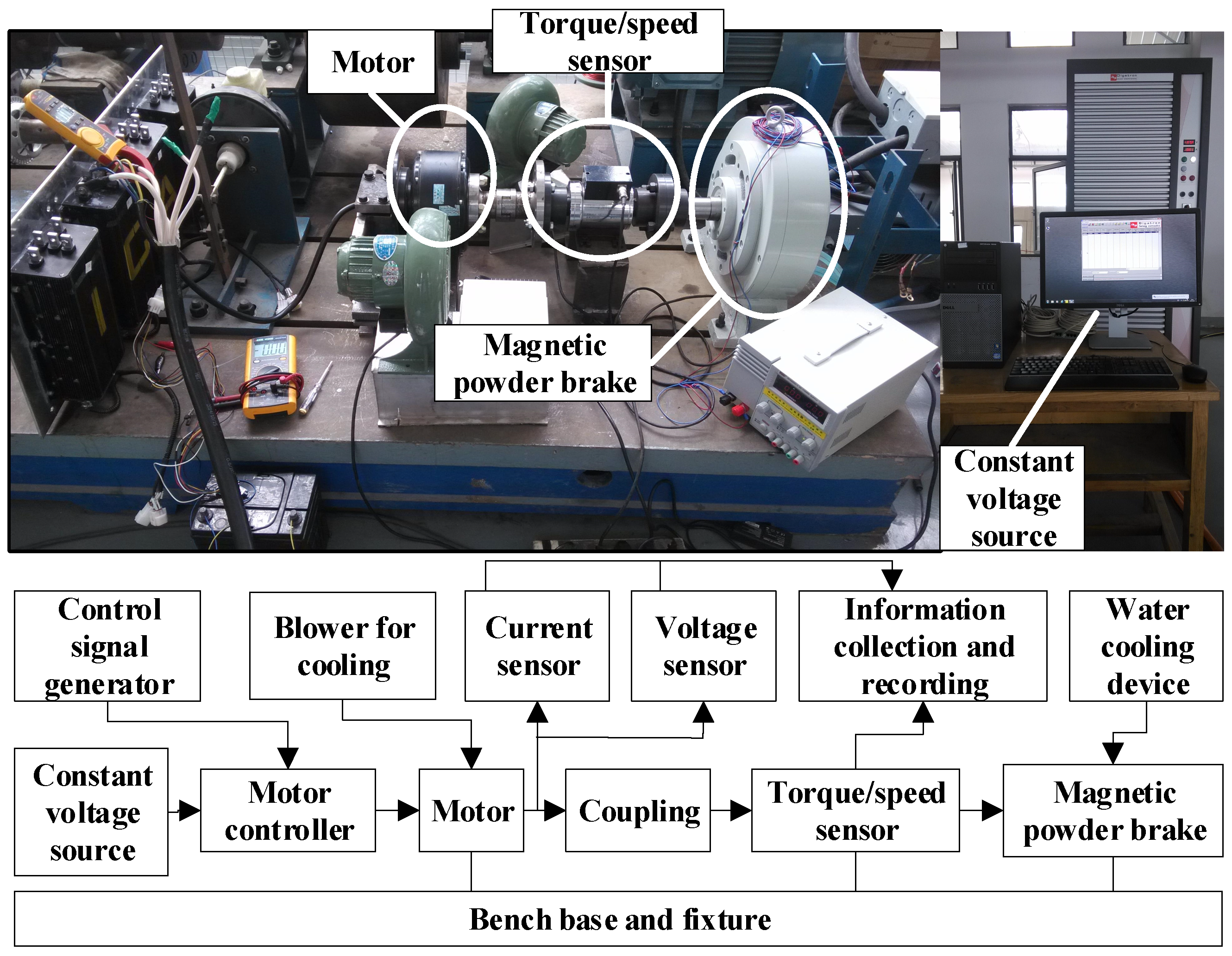
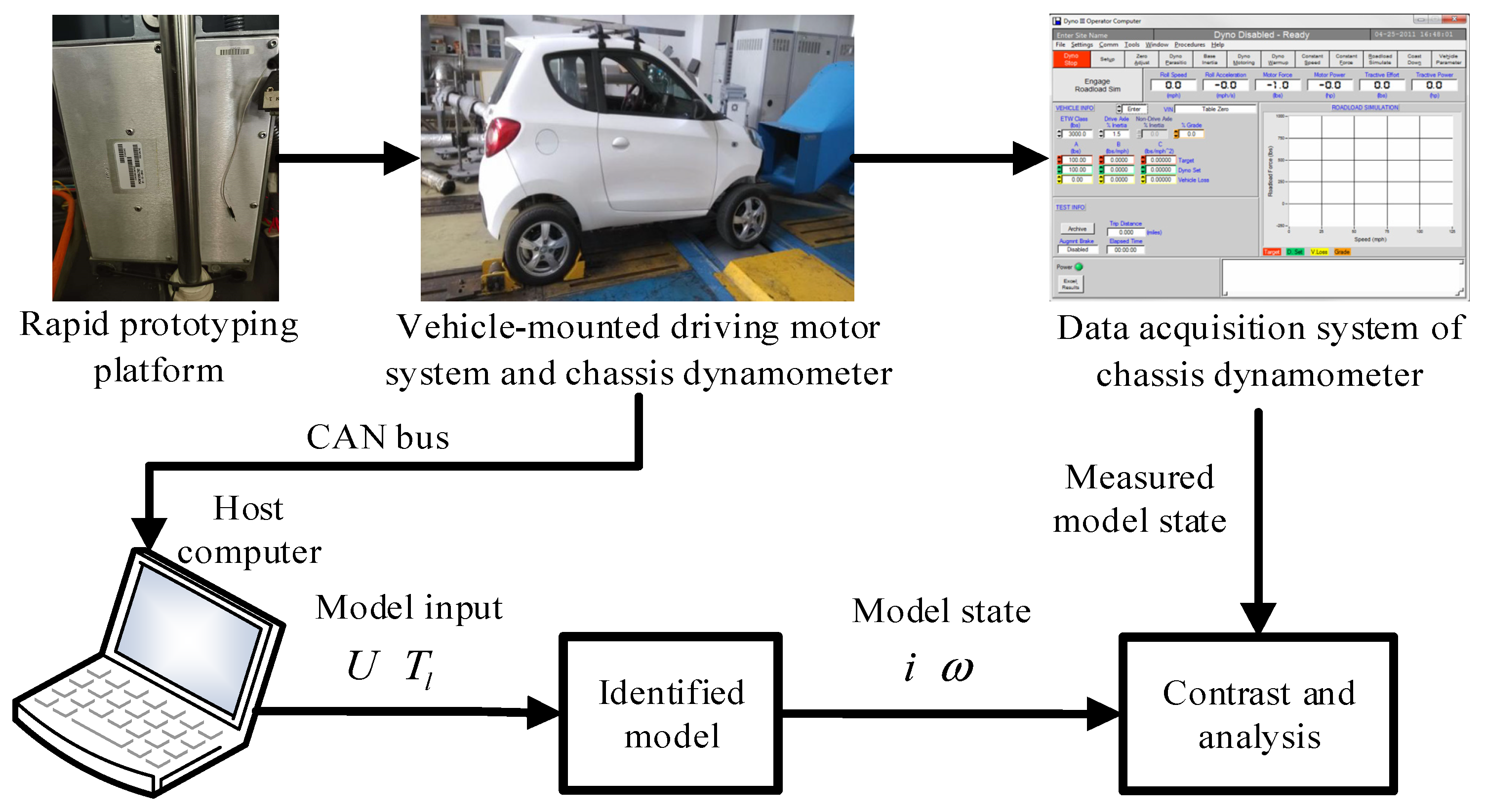
The chassis dynamometer simulation test of the vehicle-mounted permanent magnet DC brushless motor is shown in Figure 3. The test vehicle was a distributed drive electric vehicle modified from a micro pure electric vehicle, which uses four-wheel hub motors to directly drive the vehicle. D2P MotoHawk (Fort Collins, CO, USA) rapid prototype of version V2.4 is a software and hardware platform developed based on the product ECU and Matlab/Simulink control system. MotoHawk utilizes a product-level ECU hardware platform to enable the development of motor drive control systems without the need for user redevelopment. During the experiment, MotoHawk was used to establish a motor control model, and a certain control signal voltage was given to simulate the process from motor start-up to steady-state driving at a constant speed under the fixed power demand state of the motor. The front wheels of the vehicle were placed on the drum of the chassis dynamometer test bench, and the entire body of the vehicle was fixed. Then, by setting different pedal openings of the vehicle (corresponding to the motor controller signal voltage), the process of accelerating from a standstill when the motor had a load was simulated. The signal voltage of the motor controller was pre-set based on the rapid prototyping controller, which can avoid control signal fluctuations and unnecessary motor state fluctuations caused by the driver stepping on the pedal. We simulated the process of accelerating the vehicle from start to constant speed under different pedal openings by setting different motor control signal voltages. In addition, the chassis dynamometer system also has a dedicated blower to simulate the wind resistance of the vehicle at different wind speeds.

The current sensor and voltage sensor installed on the drive motor were used to monitor the bus current and bus voltage of the motor controller. The speed sensor at the wheel was a photoelectric speed sensor. When the wheel or motor rotated, it could convert the light pulses within the cycle into electrical pulses, thereby equivalently converting the motor speed based on the time required for the motor to rotate once. The motor torque was collected and converted through the chassis dynamometer system. At the same time, the CAN bus channel was used to record and save all sensor signals and controller signals. The vehicle SPY records and stores control signals and sensor signals on the vehicle bus.

The proposed algorithm was used for model identification and construction, and model validation was conducted after model identification with the aim of examining the fit between identification results and actual outputs. An input is applied to the data for the constructed identification model; a series of identification data is generated; and then these data are compared with the actual output data. Comparing the degree of fit between the state data curves of two sets of models provides an important basis for evaluating the accuracy of model identification.

The convergence stability of the identification model characterizes the accuracy of the model, as well as the reliability based on the model observer and controller. By observing the zero-pole distribution of the identification model system matrix, the stability of the model can be determined. If the zeros and poles of the model matrix are distributed within the unit circle of the complex plane, this system is considered stable. The zero pole distributions of the N4SID and PCA-N4SID model identification algorithms are (0.6503, 0.5672), (0.6368, −0.5613), and (0.6122, 0.5072), (0.5694, −0.5106), respectively, as shown in Figure 4. From this figure, it can be seen that the poles of both algorithms are within the unit circle, indicating that the identification models obtained are stable.

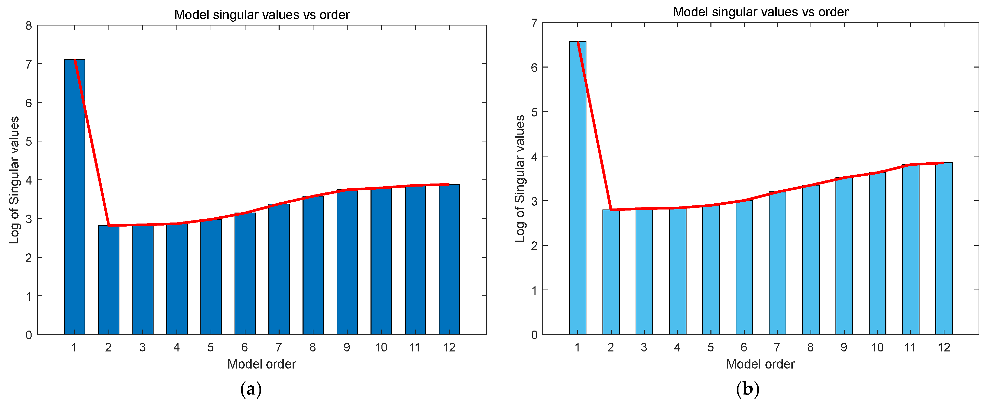
Singular value decomposition was performed on the constructed Hankel matrix by taking the first 12 singular values and calculating the logarithm. The relationship between the model order and the logarithm of the singular values is shown in Figure 5. According to this figure, the trend of singular value logarithms for both the N4SID and PCA-N4SID algorithms changes when the order is two. When the model order is one, the logarithm of singular values under both algorithms is relatively large. When the model order is two, the logarithm of singular values under both algorithms reaches the minimum value. As the order of the model gradually increases from two, the logarithm of singular values under both algorithms also gradually increases. The results indicate that when the model order is two, the logarithm of singular values under both algorithms reaches the minimum extremum point. Therefore, the model order of both the N4SID and PCA-N4SID algorithms can be determined as two.

The parameter set of {R, K_a, K_t, b, J, L} obtained based on the N4SID algorithm is {0.6632, 0.0637, 11.1952, 0.6206, 7.6581, 0.1293}. The parameter set of {R, K_a, K_t, b, J, L} obtained based on the PCA-N4SID algorithm is {0.6877, 0.0603, 11.4288, 0.6429, 7.1433, 0.1249}. Then, the identified model is used to validate its accuracy. Firstly, the model state identification results are validated without noise pollution, and the comparative results obtained are shown in Figure 6. As shown in the figure, the identification models obtained by both algorithms can track the actual system state as a whole, and both the current and speed values are in good agreement with the overall trend of the actual measurement result curve. At the same time, the model state curve under the PCA-N4SID algorithm is generally smoother, while the model state curve under the N4SID algorithm has some fluctuations. By zooming in on the local image, it can be seen more clearly that the PCA-N4SID algorithm has a higher performance following accuracy and real-time performance.

Before comparing different algorithms, it is important to emphasize the importance of mean squared error and average error in model evaluation. The average error reflects the degree of deviation between the predicted value and the true value of the model, which can intuitively reflect the accuracy of the model. The mean square error amplifies the impact of the error through the square operation, taking into account not only the size of the error but also its stability, which can more comprehensively reflect the performance of the model. By simultaneously analyzing the average error and mean square error, it is possible to more accurately evaluate the performance of the model under different operating conditions and provide a basis for algorithm improvement.

In order to further demonstrate the superiority of PCA-N4SID in model identification accuracy, a quantitative representation method was used to statistically analyze the average error and mean square error of identifying model state variables under N4SID and PCA-N4SID algorithms. The results are shown in

Table 1. Comparison of error quantification between two identification algorithms without noise pollution.

Method	Mean Error		Mean Square Error
	Current	Speed	Current	Speed
N4SID	2.4685	3.6861	2.9734	3.4964
PCA-N4SID	0.8627	1.0671	0.6119	0.8223

. According to the quantitative comparison results, the mean model errors of current and speed under the N4SID algorithm reached 2.4685 and 3.6861, respectively, while the mean model errors of current and speed under the PCA-N4SID algorithm were 0.8627 and 1.0671, respectively. The mean squared errors of the current and speed models under the N4SID algorithm reached 2.9734 and 3.4964, respectively, while the mean squared errors of the current and speed models under the PCA-N4SID algorithm were 0.6119 and 0.8223, respectively. It can be inferred that the mean and mean square error of the current and speed models under the PCA-N4SID algorithm were significantly smaller compared to those under the N4SID algorithm, and the effectiveness of the proposed model identification method was verified.

In practical applications, noise pollution has a significant impact on motor performance. Noise mainly comes from sensor accuracy limitations, electromagnetic interference, temperature changes, vibrations, and other factors. These noises can mask or distort the true characteristics of measurement data, resulting in the inaccurate extraction of effective information from the data. Specifically, noise pollution can cause deviations in the estimation of motor model parameters, making it difficult for the model to perform a number of functions, including accurately reflecting the actual characteristics of the motor, reducing the generalization ability of the model, which makes it difficult to make good predictions on new data; and it also leads to unstable estimation results of model parameters, making the model susceptible to external interference in practical applications and reducing its stability. Therefore, analyzing the noise pollution levels under different simulation conditions can provide important references for comparing identification algorithms and evaluating models.

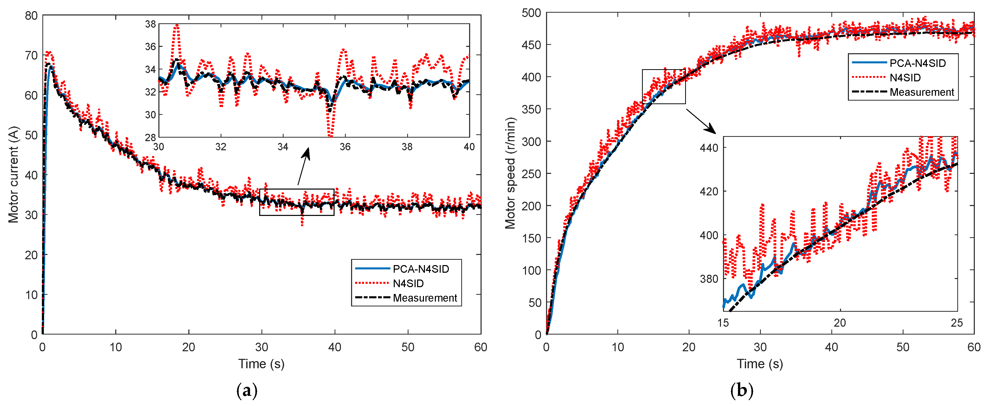
The model state identification results for when the input information contains 2% noise pollution are shown in Figure 7. The model state identified based on the N4SID algorithm shows that during the process of starting and accelerating the motor to a steady and uniform speed, the deviation of the motor current model is relatively large in the initial stage. This is because at the moment of motor start-up, the motor current increases sharply, the numerical fluctuation is relatively large, and then the motor speed also changes rapidly. In this state, the input of the model is relatively unstable, leading to deviations in the identification results of the model state. When the motor speed is stable, the accuracy of the identification model is relatively higher. Relatively speaking, the identification algorithm based on PCA-N4SID has higher accuracy throughout the entire process of motor start-up and has a stable trend, reflecting that the PCA-N4SID algorithm can suppress the negative impact of input signal fluctuations on model accuracy.

The comparison results of error quantification between two identification algorithms when the input information contains 2% noise pollution are shown in

Table 2. Comparison of error quantification between two identification algorithms under 2% noise pollution.

Method	Mean Error		Mean Square Error
	Current	Speed	Current	Speed
N4SID	3.1689	5.1983	3.7109	4.1284
PCA-N4SID	0.9167	1.1265	0.6613	0.8598

. In the quantitative comparison results, the mean model errors of current and speed under the N4SID algorithm reached 3.1689 and 5.1983, respectively, while the mean model errors of current and speed under the PCA-N4SID algorithm were 0.9167 and 1.1265, respectively. The mean squared errors of the current and speed models under the N4SID algorithm reached 3.7109 and 4.1284, respectively, while the mean squared errors of the current and speed models under the PCA-N4SID algorithm were 0.6613 and 0.8598, respectively. By comparison, it can be seen that under the condition of 2% noise pollution in the input information, the mean and mean square error of both identification algorithms increased. The current and speed errors increased more significantly under the N4SID algorithm, while the error values under the PCA-N4SID algorithm increased but still remained at the original level. In the case of signal noise pollution, the performance difference between N4SID and PCA-N4SID algorithms was more significant. The model state value error under the N4SID algorithm was relatively larger, while the error value under the PCA-N4SID algorithm was effectively controlled and did not significantly affect negative noise interference, thus verifying the fact that the PCA-N4SID algorithm can still maintain a good level of model identification accuracy under signal noise pollution.

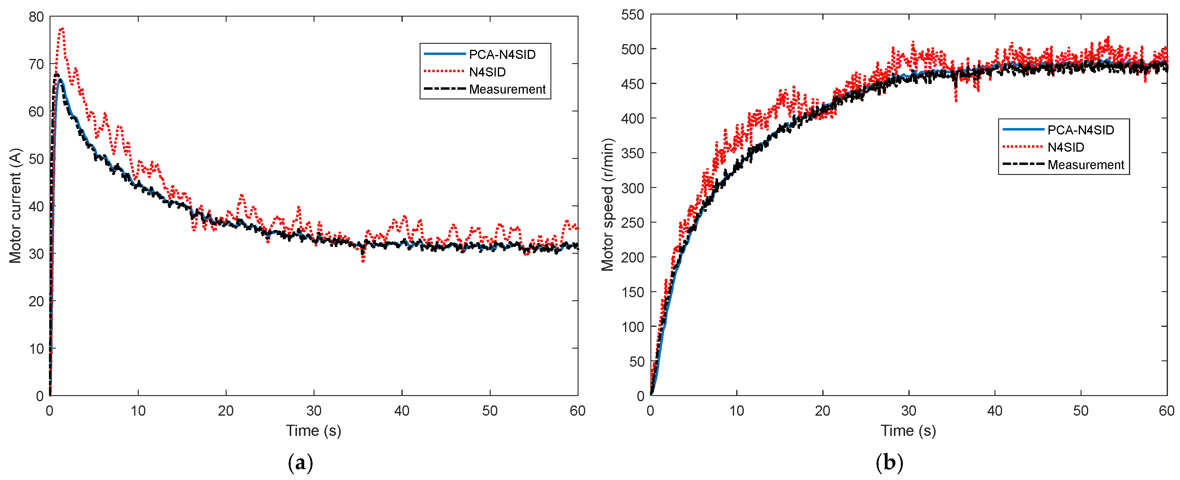
The model state identification results when the input information contains 5% noise pollution are shown in Figure 8. As shown in the figure, as the level of noise pollution in the input information increases, the error in the model state identification results based on the N4SID algorithm further increases, especially during the acceleration process of motor start-up. In contrast, the PCA-N4SID algorithm can still maintain its original identification accuracy, thus verifying its anti-interference ability and good real-time tracking characteristics.

The comparison results of error quantification between two identification algorithms for when the input information contains 5% noise pollution are shown in

Table 3. Comparison of error quantification between two identification algorithms under 5% noise pollution.

Method	Mean Error		Mean Square Error
	Current	Speed	Current	Speed
N4SID	5.2937	6.8802	4.3304	5.3111
PCA-N4SID	0.9504	1.3513	0.6965	0.9072

. In the quantitative comparison results, the mean model errors of current and speed under the N4SID algorithm reached 5.2937 and 6.8802, respectively, while the mean model errors of current and speed under the PCA-N4SID algorithm were 0.9504 and 1.3513, respectively. The mean squared errors of the current and speed models under the N4SID algorithm reached 4.3304 and 5.3111, respectively, while the mean squared errors of the current and speed models under the PCA-N4SID algorithm were 0.6965 and 0.9072, respectively. Comparing the data in Table 3, it can be seen that the mean and mean square deviation of the error under the N4SID algorithm doubled compared to the noise-free situation, while the mean and mean square deviation of the error under the PCA-N4SID algorithm remained at their original levels, further demonstrating the model identification performance of the PCA-N4SID algorithm compared to the N4SID algorithm under noise pollution.

5. Conclusions

In response to the problem of the model identification of permanent magnet DC brushless motors and considering the potential negative impact of noise pollution on data collection, this study proposes a data-driven method for the model identification of permanent magnet DC brushless motors based on the auxiliary variable closed-loop subspace identification algorithm. To effectively weaken the correlation between input signals and noise, based on an error variable model, auxiliary variables are introduced to avoid the projection step of traditional subspace identification algorithms, and the algorithm’s implementation is optimized in the principal component analysis stage to simplify the solution process. The results indicate that the proposed PCA-N4SID algorithm can effectively handle the situation where driving data are contaminated by noise, and compared to the N4SID algorithm, the model identification accuracy was significantly improved.

In future research, the identification of motor models will present a multidimensional development trend. Intelligent and adaptive modeling will deeply integrate deep learning algorithms, utilizing their powerful feature extraction capabilities to automatically mine complex patterns in motor operation data. At the same time, adaptive modeling technology will be further developed, enabling models to be updated in real time to adapt to the dynamic characteristics of motors under different working conditions and load conditions. Multi-physics coupling modeling will pay more attention to the interaction of multiple fields in physics, such as electromagnetic, thermal, and mechanical fields. By establishing a unified multi-physics field model, the actual operating state of the motor can be more comprehensively reflected and the accuracy and reliability of the model can be improved. The application of digital twin technology will bring new development opportunities for motor model identification. By constructing the digital twin models of motors, real-time interaction and data sharing between physical motors and virtual models can be achieved, enabling a more accurate performance evaluation, fault prediction, and optimized control of motors.

The research on motor model identification will continue to expand in three directions: model-driven identification, data-driven identification, and model-data-fusion-driven identification. Model-driven identification will focus on fine-grained and multi-physics field-coupling modeling, combined with advanced numerical calculation methods, to more accurately describe the complex physical phenomena and interactions inside the motor, such as the coupling effects of electromagnetic fields, temperature fields, and stress fields. Data-driven identification will become more precise with the development of big data and artificial intelligence technologies, and deep learning algorithms will be widely used to mine complex patterns and nonlinear relationships in the data. The fusion of models and data-driven identification will become an important development direction. By combining prior knowledge, and the physical constraints driven by models with actual measurement data and using methods such as physical information neural networks to achieve deep fusion, more accurate and reliable motor models can be established, thus promoting the progress of motor model identification technology.

References

1. Bu, W.; Fan, Z.; Zhang, J.; Tao, W. Research on the Bearingless Brushless DC Motor Structure with Like-Tangential Parallel-Magnetization Interpolar Magnetic Poles and Its Air-Gap Magnetic Field Analytical Calculation. Actuators 2025, 14, 198. [Google Scholar] [CrossRef]
2. Lian, C.; Xiao, F.; Liu, J.; Gao, S. Parameter and VSI Nonlinearity Hybrid Estimation for PMSM Drives Based on Recursive Least Square. IEEE Trans. Transp. Electrif. 2023, 9, 2195–2206. [Google Scholar] [CrossRef]
3. Mi, M.; Che, Y.; Li, H.; Zhao, S. Identification of Rotor Position of Permanent Magnet Spherical Motor Based on Compressed Sensing. IEEE Trans. Ind. Inform. 2023, 19, 9157–9164. [Google Scholar] [CrossRef]
4. Gan, H.; Cao, Z.; Chen, P.; Luo, Y.; Luo, X. Fractional-Order Electromagnetic Modeling and Identification for PMSM Servo System. ISA Trans. 2024, 147, 527–539. [Google Scholar] [CrossRef]
5. Beltran-Carbajal, F.; Tapia-Olvera, R.; Valderrabano-Gonzalez, A.; Yanez-Badillo, H.; Rosas-Caro, J.; Mayo-Maldonado, J. Closedloop Online Harmonic Vibration Estimation in DC Electric Motor Systems. Appl. Math. Model. 2021, 94, 460–481. [Google Scholar] [CrossRef]
6. Cetinceviz, Y. Optimal Design, Electromagnetic–Thermal Analysis and Application of In-Wheel Permanent Magnet BLDC Motor for E-Mobility. Appl. Sci. 2025, 15, 3258. [Google Scholar] [CrossRef]
7. Zhang, S.; Zhou, Z.; Pu, Y.; Li, Y.; Xu, Y. Parameter Identification of Permanent Magnet Synchronous Motor Based on LSOSMO Algorithm. Sensors 2025, 25, 2648. [Google Scholar] [CrossRef]
8. Manoharan, P.; Ravichandran, S.; Siva Kumar, J.S.V.; Abdullah, M.; Ching Sin, T.; Tengku Hashim, T.J. Electrical Equivalent Circuit Parameter Estimation of Commercial Induction Machines Using an Enhanced Grey Wolf Optimization Algorithm. Biomimetics 2025, 10, 228. [Google Scholar] [CrossRef]
9. Huang, S.; Zhang, Y.; Shi, L.; Huang, Y.; Chang, B. Dual-Vector-Based Model Predictive Current Control with Online Parameter Identification for Permanent-Magnet Synchronous Motor Drives in Marine Electric Power Propulsion System. J. Mar. Sci. Eng. 2025, 13, 585. [Google Scholar] [CrossRef]
10. Amador, S.D.R.; Brincker, R. The new subspace-based poly-reference complex frequency (S-pCF) for robust frequency-domain modal parameter estimation. Measurement 2024, 225, 113995. [Google Scholar] [CrossRef]
11. Wang, Y.; Zhang, L.; Zhao, Y. Improved closed-loop subspace identification with prior information. Int. J. Syst. Sci. 2018, 49, 1821–1835. [Google Scholar] [CrossRef]
12. She, M.; Ding, B. Closed-loop subspace identification of multivariable dynamic errors-in-variables models based on ORT. Clust. Comput 2019, 22 (Suppl. 2), 4907–4915. [Google Scholar] [CrossRef]
13. Wang, Q.; Liu, S.; Zhang, G.; Ding, D.; Li, B.; Wang, G.; Xu, D. Zero-Sequence Voltage Error Elimination-Based Offline VSI Nonlinearity Identification for PMSM Drives. IEEE Trans. Transp. Electrif. 2024, 10, 55–66. [Google Scholar] [CrossRef]
14. Paula, M.V.D.; Ricco, R.A.; Teixeira, B.O.S. Subspace identification of Hammerstein models with interval uncertainties. J. Process Control 2025, 149, 103412. [Google Scholar] [CrossRef]
15. Wu, J.-D.; Luo, W.-J.; Yao, K.-C. Electric Motor Vibration Signal Classification Using Wigner-Ville Distribution for Fault Diagnosis. Sensors 2025, 25, 1196. [Google Scholar] [CrossRef] [PubMed]
16. Pei, T.H.; Li, D.W.; Liu, J.Y.; Li, J. Review of bearingless synchronous motors: Principle and topology. IEEE Trans. Transp. Electrif. 2022, 8, 3489–3502. [Google Scholar] [CrossRef]
17. Bian, Y.F.; Yang, Z.B.; Sun, X.D.; Wang, X. Speed sensorless control of a bearingless induction motor based on modified robust kalman filter. J. Electr. Eng. Technol. 2024, 19, 1179–1190. [Google Scholar] [CrossRef]
18. Xu, E.X.; Zhao, R.J. Research on Displacement Sensorless Control for Bearingless Synchronous Reluctance Motor Based on the Whale Optimization Algorithm-Elman Neural Network. Actuators 2024, 13, 192. [Google Scholar] [CrossRef]
19. Li, K.; Luo, H.; Yang, C.; Yin, S. Subspace-Aided Closed-Loop System Identification and Its Application to DC Motor Systems. IEEE Trans. Ind. Electron. 2020, 67, 2304–2313. [Google Scholar] [CrossRef]
20. Masoud, A.A.; Abu-Ali, M.; Al-Shaikhi, A. A Novel and Effective Protocol for State-Space Model Identification: An Undergraduate First Control Laboratory Education. In Proceedings of the American Control Conference (ACC), Milwaukee, WI, USA, 27–19 June 2018; pp. 4843–4848. [Google Scholar]
21. Li, K.; Luo, H.; Jiang, Y.; Tang, D.; Yang, H. Subspace Identification for Closed-Loop Systems with Unknown Deterministic Disturbances. IEEE/CAA J. Autom. Sin. 2023, 10, 2248–2257. [Google Scholar] [CrossRef]
22. Bu, W.S.; Li, H. Torque System Modeling and Electromagnetic Coupling Characteristics Analysis of a Midpoint Injection Type Bearingless Permanent Synchronous Magnet Motor. Int. Trans. Electr. Energy Syst. 2024, 2024, 3078894. [Google Scholar] [CrossRef]
23. Zhu, H.Q.; Hao, Z.J.; Pan, W.; Diao, X. Research, Application and Development Trends of Bearingless Brushless DC Motor. Trans. China Electrotech. Soc. 2019, 34, 4428–4440. [Google Scholar]
24. Wang, Y.; Zhan, H.; Gong, Y.; Wang, M.; Yu, J.; Zhang, Z.; Yang, Y.; Wang, L. Demagnetization Analysis and Optimization of Bonded Nd-Fe-B Magnet Rings in Brushless DC Motors. Machines 2025, 13, 75. [Google Scholar] [CrossRef]
25. Banerjee, S.; Saravanan, T.J. Robust data-driven online learning algorithm for precise structural damage localization using stochastic subspace identification. Measurement 2025, 244, 116536. [Google Scholar] [CrossRef]
26. Liu, Q.; Liu, T.; Huang, D.; Shang, C. Subspace identification of dynamic processes with consideration of time delays: A Bayesian optimization scheme. J. Process Control 2025, 147, 103387. [Google Scholar] [CrossRef]
27. Fu, C.; Jiang, C.; Wan, Z.; Wang, Q.; Wang, S. A robust distributed fault detection scheme for interconnected systems based on subspace identification technique. Control Eng. Pract. 2025, 159, 106301. [Google Scholar] [CrossRef]
28. Tang, Y.; Ding, J.; Chen, Y.; Gao, Y.; Jiang, A.; Wang, C. Anxiety disorder identification with biomarker detection through subspace-enhanced hypergraph neural network. Neural Netw. 2025, 187, 107293. [Google Scholar] [CrossRef]
29. Tomassini, E.; García-Macías, E.; Ubertini, F. Fast stochastic subspace identification of densely instrumented bridges using randomized SVD. Mech. Syst. Signal Process. 2025, 225, 112264. [Google Scholar] [CrossRef]
30. Yu, Z.; Huang, Z.; Hou, M.; Pei, J.; Sun, D. Inter-block ladder-style transformer model with multi-subspace feature adjustment for object re-identification. Appl. Soft Comput. 2025, 174, 112961. [Google Scholar] [CrossRef]
31. Qiu, Z.J.; Ma, D.X.; Wei, K.N. Optimization Analysis on Suspension Control Characteristics of a Bearingless Brushless DC Motor. Trans. China Electrotech. Soc. 2019, 34, 4939–4947. [Google Scholar]
32. Liu, Y.C.; Zhu, H.Q.; Xu, B. Mathematical modelling and control of bearingless brushless direct current machine with motor and generator double modes for flywheel battery. IET Power Electron. 2022, 15, 1249–1263. [Google Scholar] [CrossRef]
33. Shang, X.; Li, W.; Yuan, F.; Zhi, H.; Gao, Z.; Guo, M.; Xin, B. Research on Fault Diagnosis of UAV Rotor Motor Bearings Based on WPT-CEEMD-CNN-LSTM. Machines 2025, 13, 287. [Google Scholar] [CrossRef]
34. Cui, Z.S.; Zhou, Y.Z.; Zhou, Y.H. Analytical calculation of magnetic field of dual-winding bearingless flux-switching permanent magnet motors baseds on improved subdomain model. Electr. Mach. Control 2022, 26, 66–67. [Google Scholar]
35. Cheng, W.; Cao, G.; Deng, Z.; Ling, X.; Ming, L. Torque comparison between slotless and slotted ultra-high-speed AFPM motors using analytical method. IEEE Trans. Magn. 2021, 58, 3081175. [Google Scholar] [CrossRef]
36. Beltran-Carbajal, F.; Silva-Navarro, G.; Trujillo-Franco, L.G. On-line parametric estimation of damped multiple frequency oscillations. Electr. Power Syst. Res. 2018, 154, 423–432. [Google Scholar] [CrossRef]
37. Ding, J.; Chen, L.; Cao, Z.; Guo, H. Convergence Analysis of the Modified Adaptive Extended Kalman Filter for the Parameter Estimation of a Brushless DC Motor. Int. J. Robust Nonlinear Control 2021, 31, 7606–7620. [Google Scholar] [CrossRef]
38. Che, Z.; Yu, H.; Mobayen, S.; Ali, M.; Yang, C.; Bartoszewicz, A. An improved extended state observer-based composite nonlinear control for permanent magnet synchronous motor speed regulation systems. Energies 2022, 15, 5699. [Google Scholar] [CrossRef]
39. Su, G.; Wang, P.; Guo, Y.; Cheng, G.; Wang, S.; Zhao, D. Multiparameter Identification of Permanent Magnet Synchronous Motor Based on Model Reference Adaptive System-Simulated Annealing Particle Swarm Optimization Algorithm. Electronics 2022, 11, 159. [Google Scholar] [CrossRef]
40. Lyu, B.; Jia, L.; Li, F. Neuro-fuzzy based identification of Hammerstein OEAR systems. Comput. Chem. Eng. 2020, 141, 106984. [Google Scholar] [CrossRef]
41. Wang, H.; Zhang, Q.; Liu, X. Auxiliary model-based maximum likelihood multi-innovation recursive least squares identification for multiple-input multiple-output systems. J. Frankl. Inst. 2024, 361, 107352. [Google Scholar] [CrossRef]
42. Zhang, L.; Zhou, D.; Zhong, M.; Wang, Y. Improved closed-loop subspace identification based on principal component analysis and prior information. J. Process Control 2019, 80, 235–246. [Google Scholar] [CrossRef]
43. Ramnath, K.; Narasimhan, S. Identification of errors in variables linear state space models using iterative principal component analysis. Int. J. Control 2022, 6, 2773–2786. [Google Scholar] [CrossRef]
44. Gör, H. Feasibility of Six Metaheuristic Solutions for Estimating Induction Motor Reactance. Mathematics 2024, 12, 483. [Google Scholar] [CrossRef]
45. Huo, M.; Luo, H.; Cheng, C.; Li, K.; Yin, S.; Kaynak, O. Subspace-Aided Sensor Fault Diagnosis and Compensation for Industrial Systems. IEEE Trans. Ind. Electron. 2023, 70, 9474–9482. [Google Scholar] [CrossRef]
Figure 1. Schematic diagram of the motor characteristic test.
Wevj 16 00297 g001
Figure 2. Motor characteristic data under different line voltages: (a) motor speed torque curve, (b) motor speed current curve, and (c) motor torque current curve.
Wevj 16 00297 g002
Figure 3. Simulation test of chassis dynamometer for vehicle-mounted permanent magnet brushless DC motor.
Wevj 16 00297 g003
Figure 4. Zero-pole distribution of two identification algorithms. (a) N4SID algorithm; (b) PCA-N4SID algorithm.
Wevj 16 00297 g004
Figure 5. The model order and singular value logarithm under two identification algorithms. (a) N4SID algorithm; (b) PCA-N4SID algorithm.
Wevj 16 00297 g005
Figure 6. Model state identification results without noise pollution: (a) current value; (b) speed value.
Wevj 16 00297 g006
Figure 7. Model state identification results for under 2% noise pollution: (a) current value; (b) speed value.
Wevj 16 00297 g007
Figure 8. Model state identification results for under 5% noise pollution: (a) current value; (b) speed value.
Wevj 16 00297 g008