Road Feel Simulation Strategy for Steer-by-Wire System in Electric Vehicles Based on an Improved Nonlinear Second-Order Sliding Mode Observer

Abstract

Addressing the shortcoming that steer-by-wire (SBW) system cannot directly transmit road feel, this study investigates a SBW system dynamics model, steering angle tracking control, and road feel simulation algorithm design. This study proposes a high-precision observer-based road feel simulation method that achieves road feel feedback torque design through the real-time estimation of system disturbance torque based on accurate front-wheel angle tracking. The methodology employs an improved nonlinear second-order sliding mode observer (INSOSMO) to estimate the system disturbance torque. This observer incorporates proportional–integral terms into the super-twisting algorithm to enhance dynamic response, replaces the sign function with a Sigmoid function to eliminate chattering, and utilizes the sparrow search algorithm (SSA) for global parameter optimization. Meanwhile, a two-stage filter combining a strong tracking Kalman filter (STKF) and first-order low-pass filtering processes the observer values to generate road feel feedback torque. Additionally, for the active return control of the steering wheel, a backstepping sliding mode control (BSSMC) integrated with an extended state observer (ESO) is employed, where the ESO enhances the robustness of BSSMC through real-time nonlinear disturbance estimation and compensation. MATLAB/Simulink-CarSim co-simulation demonstrates that, under sinusoidal testing, the INSOSMO reduces mean absolute error (MAE) by 34.7%, 62.5%, and 60.1% compared to the ESO, Kalman filter observer (KFO), and conventional sliding mode observer (SMO), respectively. The designed road feel feedback torque meets operational requirements. The active return controller maintains accurate steering wheel repositioning across various speed ranges.

1. Introduction

The SBW system has emerged as the preferred steering solution for next-generation advanced intelligent vehicles due to its distinctive advantages [1]. Through mechanical decoupling between the steering wheel and wheels, SBW enables the independent design of force transmission and angle response characteristics, significantly enhancing compatibility with intelligent and connected vehicle architectures [2,3,4]. However, at this stage, it is difficult to realize fully autonomous driving technology. The driver still has to participate in the driving process, and the automobile human–machine interface cannot be completely removed [5]. Due to the special characteristics of its structure, the SBW system is unable to transmit road feel directly through a mechanical connection [6,7], and needs to generate road feel through a road feel simulation device in order to ensure that the driver can accurately perceive road information in real time (the main components include steering load, system inertia, and frictional torque, among others), thus ensuring driving safety [8,9]. Therefore, the study of road feel simulation is indispensable.

Current research on road feel simulation for SBW systems primarily focuses on road feedback torque planning, with extended studies on the active return control of the steering wheel based on this foundation [10,11]. Current research on road feel feedback torque planning primarily focuses on emulating the road feel characteristics of electric power steering (EPS) systems, with two main approaches being adopted: model-based methods (implemented through tire–vehicle dynamics models or observers) and data-driven methods. Among these approaches, tire modeling-based methods suffer from inherent limitations, such as challenging parameter identification and poor environmental adaptability. Consequently, observer-based methods are increasingly emerging as a research focus due to their superior engineering feasibility. Shi et al. developed a terminal sliding mode observer to estimate the rack force in an SBW system, based on which the road feel feedback torque was designed. Simultaneously, they achieved precise control of the road feel motor using active disturbance rejection control. Vehicle experiments demonstrated the effectiveness of the proposed algorithms [12]. Su et al. designed an ESO to estimate rack force, and developed a personalized road feel feedback torque model by leaving some parameters adjustable [13]. Zheng et al. used a KFO to estimate the rack force of the steering system and added assist torque to design a road feel torque planning method for SBW systems with the goal of replicating the road feel of the EPS system, and the experimental results showed that the designed road feel torque improved the maneuverability and comfort of the car [14]. Regarding data-driven methods, Liu et al. developed a data-driven road feel feedback torque model using a CNN-GRU hybrid neural network architecture, and achieved the accurate tracking of desired torque through explicit model predictive control [15]. Zhao et al. collected road feel torque data from four common driving scenarios, utilized K-Means clustering, analyzed the training dataset, and selected a Gaussian process regression model to train the data in order to obtain road feel information [16]. Data-driven methods can holistically incorporate various factors affecting road feel to achieve more authentic steering feedback design. However, these approaches present inherent trade-offs between model fidelity and implementation practicality, while requiring substantial real-world vehicle test data for model development and validation. Based on the aforementioned research background, how to improve observer estimation accuracy while providing drivers with real-time and accurate road information has become a key scientific challenge in the field of steering feel simulation [17,18]. It should be noted that some observed values from the observer may contain invalid information, making the effective filtering of these interference components another important research issue. To address this challenge, this study proposes a road feel feedback torque design method based on a high-precision disturbance observer. By developing a dedicated filter to optimize the observed values, the proposed approach ensures the precise transmission of road information while further enhancing driving comfort.

Steering wheel active return should also be considered as one of the key aspects in road feel simulation. For steering wheel return control, the steering wheel return performance of the SBW system is related to the maneuvering stability of the car, and poor return performance will increase the driver’s driving burden and reduce driving pleasure [19]. Xie et al. considered that the automobile self-aligning torque could be significantly reduced on low-adhesion road surfaces, estimated the road-surface adhesion coefficient using the extended Kalman filter, and designed a time-varying sliding mode control algorithm to output different return currents according to different road-surface adhesion coefficients in order to improve the return performance of automobiles on low-adhesion road surfaces [9]. Zhao et al. proposed an active return control strategy for steering wheels based on sliding mode control (SMC), and a hardware-in-the-loop test showed that the designed control strategy could effectively reduce the return margin angle and improve the maneuvering stability of the car [11]. In addition, Chen et al. realized the active return control of steering wheels based on the fuzzy logic control algorithm [20]. Conventional steering wheel active return control strategies often overlook inherent system disturbances and parameter uncertainties. However, nonlinear disturbances can significantly degrade steering return performance, causing positioning inaccuracies that are fundamentally unacceptable for SBW system applications. Therefore, how to enable control algorithms to possess nonlinear disturbance compensation capabilities and thereby enhance their robustness has become a core research focus in this field.

In this study, a novel road feel simulation strategy based on an INSOSMO is proposed. The main contributions of this study are as follows:

(1)

An INSOSMO is developed for high-precision state estimation: The observer is constructed based on the super-twisting algorithm. The approach incorporates both proportional and integral terms into the super-twisting algorithm, replaces the conventional sign function with an improved Sigmoid function to suppress chattering, and employs the SSA for the global optimization of key parameters. Comparative experiments demonstrate significantly improved observation accuracy over conventional ESO, KFO, and SMO approaches.

(2)

A two-stage filter is proposed to eliminate extraneous components in road feel feedback torque: The filter combines STKF with a first-order low-pass filter to process the observed values from the INSOSMO. Based on the filtered results, the main road feel torque is designed, which is then superimposed with compensation torque to generate the final road feel feedback torque.

(3)

Considering steering wheel return control, a steering wheel active return controller accounting for system disturbances is developed: Based on hybrid algorithm theory, the controller employs BSSMC as its core algorithm. To address nonlinear disturbances in the system, an ESO is designed for observation and compensation, thereby enhancing the controller’s robustness.

2. Dynamics Model of the SBW System

The structure of the SBW system is schematically shown in Figure 1.

Working Principle of SBW System: The driver inputs steering commands by rotating the steering wheel. The Electronic Control Unit (ECU) then calculates the target steering angle by integrating the vehicle’s motion state and driver inputs via a predefined algorithm. Next, the steering angle tracking control algorithm determines the required torque for the steering actuator motor to achieve the desired motion, driving the motor to execute steering. Simultaneously, the ECU generates road feel feedback torque based on vehicle speed, road conditions, and real-time steering wheel status, simulating force feedback through a motor to provide the driver with realistic road feel for precise vehicle control [21,22,23].

2.1. Dynamics Model of the Steering Wheel Subsystem

The steering-wheel-to-torque-sensor dynamics equation can be expressed as

$$\left\{\begin{array}{c}{T}_{\mathrm{h}}=J_{\mathrm{sw}}{\ddot{\theta }}_{\mathrm{sw}}+B_{\mathrm{sw}}{\dot{\theta }}_{\mathrm{sw}}+K_{\mathrm{f}}\mathsf{\Delta }{\theta }_{\mathrm{f}}+T_{\mathrm{fh}}\\ \mathsf{\Delta }{\theta }_{\mathrm{f}}=\left({\theta }_{\mathrm{sw}}-{\displaystyle \frac{{\theta }_{\mathrm{f}}}{G_{\mathrm{f}}}}\right)\end{array}\right.,$$

(1)

The road feel motor dynamics equation can be expressed as

$$T_{\mathrm{f}}=J_{\mathrm{f}}{\ddot{\theta }}_{\mathrm{f}}+B_{\mathrm{f}}{\dot{\theta }}_{\mathrm{f}}-{\displaystyle \frac{K_{\mathrm{f}}\mathsf{\Delta }{\theta }_{\mathrm{f}}}{G_{\mathrm{f}}}}+T_{\mathrm{ff}},$$

(2)

where T_h is the driver input torque; θ_sw is the steering wheel angle; J_sw is the rotational inertia of the steering column; B_sw is the damping coefficient of the steering column; K_f is the stiffness coefficient of the torque sensor; θ_f is the rotation angle of the road feel motor; G_f is the reduction ratio; T_fh is the equivalent friction torque; T_f is the electromagnetic torque of the road feel motor; J_f is the rotational inertia of the road feel motor; B_f is the damping coefficient of the road feel motor; and T_ff is the equivalent frictional torque of the road feel motor.

2.2. Dynamics Model of the Steering Actuation Subsystem

The dynamic equation of the steering actuator motor can be expressed as follows:

$$\left\{\begin{array}{c}{T}_{\mathrm{m}}=J_{\mathrm{m}}{\ddot{\theta }}_{\mathrm{m}}+B_{\mathrm{m}}{\dot{\theta }}_{\mathrm{m}}+K_{\mathrm{m}}\mathsf{\Delta }{\theta }_{\mathrm{m}}/G_{\mathrm{m}}+T_{\mathrm{mm}}\\ \mathsf{\Delta }{\theta }_{\mathrm{m}}=\left({\displaystyle \frac{{\theta }_{\mathrm{m}}}{G_{\mathrm{m}}}}-{\displaystyle \frac{x_{\mathrm{r}}}{r_{\mathrm{p}}}}\right)\end{array}\right.,$$

(3)

where T_m is the electromagnetic torque of the steering actuator motor; J_m is the rotational inertia of the steering actuator motor; B_m is the damping coefficient of the steering actuator motor; K_m is the torsional stiffness of the steering actuator assembly; θ_m is the steering actuator motor angle; G_m is the reduction ratio; x_r is the rack displacement; r_p is the pinion radius; and T_mm is the equivalent friction torque of the steering actuator motor.

Then, the model of the rack-and-pinion steering gear section is established. In this section, the torque applied by the steering actuator motor to the motor shaft serves as the input. After being transmitted through the reducer, it drives the rack and pinion steering mechanism, ultimately enabling the steering wheels to complete the turning motion. Therefore, the dynamic equation can be expressed as follows:

$$\left\{\begin{array}{c}{M}_{\mathrm{r}}{\ddot{x}}_{\mathrm{r}}+B_{\mathrm{r}}{\dot{x}}_{\mathrm{r}}+F_{\mathrm{rack}}+F_{\mathrm{f}}={\displaystyle \frac{K_{\mathrm{f}}\mathsf{\Delta }{\theta }_{\mathrm{f}}}{r_{\mathrm{p}}}}\\ F_{\mathrm{rack}}={\displaystyle \frac{T_{\mathrm{fw}}}{i_{\mathrm{fw}}}}={\displaystyle \frac{T_{\mathrm{fw}}}{i_{\mathrm{sw}}{r}_{\mathrm{p}}}}\end{array}\right.,$$

(4)

where M_r is the quality of the rack-and-pinion steering gear; B_r is the damping coefficient of the rack-and-pinion steering gear; F_rack is the rack force; F_f is the equivalent friction force on the rack-and-pinion steering gear; T_fw is the torque acting on the kingpin axis originating from the tires; and i_fw is the transmission ratio from the rack to the steering knuckle arm. i_sw is the steering system transmission ratio.

The dynamic equation of the steering wheel is

$$T_{\mathrm{fw}}=J_{\mathrm{fw}}{\ddot{\theta }}_{\mathrm{fw}}+B_{\mathrm{fw}}{\dot{\theta }}_{\mathrm{fw}}+T_{\mathrm{sa}}+T_{\mathrm{fwf}},$$

(5)

where J_fw is the rotational inertia of the front wheel; θ_fw is the steering angle of the front wheel; B_fw is the damping coefficient of the front wheel; T_sa is the self-aligning torque of the front wheel; and T_fwf is the equivalent friction torque of the front wheel.

2.3. Design of the Steering Angle Tracking Algorithm

Precise steering angle tracking control serves as the fundamental prerequisite for road feel feedback torque planning in SBW system. This study develops a steering angle tracking controller based on a nonsingular fast terminal sliding mode control (NFTSMC) algorithm to guarantee accurate wheel response to driver commands. The second-order equivalent model of the SBW system’s steering actuation subsystem is derived from Equations (3)–(5), as follows:

$$T_{\mathrm{eq}}=J_{\mathrm{eq}}{\ddot{\theta }}_{\mathrm{fw}}+B_{\mathrm{eq}}{\dot{\theta }}_{\mathrm{fw}}+T_{\mathrm{sa}}+T_{\mathrm{f}},$$

(6)

where

$$\left\{\begin{array}{l}K={\displaystyle \frac{G_{\mathrm{m}}{i}_{\mathrm{fw}}}{r_{\mathrm{p}}}}\\ T_{\mathrm{eq}}=K{T}_{\mathrm{m}}\\ J_{\mathrm{eq}}=K^2{J}_{\mathrm{m}}+{i_{\mathrm{fw}}}^2{M}_{\mathrm{r}}+J_{\mathrm{fw}}\\ B_{\mathrm{eq}}=K^2{B}_{\mathrm{m}}+{i_{\mathrm{fw}}}^2{B}_{\mathrm{r}}+B_{\mathrm{fw}}\\ T_{\mathrm{f}}=i_{\mathrm{fw}}{F}_{\mathrm{f}}+T_{\mathrm{fwf}}+K{T}_{\mathrm{mm}}\end{array}\right.,$$

(7)

where J_eq is the equivalent rotational inertia; B_eq is the equivalent damping coefficient; and T_f is the system friction torque.

Let $x={[\begin{array}{cc}{x}_1& x_2\end{array}]}^{\mathrm{T}}={\left[\begin{array}{cc}{\theta }_{\mathrm{fw}}& {\dot{\theta }}_{\mathrm{fw}}\end{array}\right]}^{\mathrm{T}}$ and u = T_eq. From Equation (6), the state-space equation is derived as follows:

$$\left\{\begin{array}{l}{\dot{x}}_1=x_2\\ {\dot{x}}_2={\displaystyle \frac{1}{J_{\mathrm{eq}}}}u-{\displaystyle \frac{B_{\mathrm{eq}}}{J_{\mathrm{eq}}}}{x}_2-{\displaystyle \frac{1}{J_{\mathrm{eq}}}}d\\ d=\mathsf{\Delta }{J}_{\mathrm{eq}}{\dot{x}}_2+\mathsf{\Delta }{B}_{\mathrm{eq}}{x}_2+T_{\mathrm{sa}}+T_{\mathrm{f}}\end{array}\right.,$$

(8)

where d satisfies $d\le \left|D\right|$.

Define the angle error as e_δ = x₁ − z_d, where z_d is the desired front wheel steering angle. The first and second derivatives of e_δ can then be expressed as

$${\dot{e}}_{\mathsf{\delta }}=x_2-{\dot{z}}_{\mathrm{d}},$$

(9)

$${\ddot{e}}_{\mathsf{\delta }}={\dot{x}}_2-{\ddot{z}}_{\mathrm{d}},$$

(10)

The nonsingular fast terminal sliding mode surface is constructed as

$$s_{\mathsf{\delta }}=e_{\mathsf{\delta }}+\alpha \mathrm{sign}({\dot{e}}_{\mathsf{\delta }}){\left|{\dot{e}}_{\mathsf{\delta }}\right|}^{{\displaystyle \frac{p}{q}}},$$

(11)

where α, p, and q are sliding surface coefficients. Here, p and q are both positive odd integers satisfying 1 < ${\displaystyle \frac{p}{q}}$ < 2.

Moreover, to guarantee control performance, a constant velocity reaching law is adopted, as given in Equation (12):

$$u=u_{\mathrm{eq}}+u_{\mathrm{c}},$$

(12)

Differentiating Equation (11) yields

$${\dot{s}}_{\mathsf{\delta }}={\dot{e}}_{\mathsf{\delta }}+\alpha {\displaystyle \frac{p}{q}}{\ddot{e}}_{\mathsf{\delta }}{\left|{\dot{e}}_{\mathsf{\delta }}\right|}^{{\displaystyle \frac{p}{q}}-1}={\dot{e}}_{\mathsf{\delta }}+\alpha {\displaystyle \frac{p}{q}}(-{\displaystyle \frac{B_{\mathrm{eq}}}{J_{\mathrm{eq}}}}{x}_2+{\displaystyle \frac{1}{J_{\mathrm{eq}}}}u-{\displaystyle \frac{d}{J_{\mathrm{eq}}}}-{\ddot{z}}_{\mathrm{d}}){\left|{\dot{e}}_{\mathsf{\delta }}\right|}^{{\displaystyle \frac{p}{q}}-1},$$

(13)

Let $\dot{s}=0$; according to the above equation, the equivalent control law can be derived as

$$u_{\mathrm{eq}}=-J_{\mathrm{eq}}({\displaystyle \frac{q}{\alpha p}}\mathrm{sign}({\dot{e}}_{\mathsf{\delta }}){\left|{\dot{e}}_{\mathsf{\delta }}\right|}^{2-{\displaystyle \frac{p}{q}}}-{\displaystyle \frac{B_{\mathrm{eq}}}{J_{\mathrm{eq}}}}{x}_2-{\displaystyle \frac{d}{J_{\mathrm{eq}}}}-{\ddot{z}}_{\mathrm{d}}),$$

(14)

To enhance controller robustness, an exponential reaching law is adopted to design the switching control law u_c. Let

$${\dot{s}}_{\mathsf{\delta }}=-k{s}_{\mathsf{\delta }}-\epsilon \mathrm{sign}(s_{\mathsf{\delta }}),$$

(15)

where k and ε are both switching law coefficients and are greater than zero.

Therefore, the switching control law u_c can be expressed as

$$u_{\mathrm{c}}=-J_{\mathrm{eq}}(k{s}_{\mathsf{\delta }}+\epsilon \mathrm{sign}(s_{\mathsf{\delta }})),$$

(16)

By substituting Equations (16) and (14) into Equation (12), the control law for active steering wheel return control is obtained as

$$u=-J_{\mathrm{eq}}({\displaystyle \frac{q}{\alpha p}}\mathrm{sign}({\dot{e}}_{\mathsf{\delta }}){\left|{\dot{e}}_{\mathsf{\delta }}\right|}^{2-{\displaystyle \frac{p}{q}}}-{\displaystyle \frac{B_{\mathrm{eq}}}{J_{\mathrm{eq}}}}{x}_2-{\displaystyle \frac{d}{J_{\mathrm{eq}}}}-{\ddot{z}}_{\mathrm{d}}+k{s}_{\mathsf{\delta }}+\epsilon \mathrm{sign}(s_{\mathsf{\delta }})),$$

(17)

At this point, the NFTSMC design is completed.

3. Design of the Observer

3.1. Design of the INSOSMO

The analysis of Equation (8) indicates that the primary component of the system disturbance torque d is the tire self-aligning moment. Therefore, this torque contains road surface information and can be utilized in subsequent road feel feedback torque design. To achieve accurate observation of this torque, this study proposes an INSOSMO integrated with an NFTSMC-based steering angle tracking control algorithm. This design enables the precise observation of d, thereby establishing the foundation for subsequent road feel feedback torque design. The following can be derived from Equation (8):

$$\left\{\begin{array}{c}{\dot{x}}_1=x_2\\ {\dot{x}}_2=-{\displaystyle \frac{B_{\mathrm{eq}}}{J_{\mathrm{eq}}}}{x}_2-{\displaystyle \frac{d}{J_{\mathrm{eq}}}}+{\displaystyle \frac{u}{J_{\mathrm{eq}}}}\\ \dot{d}=0\end{array}\right.,$$

(18)

Based on the above expanded state equation, the following second-order sliding mode observer is constructed:

$$\left\{\begin{array}{c}{\dot{\widehat{x}}}_1={\widehat{x}}_2+P\\ \begin{array}{c}{\dot{\widehat{x}}}_2=-{\displaystyle \frac{B_{\mathrm{eq}}}{J_{\mathrm{eq}}}}{\widehat{x}}_2-{\displaystyle \frac{\widehat{d}}{J_{\mathrm{eq}}}}+{\displaystyle \frac{u}{J_{\mathrm{eq}}}}+U\\ \dot{\widehat{d}}=GU\end{array}\end{array}\right.,$$

(19)

where ^ denotes the observed value; P is the velocity compensation value; U is the sliding mode control law; and G is the feedback coefficient.

The subtraction of Equations (19) and (18) yields the following observation errors for each state of the system:

$$\left\{\begin{array}{c}{e}_1={\widehat{x}}_1-x_1\hfill \\ e_2=\widehat{d}-d\hfill \\ \begin{array}{l}{\dot{e}}_1={\widehat{x}}_2-x_2+P\hfill \\ {\ddot{e}}_1={\dot{\widehat{x}}}_2-{\dot{x}}_2+\dot{P}=-{\displaystyle \frac{B_{\mathrm{eq}}}{J_{\mathrm{eq}}}}({\dot{e}}_1-P)-{\displaystyle \frac{1}{J_{\mathrm{eq}}}}{e}_2+U+\dot{P}\hfill \end{array}\hfill \\ {\dot{e}}_2=\dot{\widehat{d}}-\dot{d}=GU\hfill \end{array}\right.,$$

(20)

where e₁ is the observation error of the steering angle of the front wheel and e₂ is the observation error of d.

To ensure that the observer can converge in finite time, the sliding mode surface can be expressed as

$$s={\dot{e}}_1+\lambda e_1,$$

(21)

where λ is a constant.

Taking the first-order derivatives of the sliding mode surface yields the following equation:

$$\dot{s}={\ddot{e}}_1+\lambda {\dot{e}}_1=-{\displaystyle \frac{B_{\mathrm{eq}}}{J_{\mathrm{eq}}}}\left({\dot{e}}_1-P\right)-{\displaystyle \frac{1}{J_{\mathrm{eq}}}}{e}_2+U+\dot{P}+\lambda {\dot{e}}_1,$$

(22)

The derivative of the velocity compensation value $\dot{P}$ is defined as

$$\dot{P}=\left({\displaystyle \frac{B_{\mathrm{eq}}}{J_{\mathrm{eq}}}}-\lambda \right){\dot{e}}_1-{\displaystyle \frac{B_{\mathrm{eq}}}{J_{\mathrm{eq}}}}P+cU,$$

(23)

where c is a constant.

Bringing Equation (23) into Equation (22) gives

$$\dot{s}=-{\displaystyle \frac{1}{J_{\mathrm{eq}}}}{e}_2+(1+c)U=-{\displaystyle \frac{1}{J_{\mathrm{eq}}}}{e}_2+{\displaystyle \frac{1+c}{G}}{\dot{e}}_2,$$

(24)

When $s=\dot{s}=0$, the observer enters into sliding mode dynamics. Equation (24) can be expressed as

$$-{\displaystyle \frac{1}{J_{\mathrm{eq}}}}{e}_2+{\displaystyle \frac{1+c}{G}}{\dot{e}}_2=0,$$

(25)

$${\dot{e}}_2={\displaystyle \frac{G{e}_2}{J_{\mathrm{eq}}(1+c)}},$$

(26)

It is seen that e₂ can be expressed as

$$e_2=e^{{\displaystyle \frac{G}{J_{\mathrm{eq}}(1+c)}}t},$$

(27)

where M_r > 0, c > −1, and the convergence rate is determined by c and G.

Based on the above analysis, considering that the super-twisting algorithm does not require higher-order derivative information of the sliding surface—making its design more convenient compared to other second-order sliding mode algorithms, the following convergence law is designed based on this algorithm:

$$\left\{\begin{array}{c}\dot{s}=-n_1{\left|s\right|}^{0.5}\mathrm{sign}(s)+v-{\displaystyle \frac{e_2}{J_{\mathrm{eq}}}}\\ \dot{v}=-n_2\mathrm{sign}(s)\end{array}\right.,$$

(28)

where n₁ and n₂ are the observer gain coefficients and both are greater than zero.

In order to improve the convergence and robustness of the super-twisting algorithm, the proportional and integral terms are added to Equation (28) for improvement, and the improved convergence law is shown in Equation (29):

$$\left\{\begin{array}{c}\dot{s}=-n_1{\left|s\right|}^{0.5}\mathrm{sign}(s)+v-k_{1}s-{\displaystyle \frac{e_2}{J_{\mathrm{eq}}}}\\ \dot{v}=-n_2\mathrm{sign}(s)-k_{2}s\end{array}\right.,$$

(29)

where k₁ and k₂ are the proportional and integral term coefficients.

In addition, the sign function is non-smooth and may produce high-frequency oscillations and discontinuities in some cases. Furthermore, the Sigmoid function can perfectly approximate the step-like characteristics of the sign function through parameter adjustment while maintaining smooth transitions. Additionally, its mathematical formulation remains relatively simple. Therefore, an improved Sigmoid function is introduced to replace the sign function with the expression

$$\mathrm{Sigmoid}(x)={\displaystyle \frac{2}{1+e^{-\mathrm{a}x}}}-1,$$

(30)

where a is a constant. Here, a takes 2.

Ultimately, the super-twisting algorithm can be expressed as

$$\left\{\begin{array}{l}\dot{s}=-n_1{\left|s\right|}^{0.5}\mathrm{Sigmoid}(s)+v-k_{1}s-{\displaystyle \frac{e_2}{J_{\mathrm{eq}}}}\hfill \\ \dot{v}=-n_2\mathrm{Sigmoid}(s)-k_{2}s\hfill \end{array}\right.,$$

(31)

Denote d₁ as

$$d_1=-{\displaystyle \frac{e_2}{J_{\mathrm{eq}}}},$$

(32)

where $\left|d_1\right|\le D_1$ and D₁ is a constant.

From Equation (31) and Equation (24),

$$U=-{\displaystyle \frac{n_1}{1+c}}{\left|s\right|}^{0.5}\mathrm{Sigmoid}(s)-{\displaystyle \frac{k_1}{1+c}}s-\int \left({\displaystyle \frac{n_2}{1+c}}\mathrm{Sigmoid}(s)+{\displaystyle \frac{k_2}{1+c}}s\right),$$

(33)

At this point, the INSOSMO is completed. The block diagram of the observer principle is shown in Figure 2.

Equation (17) is rewritten as

$$u_1=-J_{\mathrm{eq}}({\displaystyle \frac{q}{\alpha p}}\mathrm{sign}({\dot{e}}_{\mathsf{\delta }}){\left|{\dot{e}}_{\mathsf{\delta }}\right|}^{2-{\displaystyle \frac{p}{q}}}-{\displaystyle \frac{B\mathrm{eq}}{J\mathrm{eq}}}{x}_2-{\displaystyle \frac{\widehat{d}}{J\mathrm{eq}}}-{\ddot{z}}_{\mathrm{d}}+ks+\epsilon \mathrm{sign}(s)),$$

(34)

3.2. Observer Parameter Optimization

SSA, a robust swarm optimization algorithm, excels in global exploration and local exploitation, with a simple structure. It outperforms particle swarm optimization in optimizing multi-dimensional functions, offering superior stability and convergence accuracy [24]. Considering the numerous parameters of the INSOSMO, the SSA is employed to perform the offline optimization of its critical parameters, thereby ensuring superior observation performance.

In the process of parameter optimization for INSOSMO, the objective of optimization is to minimize the observation error as much as possible while ensuring the stability of the observer. Therefore, important parameters related to the observer’s performance should be selected as optimization variables, including k₁, k₂, n₁, n₂, and G. In addition, the fitness function is set as

$$\mathrm{fitness}={\displaystyle {\int }_0^{t}t\left|e_2(t)\right|\mathrm{d}t},$$

(35)

The algorithm flowchart is illustrated in Figure 3.

The number of algorithm iterations is set to 40 times. The optimization range for k₁ and k₂ is from 10 to 50; for n₁ and n₂, from 50 to 150; and for G, it is from 0 to 50. The population size is set to 20; the proportion of explorers is set to 0.7; the proportion of sentinels is set to 0.2; and the safety threshold is set to 0.7.

3.3. Stability Proofs

Stability analysis of the observer is conducted as follows:

The class quadratic Lyapunov function $V_1(s,v)={\xi }^{\mathrm{T}}\prod \xi$ is chosen, with ${\xi }^{\mathrm{T}}=[{\left|s\right|}^{\frac{1}{2}}\hspace{0.17em}\hspace{0.17em}\hspace{0.17em}\hspace{0.17em}\hspace{0.17em}\hspace{0.17em}s\hspace{0.17em}\hspace{0.17em}\hspace{0.17em}\hspace{0.17em}\hspace{0.17em}\hspace{0.17em}v]$ as the function, and ∏ is a real symmetric positive definite matrix. It can be expressed as

$$\prod =\left[\begin{array}{ccc}\left(4\beta +{\alpha }^2\right)& \alpha k_{11}& -\alpha \\ \alpha k_{11}& 2k_{22}+{k_{11}}^2& -k_{11}\\ -\alpha & -k_{11}& 2\end{array}\right],$$

(36)

where $\beta ={\displaystyle \frac{n_2}{1+c}}$, $\alpha ={\displaystyle \frac{n_1}{1+c}}$, $k_{11}={\displaystyle \frac{k_1}{1+c}}$, $k_{22}={\displaystyle \frac{k_2}{1+c}}$; and $v=-{\displaystyle \frac{n_2}{1+c}}\mathrm{Sigmoid}(s)-{\displaystyle \frac{k_2}{1+c}}s$.

By the definition of a quadratic function, it can be shown that V₁(s, v) is continuously positive, definite, and radially unbounded, and is everywhere differentiable except for s = v = 0, so

$${\tau }_{\min }\left\{\prod \right\}{‖\xi ‖}_2^2\le V_1(x)\le {\tau }_{\max }\left\{\prod \right\}{‖\xi ‖}_2^2,$$

(37)

where ${‖\xi ‖}_2^2=\left|s\right|+s^2+v^2$ is the Euclidean norm.

The derivation of the Lyapunov function yields [25]

$${\dot{V}}_1(s,v)={\dot{\xi }}^T\prod \xi +{\xi }^T\prod \dot{\xi }=-{\displaystyle \frac{1}{{\left|s\right|}^{\frac{1}{2}}}}({\dot{\xi }}^{T}A\xi +{\xi }^{T}B\dot{\xi }),$$

(38)

where $A=\left[\begin{array}{ccc}\left(2\beta +{\alpha }^2\right)& 0& -\alpha \\ 0& \left(2k_{22}+5k_{11}^2\right)& -3k_{11}\\ -\alpha & -3k_{11}& 1\end{array}\right]$; $B=\left[\begin{array}{ccc}\left(\beta +{2\alpha }^2\right)& 0& 0\\ 0& \left(k_{22}+k_{11}^2\right)& -k_{11}\\ 0& -k_{11}& 1\end{array}\right]$.

It follows that if A > 0 and B > 0, then $\dot{V}$ < 0. It is not difficult to prove this if the constants α, β, k₁₁, and k₂₂ satisfy the following conditions:

$$\left\{\begin{array}{l}\alpha ,\beta ,k_{11},k_{22}>0\hfill \\ 4\beta k_{22}>(8\beta +9{\alpha }^2)k_{11}\hfill \end{array}\right.,$$

(39)

$${\dot{V}}_1\le -{\displaystyle \frac{1}{{\left|s\right|}^{\frac{1}{2}}}}{\tau }_{\min }\left\{A\right\}{‖\xi ‖}_2^2-{\tau }_{\min }\left\{B\right\}{‖\xi ‖}_2^2,$$

(40)

Through Equation (40), the following can be introduced:

$${\left|s\right|}^{{\displaystyle \frac{1}{2}}}\le {‖\xi ‖}_2\le {\displaystyle \frac{V^{\frac{1}{2}}(x)}{{\tau }_{\min }^{\frac{1}{2}}\left\{\prod \right\}}},$$

(41)

As a result, the following is derived:

$${\dot{V}}_1\le -{\displaystyle \frac{{\tau }_{\min }^{\frac{1}{2}}\left\{\prod \right\}{\tau }_{\min }\left\{A\right\}}{{\tau }_{\max }\left\{\prod \right\}}}{V_1}^{{\displaystyle \frac{1}{3}}}(x)-{\displaystyle \frac{{\tau }_{\min }\left\{B\right\}}{{\tau }_{\max }\left\{\prod \right\}}}{V}_1(x),$$

(42)

As a result, it can be shown by the comparison principle that $V_1(s,v)$ can converge in finite time and the observer is stable.

This implies that the observer has finite time and is stable. Below is the proof of convergence for NFTSMC:

The Lyapunov function used to prove the convergence of the control algorithm is V = 0.5 s², and its time derivative can be obtained as

$$\begin{array}{cc}{\dot{V}}_2& =s_{\mathsf{\delta }}{\dot{s}}_{\mathsf{\delta }}=({\dot{e}}_{\mathsf{\delta }}+\alpha {\displaystyle \frac{p}{q}}{\left|{\dot{e}}_{\mathsf{\delta }}\right|}^{{\displaystyle \frac{p}{q}}-1}{\ddot{e}}_{\mathsf{\delta }})s_{\mathsf{\delta }}\hfill \\ & =({\dot{e}}_{\mathsf{\delta }}+\alpha {\displaystyle \frac{p}{q}}(-{\displaystyle \frac{B_{\mathrm{eq}}}{J_{\mathrm{eq}}}}{x}_2+{\displaystyle \frac{1}{J_{\mathrm{eq}}}}u-{\displaystyle \frac{d}{J_{\mathrm{eq}}}}-{\ddot{z}}_{\mathrm{d}}){\left|{\dot{e}}_{\mathsf{\delta }}\right|}^{{\displaystyle \frac{p}{q}}-1})s_{\mathsf{\delta }}\hfill \\ & =({\dot{e}}_{\mathsf{\delta }}+\alpha {\displaystyle \frac{p}{q}}{\left|{\dot{e}}_{\mathsf{\delta }}\right|}^{{\displaystyle \frac{p}{q}}-1}(-{\displaystyle \frac{q}{\alpha p}}\mathrm{sign}({\dot{e}}_{\mathsf{\delta }}){\left|{\dot{e}}_{\mathsf{\delta }}\right|}^{2-{\displaystyle \frac{p}{q}}}-k{s}_{\mathsf{\delta }}-\epsilon \mathrm{sign}(s_{\mathsf{\delta }})+{\displaystyle \frac{\widehat{d}-d}{J_{\mathrm{eq}}}}))s_{\mathsf{\delta }}\hfill \\ & =\alpha {\displaystyle \frac{p}{q}}{\left|{\dot{e}}_{\mathsf{\delta }}\right|}^{{\displaystyle \frac{p}{q}}-1}(-k{s_{\mathsf{\delta }}}^2-\epsilon \mathrm{sign}(s_{\mathsf{\delta }})s_{\mathsf{\delta }}+{\displaystyle \frac{\widehat{d}-d}{J_{\mathrm{eq}}}}{s}_{\mathsf{\delta }})\le \alpha {\displaystyle \frac{p}{q}}{\left|{\dot{e}}_{\mathsf{\delta }}\right|}^{{\displaystyle \frac{p}{q}}-1}(-k{s_{\mathsf{\delta }}}^2-\epsilon \left|s_{\mathsf{\delta }}\right|+{\displaystyle \frac{\psi }{J_{\mathrm{eq}}}}\left|s_{\mathsf{\delta }}\right|)\hfill \end{array},$$

(43)

where ψ denotes the upper bound of the estimation error for the observer’s reconstruction of system disturbance d. It follows that if $\epsilon \ge {\displaystyle \frac{\psi +{\eta }_1}{J_{\mathrm{eq}}}}({\eta }_1>0)$, then

$${\dot{V}}_2\le \alpha {\displaystyle \frac{p}{q}}{\left|{\dot{e}}_{\mathsf{\delta }}\right|}^{{\displaystyle \frac{p}{q}}-1}(-{k{s}_{\mathsf{\delta }}}^2-{\displaystyle \frac{{\eta }_1}{J_{\mathrm{eq}}}}\left|s_{\mathsf{\delta }}\right|)\le 0$$

(44)

Therefore, the control algorithm satisfies the Lyapunov stability condition, guaranteeing the finite-time convergence of the system states.

4. Road Feel Feedback Torque Planning

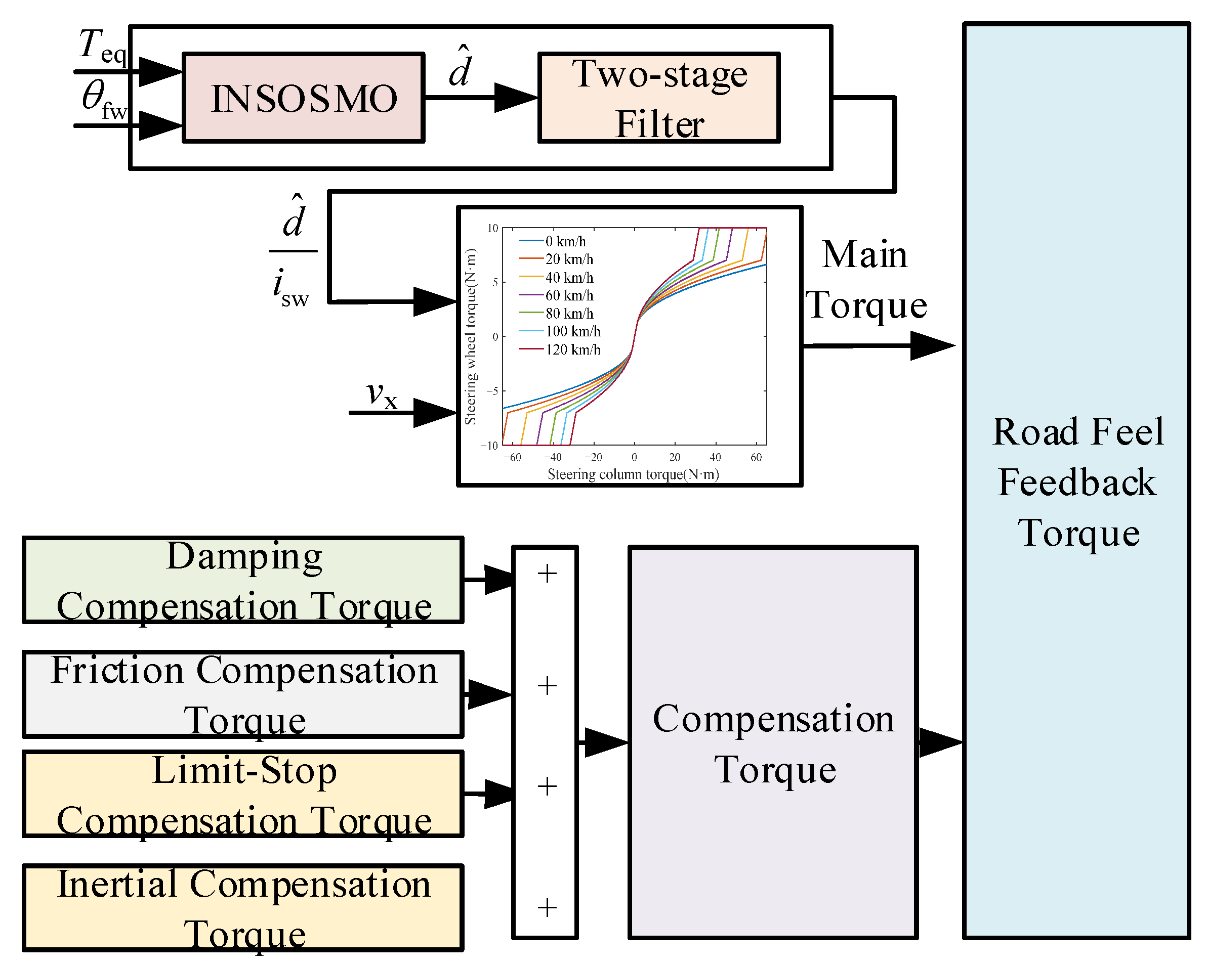
Road feel feedback torque refers to the reactive force perceived by the driver through the steering wheel during vehicle operation, representing a comprehensive manifestation of the vehicle’s overall state, road conditions, and the interactive dynamics of the steering system. The designed road feel feedback torque model consists of two components: the main torque and the compensation torque, as illustrated in Figure 4. Among them, the main road feel torque is designed based on system disturbance torque d, observed by the INSOSMO and further processed through a two-stage filter.

4.1. Design of the Two-Stage Filter

The filtering aims to reduce road vibration interference while preserving essential road information for driver perception. A two-order filter combining STKF and a first-order low-pass filter is designed.

(1)

Design of the strong tracking Kalman filter

The Kalman filter (KF) algorithm is an optimal regression data processing algorithm; in order to make the traditional KF better match the complex system, the KF algorithm is combined with the strong tracking filtering algorithm (STFA), and the STKF is designed to carry out the first level of filtering of $\widehat{d}$. The traditional KF algorithm can be divided into two modules of prediction and update, and its formula is as follows:

Prediction module:

$$\left\{\begin{array}{c}{\widehat{X}}_{k|k-1}=A_k{\widehat{X}}_{k-1}+B_k{U}_{K-1}\\ P_{k|k-1}=A_k{P}_{k-1}{A}_k^T+Q_{k-1}\end{array}\right.,$$

(45)

Update module:

$$\left\{\begin{array}{c}{\widehat{X}}_k={\widehat{X}}_{k|k-1}+K_k\left(Z_k-H_k{\widehat{X}}_{k|k-1}\right)\\ K_k={\displaystyle \raisebox{1ex}{$P_{k|k-1}{H}_k^T$}\!\left/ \!\raisebox{-1ex}{$\left(H_k{P}_{k|k-1}{H}_k^T+R_k\right)$}\right.}\\ P_k=P_{k|k-1}-K_k{H}_k{P}_{k|k-1}\end{array}\right.,$$

(46)

where A_k is the system-state matrix at moment k; B_k is the system input matrix at moment k; H_k is the system output matrix at moment k; P_k is the error covariance matrix at moment k; K_k is the Kalman filtering gain matrix at moment k; and Q_k and R_k are the covariance matrices of the system noise and measurement noise at moment k.

The STKF algorithm introduces a fading factor during the update of the error covariance matrix [26], and the error covariance prediction process with the inclusion of the fading factor is expressed as follows:

$$P_{k|k-1}={\lambda }_k{A}_k{P}_{(k-1)}{A}_k^T+Q_{(k-1)},$$

(47)

$$\left\{\begin{array}{c}{\lambda }_k=\left\{\begin{array}{c}{\lambda }_{0,k},{\lambda }_{0,k}\ge 1\\ 1,{\lambda }_{0,k}<1\end{array}\right.\\ {\lambda }_{0,k}={\displaystyle \raisebox{1ex}{$T_{\mathrm{r}}(N_k)$}\!\left/ \!\raisebox{-1ex}{$T_{\mathrm{r}}(M_k)$}\right.}\\ N_k=V_k-H_k{Q}_{k-1}{H}_k^T-l{R}_k\\ M_k=H_k{A}_k{P}_{k-1}{A}_k^T{H}_k^T\end{array}\right.,$$

(48)

$$\left\{\begin{array}{c}{V}_k=\left\{\begin{array}{c}{d}_1{d}_1^T,k=1\\ {\displaystyle \frac{\rho V_{k-1}+d_k{d}_k^T}{1+\rho }},k\ge 2\end{array}\right.\\ d_k=Z_k-H_k{\widehat{X}}_{k|k-1}\end{array}\right.,$$

(49)

where V_k is the new interest covariance matrix; ρ is the forgetting factor, generally taken as 0.95; and l is the weakening factor. l ≥ 1 and takes 5.

(2)

Design of a first-order low-pass filter

A first-order low-pass filter can effectively isolate high-frequency signals, with the basic formula being

$$Y(n)=pX(n)+(1-p)Y(n-1),$$

(50)

$$p={\displaystyle \frac{T}{T+0.5\pi fc}},$$

(51)

where p is the filter coefficient; T is the sampling period, which takes 0.001; fc is the cutoff frequency; X(n) is the current sampling value; and Y(n − 1) is the previous filter output value.

In the existing research, Reference [27] analyzes steering feedback torque from a frequency-domain perspective. The findings indicate that the vehicle motion state-dependent feedback torque components are primarily concentrated below 10 Hz. Therefore, the parameter p is designed to be 0.0591. Consequently, a first-order low-pass filter is superimposed on the STKF to design the two-stage filter that filters out high-frequency signals and smooths $\widehat{d}$, thereby enhancing driving feel.

4.2. Design of Road Feel Feedback Torque

4.2.1. Design of Main Road Feel Torque

The system aligning the torque of the tires after the action of the steering system transmission ratio, when transferred to the steering column, is reduced to T_z/i_sw, which can be expressed as the steering column torque T_col. The steering column torque T_col can be obtained by the following equation:

$$T_{\mathrm{col}}={\displaystyle \frac{\widehat{d}}{i_{sw}}},$$

(52)

To provide drivers with an easily adaptable road feel, the source of the road feel is analyzed using a column-type electric power steering system. Based on the curved power assist characteristic curve, the assist torque is designed to guarantee the lightness of the planned road feel torque. The curved power assist characteristic curve introduced for the EPS system is illustrated in Figure 5.

In addition, an analysis of the steering system reveals that T_col is equated to the sum of the assist torque T_assist and the steering wheel torque T_h. Therefore, based on this mathematical relationship, the steering column torque can be used to inversely obtain the desired steering wheel torque [6]. MATLAB’s finverse function can be employed to obtain its mathematical inverse function, which expresses the steering wheel torque. The resulting steering wheel torque curve is illustrated in Figure 6 and is expressed by Equation (53), as follows:

$$T_{\mathrm{main}}=f(T_{\mathrm{col}},v),$$

(53)

where T_main is the main road feel torque.

4.2.2. Design of the Compensation Torque

The main road feel torque can meet basic steering requirements. However, as the SBW system eliminates certain mechanical components, the driver cannot directly perceive information such as inertia, damping, and friction torque, which would normally be generated by these mechanical parts. Therefore, to more realistically simulate the road feel experience during actual driving, it is necessary to design compensation torque to restore these missing mechanical characteristics [12,13]. Additionally, since the SBW system lacks corresponding mechanical structures to alert drivers when the steering wheel’s rotation angle reaches its physical limit, it is necessary to design a corresponding limit-stop compensation torque to notify the driver when the steering wheel approaches its virtual limit position.

The final road feel feedback torque T_roadfeel is formulated as

$$T_{\mathrm{roadfeel}}=T_{\mathrm{main}}+T_{\mathrm{ine}}+T_{\mathrm{fric}}+T_{\mathrm{dam}}+T_{\mathrm{limit}},$$

(54)

where

$$\left\{\begin{array}{l}{T}_{\mathrm{ine}}=k_{\mathrm{ine}}{\ddot{\theta }}_{\mathrm{sw}}\\ T_{\mathrm{fric}}=k_{\mathrm{fric}}\tan \mathrm{h}\left({\rho }_1{\dot{\theta }}_{\mathrm{sw}}\right)\\ T_{\mathrm{dam}}=\left\{\begin{array}{c}0,v\le v_0\\ k_{\mathrm{dam}}(v-v_0){\dot{\theta }}_{\mathrm{sw}},v>v_0\end{array}\right.\\ T_{\mathrm{limit}}=\left\{\begin{array}{c}{k}_{\mathrm{limit}}\left(\left|{\theta }_{\mathrm{sw}}\right|-{\theta }_{\mathrm{limit}}\right),\left|{\theta }_{\mathrm{sw}}\right|>{\theta }_{\mathrm{limit}}\\ 0,\left|{\theta }_{\mathrm{sw}}\right|\le {\theta }_{\mathrm{limit}}\end{array}\right.\end{array}\right.,$$

(55)

where T_ine is the inertial compensation torque; k_ine is the inertial compensation torque coefficient; T_fric is the friction compensation torque; k_fric is the friction compensation torque coefficient; ρ₁ is the gradient coefficient of the friction compensation torque; T_dam is the damping compensation torque; k_dam is the damping compensation torque coefficient; v₀ is the threshold vehicle speed; T_limit is the limit-stop compensation torque; k_limit is the limit-stop compensation torque coefficient; and θ_limit is the steering wheel maximum rotation angle.

5. Steering Wheel Active Return Control Strategy

5.1. Driving Intent Judgment

To avoid confusion with traditional steering systems, the action of the steering wheel returning to its original position after the driver releases the steering wheel is called “return”, while the operation in which the steering wheel is not released by the driver is called “steering”. Driver driving intention judgment can be expressed as

$$\left\{\begin{array}{c}{\theta }_{\mathrm{sw}}{\dot{\theta }}_{\mathrm{sw}}\ge 0\&\&\left|{\theta }_{\mathrm{sw}}\right|>\mathsf{\Delta }{\theta }_{\mathrm{sw}},\mathrm{steering}\\ {\theta }_{\mathrm{sw}}{\dot{\theta }}_{\mathrm{sw}}<0\&\&\left|{\theta }_{\mathrm{sw}}\right|>\mathsf{\Delta }{\theta }_{\mathrm{sw}},\mathrm{return}\end{array}\right.\hspace{1em},$$

(56)

where $∆{\theta }_{\mathrm{s}\mathrm{w}}$ is the steering wheel dead zone angle.

5.2. Design of the Steering Wheel Active Return Controller

To enhance the steering wheel’s active return performance and prevent insufficient low-speed return or high-speed return overshoot, we designed an active return controller. The difference between the actual steering wheel angle and the desired angle is selected as the input, while the return torque from the road feel motor serves as the control output. Considering that the BSSMC algorithm is well suited for uncertain nonlinear systems that can be state-linearized or possess strict feedback parameter structures [28], this algorithm is adopted to design the steering wheel active return strategy. Equation (6) shows a dynamic analysis of the steering wheel subsystem during the return process, where its formula is as follows:

$$G_{\mathrm{m}}{T}_{\mathrm{return}}=J_{\mathrm{eq}1}{\ddot{\theta }}_{\mathrm{sw}}+B_{\mathrm{eq}1}{\dot{\theta }}_{\mathrm{sw}}+d_2,$$

(57)

where T_return is the steering wheel return torque; J_eq1 is the equivalent moment of inertia between the feedback motor and the steering wheel; B_eq1 is the equivalent damping coefficient between the feedback motor and the steering wheel; d₂ is the system disturbance; and $\left|d_2\right|\le D_2$, in the subsequent simulations, is set as a sine function with an amplitude of 0.5 N·m and a period of 5 s.

Let $x={[\begin{array}{cc}{x}_1& x_2\end{array}]}^{\mathrm{T}}={\left[\begin{array}{cc}{\theta }_{\mathrm{sw}}& {\dot{\theta }}_{\mathrm{sw}}\end{array}\right]}^{\mathrm{T}}$ and u = G_mT_return. From Equation (57), the state-space equation is derived as follows:

$$\left\{\begin{array}{l}{\dot{x}}_1=x_2\\ {\dot{x}}_2={\displaystyle \frac{1}{J_{\mathrm{eq}1}}}u-{\displaystyle \frac{B_{\mathrm{eq}1}}{J_{\mathrm{eq}1}}}{x}_2-{\displaystyle \frac{1}{J_{\mathrm{eq}1}}}{d}_2\end{array}\right.,$$

(58)

where

$$\left\{\begin{array}{l}{J}_{\mathrm{eq}1}=J_{\mathrm{sw}}+{G_{\mathrm{m}}}^2{J}_{\mathrm{f}}\\ B_{\mathrm{eq}1}=B_{\mathrm{sw}}+{G_{\mathrm{m}}}^2{B}_{\mathrm{f}}\\ d_2=\mathsf{\Delta }{J}_{\mathrm{eq}1}{\dot{x}}_2+\mathsf{\Delta }{B}_{\mathrm{eq}1}{x}_2+T_{\mathrm{fh}}+G_{\mathrm{m}}{T}_{\mathrm{ff}}\end{array}\right.,$$

(59)

Define the angular error e₁ as

$$e_1=x_1-x_{\mathrm{d}}={\theta }_{\mathrm{sw}}-0,$$

(60)

Then,

$${\dot{e}}_1={\dot{x}}_1-{\dot{x}}_{\mathrm{d}}=x_2-0,$$

(61)

The steps for the design of the backstepping sliding mode control algorithm are as follows:

Step 1: Define the Lyapunov function:

$$V_3={\displaystyle \frac{1}{2}}{e}_1^2,$$

(62)

Then,

$${\dot{V}}_3=e_1{\dot{e}}_1=e_1(x_2-0),$$

(63)

Take $x_2=-c_1{e}_1+e_2$, where c₁ > 0 and e₂ is the virtual control quantity, i.e., $e_2=x_2+c_1{e}_1$.

Then,

$${\dot{V}}_3=-c_1{e}_1^2+e_1{e}_2,$$

(64)

If e₂ = 0, then ${\dot{V}}_1\le 0$ is satisfied, and the next design step is required.

Step 2: Define the sliding mode surface as $s_1=e_2+{\lambda }_1{e}_1,{\lambda }_1>0$ in conjunction with the sliding mode variable structure control and define the Lyapunov function:

$$V_4=V_3+{\displaystyle \frac{1}{2}}{s}_1^2,$$

(65)

Then,

$${\dot{V}}_4={\dot{V}}_3+s_1{\dot{s}}_1=-c_1{e}_1^2+e_1{e}_2+s_1\left(c_1{\dot{e}}_1+{\displaystyle \frac{u}{J_{\mathrm{eq}1}}}-{\displaystyle \frac{d_2}{J_{\mathrm{eq}1}}}-{\displaystyle \frac{B_{\mathrm{eq}1}}{J_{\mathrm{eq}1}}}{x}_2+{\lambda }_1{\dot{e}}_1\right),$$

(66)

To satisfy ${\dot{V}}_2\le 0$, the controller is designed:

$$u=J_{\mathrm{eq}1}(-c_1{\dot{e}}_1-{\lambda }_1{\dot{e}}_1-h(s_1+k_3\mathrm{sign}\left(s_1\right)))+d_2+B_{\mathrm{eq}1}{x}_2,$$

(67)

where k is a constant.

In addition, an extended state observer is designed to observe the system disturbance d₂.

$$\left\{\begin{array}{c}{\dot{\widehat{x}}}_1={\widehat{x}}_2+l_1(x_1-{\widehat{x}}_1)\\ {\dot{\widehat{x}}}_2={\displaystyle \frac{u-{\widehat{d}}_2}{J_{\mathrm{eq}1}}}-{\displaystyle \frac{B_{\mathrm{eq}1}}{J_{\mathrm{eq}1}}}{\widehat{x}}_2+l_2(x_1-{\widehat{x}}_1)\\ {\dot{\widehat{d}}}_2=l_3(x_1-{\widehat{x}}_1)\end{array}\right.,$$

(68)

where l₁, l₂, and l₃ are the observer gain coefficients, respectively.

Therefore, Equation (67) can be rewritten as

$$u_2=J_{\mathrm{eq}1}\left(-c_1{\dot{e}}_1-{\lambda }_1{\dot{e}}_1-h(s_1+k_3\mathrm{sign}\left(s_1\right))\right)+{\widehat{d}}_2+B_{\mathrm{eq}1}{x}_2,$$

(69)

At this point, the design of the steering wheel return controller based on the backstepping sliding mode algorithm has been completed.

The stability of the algorithm is proved below:

Substituting Equation (69) into Equation (66), the sliding mode gain hk₃ must satisfy hk₃ > ϵ + D₂, where ϵ is the upper bound of the ESO estimation error:

$$\begin{array}{l}{\dot{V}}_4=-c_1{e}_1^2+e_1{e}_2-h{s}_1^2-h{k}_3\left|s_1\right|+{\displaystyle \frac{({\widehat{d}}_2-d_2)s_1}{J_{\mathrm{eq}1}}}\\ \le -c_1{e}_1^2+e_1{e}_2-h{s}_1^2-h{k}_3\left|s_1\right|+D_2\left|s_1\right|\\ \le -c_1{e}_1^2+e_1{e}_2-h{s}_1^2-ϵ\left|s_1\right|\end{array},$$

(70)

Let Q be equal to

$$Q=\left[\begin{array}{cc}{c}_1+h{\lambda }_1^2& h{\lambda }_1-{\displaystyle \frac{1}{2}}\\ h{\lambda }_1-{\displaystyle \frac{1}{2}}& h\end{array}\right],$$

(71)

because

$$\begin{array}{l}{e}^{\mathrm{T}}Qe=\left[\begin{array}{cc}{e}_1& e_2\end{array}\right]\left[\begin{array}{cc}{c}_1+h{\lambda }_1^2& h{\lambda }_1-{\displaystyle \frac{1}{2}}\\ h{\lambda }_1-{\displaystyle \frac{1}{2}}& h\end{array}\right]{\left[\begin{array}{cc}{e}_1& e_2\end{array}\right]}^{\mathrm{T}}\\ =c_1{e}_1^2-e_1{e}_2+h{\lambda }_1^2{e}_1^2+2h{\lambda }_1{e}_1{e}_2+h{e}_2^2\\ =c_1{e}_1^2-e_1{e}_2+h{s}_1^2\end{array},$$

(72)

Then, Q is guaranteed to be a positive definite matrix satisfying

$$\left|Q\right|=h(c_1+h{\lambda }_1^2)-{(h{\lambda }_1-{\displaystyle \frac{1}{2}})}^2=h(c_1+{\lambda }_1)-{\displaystyle \frac{1}{4}},$$

(73)

By appropriately selecting the values of h, c₁, and λ₁, matrix Q can be made positive and definite, thereby ensuring that ${\dot{V}}_2\le 0$. According to LaSalle’s invariance principle, the controller is guaranteed to achieve asymptotic convergence.

6. Simulation Verification

Based on the above, MATLAB/Simulink software is utilized to build the relevant simulation model, and joint simulation with CarSim is carried out for verification. The computer employed in this simulation is manufactured by Lenovo Group (Beijing, China), with the following detailed hardware configuration: the Intel Core i5-12400F processor (12th Gen, 2.50 GHz), the NVIDIA RTX 3050 graphics card, the 16 GB DDR4 RAM (3200 MHz), and the 512 GB PCIe 4.0 SSD. The operating system is 64-bit Windows 11, and the simulation software included CarSim 2019.0 and MATLAB R2021a.

6.1. Verification of Observer Performance

The parameters of the model are selected as follows: J_eq = 21.88 kg·m²; B_eq = 76.21 N·m·s/rad; K = 194.25; i_sw = 18.5; α = 0.3; p/q = 1.5; k = 20; ε = 10; G = −40.88; λ = 50; c = 0.9; n₁ = 50; n₂ = 50; k₁ = 28.9336; k₂ = 20; β₁ = 206.5169; β₂ = 139.81; β₃ = −7,504,840; k₄ = 70; ε₄ = 0.5; c₂ = 50; c₃ = 50; and system friction torque set to $T_{\mathrm{f}}=2.5\tanh (60{\dot{\theta }}_{\mathrm{fw}})$. Additionally, the backstepping control (BSC) algorithm is introduced as the steering angle tracking comparative algorithm. Furthermore, to demonstrate the superiority of the proposed INSOSMO, the SMO, ESO, and KFO [14] are added for comparison. The SSA fitness iteration curve is shown in Figure 7.

BSC:

$$u_3=J_{\mathrm{eq}}({\displaystyle \frac{B_{\mathrm{eq}}}{J_{\mathrm{eq}}}}{x}_2+{\displaystyle \frac{{\widehat{x}}_3}{J_{\mathrm{eq}}}}-c_2{\dot{z}}_1+{\ddot{z}}_{\mathrm{d}}-c_3{z}_2-z_1),$$

(74)

ESO:

$$\left\{\begin{array}{c}{\dot{\widehat{x}}}_1={\widehat{x}}_2+{\beta }_1\left(x_1-{\widehat{x}}_1\right)\\ {\dot{\widehat{x}}}_2=-{\displaystyle \frac{B_{\mathrm{eq}}{\widehat{x}}_2}{J_{\mathrm{eq}}}}-{\displaystyle \frac{\widehat{d}}{J_{\mathrm{eq}}}}+{\displaystyle \frac{u}{J_{\mathrm{eq}}}}+{\beta }_2\left(x_1-{\widehat{x}}_1\right)\\ \dot{\widehat{d}}={\beta }_3\left(x_1-{\widehat{x}}_1\right)\end{array}\right.,$$

(75)

SMO:

$$U_{\mathrm{SMO}}=-{\displaystyle \frac{k_4}{1+c}}s-{\displaystyle \frac{{\epsilon }_4}{1+c}}\mathrm{sign}(s),$$

(76)

First, the verification of the observer performance is conducted through both sinusoidal tests and the double-lane-change (DLC) test. For the sinusoidal test, the steering wheel angle input is set as a sine wave with an amplitude of 50 deg and a frequency varying from 0.2 Hz to 0.5 Hz within 20 s at a vehicle speed of 80 km/h. For the DLC test, the steering wheel angle input is set according to the standard DLC trajectory, with a vehicle speed of 60 km/h. In order to clarify the observation error of each observer, the MAE is introduced to represent the error under different tests. The MAE can be expressed as

$$\mathrm{MAE}={\displaystyle \frac{1}{n}}{\displaystyle \sum _{i=1}^n\left|\left(pv-av\right)\right|}$$

(77)

where n is the number of samples, pv is the predicted value, and av is the actual value.

The specific results are shown in

Table 1. MAE under different tests.

	Sinusoidal Test	Percentage Improvement	DLC Test	Percentage Improvement
INSOSMO	6.6582		1.7401
KFO	17.7638	62.5%	4.5581	61.8%
ESO	10.1953	34.7%	2.6285	33.8%
SMO	16.7061	60.1%	3.0605	43.1%

.

The simulation results are shown in Figure 8 and Figure 9.

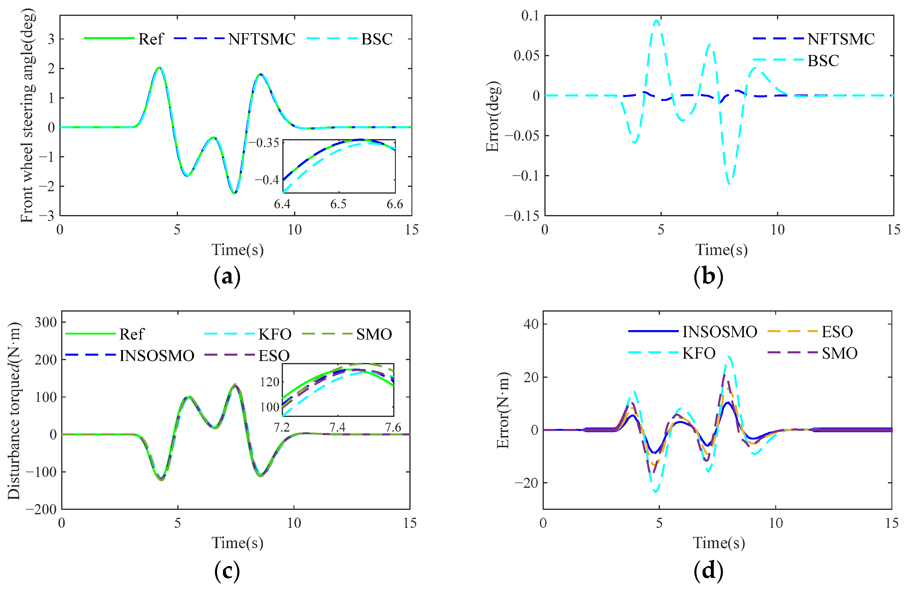
The sinusoidal test is conducted to simulate obstacle avoidance maneuvers in daily driving scenarios, where vehicles navigate through multiple obstacles via repeated left–right steering. The analysis of Figure 8a,b reveals that NFTSMC exhibits superior tracking accuracy compared to BSC. As the steering frequency increases, the tracking error of both control algorithms progressively rises, indicating that high-frequency steering induces larger errors. The maximum tracking error, attributed to system disturbance torque d, occurs at the peak steering angle. Specifically, NFTSMC achieves a peak error of 0.0503 deg, while BSC yields 0.1511 deg, representing a 66.7% reduction in tracking error. It is evident that NFTSMC demonstrates superior tracking accuracy and can more precisely respond to driver input commands. Consequently, the system disturbance torque d observed based on this method better aligns with the driver’s expectations, and the resulting road feel torque more accurately reflects road information under the driver’s intended operating conditions. The further analysis of Figure 8c,d demonstrates that the INSOSMO outperforms KFO, ESO, and SMO in observation accuracy, enabling precise feedforward compensation for the control algorithm. Additionally, as shown in Table 1, the observation performance of the INSOSMO is enhanced by 62.5%, 34.7%, and 60.1%, respectively.

The DLC test is conducted to simulate vehicle lane-switching behavior. The analysis of Figure 9a,b demonstrates that NFTSMC maintains significantly higher tracking accuracy than BSC. During the lane-change maneuver, tracking errors progressively increase for both algorithms, with peak errors occurring at approximately 7.6 s—0.0088 deg for NFTSMC versus 0.1105 deg for BSC—coinciding with the transition back to straight-line driving. Figure 9c,d reveal that the system disturbance torque d observation error also peaks at this critical phase, confirming its substantial impact on control precision. Furthermore, Table 1 shows that the observation performance of INSOSMO is enhanced by 61.8%, 33.8%, and 43.1%, respectively.

Consequently, the results demonstrate that NFTSMC maintains superior tracking accuracy; the system disturbance torque d directly degrades control precision; and the INSOSMO achieves precise disturbance estimation, laying the foundation for road feel feedback torque design.

6.2. Verification of Road Feel Feedback Torque

The performance evaluation of road feel feedback torque can be quantified based on the dynamic mapping relationship between lateral acceleration, steering wheel torque, and steering wheel angle. In high-speed driving conditions, where steering precision and stability are prioritized, the high-speed on-center handling test is typically employed to assess road feedback torque. Conversely, in low-speed driving conditions, where steering ease is the primary objective, the low-speed lemniscate test is commonly used for evaluation. Furthermore, to comprehensively validate the dynamic performance of the designed road feel feedback torque, the steering wheel torque filtering test and the steering angle limit test are incorporated alongside the high-speed on-center handling test and low-speed lemniscate test for more thorough verification. The parameters of the road feel torque are selected as follows: k_ine = 0.15 kg·m²; k_fric = 0.65 N·m·s/deg; ρ₁ = 60; k_dam = 0.03 kg·m/deg; v₀ = 30 km/h; k_limit = 0.65 N·m/deg; and θ_limit = 370 deg.

The lemniscate test: The lemniscate test evaluates steering wheel torque–angle characteristics across speeds, while validating compliance with low-speed steering effort requirements. In CarSim, the vehicle speed is set at 15 km/h to conduct a simulation test along a lemniscate path for one complete revolution, and the obtained simulation results are presented in Figure 10.

As analyzed in Figure 10, the work required by the driver to rotate the steering wheel during a low-speed lemniscate test is significantly less than that of the EPS system, while the average friction torque of the SBW system’s steering wheel is also smaller than that of the EPS system. Additionally, due to the presence of friction torque, when the steering wheel begins to rotate, the torque suddenly increases to 0.81 N·m. When the steering wheel angle is between 0 deg and 80 deg, the steering wheel torque gradient is relatively large. When the steering wheel rotation angle exceeds 80 deg, the steering wheel torque gradient starts to decrease. When the steering wheel angle reaches 321 deg, the steering wheel torque reaches its maximum value of 3.25 N·m. It can be seen that the designed road feel feedback torque can meet the lightness requirements under low-speed driving conditions.

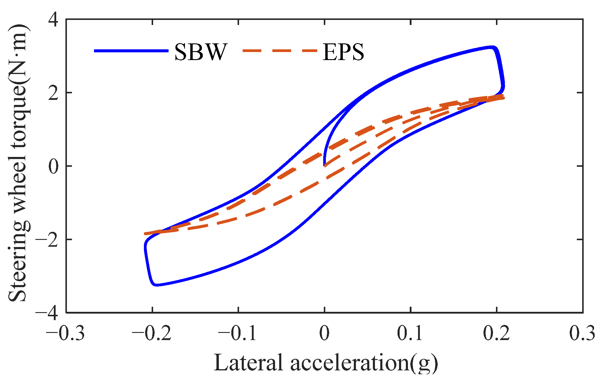
On-center handling test: The on-center handling test is used to evaluate the change in the steering wheel torque gradient of a vehicle at high speed. According to the ISO standard [29], set the vehicle speed to 100 km/h. Apply a sinusoidal steering wheel input with an amplitude of 12 deg and a period of 0.2 Hz, generating a maximum lateral acceleration of approximately 0.2 g . The resulting simulation data are presented in Figure 11.

Based on the analysis of Figure 11, the steering wheel torque of the SBW system at 0 g lateral acceleration is significantly greater than that of the EPS system, indicating that it possesses stronger system dry friction characteristics that can effectively prevent unintended vehicle lateral motion caused by driver misoperation. The torque gradient of the SBW system at 0 g is significantly greater than that of the EPS system, demonstrating clearer road feel during straight-line driving conditions, which helps drivers better perceive the steering wheel’s center position through road feel variations. At 0.1 g lateral acceleration, the SBW system’s steering wheel torque gradient is significantly greater than the EPS system’s, with the SBW system’s maximum torque being 3.17 N·m compared to the EPS system’s 1.82 N·m. This indicates that during high-speed steering maneuvers, the designed road feel feedback torque is clearer and more stable, meeting the design requirements for road feel feedback torque.

Steering wheel torque filtering test: To validate the effectiveness of the designed two-order filter, a sinusoidal steering wheel input with an amplitude of 40 deg and a frequency of 0.1 Hz is applied at a constant vehicle speed of 60 km/h. The observed system disturbance torque is then processed through the filter. The simulation results are presented in Figure 12.

The analysis of Figure 12 demonstrates that the two-stage filter effectively smooths the steering wheel torque while reducing force discontinuities, yet preserves essential road roughness information. This achieves the objective of improving driver steering feel.

Steering angle limit test: To verify the effectiveness of the designed limit-stop compensation torque, the steering wheel limit rotation angle is set to 360 deg, with the vehicle speed set to 10 km/h, steering wheel angle input set to a sinusoidal signal with an amplitude of 370 deg and a frequency of 1/60 Hz, and simulation time set to 60 s. The results are shown in Figure 13.

As can be analyzed from Figure 13, when the steering wheel angle exceeds 360 deg, the system triggers the limit-stop compensation torque mechanism, causing the steering wheel torque to rapidly increase to 5.78 N·m. At this point, if the driver continues to turn the steering wheel, they will experience significant resistance, which effectively alerts the driver that the steering wheel has reached its limit position.

6.3. Verification of the Steering Wheel Active Return Strategy

In order to verify the effectiveness of the designed steering wheel active return controller, the vehicle speed is set to 30 km/h and to 80 km/h, the driver inputs a constant torque to the steering wheel, and then the driver releases the steering wheel after 4 s to obtain the change curve of the steering wheel angle over time under the steering wheel active return controller designed. The simulation results are shown in Figure 14. The parameters of the ESO-BSSMO are selected as follows: J_eq1 = 4.30026 kg·m²; B_eq1 = 2.3169 N·m·s/rad; l₁ = 599.9462; l₂ = 119,970; l₃ = −312,000; k₃ = 2; c₁ = 70; λ₁ = 15; and h = 25.

Based on the analysis of Figure 14a,b, the designed driving intention judgment program can accurately determine the driver’s intention, where “0” represents the steering process and “1” represents the active return process. At the time of 4 s, when the driver releases the steering wheel, the steering wheel begins to return to the center. Without the inclusion of active return control, the steering wheel exhibits insufficient return during low-speed return and overshoot during high-speed return. The residual return angle at low speed is approximately 2.5 deg. Moreover, the rate of speed adjustment is too slow; the return overshoot at high speed is approximately 5.5 deg. However, with the addition of active return control, the steering wheel can effectively avoid these issues and improve the return performance of the SBW system. Furthermore, under low-speed return conditions, the steering wheel achieves recentering at 4.4 s, while at high-speed conditions, recentering is completed by 4.3 s.

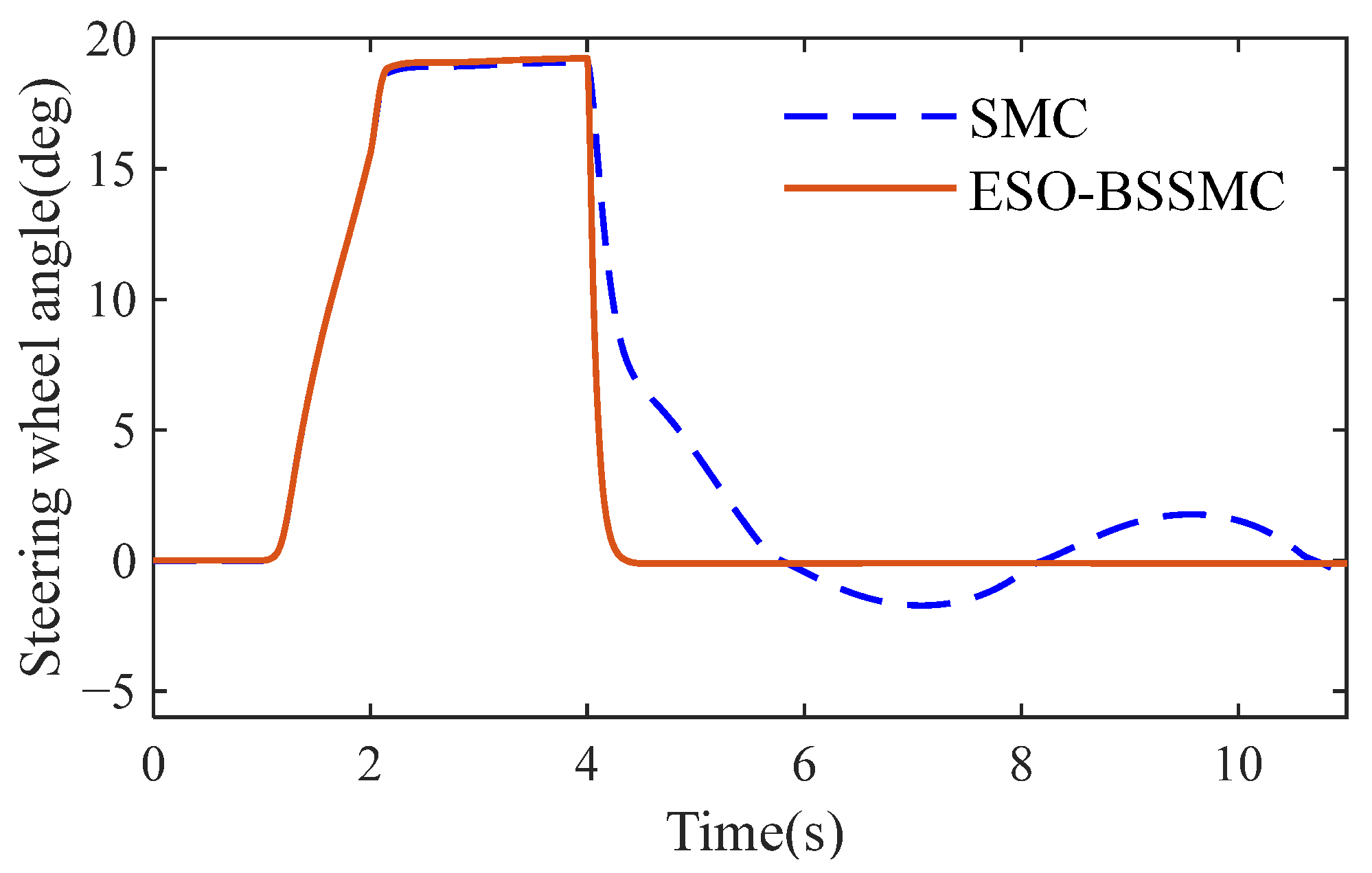
Additionally, a continuous disturbance torque is incorporated during the return process, and comparative analysis is conducted with a return controller (SMC) from the existing literature [11]. The simulation results are shown in Figure 15.

Based on the analysis of Figure 15, it can be seen that under the influence of the disturbance torque, it is difficult for SMC to achieve an accurate return-to-center of the steering wheel. In contrast, the controller designed in this study can realize accurate return-to-center of the steering wheel and possesses better robustness.

7. Conclusions

With the research objective of simulating the road feel of SBW systems, a dynamics model of an SBW system is established in MATLAB/Simulink. The study focuses on the planning of road feel feedback torque and the active return control of the steering wheel. The main results are summarized below:

(1)

This study develops a high-precision INSOSMO-based method for road feel feedback torque planning through observation of system disturbance torque. Firstly, an NFTSMC is designed to achieve precise angle tracking control for the SBW system. Meanwhile, an INSOSMO is developed for the real-time estimation of system disturbance torque . Secondly, a two-stage filter is designed to process the observed system disturbance torque through filtering, which is then combined with the assist torque to generate the main road feel torque. Finally, the main road feel torque is optimized and adjusted by designing a compensation torque, and the road feel feedback torque is generated by superimposing the main torque and the compensation torque. The simulation results indicate that NFTSMC exhibits higher tracking accuracy compared to BSC. The INSOSMO demonstrates superior observation accuracy; compared with KFO, ESO, and SMO, the observation performance of the INSOSMO is enhanced by 62.5%, 34.7%, and 60.1%, respectively, in the sinusoidal test, and by 61.8%, 33.8%, and 43.1%, respectively, in the DLC test. The designed road feel feedback torque demonstrates superior characteristics compared to the torque in the EPS system, being lighter during low-speed steering and heavier during high-speed steering.

(2)

In the research on the active return control of the steering wheel, a return controller incorporating system nonlinear disturbances is designed. The BSSMC algorithm is adopted to design an active return controller for steering wheels. Additionally, an ESO is employed to observe the nonlinear disturbances in the steering wheel subsystem , which are then used to compensate for the controller. The simulation results indicate that the designed steering wheel return controller can improve the vehicle’s return performance, effectively avoid insufficient return and overshoot phenomena, and demonstrate good robustness.

However, this study does not account for the impact of sensor signal noise on observer performance. Future research should rigorously investigate the influence of sensor noise on the observer’s robustness and estimation accuracy, and experimental validation of the developed algorithm’s effectiveness through real-vehicle testing.

References

1. He, L.; Huang, C.; Xu, Z.; Li, S.; Guo, C.; Shi, Q. A model-tuned predictive backstepping control approach for angle following of steer-by-wire. IEEE Trans. Intell. Transp. Syst. 2024, 25, 8053–8062. [Google Scholar] [CrossRef]
2. Wu, J.; Zhang, J.; Nie, B.; Liu, Y.; He, X. Adaptive control of PMSM servo system for steering-by-wire system with disturbances observation. IEEE Trans. Transp. Electrif. 2022, 8, 2015–2028. [Google Scholar] [CrossRef]
3. Wu, X.; Li, W. Variable steering ratio control of steer-by-wire vehicle to improve handling performance. Proc. Inst. Mech. Eng. Part D J. Automob. Eng. 2020, 234, 774–782. [Google Scholar] [CrossRef]
4. Xu, K.; Zhou, X.; Zhao, W.; Wang, C.; Luan, Z.; Liang, W. Performance-guaranteed adaptive switching fault-tolerant control of steer-by-wire system considering actuator fault and load disturbance. IEEE Trans. Transp. Electrif. 2024, 10, 8513–8527. [Google Scholar] [CrossRef]
5. Han, J.; Zhao, J.; Zhu, B.; Song, D. Adaptive steering torque coupling framework considering conflict resolution for human-machine shared driving. IEEE Trans. Intell. Transp. Syst. 2022, 23, 10983–10995. [Google Scholar] [CrossRef]
6. Yu, L.; Hu, Z.; Cai, Y.; Hou, Z.; Shi, Y.; Wu, B.; Tian, M. Road feel simulation method with rack force observer for intelligent vehicle steer-by-wire system. Int. J. Automot. Technol. 2025, 26, 491–504. [Google Scholar] [CrossRef]
7. Liang, X.; Zhao, L.; Wang, Q.; Chen, W.; Xia, G.; Hu, J.; Jiang, P. A novel steering-by-wire system with road sense adaptive friction compensation. Mech. Syst. Signal Process. 2022, 169, 108741. [Google Scholar] [CrossRef]
8. Choi, H.; Choi, S. Design of the steering feedback controller of a steer-by-wire system using admittance model. Int. J. Automot. Technol. 2024, 25, 565–574. [Google Scholar] [CrossRef]
9. Xie, Y.; Zhao, L.; Chen, W.; Liu, Y. Road feel and return control on low friction coefficient road for steer-by-wire vehicles. J. Mech. Eng. 2019, 55, 148–158. [Google Scholar]
10. Zhao, W.; Zhang, H.; Zou, S.; Xu, S.; Liu, C. Overview of vehicle steer-by-wire system control technologies. J. Automot. Saf. Energy 2021, 12, 18–34. [Google Scholar]
11. Zhao, H.; Li, F.; Wu, Y.; Liao, C. Road feel simulation and active return control strategy of steer-by-wire system. Adv. Technol. Electr. Eng. Energy 2020, 39, 64–72. [Google Scholar]
12. Shi, G.; Liu, T.; Wang, S.; Guo, C.; Liu, Y. High authenticity steering feel control strategy for Steer-by-Wire system based on terminal sliding mode rack force observer. Proc. Inst. Mech. Eng. Part D-J. Automob. Eng. 2024, 09544070241233859. [Google Scholar] [CrossRef]
13. Su, C.; Li, H.; Qiao, B.; Wu, X. Personalized steering feel design for Steer-by-Wire systems based on the rack force estimation. Int. J. Automot. Technol. 2023, 24, 1151–1161. [Google Scholar] [CrossRef]
14. Zheng, H.; Zong, C.; Wang, X. Road feel design for vehicle steer-by-wire system. Trans. Chin. Soc. Agric. Mach. 2011, 42, 18–22. [Google Scholar]
15. Liu, Y.; Wang, X.; Zhang, G.; Yuan, Q.; Chen, Z.; Li, L. Road sense construction for steer-by-wire system: Data-driven feedback torque design and friction compensated explicit model predictive control. IEEE Trans. Transp. Electrif. 2024, 10, 9918–9930. [Google Scholar] [CrossRef]
16. Zhao, R.; Deng, W.; Huang, K.; Nan, J.; Zheng, B. An innovative generalization method for data-driven models of steering feedback torque. Proc. Inst. Mech. Eng. Part D-J. Automob. Eng. 2023, 27, 2775–2785. [Google Scholar] [CrossRef]
17. Chugh, T.; Bruzelius, F.; Klomp, M.; Jacobson, B. Steering feedback transparency using rack force observer. IEEE/ASME Trans. Mechatron. 2022, 27, 3853–3864. [Google Scholar] [CrossRef]
18. Wu, X.; Zhang, M.; Xu, M. Active tracking control for steer-by-wire system with disturbance observer. IEEE Trans. Veh. Technol. 2019, 68, 5483–5493. [Google Scholar] [CrossRef]
19. Li, Z.; Shi, S.; Zhang, C. Active return control strategy of electric power steering system based on disturbance observer. J. Eng. Sci. Technol. Rev. 2018, 11, 61–69. [Google Scholar] [CrossRef]
20. Chen, H.; Zhang, L.; Gao, B. Active return control of EPS based on model reference fuzzy adaptive control. In Proceedings of the 2011 IEEE International Conference on Mechatronics, Istanbul, Turkey, 13–15 April 2011; pp. 194–199. [Google Scholar]
21. Huang, C.; Naghdy, F.; Du, H.; Huang, H. Fault tolerant steer-by-wire systems: An overview. Ann. Rev. Control 2019, 47, 98–111. [Google Scholar] [CrossRef]
22. Lee, J.; Yi, K.; Lee, D.; Jang, B.; Kim, M.; Hwang, S. Haptic control of Steer-by-Wire systems for tracking of target steering feedback torque. Proc. Inst. Mech. Eng. Part D-J. Automob. Eng. 2020, 234, 1389–1401. [Google Scholar] [CrossRef]
23. Ma, B.; Wang, Y. Adaptive output feedback control of steer-by-wire systems with event-triggered communication. IEEE/ASME Trans. Mechatron. 2021, 26, 1968–1979. [Google Scholar] [CrossRef]
24. Liu, Y.; Shi, Z.; Fu, B.; Xu, H.H. Radar error correction method based on improved sparrow search algorithm. Appl. Sci. 2024, 14, 3714. [Google Scholar] [CrossRef]
25. Moreno, J.A.; Osorio, M. Strict lyapunov functions for the super-twisting algorithm. IEEE Trans. Autom. Control 2012, 57, 1035–1040. [Google Scholar] [CrossRef]
26. Zhang, H.; Xie, J.; Ge, J.; Zong, B. Adaptive strong tracking square-root cubature kalman filter for maneuvering aircraft tracking. IEEE Access 2018, 6, 10052–10061. [Google Scholar] [CrossRef]
27. Groll, M.V.; Mueller, S.; Meister, T.; Rudolf, T. Disturbance compensation with a torque controllable steering system. Veh. Syst. Dyn. 2006, 44, 327–338. [Google Scholar] [CrossRef]
28. He, L.; Guo, C.; Xu, Z.; Huang, C.; Wei, Y.; Shi, Q. Particle-swarm backstepping control for angle tracking of electric motor steer-by-wire system. IEEE Trans. Transp. Electrif. 2023, 9, 2038–2047. [Google Scholar] [CrossRef]
29. ISO 13674-1:2010; Road Vehicles—Test Methods for the Quantification of On-centre Handling—Part 1: Weave Test. International Organization for Standardization: Geneva, Switzerland, 2010.
Figure 1. Schematic structure of SBW system.
Wevj 16 00294 g001
Figure 2. Block diagram of the observer principle.
Wevj 16 00294 g002
Figure 3. Flowchart of the SSA.
Wevj 16 00294 g003
Figure 4. Road feel feedback torque architecture.
Wevj 16 00294 g004
Figure 5. The curved power assist characteristic curve.
Wevj 16 00294 g005
Figure 6. Steering wheel torque curve.
Wevj 16 00294 g006
Figure 7. The fitness iteration curve.
Wevj 16 00294 g007
Figure 8. Response curves during the sinusoidal test: (a) steering angle tracking curve; (b) steering angle tracking error; (c) observed system disturbance torque d curve; (d) observation error of system disturbance torque d.
Wevj 16 00294 g008
Figure 9. Response curves during the DLC test: (a) steering angle tracking curve; (b) steering angle tracking error; (c) observed system disturbance torque d curve; (d) observation error of system disturbance torque d.
Wevj 16 00294 g009
Figure 10. Steering wheel angle–torque characteristic curve at a speed of 15 km/h.
Wevj 16 00294 g010
Figure 11. Lateral acceleration–steering wheel torque characteristic curve at a speed of 100 km/h.
Wevj 16 00294 g011
Figure 12. Steering wheel torque variation curve in steering wheel filtering test.
Wevj 16 00294 g012
Figure 13. Steering wheel angle–torque characteristic curve in steering angle limit test.
Wevj 16 00294 g013
Figure 14. Steering wheel active return test: (a) comparison of steering wheel active return control effect at vehicle speed of 30 km/h; (b) comparison of steering wheel active return control effect at vehicle speed of 80 km/h.
Wevj 16 00294 g014
Figure 15. Results of disturbance torque interference test.
Wevj 16 00294 g015