Trajectory Tracking in Autonomous Driving Based on Improved hp Adaptive Pseudospectral Method

Abstract

Intelligent driving technology can effectively improve transportation efficiency and vehicle safety and has become a development trend in automotive technology. As one of the core technologies of autonomous driving, path tracking control is directly related to the driving safety and comfort of vehicles and therefore has become a key research area of autonomous driving technology. In order to improve the reliability and control accuracy of path tracking algorithms, this paper proposed a path tracking control method based on the Gaussian pseudospectral method. Firstly, a vehicle motion model was constructed, and then an optimal trajectory solving method based on the hp adaptive pseudospectral method was proposed. The optimal trajectory control problem with differential constraints was transformed into an algebraic constrained nonlinear programming problem and solved using the sequential quadratic programming and compared with traditional control methods. The simulation results show that the tracking error of the lateral distance under the condition of $\mu =0.8$ is smaller than that of $\mu =0.4$. At the same time, the tracking error of the lateral distance under the condition of u = 30 km/h is smaller than that of u = 90 km/h. The optimal path tracking control using the improved hp adaptive pseudospectral method has higher accuracy and better control effect compared to traditional control algorithms. Finally, virtual and real vehicle tests were conducted to verify the effectiveness and accuracy of the improved hp adaptive trajectory control algorithm.

1. Introduction

The safety of intelligent vehicles is closely related to the nonlinear behavior of vehicle dynamics. Due to the inherent nonlinearity of the vehicle system during operation, factors such as changes in vehicle speed, uncertainty in tire cornering stiffness, and uncertainty in driver steering have a significant impact on the lateral stability of the vehicle under various operating conditions. The path tracking and lateral motion control of vehicles are important research topics in intelligent vehicles. Path tracking control is a key technology for intelligent vehicles. However, under low adhesion and high-speed driving conditions, the accuracy of path tracking may decrease, and accidents may occur due to skidding. Therefore, intelligent vehicles have great research value by comprehensively considering tracking accuracy and vehicle handling stability control. With the increasing demand for safe, comfortable, energy-saving, and time-saving transportation services, many domestic and international automobile companies have researched intelligent driving vehicles. The purpose of trajectory tracking is to enable vehicles to travel accurately along planned routes, ensuring the accuracy of path tracking and the stability of vehicle handling during the tracking process. It is a key technology for intelligent vehicle trajectory tracking [1,2,3].

The problem of vehicle lane changing has been widely studied. A brief review is presented below.

Zhao et al. applied sliding mode control to the active steering controller of the vehicle front wheels, enabling real-time correction of the front wheel steering angle [4]. They also designed a vehicle stability controller using the MPC method, achieving smooth and fast switching between various controllers. Most scholars had conducted research on path tracking control that considered stability, providing great potential for the integrated control of AFS and DYC. Compared to simple integrated control, the coordinated control structure could fully consider the interaction between various subsystems, and had the advantages of high flexibility, good fault tolerance, and high control accuracy [5]. In reference [6], the real-time path of the preceding vehicle was obtained based on V2V communication, and a smooth target path of the following vehicle was obtained using a cubic uniform B-spline curve interpolation method. In reference [7], based on the speed of the preceding vehicle, the distance between the ego vehicle and the preceding vehicle, and the recorded path of the preceding vehicle, a curvature continuous reference trajectory was generated using a quadratic programming method. This method ignored the road environment structure and considered the dynamic and kinematic constraints of the self-driving vehicle, ensuring the feasibility and safety of the planned trajectory. Wei et al. designed a linear feed-forward and feedback controller constrained by queue stability to ensure a safe distance between vehicles. The proposed method had good tracking performance on straight roads or under conditions of constant road curvature, but it was difficult to apply to conditions of road curvature changes. This type of method could achieve stable tracking of the preceding vehicle, but it relied on absolutely accurate positioning information, making it difficult to apply in scenarios where the positioning signal was unstable or obstructed [8]. Liu et al. proposed a lateral queue control system considering the dynamic characteristics of vehicles, which included two lateral control strategies: simultaneous steering and sequential steering and achieved stable driving of the queue with variable speed in general road curvature scenarios. However, due to the fact that the following vehicle directly followed the preceding vehicle instead of following a circular path, once the sensor detected a different heading from the preceding vehicle, it would immediately control the following vehicle to turn, resulting in premature turning and ultimately leading to the phenomenon of “taking shortcuts”. Moreover, as the fleet size expanded and the distance between vehicles increased, the overall lateral following error of the fleet would continue to accumulate [9]. Chen et al. fabricated a variable stiffness connecting rod in the workshop, and the flexibility of each slice of the connecting rod varied with the curvature of the road. The proposed method alleviated the phenomenon of internal cutting to a certain extent [10]. Bayuwindra et al. proposed a longitudinal and transverse system control method for tricycle queues. When the convoy passed corners, the cutting behavior was alleviated by extending the tracking points of the following vehicles, achieving small error tracking of the convoy under constant road curvature [11]. Duan et al. researched the on-center handling performance of light-duty trucks [12]. Park et al. obtained the steering wheel angle based on a PID controller and designed dead zone compensation to improve path tracking performance and stability [13]. Kigezi et al. proposed a vibration-free sliding mode controller using only conventional sliding surfaces for the path tracking problem of non-holonomic wheeled mobile robots [14]. Li et al. introduced a novel algorithm for vehicle path tracking control [15]. Wang et al. designed steering controllers using different fuzzy inference rules to handle both simple and complex path tracking problems [16]. Ren et al. proposed a path planning method based on virtual potential field theory and an autonomous vehicle path tracking framework based on multi-constraint MPC [17]. In order to solve the bottleneck problem of track slippage and body sinking of the tracked mining vehicle in the traditional deep-sea mining system, Chen et al. proposed a novel ROV-based deep-sea mining system [18]. Li et al. proposed an improved prediction method for electric vehicle charging for transportation system operations [19]. Cai et al. considered the limited applicability of a single controller under composite working conditions and designed a multi-controller switching scheduling logic based on working condition recognition [20]. Different controllers were selected for trajectory tracking under different vehicle states and working conditions. The proposed method could achieve accurate tracking at both high and low speeds, but due to the existence of hierarchical control, the computational burden increased. Salzmann et al. dealt with an accurate, robust, and efficient optimization method for time-optimal path planning on circular tracks [21]. Croce et al. proposed a bi-level procedure to calibrate the whole parameters of traffic flow models and energy consumption laws [22]. Liu et al. proposed a hp adaptive pseudospectral method for solving the vehicle path tracking problem [23].

In the above studies, the important parameter of path tracking is often set to a constant value, which often leads to the inability of the vehicle to make changes according to the actual complex driving conditions during actual tracking, thus failing to meet the accuracy of path tracking. The hp adaptive pseudospectral method is developed from the general pseudospectral method. On the one hand, it combines the advantages of the general pseudospectral method, and on the other hand, its discretization process is similar to that of the global pseudospectral method. Therefore, this article applies this method to solve the problem of path tracking in autonomous driving.

On the basis of Reference [23], this article improves the hp adaptive error evaluation criteria and the estimation of the polynomial order as well as the hp adaptive iteration strategy to form an improved hp adaptive pseudospectral method and applies it to the problem of vehicle path tracking. This method draws on the advantages of the global pseudospectral method and grid subdivision method, and has a more reasonable distribution of points, thereby improving the optimization efficiency of the algorithm.

2. Mathematical Model of Vehicle Path Tracking Problem

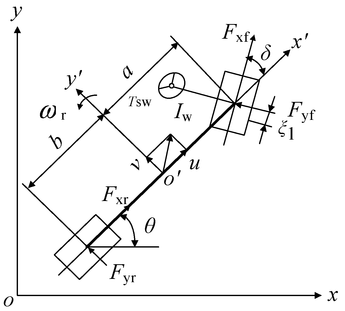
2.1. Mathematical Model of Vehicle

A nonlinear 4-DOF vehicle model shown in Figure 1 is used to describe the vehicle path tracking problem.

In the state space form, it is [1]

$$\left\{\begin{array}{l}\dot{v}=-u\omega +{\displaystyle \frac{F_{yf}\cos \delta +F_{yr}+F_{xf}\sin \delta }{m}}\\ {\dot{\omega }}_r={\displaystyle \frac{a{F}_{yf}\cos \delta -b{F}_{yr}+a{F}_{xf}\sin \delta }{I_z}}\\ \dot{u}=v\omega +{\displaystyle \frac{F_{xf}\cos \delta -F_{yf}\sin \delta +F_{xr}-F_f-F_w}{m}}\\ \dot{\delta }=p\\ \dot{p}=-{\displaystyle \frac{k_1{\xi }_1}{I_{w}u}}v-{\displaystyle \frac{k_1{\xi }_{1}a}{I_{w}u}}\omega +{\displaystyle \frac{(k_1{\xi }_1-k_w)}{I_w}}\delta -{\displaystyle \frac{c_w}{I_w}}p+{\displaystyle \frac{T_{sw}i}{I_w}}\end{array}\right..$$

(1)

The state variable is $\mathit{x}(t)=[u(t),v(t),\omega (t),x(t),y(t)]$ and the control variable is $\mathit{z}(t)=[\delta ]$. $v(t)$ and $u(t)$ can be measured using Steering torque/angle tester; $\delta$ can be measured using GPSSD-20 Speed measuring instrument. Then, Equation (2) can be obtained by simplifying Equation (1):

$$\dot{\mathit{x}}=f[\mathit{x}(t),\mathit{z}(t)].$$

(2)

2.2. Optimal Control Object of Path Tracking Problem

The minimum tracking error to complete the path tracking process is determined as the control object.

The cost function is [1]

$$J(\mathit{z})={\displaystyle {\int }_{t_0}^{t_f}\left({\left(\frac{y-y_d}{\widehat{E}}\right)}^2+{\left(\frac{\mathit{z}}{{\widehat{T}}_{sw}}\right)}^2\right)}dt={\displaystyle {\int }_{t_0}^{t_f}L(\mathit{x},\mathit{z})dt},$$

(3)

where $t_0$ is the initial time, $t_f$ is the final time, $y_d$ is the reference path, $\widehat{E}$ is the standard threshold of the lateral distance error of $y-y_d$, ${\widehat{T}}_{sw}$ is the standard threshold of the steering torque. According to Reference [1], $\widehat{E}$ = 0.3 m and ${\widehat{T}}_{sw}$ = 8 N·m.

2.3. Constrains

(1)

Edge value constraint

The initial and terminal states are described as

$$\mathit{x}(t_0)={[u(t_0),0,0,0,0]}^T$$

(4)

and

$$\mathit{x}(t_f)={[u(t_f),0,0,x(t_f),y(t_f)]}^T.$$

(5)

(2)

Path constraint

While satisfying the constraint of the upper and lower boundaries of the trajectory for lateral displacement, and considering the prevention of the vehicle from rollover during the process of completing the tracking the given path, the following path constraint conditions are established:

$${\displaystyle \frac{u^2\delta }{(a+b)(1+{\mathrm{Ku}}^2)g}}\le {\displaystyle \frac{L}{2h_g}},$$

(6)

where $L$ is the wheelbase; $K$ is the stability factor.

When the vehicle is driven by front wheel drive,

$$\left.\begin{array}{l}{F}_{xf}\le {\displaystyle \frac{\varphi mgb}{a+b+{\varphi h}_g}}\\ F_{xr}=0\end{array}\right\}.$$

(7)

When the braking maneuver is applied to decelerate the vehicle, the constraints on $F_{xf}$, $F_{xr}$ can be rewritten in the following manner:

$$\left.\begin{array}{l}{F}_{xf}\ge -{\displaystyle \frac{\mu mg(b+\mu h_g)}{a+b}}\\ F_{xr}={\displaystyle \frac{a-\mu h_g}{b+\mu h_g}}{F}_{xf}\end{array}\right\}.$$

(8)

(3)

Control and state variable constraints

Due to factors such as vehicle performance and road conditions, certain state and control variable constraints need to be met to ensure the smooth completion of the path tracking process. Therefore, the following constraints are established:

$$u_{\min }\le u\le u_{\max },$$

(9)

$${\delta }_{\min }\le \delta \le {\delta }_{\max },$$

(10)

and

$$y_{\min }\le y\le y_{\max }.$$

(11)

The steering wheel angle is limited by the physiological limits of the driver, so the control variable boundary conditions are

$$Z(t{)}_l\le Z(t)\le Z(t{)}_h,$$

(12)

where $Z(t{)}_h$ and $Z(t{)}_l$ are the upper and lower bounds of the steering angle. The steering wheel angle is controlled between −600°and 600°.

So, the optimal path tracking problem can be described as follows:

$$\min J;s.t.\dot{\mathit{x}}=f[\mathit{x}(t),u(t),t],h\le 0,$$

(13)

where $h$ expresses the inequality constraint.

3. Adaptive Pseudospectral Method

The hp adaptive pseudospectral method combines the advantages of pseudospectral method, and its discretization process is similar to that of the global pseudospectral method. The only difference is that the hp adaptive pseudospectral method can adjust the number of discretization points and time segments in the entire optimization time domain through error criteria.

3.1. Time Domain Variation

The Radau pseudospectral method discretizes the state and control variables at a series of Legendre Gauss Radau (LGR) points, where the LGR points are the zeros of the polynomial $P_N(\tau )+P_{N-1}(\tau )$. $P_N(\tau )$ is expressed as follows:

$$P_N(\tau )={\displaystyle \frac{1}{2^{N}N!}}{\displaystyle \frac{{\mathrm{d}}^N}{\mathrm{d}{\tau }^N}}[{({\tau }^2-1)}^N].$$

(14)

The collocation points of the Radau pseudospectral method are all distributed on the interval $[-1,1]$. So it is necessary to transform the optimal control time interval $t\in [t_0,t_f]$ to $\tau \in [-1,1]$, $t\in [t_0,t_f]$ is divided into k time periods $t\in [t_k,t_{k+1}],k=1,\cdots ,k,t_0<t_1<\cdots <t_k=t_f$. And $t$ is performed a linear transformation to obtain the relationship between variable $\tau$ and time $t$:

$$\tau ={\displaystyle \frac{2}{t_k-t_{k-1}}}t-{\displaystyle \frac{t_k+t_{k-1}}{t_k-t_{k-1}}}.$$

(15)

3.2. Transforming of the State Equation to Algebraic Constraints

In the Radau pseudospectral method, unknown variables include state and control variables as well as unknown parameters. The unknown parameters belong to static variables, and dynamic variables need to be discretized. The Radau pseudospectral method selects $N_k$ LGR collocation points $-1={\tau }_1^{(k)}<{\tau }_2^{(k)}<\cdots <{\tau }_{N_k}^{(k)}$ at k time interval. It is set that ${\tau }_{N_k+1}^{(k)}=1$. The state variables are approximated using $k+1$ Lagrange interpolation polynomials constructed from LGR collocation points. The approximate expression is as follows:

$$x^{(k)}\left(\tau \right)\approx X^{(k)}\left(\tau \right)=\sum _{j=1}^{N_k+1}{X}_j^{(k)}{L}_j^{(k)}\left(\tau \right)$$

(16)

and

$$L_j^{(k)}(\tau )=\prod _{l=1,l\ne j}^{N_k+1}{\displaystyle \frac{\tau -{\tau }_1^{(k)}}{{\tau }_j-{\tau }_1^{(k)}}},$$

(17)

where $L_j^{(k)}(\tau ),j=1,\cdots ,N_k+1$ is the Lagrange interpolation basis functions for the state variable. Similarly, the control variable is approximated using $N_k$-order polynomial within $1,\cdots ,k-1$ time slot:

$$U^{(k)}\left(\tau \right)=\sum _{i=1}^{N_k+1}{U}_i^{(k)}{\overline{L}}_i^{(k)}\left(\tau \right)$$

(18)

and

$${\overline{L}}_i^{(k)}\left(\tau \right)=\prod _{i=1,i\ne j}^{N_k+1}{\displaystyle \frac{\tau -{\tau }_i^{(k)}}{{\tau }_j-{\tau }_i^{(k)}}}.$$

(19)

Due to the fact that the discrete points at the terminal time $t_f$ do not belong to the LGR collocation points, the control variables in the kth time period are approximated using a $N_k-1$-order Lagrangian polynomial as follows:

$$U^{(k)}\left(\tau \right)=\sum _{i=1}^{N_k}{U}_i^{(k)}{\tilde{L}}_i^{(k)}\left(\tau \right)$$

(20)

and

$${\overline{L}}_i^{(k)}(\tau )=\prod _{i=1,i\ne j}^{N_k}{\displaystyle \frac{\tau -{\tau }_i^{(k)}}{{\tau }_j-{\tau }_i^{(k)}}}.$$

(21)

Equation (22) can be obtained by taking the derivative of the approximate state variable Equation (10) with respect to time $\tau$:

$${\dot{x}}^{(k)}\left(\tau \right)\approx {\dot{X}}^{(k)}\left(\tau \right)=\sum _{j=1}^{N_k+1}{X}_j^{(k)}{\dot{L}}_j^{(k)}\left(\tau \right).$$

(22)

Equation (23) can be obtained by considering the derivative at the collocation point:

$${\dot{x}}^{(k)}\left({\tau }_i\right)\approx {\dot{X}}^{(k)}\left({\tau }_i\right)=\sum _{j=1}^{N_k+1}{\dot{L}}_j^{(k)}({\tau }_i)X^{(k)}({\tau }_i)=\sum _{j=1}^{N_k+1}{D}_{ij}X({\tau }_i),$$

(23)

where $i=1,2,\cdots ,N_k,j=1,\cdots ,N_k+1$; $D_{ij}^{(k)}$ is the differential matrix $D_{si}\in R^{k\times (k+1)}$ of Lagrange polynomial at the collocation point, and its calculation expression is as follows:

$$D_{ij}^{(k)}={\dot{L}}_j^{(k)}({\tau }_i^{(k)})=\left\{\begin{array}{l}{\displaystyle \frac{{\dot{\varphi }}^{(k)}({\tau }_i)}{({\tau }_i-{\tau }_j){\dot{\varphi }}^{(k)}({\tau }_j)}},i\ne j\\ {\displaystyle \frac{{\ddot{\varphi }}^{(k)}({\tau }_i)}{2{\dot{\varphi }}^{(k)}({\tau }_i)}},i=j\end{array}\right.$$

(24)

and

$$\varphi (\tau )=(\tau -1)[P_{N_k}\left(\tau \right)+P_{N_k-1}\left(\tau \right)].$$

(25)

The dynamic differential equation constraints of the optimal control problem can be transformed into algebraic constraints:

$${\displaystyle \frac{t_k-t_{k-1}}{2}}f\left(X^{(k)}({\tau }_i),U^{(k)}({\tau }_i),{\tau }_i^{(k)};t_{k-1},t_k\right)-\sum _{j=1}^{N_k+1}{D}_{ij}^{(k)}\left({\tau }_i\right)X^{(k)}\left({\tau }_i\right)=0.$$

(26)

3.3. Approximation of Performance Indicators and Constraints

The performance metric function includes terminal terms and integral terms, which can be approximated using the Gauss Radau quadrature formula:

$$J\approx G(X_1^{(1)},t_0,X_{N_k+1}^{(k)},t_k)+\sum _{k=1}^k\sum _{j=1}^{N_k}{\displaystyle \frac{t_k-t_{k-1}}{2}}{\omega }_j^{(k)}L(X_j^{(k)},U_j^{(k)},{\tau }_j^{(k)};t_{k-1},t_k),$$

(27)

where ${\omega }_j^{(k)}(j=1,2,\cdots ,N_k)$ is the LGR weight.

$${\omega }_j^{(k)}={\displaystyle \frac{1-{\omega }_j}{{\left(N_k-1\right)}^2{\left[P_{N_k-2}\left({\tau }_j\right)\right]}^2}}.$$

(28)

Path constraints and boundary constraints are discretized in the kth time period.

$$C\left(X^{(k)}\left({\tau }_j\right),U^{(k)}\left({\tau }_j\right),{\tau }_j;t_{k-1},t_k\right)⩽0,j=1,2,\cdots ,N_k$$

(29)

and

$$\phi (X^{(1)}(-1),t_{k-1},X^{(k)}(1),t_k)=0.$$

(30)

To ensure the continuity of time segmentation, the following conditions need to be met:

$$X_{N_k+1}^{(k)}=X_1^{(k+1)}.$$

(31)

In this way, the continuous trajectory tracking optimization problem can be transformed into a nonlinear programming problem through the above transformation. That is, calculating the control variables $U_i^{(k)}$ and state variables $X_j^{(k)}(k\in 1,2,\cdots ,k,i\in 1,2,\cdots ,N_k,j\in 1,2,\cdots ,N_k)$ at the interpolation point, as well as the initial time $t_0$ and terminal time $t_f$, to make the performance indicator Equation (27) being optimal while satisfying the constraints of the dynamic Equation (32), path constraint Equation (29), and boundary constraint Equation (30). The above questions can be organized and transformed into the standard form of NLP.

$$\left\{\begin{array}{c}\min J\left(z\right)\\ \mathrm{s}.\mathrm{t}.h_i\left(z\right)=0,i=1,\cdots ,s_1\\ g_i\left(z\right)⩽0,i=s_1+1,\cdots ,s\end{array}\right.,$$

(32)

where z is the variable to be solved includes the state variables $X_j^{(k)}(k\in 1,2,\cdots ,k,j\in 1,2,\cdots ,N_k)$ and control variables $U_i^{(k)}(k\in 1,2,\cdots ,k,i\in 1,2,\cdots ,N_k)$ as well as the initial time $t_0$ and terminal time $t_f$.

3.4. hp Adaptive Error Evaluation Criteria

Most of the current literature research on optimal control problems uses local and global collocation methods to solve them. The local collocation method is a method of discretizing by increasing time segments while keeping the number of collocation points constant, known as the h method. On the contrary, the global collocation method, known as the p method, does not add time segments throughout the entire time domain, but simply increases the polynomial order, that is, the number of collocation points, to achieve higher computational accuracy. The NLP problems discretized using the local collocation method (h method) are generally sparse and computationally efficient, but the disadvantage is slow convergence speed, which can lead to the curse of dimensionality when solving large and complex problems. The advantage of the global pseudospectral method (p method) is its simple structure, high computational accuracy, and fast convergence speed. However, for non-smooth problems, the global pseudospectral method may not be able to meet the computational requirements by simply increasing the number of allocation points.

In the process of numerical solution, if the solution of the numerical method can accurately approximate the exact solution of the original problem, it is necessary to satisfy the differential algebraic constraint equation at any point. Therefore, the degree of satisfaction of the differential-algebraic constraint equation between collocation points is used as the criterion for evaluating the approximation error of the solution.

It is known that the number of collocation points in the kth subinterval $[t_{k-1},t_k]$ is $N_k(k=1,\cdots ,K-1)$, and the distribution of the collocation point is the root of a $N_k$ order orthogonal polynomial. The root $(t_1^{(k)},\cdots ,t_{M_k}^{(k)})$ of the $M_k=N_k+1$ order orthogonal polynomial is set as the sampling point, there exists a sampling point between adjacent collocation points. Meanwhile, the control variable can also be approximated by constructing an interpolation polynomial:

$${\mathit{U}}^{(k)}\left(\tau \right)=\sum _{j=1}^{N_k}{\mathit{U}}_j^{(k)}{L}_j^{(k)}\left(\tau \right)$$

(33)

and

$$L_i^{(k)}\left(\tau \right)=\prod _{l=1,l\ne j}^{N_k}{\displaystyle \frac{\tau -{\tau }_l^{(k)}}{{\tau }_j-{\tau }_l^{(k)}}},k\in [1,\cdots ,K].$$

(34)

An approximate value ${\mathit{U}}^{(k)}\left({\overline{t}}_l^{(k)}\right),l\in [1,\cdots ,M_k]$ of the control variable at the sampling point can be obtained by substituting the sampling points ${\overline{t}}_l^{(k)}$ into Equation (34). The absolute error and relative error of the state variables at the sampling point are defined as follows:

$$E_i^{(k)}\left({\overline{t}}_l^{(k)}\right)=\left|{\displaystyle \sum _{j=1}^{M_k+1}{\overline{D}}_{lj}^{(k)}{X}_i^{(k)}\left({\overline{t}}_l^{(k)}\right)-\frac{t_k-t_{k-1}}{2}{f}_i({\mathit{X}}^{(k)}\left({\overline{t}}_l^{(k)}\right),{\mathit{U}}^{(k)}\left({\overline{t}}_l^{(k)}\right),{\overline{t}}_l^{(k)})}\right|$$

(35)

and

$$e_i^{(k)}\left({\overline{t}}_l^{(k)}\right)={\displaystyle \frac{E_i^{(k)}\left({\overline{t}}_l^{(k)}\right)}{\underset{j\in [1,\cdots ,M_k+1]}{{\displaystyle \max }}\left|X_i^{(k)}\left({\overline{t}}_l^{(k)}\right)\right|}},$$

(36)

where $l=1,\cdots ,M_k+1$; $i=1,\cdots ,n_x$; ${\overline{D}}_{lj}^{(k)}$ is the $M_k\times M_k$ order Radau differential matrix. The maximum relative error within the defined interval k is as follows:

$$e_{\max }^{(k)}=\max e_i^{(k)}\left({\overline{t}}_l^{(k)}\right).$$

(37)

3.5. Estimation of the Polynomial Order

According to the content of Section 3.1, the maximum relative error $e_{\max }^{(k)}$ of the kth sub interval is calculated. It is set that the allowable error is $\epsilon$. If $e_{\max }^{(k)}\le \epsilon$ it is considered that the solution in this interval has reached the preset accuracy; Otherwise, it is necessary to improve the accuracy of the solution by refining the interval or increasing the number of collocation points.

For smooth problems, the global pseudospectral method converges exponentially, and its solution error can be approximated as $o(N^{2.5-N})$. $N$ is the number of collocation points within the interval. Therefore, if the number of allocation points is increased to $N+P$, the error of the solution will correspondingly decrease to the original $N^{-P}$. It is assumed that the maximum relative error of interval k is $e_{\max }^{(k)}>\epsilon$, in order to meet the required accuracy, the number of additional collocation points $P_k$ should satisfy $N_k^{-P_k}={\displaystyle \frac{\epsilon }{e_{\max }^{(k)}}}$:

$$P_k={{\displaystyle \log }}_{N_k}({\displaystyle \frac{e_{\max }^{(k)}}{\epsilon }}).$$

(38)

In order to ensure that the obtained number of collocation points is an integer, the right-hand term of Equation (25) is rounded up as follows:

$$P_k=ceiling{{\displaystyle \log }}_{N_k}({\displaystyle \frac{e_{\max }^{(k)}}{\epsilon }}).$$

(39)

3.6. hp Adaptive Iteration Strategy

The number of collocation points ${\tilde{N}}_k=N_k+P_k$ required for interval k can be obtained through Equation (26). It is assumed that the maximum and minimum values of the number of collocation points within the stator interval are $N_{\min }$ and $N_{\max }$. If the required number of collocation points does not exceed the set upper limit, the number of collocation points within interval k is increased to ${\tilde{N}}_k$; If ${\tilde{N}}_k>N_{\max }$ the interval is refined and divided into smaller sub-intervals. In order to ensure that the total number of collocation points of the new subintervals remains ${\tilde{N}}_k$, the number of fine sub-intervals is set as follows:

$$B_k=\max ([{\displaystyle \frac{{\tilde{N}}_k}{N_{\min }}}],2).$$

(40)

The number of collocation points within each interval is set as $N_{\min }$.

It can be seen that the hp iteration strategy proposed in this article prioritizes the use of the p method to improve accuracy. Only when the number of collocation points exceeds the set upper limit value, interval partitioning is performed. After partitioning, the p method is continued to be used within each interval, and this rule is continuously iterated until the accuracy requirements of the solution are met.

4. Numerical Simulations and Experimental Verification

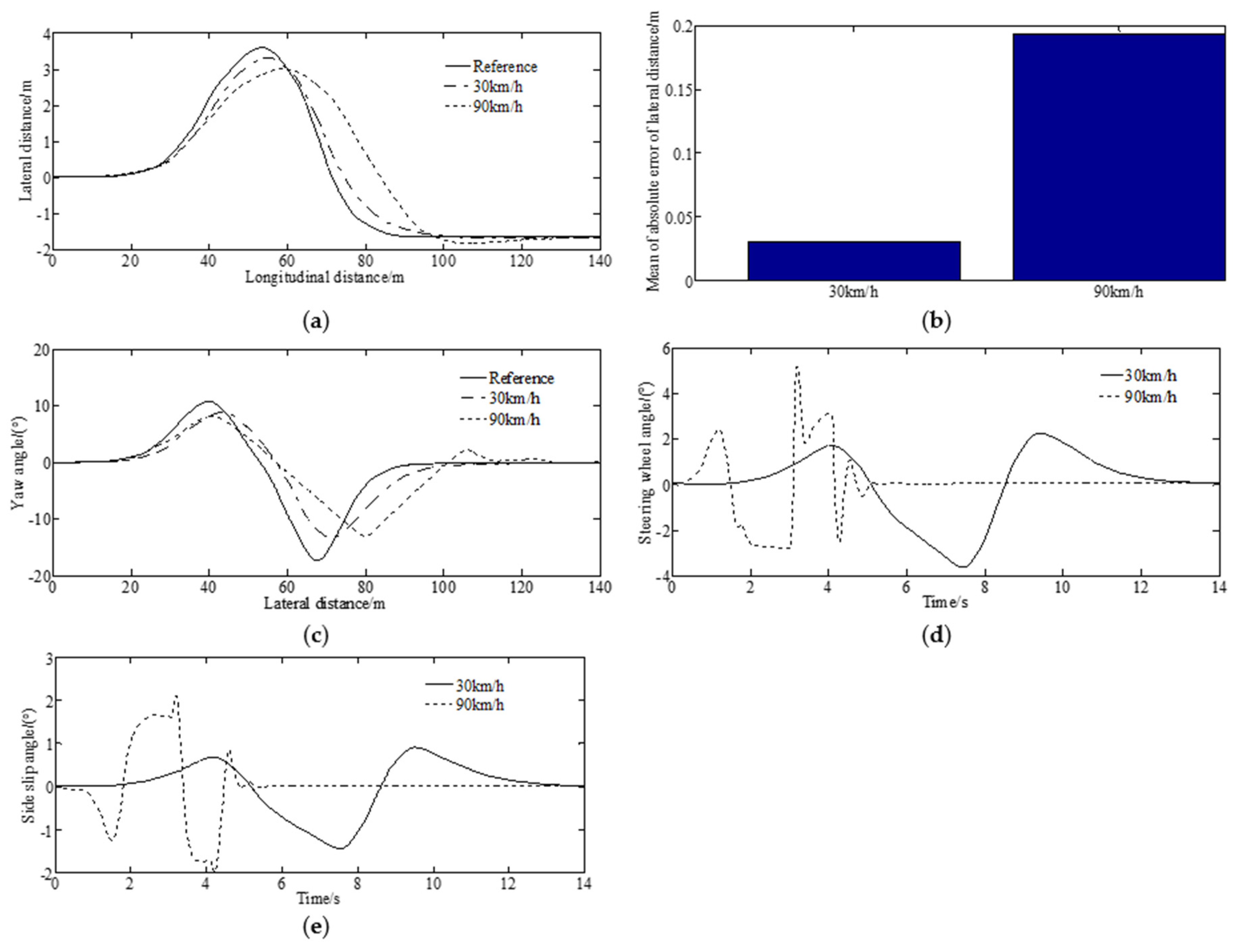
4.1. Numerical Simulations

This section uses CarSim to verify the feasibility and effectiveness of the optimal control problem for trajectory tracking. The CarSim simulation platform has the advantages of accuracy, convenience, good visualization, high cost-effectiveness, and real-time monitoring and has good practicality for this study.

For the simulations, the calculation parameters are shown in

Table 1. Simulation parameters.

Parameter	Definition	Value
m (kg)	vehicle mass	1265
Iz (kg∙m2)	moment of inertia around the z axis	1800
a (m)	distances of front axle from the center of gravity	1.170
b (m)	distances of rear axle from the center of gravity	1.195
k1 (N∙rad−1)	synthesized stiffness of front tire	60,042
k2 (N∙rad−1)	synthesized stiffness of rear tire	109,295
Iw (kg∙m2)	moment of inertia of the steering system	16.38
${\xi }_1/\mathrm{m}$	front wheel aligning arm of force	0.021
hg (m)	height of the center gravity	0.53

.

Figure 2 is the simulation result under the condition of different road friction coefficient.

From Figure 2a, it can be seen that when the vehicle is driving on a road with a lower road friction coefficient, the driving trajectory of the vehicle is more likely to deviate from the target trajectory, and there are larger fluctuations at turning points. When the vehicle travels on a road with a high road friction coefficient, its tracking trajectory can be maintained within a high accuracy range, and it tends to stabilize within a short displacement in the final straight section, without obvious oscillation. This is because that the ground with higher road friction coefficient can provide more lateral force for the tires and reduce lateral sliding. From Figure 2b, it can be seen that, the error of the lateral distance under the condition of $\mu =0.8$ is smaller than that of $\mu =0.4$. The main reason is that as the road attachment conditions get better, the ground can provide more lateral force to allow the tires, better to operate in the linear region and reduce lateral sliding. From Figure 2c, it can be seen that when the vehicle tracking the double lane changing road with lower road friction coefficient, the tracking error is bigger. However, under the control of the proposed method, the deviation finally converges to zero. From Figure 2d, it can be seen that although there is bigger error when the vehicle tracks the given wet road, the front steering angles satisfy the constraints, indicating the better control performance of the proposed method. Figure 2e indicates that when the vehicle exits the double lane changing road with a lower road friction coefficient, it generates a larger side slip angle, resulting in unstable operating conditions.

Figure 3 is the simulation result under the condition of different vehicle speeds.

As shown in Figure 3a, the vehicle completed the simulation on the double lane changing test road under the condition of u = 30 km/h smaller than that of u = 90 km/h, and the path tracking of the vehicle is relatively optimal at u = 30 km/h. From Figure 3b, it can be seen that, the error of the lateral distance under the condition of u = 30 km/h smaller than that of u = 90 km/h. The main reason for this is that as the speed increases, the coupling of the longitudinal movement introduces an error in the model. From Figure 3c, it can be seen that the path tracking and driving stability performance of the vehicle at u = 30 km/h are better than those at u = 90 km/h. When the vehicle is traveling at a higher speed, the trajectory of the vehicle is more likely to deviate from the target trajectory and experience significant fluctuations at corners. However, under the control of the proposed method, the deviation finally converges to zero. From Figure 3d, it can be seen that although there are bigger errors when the vehicle tracks the given path with the speed of u = 90 km/h, the front steering angles satisfy the constraints and remain in a small range, indicating the better control performance of the proposed method. Figure 3e indicates that when the vehicle exits the double lane changing road with u = 90 km/h, it generates a larger side slip angle, resulting in unstable operating conditions.

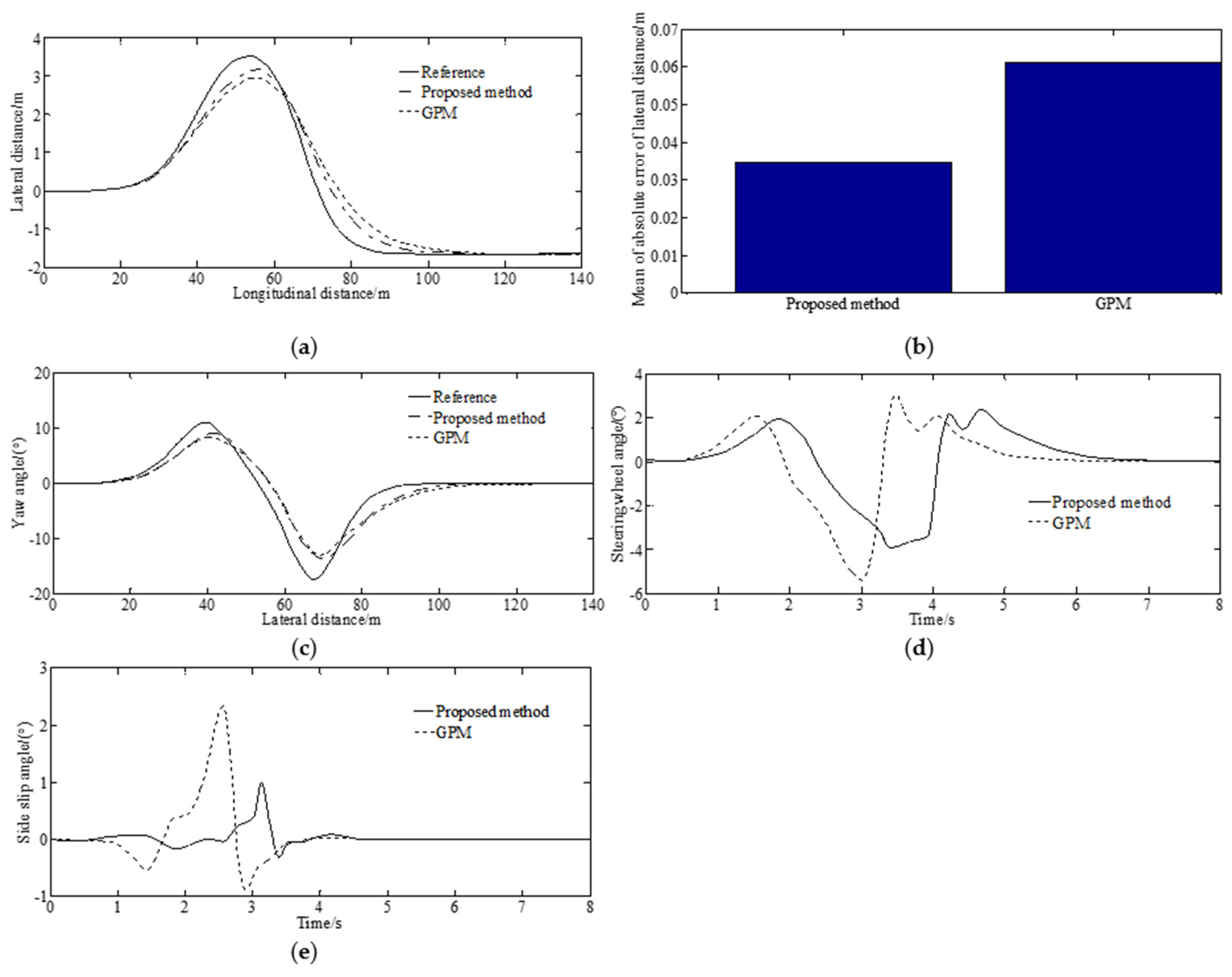
4.2. Control Performance

Figure 4 is the comparison of the control performance under the condition of different methods.

Figure 4a,b shows the comparison curve of lateral displacement and the tracking error. It can be seen that the improved hp adaptive pseudospectral method can track the reference path faster, with better path tracking accuracy and convergence speed as well as higher error of lateral distance than the GPM control method. As shown in Figure 4c, when the hp adaptive pseudospectral method is applied to the vehicle, the yaw angle can track the ideal one very well, and the convergence speed is fast. However, compared to the hp adaptive pseudospectral method, the GPM method has smaller fluctuations in the yaw angle during the control process with larger errors, and slower convergence speed. As shown in Figure 4d, during the steering process, the front wheel steering angle calculated using the GPM control algorithm is greater than that of the improved hp adaptive pseudospectral method. Figure 4e indicates that the amplitude of the sideslip angle of the improved hp adaptive pseudospectral method is less than the traditional GPM method.

Based on the above analysis results, it is not difficult to see that compared to the GPM method, the hp adaptive pseudospectral method has better path tracking accuracy, faster convergence speed, and ensures the lateral stability of the vehicle while improving path tracking accuracy.

Under the precision requirement of ε, three different pseudospectral methods are used to solve the same trajectory tracking problem, and the results are shown in

Table 2. Optimization comparison of different pseudospectral methods.

$\mathit{\epsilon }$	Method	${\mathit{K}}_{\mathbf{0}}$	${\mathit{N}}_{\mathbf{0}}$	$\mathit{E}$/10−5	$\mathit{t}$/s	Number of Iterations
10−3	p	1	20	93.25	3.9011	35
	h	5	4	52.98	2.5112	28
	Improved hp	5	4	52.79	3.2178	30
10−4	p	1	20	9.879	18.0531	165
	h	5	4	6.136	22.6529	96
	Improved hp	5	4	5.765	5.4912	70
10−5	h	5	4	0.936	14.2887	128
	Improved hp	5	4	0.643	7.0699	73

.

In the table, p is the global Radau pseudospectral method; h is the segmented fixed order Radau pseudospectral method, and hp is the hp adaptive Radau pseudospectral method. $K_0$, $N_0$, E, and t, respectively are the initial number of subintervals; the initial collocation number within the interval; the maximum error of the differential-algebraic constraint at the completion of optimization; and calculation time.

From Table 2, it can be seen that when the accuracy requirement is low, all three methods can optimize the results, and there is no significant difference in optimization speed and total number of collocation points. Under the same precision requirements, the improved hp pseudospectral method gradually demonstrated its advantages, both in terms of optimization speed and total number of collocation points, which are superior to the other two methods. As the accuracy requirements increase, the p method cannot obtain the optimal solution by simply increasing the number of collocation points, while the h and the improved hp methods successfully overcome the problem caused by roughness and obtain the optimal solution. Relatively speaking, the improved hp pseudospectral method outperforms the h method in terms of the total number of collocation points, subinterval partitioning, and optimization speed.

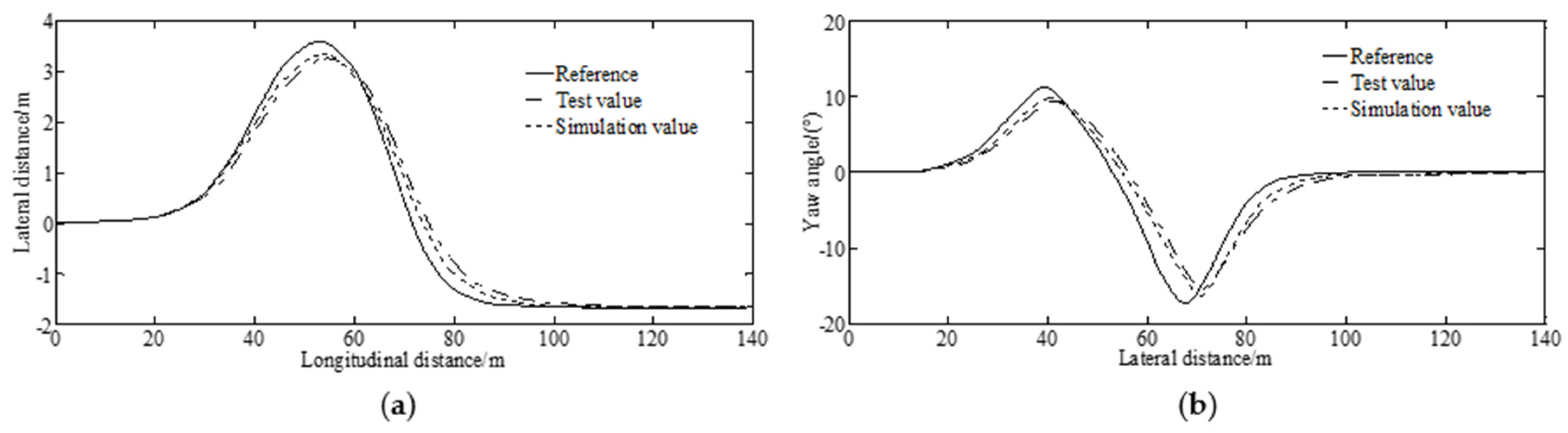
4.3. Experimental Verification

A virtual test adopting the Carsim software(2016) is conducted to verify the feasibility of the simulated results.

Carsim is a multifunctional software designed by Mechanical Simulation Corporation in the United States, mainly for simulating the dynamics of vehicles. It also has multiple vehicle models, road models, and driver models, and has a wide range of applications in traffic simulation and vehicle performance testing in multiple countries and regions.

The main features of Carsim software are as follows:

(1)

Accurate. The mathematical model of the Carsim is based on decades of research on vehicle dynamics characteristics. And with the continuous addition of new features, research is also ongoing. OEM users unanimously believe that the predicted results of CarSim are almost consistent with the actual test results.

(2)

Good scalability. The mathematical model of the Carsim covers the entire vehicle system, as well as input parameters from the driver, ground, and aerodynamics. These models can use built-in Vehicle Sim commands, MATLAB/SIMULINK(2018) from Mathworks, Lab VIEW from National Instruments (NI), as well as custom programs in Visual Basic, C language, and other languages to add higher-level control methods or extend existing subsystem and component models, such as tires, brakes, powertrains, etc.

Figure 5 shows the experimental results of lateral distance and yaw rate. The trends of the curve, the test value, and the simulation value as well as the reference are consistent, indicating that the trajectory tracking strategy based on the improved hp adaptive pseudospectral method can effectively control the vehicle to track the given trajectory while ensuring stability during complex trajectory driving and verifying the effectiveness of the proposed method. In summary, the proposed method can make the vehicle have good path tracking performance. Compared with traditional GPM, the path tracking control performance of the improved hp adaptive pseudospectral method is improved.

5. Conclusions

This article provides a general description and parameterization process of the optimal control problem based on trajectory tracking optimization. The continuity constraints are discretized using the hp adaptive pseudospectral method, and the optimal control problem is transformed into an NLP problem. The update criteria for adjusting the number of segments and increasing the number of collocation points using the hp adaptive pseudospectral method are analyzed in detail. Subsequently, the algorithm is used to analyze the performance indicators of path tracking with the shortest time under different road friction coefficients and vehicle speeds. The effectiveness and rationality of the proposed algorithm are verified via virtual experiments. The results show that the proposed method can make the vehicle track the given path well and has strong robustness to different road and vehicle speeds. Compared to the traditional methods, the proposed method in this article is better in terms of tracking performance of a given path. The path tracking and driving stability performance of the vehicle at lower speeds are better than those at higher speeds. And the tracking error of the lateral distance under the condition of $\mu =0.8$ is smaller than that of $\mu =0.4$. The optimal path tracking control using the improved hp adaptive pseudospectral method has higher accuracy and better control effect compared to traditional control algorithms. Although the control variables of the improved hp adaptive pseudospectral method are relatively more complex, the trajectory satisfies path constraints, indicating that the simulation results are feasible. In summary, the proposed method can make the vehicle have good path tracking performance. Compared with traditional GPM, the path tracking control performance of the improved hp adaptive pseudospectral method is improved.

The proposed control method is derived under the premise of small longitudinal velocity changes in the vehicle, and its robustness to time-varying vehicle speed and uncertain vehicle parameters needs further research. In addition, although the effectiveness of the proposed method has been validated in two typical scenarios, its applicability in real-world scenarios needs further verification. And also, the approach of Transport System Models (TSMs) should be considered for the path tracking research. Given the importance of accurate modeling in vehicle trajectory tracking. In the future, the effect of the exclusion of vertical and roll dynamics or tire relaxation behavior should be verified. And also, if the proposed control method’s effectiveness varies significantly under more complex or full vehicle dynamics models is also an important research direction.

References

1. Liu, Y.J.; Cui, D.W.; Peng, W. Optimum Control for Path Tracking Problem of Vehicle Handling Inverse Dynamics. Sensors 2023, 23, 6673. [Google Scholar] [CrossRef] [PubMed]
2. Liu, Y.J.; Cui, D.W. Estimation algorithm for vehicle state estimation using ant lion optimization algorithm. Adv. Mech. Eng. 2022, 14, 1–11. [Google Scholar] [CrossRef]
3. Liu, Y.J.; Cui, D.W.; Peng, W. Optimal Lane Changing Problem of Vehicle Handling Inverse Dynamics Based on Mesh Refinement Method. IEEE Access 2023, 11, 115617–115626. [Google Scholar] [CrossRef]
4. Zhao, S.E.; Hu, H.Y.; Jing, D.Y. Stability Control of Distributed Drive Electric Vehicle Based on AFS/DYC Coordinated Control. J. Huaqiao Univ. 2021, 42, 571–579. [Google Scholar]
5. Lu, M.X.; Xu, Z.C. Integrated handling and stability control with AFS and DYC for 4WID-EVs via dual sliding mode control. Autom. Control Comput. Sci. 2021, 55, 243–252. [Google Scholar]
6. Gao, X.; Ma, Y.; Toshiyuki, S.; Huang, H. Lateral coupling model of automatic platooning based on vehicle to vehicle communication. Automot. Eng. 2021, 43, 1745–1751. [Google Scholar]
7. Fassbender, D.; Heinrich, B.C.; Luettel, T.; Wuensche, H.-J. An optimization approach to trajectory generation for autonomous vehicle following. In Proceedings of the 2017 IEEE/RSJ International Conference on Intelligent Robots and Systems (IROS), Vancouver, BC, Canada, 24–28 September 2017; IEEE: Piscataway, NJ, USA, 2017; pp. 3675–3680. [Google Scholar]
8. Wei, S.; Zou, Y.; Zhang, X.; Zhang, T.; Li, X. An integrated longitudinal and lateral vehicle following control system with radar and vehicle-to-vehicle communication. IEEE Trans. Veh. Technol. 2019, 68, 1116–1127. [Google Scholar] [CrossRef]
9. Liu, Y.; Zong, C.; Zhang, D. Lateral control system for vehicle platoon considering vehicle dynamic characteristics. IET Intell. Transp. Syst. 2019, 13, 1356–1364. [Google Scholar] [CrossRef]
10. Chen, W.; Zhao, C.; Dai, G.; Zhao, Z. A partially flexible virtual trailer link model for vehicle-following systems. Trans. Inst. Meas. Control 2015, 37, 273–281. [Google Scholar] [CrossRef]
11. Bayuwindra, A.; Aakre, O.L.; Ploeg, J.; Nijmeijer, H. Combined lateral and longitudinal CACC for a unicycle-type platoon. In Proceedings of the 2016 IEEE Intelligent Vehicles Symposium (IV), Gotenburg, Sweden, 19–22 June 2016; IEEE: Piscataway, NJ, USA, 2016; pp. 527–532. [Google Scholar]
12. Duan, Y.; Zhang, Y.; Wang, Y.; Zeng, J.; Xu, P. A light-duty truck model for the analysis of on-center handling characteristics. Int. J. Veh. Perform. 2022, 8, 147–165. [Google Scholar] [CrossRef]
13. Park, M.; Lee, S.; Han, W. Development of steering control system for autonomous vehicle using geometry based path tracking algorithm. ETRI J. 2015, 37, 617–628. [Google Scholar] [CrossRef]
14. Kigezi, T.N.; Alexandru, S.; Mugabi, E.; Musasizi, P.I. Sliding mode control for tracking of nonholonomic wheeled mobile robots. In Proceedings of the IEEE 2015 5th Australian Control Conference (AUCC), Gold Coast, Australia, 5–6 November 2015; IEEE: New York, NY, USA, 2015; pp. 21–26. [Google Scholar]
15. Li, L.; Song, K.; Tang, G.; Xue, W.; Xie, H.; Ma, J. Active disturbance rejection path tracking control of vehicles with adaptive observer bandwidth based on Q-learning. Control Eng. Pract. 2025, 154, 106137. [Google Scholar] [CrossRef]
16. Wang, X.; Fu, M.; Ma, H.; Yang, Y. Lateral control of autonomous vehicles based on fuzzy logic. Control Eng. Pract. 2015, 34, 1–17. [Google Scholar] [CrossRef]
17. Ren, Y.; Zheng, L.; Zhang, W.; Yang, W.; Xiong, Z. A study on active collision avoidance control of autonomous vehicles based on model predictive control. Automot. Eng. 2019, 41, 48–54. [Google Scholar]
18. Chen, Y.; Zhang, H.; Zou, W.; Zhang, H.; Zhou, B.; Xu, D. Dynamic modeling and learning based path tracking control for ROV-based deep-sea mining vehicle. Expert Syst. Appl. 2025, 262, 125612. [Google Scholar] [CrossRef]
19. Li, D.; Leung, M.-F.; Tang, J.; Wang, Y.; Hu, J.; Wang, S. Generative Self-Supervised Learning for Cyberattack-Resilient EV Charging Demand Forecasting. IEEE Trans. Intell. Transp. Syst. 2025, 1–10. [Google Scholar] [CrossRef]
20. Cai, Y.; Li, J.; Sun, X.; Chen, L.; Jiang, H.; He, Y.; Chen, X. Research on hybrid control strategy for intelligent vehicle path tracking. China Mech. Eng. 2020, 31, 289–298. [Google Scholar]
21. Salzmann, F.; Gadi, S.; Gundlach, I. Racing line optimisation for an advanced driver assistance system. Int. J. Veh. Perform. 2021, 8, 46–73. [Google Scholar] [CrossRef]
22. Croce, A.I.; Musolino, G.; Rindone, C.; Vitetta, A. Traffic and Energy Consumption Modelling of Electric Vehicles: Parameter Updating from Floating and Probe Vehicle Data. Energies 2022, 15, 82. [Google Scholar] [CrossRef]
23. Liu, Y.J.; Cui, D.W.; Xie, C.L. Optimal control of lane changing problem of intelligent Vehicle. J. Vibroeng. 2025, 27, 120–133. [Google Scholar] [CrossRef]
Figure 1. 4-DOF vehicle model.
Wevj 16 00262 g001
Figure 2. Simulation result under the condition of different road friction coefficients: (a) lateral distance; (b) error of lateral distance; (c) yaw rate; (d) steering wheel angle; (e) side slip angle.
Wevj 16 00262 g002
Figure 3. Simulation result under the condition of different vehicle speeds: (a) lateral distance; (b) error of lateral distance; (c) yaw rate; (d) steering wheel angle; (e) side slip angle.
Wevj 16 00262 g003
Figure 4. Comparison results between the hp adaptive pseudospectral method and GPM: (a) lateral distance; (b) error of lateral distance; (c) yaw rate; (d) steering wheel angle; (e) side slip angle.
Wevj 16 00262 g004
Figure 5. Experimental results of lateral distance and yaw rate: (a) lateral distance; (b) yaw rate.
Wevj 16 00262 g005