User Cost Minimization and Load Balancing for Multiple Electric Vehicle Charging Stations Based on Deep Reinforcement Learning

Abstract

In the context of global energy conservation and emission reduction, electric vehicles (EVs) are essential for low-carbon transport. However, their rapid growth challenges power grids with load imbalances across networks and increases user charging costs. To address the issues of load balancing across large-scale distribution networks and the charging costs for users, this paper proposes an optimization strategy for EV charging behavior based on deep reinforcement learning (DRL). The strategy aims to minimize user charging costs while achieving load balancing across distribution networks. Specifically, the strategy divides the charging process into two stages: charging station selection and in-station charging scheduling. In the first stage, a Load Balancing Matching Strategy (LBMS) is employed to assist users in selecting a charging station. In the second stage, we use the DRL algorithm. In the DRL algorithm, we design a novel reward function that enables charging stations to meet user charging demands while minimizing user charging costs and reducing the load gap among distribution networks. Case study results demonstrate the effectiveness of the proposed strategy in a multi-distribution network environment. Moreover, even when faced with varying levels of EV user participation, the strategy continues to demonstrate strong performance.

1. Introduction

In the global effort to address climate change and reduce greenhouse gas emissions, electric vehicles (EVs) are playing an increasingly significant role, offering immense potential to enhance sustainability and environmental friendliness in urban areas [1]. With advancements in technology and proactive policy support, EVs are gradually becoming the mainstream market choice. According to statistics, the market share of EVs reached approximately 18% in 2023, compared to 14% in 2022 and only 2% in 2018 [2]. However, the widespread adoption of EVs has had a significant impact on the distribution of loads within power grids, thereby affecting the operation of distribution networks [3] and the charging costs for users. On the one hand, the charging behavior of EV users is highly uncertain; uncoordinated charging during peak periods may exacerbate the load on the distribution network, threatening the safe operation of the grid [4,5] and increasing user charging costs. On the other hand, as an important adjustable resource within the distribution network [6,7], EVs offer flexibility in terms of charging location and the controllability of the charging process. If EV charging behavior can be effectively guided and their flexibility fully utilized, it can not only mitigate the negative impact on the operation of distribution networks but also promote load balancing among distribution networks [8,9,10] and reduce user charging costs [11,12].

In recent years, significant progress has been made in academic research on EV charging behavior, which can be broadly divided into two categories. The first category focuses on optimizing the selection of charging stations for EVs to achieve effective coordination of charging behavior [11,12,13,14,15,16]. In this area of research, scholars guide users to specific charging stations based on different optimization objectives. For instance, in [11], a trip planning scheme for EVs aimed at minimizing user travel time and energy consumption was proposed, with consideration given to communication security between users and the dispatch center. In [12], a road speed matrix acquisition and recovery algorithm was developed based on crowd-sensing technology to optimize travel time and economic costs for EV users. Sortomme et al. [13] and Sun et al. [14] proposed EV dispatch strategies and graph game models, focusing on power grid losses and charging delays in the traffic network, respectively. Although these studies are abundant, most of them focus on minimizing grid losses or user charging costs, with less attention paid to the impact among distribution network loads. Chen et al. [15] introduced the issue of load balancing across multiple microgrids for the first time and proposed a charging station allocation strategy considering spatial load balancing. Based on [15], Xia et al. [16] further optimized the strategy by considering the load conditions of multiple microgrids during user service. However, these studies primarily focus on the selection of charging stations, while relatively neglecting the flexibility of EV users’ charging behavior within the stations.

Another category of research focuses on how to implement orderly charging control within charging stations for large-scale EVs. In recent years, this area of study has attracted widespread attention from scholars [17,18,19,20,21,22,23], with research methods covering heuristic algorithms [17], integer programming [18,19], the Alternating Direction Method of Multipliers (ADMM) [20], and model predictive control (MPC) methods [21,22,23,24]. For example, Liu et al. [17] used a genetic algorithm to solve the optimal charging scheduling problem under the constraint of a limited number of chargers. Sun et al. [18] achieved orderly charging within charging stations by solving two integer programming problems under the constraint of distribution network line capacity. Virgilio Pérez et al. [24] adjusted the charging power within charging stations based on grid information, electricity prices, and user preferences. By employing the MPC method, they effectively reduced user costs and mitigated load fluctuations in the distribution network. These methods typically optimize decision variables based on the global state of the environment and are model-based, requiring accurate modeling [17,18,19] or prediction of EV behavior [21,22,23,24]. However, in practice, accurately modeling the randomness of EV user arrivals or predicting their arrival outcomes is highly challenging. This makes these traditional model-based methods less effective for real-time scheduling of EVs.

In recent years, advancements in artificial intelligence (AI) technologies have significantly contributed to the optimization of EV charging management. Deep learning has been widely applied in predicting EV charging demand to optimize grid scheduling and resource allocation [25]. Furthermore, the efficient operation of smart grids relies on the coordinated optimization of communication, sensing, and computation. Studies have shown that the HTed SC method can significantly reduce communication, sampling, and computational loads in distribution networks, thereby improving system computational efficiency [26]. Meanwhile, the combination of deep learning and reinforcement learning has further enhanced reinforcement learning’s decision-making capability, enabling it to autonomously learn optimal strategies in complex environments. Deep Reinforcement Learning (DRL) is a model-free, online algorithm that can autonomously learn optimal strategies based on past and current environmental information, without requiring assumptions about the stochastic models of uncertain future events. Since DRL does not rely on explicitly modeling uncertainty, it can efficiently make decisions in dynamic environments. Based on this feature, numerous researchers have employed DRL to study orderly charging within charging stations [27,28,29,30]. Additionally, in the broader field of power grid optimization, multi-agent deep reinforcement learning (MADRL) has been utilized for adaptive reconfiguration of distribution networks, improving cost efficiency and security [31]. The successful application of this approach further demonstrates the potential of DRL in achieving efficient and real-time scheduling in complex power grid environments. For instance, Wan et al. [27] approached the problem from the user’s perspective, considering the uncertainties in travel and electricity prices, and used DRL to formulate the optimal charging strategy for users. In [28], the problem was considered from the perspective of charging stations, combining orderly charging with station pricing, and reinforcement learning was used to increase the overall revenue of the station. In [29], a fixed-dimensional matrix was used to anchor the state space of reinforcement learning, effectively addressing the dimensionality issue in DRL. Following [29], Chen et al. [30] further fixed the size of the action space, making it independent of the number of EVs. Despite the significant progress made in these studies, most research scenarios have been limited to a single charging station, failing to fully consider the interactions among the distribution networks where the charging stations are located.

From the existing literature, it can be observed that in the research on EV charging station selection, the load balancing algorithm proposed in [15] creatively utilizes EVs to address the issue of load imbalance across multiple microgrids, providing a solid foundation for research on spatial load balancing. However, it does not account for the charging flexibility of EV users once they arrive at the charging stations, which limits the overall system performance. In contrast, studies on the orderly charging of EVs successfully apply DRL to solve the orderly charging problem in a single EV charging station. Nevertheless, these studies fail to consider the impact of charging behavior on other distribution networks. To complement the previous work and fully exploit the flexibility of EV charging, while achieving both the minimization of charging costs and the load balancing across multiple distribution grids, this paper proposes a novel optimization strategy for the EV charging process. This strategy comprehensively considers the flexibility of EVs in both the selection of charging stations and the charging process within the stations, dividing the optimization of the charging process into two stages: charging station selection and in-station charging optimization.

The main contributions of this paper are listed as follows:

1.

Unlike previous studies that focused primarily on either charging station selection or on orderly charging for EVs within a single charging station, this paper considers both processes simultaneously. By fully leveraging the flexibility of EVs, this approach enhances their contribution to load balancing across distribution networks and reduces charging costs for EV users.

2.

This paper designs a novel DRL reward function that considers both EV users and power grids. This reward function can guide charging stations to implement an EV power distribution strategy that minimizes user charging costs while optimizing load balancing across distribution networks.

3.

The case study analyses demonstrate that this strategy remains effective even under varying levels of user participation.

The remainder of this paper is organized as follows: Section 2 introduces the charging station allocation model and the charging resource scheduling model, and formulates the orderly charging problem within charging stations as a Markov Decision Process (MDP) problem. Section 3 presents the EV charging station selection algorithm based on the Load Balancing Matching Strategy (LBMS) and the charging resource allocation algorithm based on the Double Deep Q Network (DDQN). Section 4 compares the system performance under different algorithms. We conclude this paper in Section 5.

2. System Model and MDP

2.1. Charging Station Allocation

In this paper, we consider a city with M distribution networks, which are uniformly distributed across different regions. Each distribution network adopts a hybrid model integrating distributed energy resources (DERs) and energy storage systems (ESSs), offering greater independence and stability compared to traditional power grids [32]. These distribution networks can flexibly integrate renewable energy sources and optimize energy management through intelligent scheduling systems, thereby improving energy utilization efficiency. Moreover, the energy storage system can be combined with vehicle-to-grid (V2G) technology, enabling EVs not only to act as power loads for charging but also to feed energy back into the grid when needed. This integration further enhances the flexibility and balancing capability of the power system. Additionally, by incorporating AI technologies, these distribution networks can dynamically adjust energy distribution and charging scheduling using reinforcement learning, intelligent optimization, and data-driven prediction, further improving the system’s adaptability and overall operational efficiency. Each distribution network is equipped with a large aggregator that connects all charging facilities within the area, thereby unifying the management of all charging facilities in the distribution network into a single huge charging station. The model employed in this paper is a time-series model, in which time is divided into several equidistant time windows of fixed duration $\Delta T$, and at the beginning of each time window, a number of EV users make charging requests.

Due to the variation in the areas served by different distribution networks (such as industrial and residential zones), there are significant differences in peak electricity demands across these regions. As a result, the base load of the distribution networks fluctuates considerably over time, with notable load disparities among different networks. Figure 1 illustrates these load variations, reflecting the differences in the load levels across distribution networks at different times. Moreover, the distribution of EVs adjusts dynamically based on the current load conditions of the distribution networks, with vehicle locations changing in response to load variations. At every moment, the load among the distribution networks has a minimum and maximum value, denoted as $P_{valley}\left(t\right)$ and $P_{peak}\left(t\right)$, respectively. Specifically, $P_{valley}\left(t\right)$ represents the valley power load of distribution networks at time t, and $P_{peak}\left(t\right)$ represents the peak power load of distribution networks at time t.

When the battery levels of EV users are low, they will search for a charging station to park and charge until their charging needs are met or the predetermined parking time is reached. The distance between the EV user and the charging station plays a crucial role in the selection process. Without proper guidance, users tend to choose the nearest charging station, and this uncoordinated charging behavior may result in users gravitating toward distribution networks with higher loads, potentially affecting load balancing among grids.

To ensure the load balancing of the power grids, it is essential to provide reasonable guidance in the selection of charging stations for EV users. In this context, the vehicle scheduling center should guide EV users to recommended charging stations, thereby optimizing charging behavior. The core objective of the scheduling center is to ensure the safe operation of the power grids. Therefore, when recommending charging stations, the scheduling center must consider not only the geographical locations of stations to ensure that users can reach stations with their remaining battery capacity, but also the current electrical loads of various distribution networks to balance the system’s demand and supply. This guidance and scheduling strategy within the system is critical for the management of EV charging and contributes to maintaining the stability and safety of the power grids.

Specifically, when EV i requests for charging at time t, the scheduling center receives information regarding the EV’s current position $(x_i,y_i)$, as well as its initial state of charge (SOC) $S_i^{ini}$. The scheduling center calculates the distances from the location of EV i to various charging stations. In this paper, a matrix $\mathit{R}$ is utilized to store the distances from EV users to each charging station, and matrix $\mathit{R}$ is defined as

$$\begin{array}{c}\hfill \mathit{R}=\left[\begin{array}{cccc}{R}_{1,1}& R_{1,2}& \cdots & R_{1,M}\\ R_{2,1}& R_{2,2}& \cdots & R_{2,M}\\ ⋮& ⋮& \ddots & ⋮\\ R_{N,1}& R_{N,2}& \cdots & R_{N,M}\end{array}\right]\end{array}$$

(1)

where $R_{i,j}$ represents the distance from EV i to charging station j, and N denotes the number of EVs requesting charging.

Subsequently, the scheduling center calculates the distance that EV i can travel based on its initial SOC $S_i^{ini}$, denoted as $R_i$. This distance $R_i$ must satisfy inequality constraint

$$\begin{array}{c}\hfill R_i\le R^{max}{S}_i^{ini}\end{array}$$

(2)

where $R^{max}$ represents the maximum driving range of the EV when fully charged. By calculating $R^{max}{S}_i^{ini}$, the maximum distance that EV i can travel under its initial battery charge state can be determined. Combining the matrix $\mathit{R}$ with this formula, the scheduling center identifies a set of candidate charging stations for EV i, denoted as ${\mathit{C}\mathbf{\text{and}}}_i$. This candidate set ${\mathit{C}\mathbf{\text{and}}}_i$ is selected using the formula

$$\begin{array}{c}\hfill {\mathit{C}\mathbf{\text{and}}}_i=\left\{V_j^G|R_{i,j}\le R^{max}{S}_i^{ini}\right\}\end{array}$$

(3)

where $V_j^G$ represents charging station j that satisfies the above formula. The scheduling center will recommend an appropriate charging station j for the EV from this candidate set.

In this paper, the primary objective of recommending charging stations for EVs is to reduce load disparities among distribution networks. To evaluate the load distribution across the distribution networks at time t, we introduce the Spatial Load Valley-to-Peak Ratio (SLVTPR), denoted as $\eta \left(t\right)$. Its calculation is based on the total load of the entire distribution network, which includes both the base load (e.g., residential or industrial demand) and the additional load induced by EV charging within charging stations. $\eta \left(t\right)$ is defined by the equation

$$\begin{array}{c}\hfill \eta \left(t\right)={\displaystyle \frac{P_{valley}\left(t\right)}{P_{peak}\left(t\right)}}\times 100\%.\end{array}$$

(4)

The SLVTPR reflects the degree of disparity among peak and valley loads across distribution networks. A higher SLVTPR indicates more balanced loads among the distribution networks, signifying smaller extreme differences and more stable grid operation. Therefore, to achieve load balancing among distribution networks, the LBMS strategy is used in the allocation of charging stations. Specifically, the scheduling center needs to allocate EVs to the charging station with the minimal power load within their reachable range at time t, which can be expressed as

$$\begin{array}{c}\hfill j=arg\underset{j}{min}{P}_{j,t},j\in {\mathit{C}\mathbf{\text{and}}}_i\end{array}$$

(5)

where $P_{j,t}$ represents the sum of the loads of the distribution network where charging station j is located at time t.

After determining the charging station, the scheduling center will calculate the time at which the user arrives at charging station j. In this paper, it is assumed that the EV travels at a constant speed on the road, denoted as v. Therefore, the travel time $T_{i,j}^{tra}$ for EV i can be calculated using the equation

$$\begin{array}{c}\hfill T_{i,j}^{tra}={\displaystyle \frac{R_{i,j}}{v}}.\end{array}$$

(6)

Based on the travel time $T_{i,j}^{tra}$ and the time $t_i^0$ when EV i initiates the charging request, the charging start time $T_i^{str}$ can be determined as

$$\begin{array}{c}\hfill T_i^{str}=t_i^0+T_{i,j}^{tra}.\end{array}$$

(7)

Using the aforementioned methods, the scheduling center assigns EVs to appropriate charging stations.

2.2. Charging Resource Scheduling

When EV i arrives at charging station j, the operator needs to arrange charging resources for the EV. In this section, we analyze the charging arrangements for EVs at charging station j.

In this paper, to facilitate more convenient control of EV charging behavior, the charging service provided by the station follows an on–off strategy. This strategy implies that EVs connected to the charging piles will only operate in either full-power charging or zero-power charging modes.

Assuming that the number of charging piles at the charging station is sufficient, EVs can immediately connect to a charging pile and begin charging upon arrival at the station. Let $I_t$ represent the set of EVs arriving at the station at time t, $J_t$ the set of EVs that arrived before time t and have not yet completed their charging requirements, and $K_t=I_t\cup J_t$ the set of EVs requiring charging at time t. For any EV i, once it connects to a charging pile, the charging station can immediately access the user’s charging demand $d_i$, the estimated parking time $p_i$, and the start time of charging $T_i^{str}$.

In practical operations, the charging station operator makes decisions about charging EVs within the station only at the beginning of each $\Delta T$. Therefore, in this section, time is discretized into $T^{tot}$ time slots, with each time window having a length of $\Delta T$.

The smart charging agent (hereafter referred to as the agent) accesses user information at the start of each $\Delta T$, and since the agent makes decisions at discrete time points, it needs to calculate the charging time slots required by the user in the continuous charging condition (hereafter referred to as the required charging time slots) $c_{i,t}$ at time t and the estimated parking time slots $e_{i,t}$ at time t. In order to ensure that the user can complete the charging demand within the available parking time slots, this paper rounds up the required charging time slots and rounds down the estimated parking time slots during discretization. Assuming that the time interval between the two decision times is $\Delta T$, the required charging time slots $c_{i,t}$ and the estimated parking time slots $e_{i,t}$ are given as

$$\begin{array}{cc}\hfill c_{i,t}& =⌈{\displaystyle \frac{d_i}{\Delta Tp}}⌉,\forall i\in I_t\hfill \end{array}$$

(8)

$$\begin{array}{cc}\hfill e_{i,t}& =⌊{\displaystyle \frac{p_i}{\Delta T}}⌋,\forall i\in I_t\hfill \end{array}$$

(9)

where p represents the charging power of the charging station.

It can be observed that over time, both $c_{i,t}$ and $e_{i,t}$ will gradually decrease until $c_{i,t}$ or $e_{i,t}$ decreases to 0.

Therefore, the information of the EV is transformed into a three-dimensional vector ($c_{i,t}$, $e_{i,t}$, $T_i^{str}$). The agent needs to find the appropriate $c_{i,t}$ time slots for user charging before the parking time slots $e_{i,t}$ expires. The charging urgency $\Delta T_{i,t}^{emr}$ at time t for each user can be calculated as

$$\begin{array}{c}\hfill \Delta T_{i,t}^{emr}={\displaystyle \frac{c_{i,t}}{e_{i,t}}},\forall i\in K_t.\end{array}$$

(10)

From the above equation, it can be seen that $\Delta T_{i,t}^{emr}$ is a value between 0 and 1. At every moment, the agent calculates the urgency of charging for each EV. As $\Delta T_{i,t}^{emr}$ increases, the user’s charging demand becomes more urgent. The agent can adjust the charging order based on the urgency of the users, ensuring that the charging station meets the users’ charging demands while achieving the desired optimization objectives.

2.3. Markov Decision Process

By analyzing the aforementioned scenario within the charging station, it can be concluded that at the beginning of each time slot, the agent determines the charging schedule for the current time slot based on observations of the past and current charging time slots and estimated parking time slots of EVs. This decision, in turn, affects the remaining charging demand in future time periods. Therefore, the environment of orderly charging for EVs within a charging station exhibits Markov properties, and the solution to the optimal decision-making process is referred to as the solution to the MDP. Typically, the MDP model is represented by a four-tuple {S, A, P, R}, where the elements of the tuple denote the state of the environment, the actions taken by the agent, the transition probabilities of the environment, and the rewards obtained by the agent, respectively. Through continuous interaction with the environment, the agent gradually learns the optimal policy.

2.3.1. State

To address the curse of dimensionality in DRL, this paper employs a two-dimensional matrix to discretize EV feature information, as illustrated in Figure 2. In Section 2.2, an EV’s feature can be represented as ($c_{i,t}$, $e_{i,t}$, $T_i^{str}$). By ignoring $T_i^{str}$, the user feature information within a charging station can be simplified to ($c_{i,t}$, $e_{i,t}$). The agent only needs to access the user feature information within the charging station, count the number of users with the same (c, e), and store these data in the corresponding position of the matrix to complete the discretization process. Finally, by concatenating the matrix elements with the current time t, the state $s_t$ can be formally expressed as follows:

$$s_t=\left[N_t^{1,1},N_t^{1,2},\cdots ,N_t^{1,E^{max}},N_t^{2,1},N_t^{2,2},\cdots ,N_t^{c,e},\cdots ,N_t^{C^{max},E^{max}},t\right]$$

(11)

where $N_t^{c,e}$ represents the total number of EVs with remaining charging time slots c and expected parking time slots e at time t. $C^{max}$ denotes the maximum charging time for EVs, and $E^{max}$ represents the maximum parking time for EVs.

Moreover, since $c\le e$ (because once c exceeds e, even if the EV continues charging during the remaining parking period, it will still be unable to meet the charging demand), and both the charging demand and parking time for EVs are bounded, the dimensionality of the state space $S_{dim}$ can be computed as

$$\begin{array}{c}\hfill S_{dim}=C^{max}{E}^{max}-{\displaystyle \frac{C^{max}\left(C^{max}-1\right)}{2}}+1\end{array}$$

(12)

It can be seen that through this method, the state dimensionality can be fixed. This state representation preserves necessary information while reducing the complexity of the state space, thereby providing a more efficient computational framework for the agent’s decision-making process.

The aforementioned analysis of the state is specific to a particular charging station. In this paper, considering there are M large charging stations, the same analytical method can be applied to determine the state of charging station j at time t.

2.3.2. Action

In this paper, the action $a_{j,t}$ is defined as the ratio of the number of charging EVs $N_{j,t}^c$ to the total number of EVs $N_{j,t}^{tot}$ at station j at time t. Therefore, the action selected by the agent must satisfy the constraint

$$\begin{array}{c}\hfill 0\le a_{j,t}={\displaystyle \frac{N_{j,t}^c}{N_{j,t}^{tot}}}\le 1\end{array}$$

(13)

It can be seen that the action $a_{j,t}$ only indicates the number of charging EVs but does not specify which EVs should be served at time t. Therefore, it is necessary to determine a charging order to select which users will be provided with service. In this paper, an optimal Least Laxity First (LLF) charging strategy based on the urgency of user demand is used to determine which EVs should be prioritized for charging operations.

In (10), $\Delta T_{i,t}^{emr}$ was defined to represent the urgency of users’ charging demands. For users with larger $\Delta T_{i,t}^{emr}$, the gap between the required charging time and the estimated parking time is smaller, indicating a higher urgency. These users must maintain a fully charged state as much as possible before leaving the charging station; otherwise, there is a risk of not meeting their charging needs. Therefore, these users should be prioritized for charging. For users with the same $\Delta T_{i,t}^{emr}$, their charging urgency is identical, so users with smaller $e_{i,t}$ (remaining parking time) should be prioritized. This is because, for users with the same $\Delta T_{i,t}^{emr}$, the risk of not fulfilling their charging demand is the same. However, for users with shorter remaining parking times, the available charging time slots are fewer, and the risk of not meeting their charging needs is higher, so it is crucial to prioritize meeting the needs of these users.

Therefore, by combining the action with the LLF charging strategy, the agent can determine which users should be provided with charging services at time t.

2.3.3. State Transition

Given $s_t$ and $a_t$, and the system state will be transited to $s_{t+1}$ with the probability $\mathit{P}$ as follows:

$$\begin{array}{c}\hfill \mathit{P}(s_t,s_{t+1})=\mathbf{Pr}(s_{t+1}\mid s_t,a_t)\end{array}$$

(14)

Based on $s_t$ and $a_t$, EVs previously stationed at the charging station can transition into one of three states: (1) delayed charging, (2) charging, or (3) charging completion. Meanwhile, at this decision-making moment, additional EVs may arrive at the charging station and wait for charging. The state transition probabilities are influenced not only by the actions of EVs already at the station but also by the charging demands and parking durations of newly arriving EVs. Since these factors are dynamically changing and inherently unpredictable, the state transition probabilities cannot be explicitly formulated. Therefore, in the subsequent sections, a DRL-based approach will be introduced to learn and approximate these transition probabilities through interaction with the environment.

2.3.4. Reward

The optimization objectives of this paper are twofold. The first optimization objective is to minimize the charging cost for users. Therefore, the optimization objective for charging station j can be expressed as

$$\begin{array}{c}\hfill r_{j,t}^{cost}=a_{j,t}{N}_{j,t}^{tot}{p}_{j,t}\end{array}$$

(15)

where $p_{j,t}$ represents the price of charging station j at time t.

The second optimization objective is to minimize the load disparity among multiple distribution networks, which can be expressed as

$$\begin{array}{c}\hfill r_{j,t}^{disp}=a_{j,t}{N}_{j,t}^{tot}\left({\displaystyle \frac{P_{j,t}^{ini}}{P_t^{tot}}}-{\displaystyle \frac{1}{M}}\right)=a_{j,t}{N}_{j,t}^{tot}{l}_{j,t}\end{array}$$

(16)

where $P_{j,t}^{ini}$ represents the baseline load of the distribution network j at time t when no EV users are charging, $P_t^{tot}$ represents the total baseline load of all distribution networks at time t when no EV users are charging, and $l_{j,t}$ represents the difference between the proportion of the baseline load of distribution network j at time t in the total baseline load and the proportion of the ideal load for the distribution network.

Due to the significant differences in the quantitative scales of charging station prices and the load disparity among grids, it is necessary to normalize both factors in order to jointly optimize user charging costs and the load disparity among distribution networks. The normalization formula is given as

$$\begin{array}{c}\hfill x^{nor}={\displaystyle \frac{x^{max}-x_t}{x^{max}-x^{min}}}\end{array}$$

(17)

where $x^{nor}$ represents the normalized value, $x_t$ represents the value of the element at time t, $x^{max}$ represents the maximum value of the same type of element, and $x^{min}$ represents the minimum value of the same type of element.

According to (17), by normalizing both the charging price and the spatial load disparity among distribution networks to the same level, the charging price $p_{j,t}$ in (15) is normalized to $p_{j,t}^{nor}$, and the difference between the load proportion of the distribution network and the ideal load proportion $l_{j,t}$ in (16) is normalized to $l_{j,t}^{nor}$. Thus, the total immediate reward $r_{j,t}$ of charging station j can be expressed as

$$\begin{array}{c}\hfill r_{j,t}=\alpha a_{j,t}{N}_{j,t}^{tot}{p}_{j,t}^{nor}+\beta a_{j,t}{N}_{j,t}^{tot}{l}_{j,t}^{nor}\end{array}$$

(18)

where $\alpha$ and $\beta$ represent the weight factors in the reward function for minimizing user charging costs and balancing the load among distribution networks, respectively, ranging from 0 to 1.

The goal of agent is to maximize the total reward value for all decision points, and each decision point’s reward value includes both the immediate reward at the current moment and the future reward. Therefore, at each time step, the state-action function $Q_j^{\pi }(s,a)$ can be computed as

$$\begin{array}{c}\hfill Q_j^{\pi }(s,a)=\mathbb{E}\left[{\displaystyle \sum _{k=0}^{\infty }}{\gamma }^k{r}_{j,t+k}\mid s_t=s,a_t=a\right]\end{array}$$

(19)

where $\mathbb{E}$ represents the expectation function, $\gamma$ denotes the discount factor, and $r_{t+k}$ represents the reward the agent will receive at future time steps. $Q_j^{\pi }(s,a)$ represents the cumulative reward the agent can obtain by taking action a in state s, and then following an optimal policy thereafter. The discount factor $\gamma$ is used to reduce the weight of future rewards relative to immediate rewards, indicating how much the agent values future rewards. A higher $\gamma$ focuses on long-term gains, while a lower $\gamma$ emphasizes short-term rewards. To prevent the agent from only considering immediate rewards, $\gamma$ is typically set to a value close to 1. The value function $Q_j^{\pi }(s,a)$ measures the quality of taking action a in state s, influencing the agent’s selection of actions. The DRL algorithm is ultimately about selecting the best action from all available actions to maximize the total reward value.

3. The DDQN DRL Algorithm for Charging Station

The Deep Q Network (DQN) is a technique that combines deep learning with reinforcement learning. It builds upon the traditional Q-learning algorithm by incorporating deep neural networks to approximate the Q-function in Q-learning, enabling DQN to handle high-dimensional state space problems. Additionally, DQN introduces techniques such as experience replay and fixed Q-targets, which have enabled DQN to achieve significant advancements in the field of DRL. However, similar to traditional Q-learning, DQN updates the Q-values by selecting the maximum Q-value of the next predicted state. Specifically, the formula for updating the target Q-values in DQN is

$$\begin{array}{c}\hfill q_{target}=r_t+\gamma \underset{a^{\prime }}{max}Q(s^{\prime },a^{\prime })\end{array}$$

(20)

where $s^{\prime }$ represents the next state, and $a^{\prime }$ represents all possible actions in state $s^{\prime }$. It can be observed that this method of updating the Q-value assumes that the maximum Q-value corresponds to the best future return. However, in practical applications, due to various objective factors such as estimation errors, sampling errors, or noise, this maximization operation often leads to an overestimation of the Q-value. Given the inherent approximation errors of neural networks and the uncertainty of the environment, this bias can be further amplified. The issue of overestimation can cause the learned policy in the DQN algorithm to deviate from the optimal policy, significantly reducing the algorithm’s performance. Furthermore, overestimation can also affect the convergence of the algorithm, causing it to converge on a suboptimal policy, thereby negatively impacting overall effectiveness.

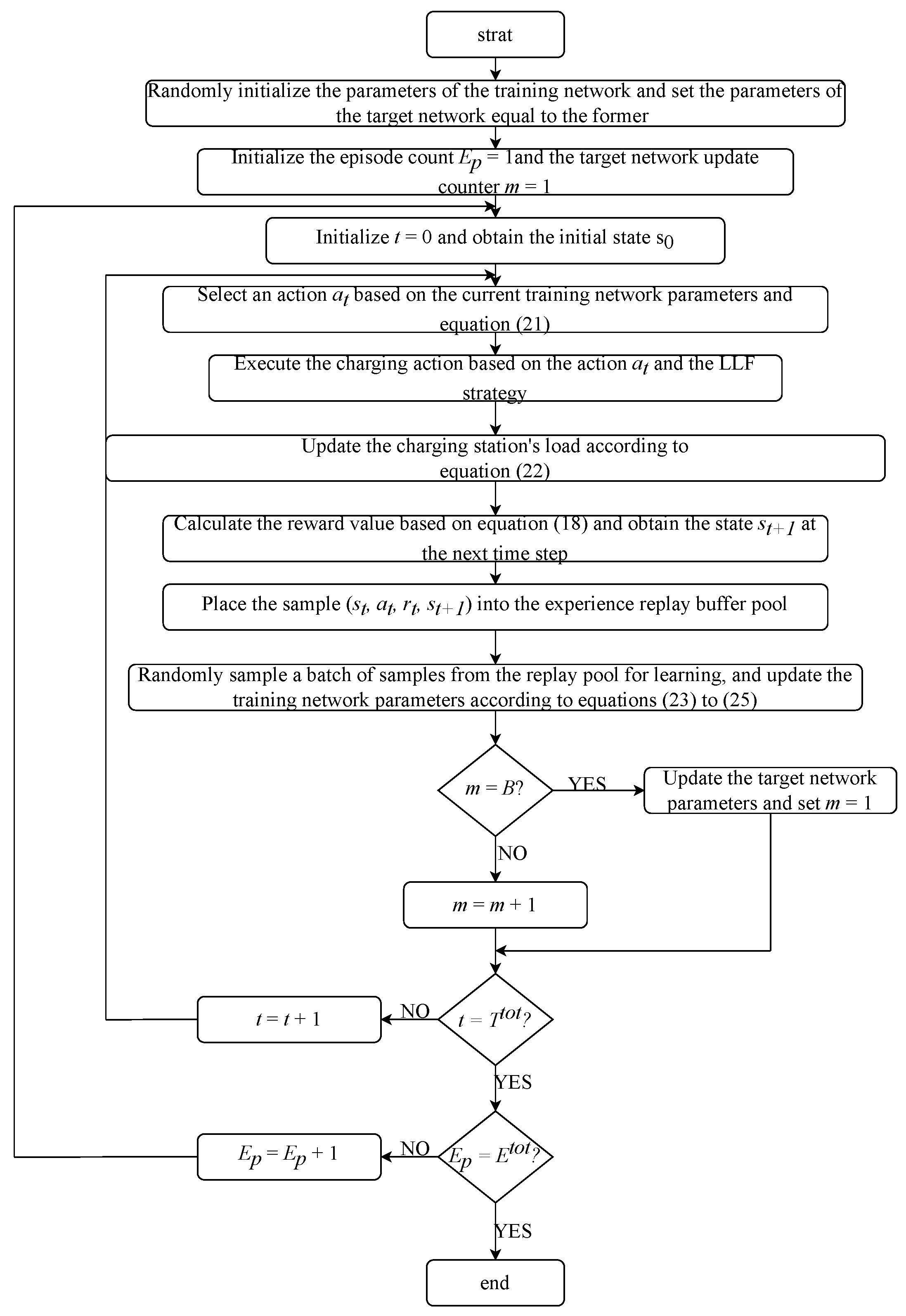
To address the overestimation problem in DQN, DDQN was proposed. DDQN mitigates overestimation by decoupling the max operation in the target Q-value calculation into two parts: action selection based on the training network and value estimation based on the target network. This effectively reduces overestimation, leading to more accurate and reliable target Q-value estimates, thereby improving the overall quality of the policy and the stability of the algorithm. The process of the DDQN algorithm within the charging station is presented in the following section and the specific training algorithm of DDQN is shown in Figure 3.

First, two neural networks with the same structure but independent parameters are initialized, one as the training network $Q\left(\theta \right)$ and the other as the target network $Q\left(\overline{\theta }\right)$. The parameters of the training network are initialized as $\theta$, and the same parameters are used in the target network, i.e., $\theta =\overline{\theta }$. Then, the total number of training episodes $E^{tot}$ and the target network parameter update frequency B are set.

Next, the initial state $s_0$ of the EV charging station is generated, and the training network selects an action using the $ϵ$-greedy strategy, i.e.,

$$\begin{array}{c}\hfill a_t=\left\{\begin{array}{cc}argmaxQ(s,a\mid \theta ),\hfill & \lambda \ge ϵ\hfill \\ random{a}_t\in A,\hfill & \lambda <ϵ\hfill \end{array}\right.\end{array}$$

(21)

where $ϵ$ represents the exploration rate, a value that gradually decreases from 1 to 0; $\lambda$ is a random number between 0 and 1; and A is the set of actions available for the agent to choose from.

After selecting action $a_t$, the load $P_{j,t}$ of charging station j is updated as

$$\begin{array}{c}\hfill P_{j,t}=P_{j,t}^{ini}+a_{t}p\end{array}$$

(22)

Finally, the agent chooses which users to charge at time t based on the urgency of user demand using the LLF charging strategy. The agent then calculates the immediate reward $r_t$ for the selected action. Next, the agent obtains the next state $s_{t+1}$ at the following time step. The tuple $(s_t,a_t,r_t,s_{t+1})$ is stored in the experience replay buffer. Finally, the agent randomly samples a batch $(s_t,a_t,r_t,s_{t+1})$ from the experience replay buffer and updates the parameters of the training network according to the equations

$$\begin{array}{c}\hfill q_{target}=r_t+\gamma \underset{a^{\prime }}{max}Q(s^{\prime },arg\underset{a^{\prime }}{max}Q(s^{\prime },a^{\prime };\theta );\overline{\theta })\end{array}$$

(23)

$$\begin{array}{c}\hfill L\left(\theta \right)=\mathbb{E}\left[{(q_{target}-Q(s,a\mid \theta ))}^2\right]\end{array}$$

(24)

$$\begin{array}{c}\hfill \theta =\theta -\mu {\mathrm{\nabla }}_{\theta }L\left(\theta \right)\end{array}$$

(25)

where $\mu$ is the learning rate, and ∇ represents the gradient operator.

By comparing (20) and (23), we can observe the key differences between the DDQN algorithm and the DQN algorithm. In DDQN, the update of the target Q-value relies on the cooperation of two networks: the training network is used for action selection, while the evaluation of the selected action’s value is performed by the target network. This decoupling strategy effectively mitigates the overestimation issue commonly encountered in DQN algorithms. The agent evaluates the difference between the predicted Q-value and the target Q-value using (24) and computes the gradient of the loss function with respect to the network parameters using (25), which is then used to update the parameters of the training network. Once the time reaches $T^{tot}$, the current training episode ends, and the next episode begins. This process is repeated until the predefined number of training episodes $E^{tot}$ is completed. During each episode, after every B training steps, the parameters of the training network are copied to the target network.

4. Simulation and Analysis

4.1. Parameter Setting

In this study, the basic load of the power distribution network and the hourly electricity price are based on real-world data. The base load data for the distribution network are derived from actual demand data in California and Nevada, USA [33]. After scaling according to a certain ratio, the data are randomly assigned to the distribution network. Then, according to the basic load of the distribution network, the time-of-use electricity price is formulated [17]. This paper adopts the DC charging method, and the distribution networks are evenly distributed in the city. The number of EV users requesting charging is based on the setting in [15]. At the beginning of each time slot, a certain number of users request charging. However, the distribution of these requests is positively correlated with the load levels of the respective distribution network areas. Specifically, areas with higher loads tend to have a greater number of users requesting charging. The DDQN training process was conducted on a PC with an i9-10900k CPU at 3.70 GHz. The program was implemented in Python 3.7 and simulated using TensorFlow 1.13. The MDP formulation in this paper is similar to that in [30], and therefore, some DDQN parameters were set with reference to its configuration. However, given the larger scale and higher complexity of our problem, certain hyperparameters we re adjusted and validated through multiple simulations. The final parameter settings are presented in

Table 1. Parameter settings.

Parameter	Value
Maximum charging time slots for EVs	7
Maximum parking time slots for EVs	12
Time window	00:00–23:55
Scope of city	30 × 30 km
State dimension	64
Action space	[0,0.1,0.2,...,1]
Number of hidden layers in network	2
Number of neurons per hidden layer	128
Activation function	ReLU
$\gamma$	0.95
$\mu$	0.0005
Batch size	64
B	5
$E^{tot}$	80,000
$\Delta T$	15
$T^{tot}$	96
M	4
p	20 kW
v	30 km/h
$R^{max}$	300 km

.

In each simulation, we compare four different charging strategies, which are detailed as follows:

• greedy: This charging strategy only considers LBMS. In this strategy, EVs begin charging immediately upon arrival.
• DRL_Space: The optimization objective of the DDQN algorithm is to minimize the load imbalance among distribution networks.
• DRL_Cost: The optimization objective of the DDQN algorithm is to minimize the users’ charging costs.
• DRL_Both: The optimization objective of the DDQN algorithm is to simultaneously minimize the users’ charging costs and the load imbalance among distribution networks.

4.2. Convergence of the DRL Algorithm

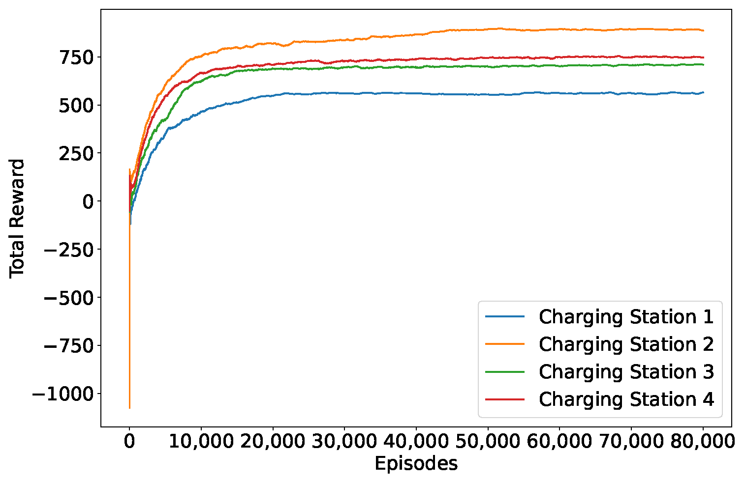
Using the parameter settings from Table 1, we configure the neural network and conduct a comparative analysis of the convergence performance of the DDQN algorithm under different optimization objectives. Figure 4, Figure 5 and Figure 6 illustrate the convergence behavior of the algorithm under the DRL_Space, DRL_Cost, and DRL_Both strategies when the number of EVs requesting charging is set to 1250.

These figures reveal distinct learning patterns under different strategies. At the early stages of training, the high exploration rate leads the agent to attempt a variety of actions, resulting in significant fluctuations in the total reward, which gradually increases as training progresses. As training continues, the exploration rate gradually decreases, shifting the agent’s behavior from exploration to exploitation, causing the reward values to stabilize and eventually converge. The final convergence of the reward values demonstrates that the proposed MDP formulation exhibits stable performance under the DDQN algorithm.

However, as observed from the three figures, the final converged reward values vary across different strategies. Additionally, convergence alone does not indicate that the agent has learned the optimal policy. Therefore, in the following sections, we will further validate and evaluate the learned policies to assess their effectiveness in achieving the desired optimization goals.

4.3. Performance of EV Charging Station Allocation

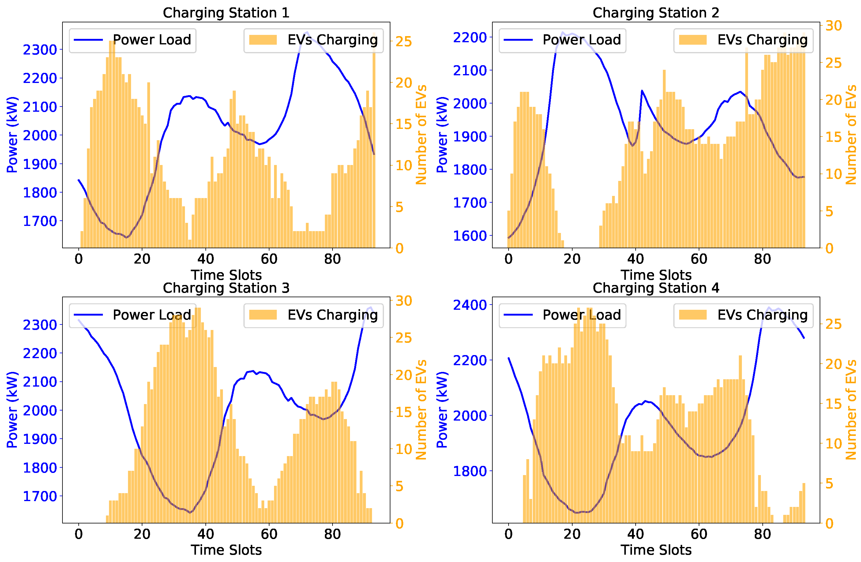
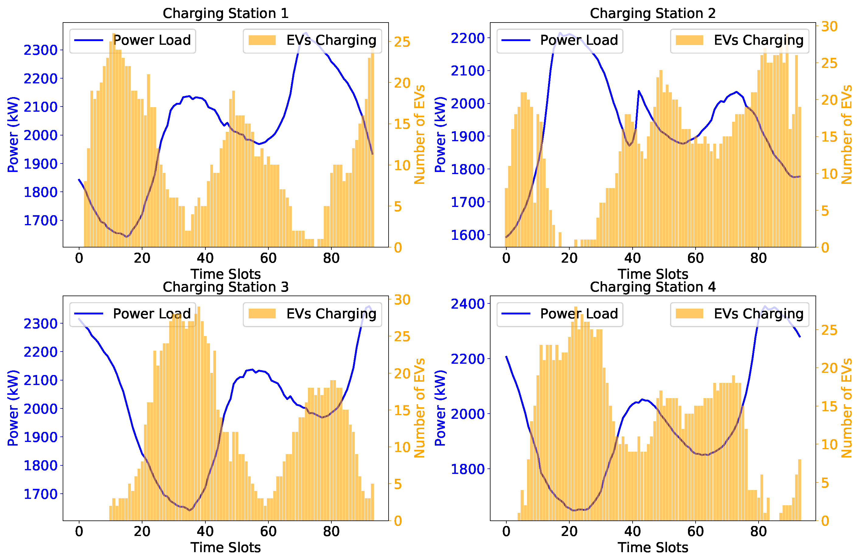
In this study, we first employ the LBMS to guide EV users in selecting charging stations. Therefore, analyzing the EV charging distribution at different time slots across various charging stations is crucial, as it directly reflects whether the proposed station allocation strategy effectively promotes load balancing among distribution networks. Figure 7, Figure 8 and Figure 9 illustrate the distribution of EVs in each charging station at different time slots under the DRL_Space, DRL_Cost, and DRL_Both strategies, respectively, when the number of EVs is set to 1250.

As shown in the figures, the proposed charging station allocation strategy effectively guides users to charging stations with lower loads. Regardless of the specific strategy employed, a consistent trend is observed—when a charging station has a higher load, the number of EVs charging at that station is relatively low, whereas when the station has a lower load, more EVs tend to charge there. This pattern emerges because the LBMS strategy prioritizes recommending charging stations with lower current loads. Through this scheduling mechanism, EV users are directed to stations in less-loaded distribution networks, effectively reducing the load disparity among distribution networks and further enhancing overall load balancing. This trend demonstrates that the LBMS strategy successfully distributes EV charging demand, preventing excessive charging concentration in high-load areas.

However, it is worth noting that although all three figures exhibit a trend toward load balancing, the number of EVs in the same charging station varies across different time slots. This variation primarily stems from the impact of different in-station coordinated charging strategies on EV scheduling. Different strategies not only influence the load fluctuation patterns of charging stations but also have distinct effects on user charging costs. Therefore, in the following analysis, we will further explore the specific impact of different in-station coordinated charging strategies on charging station load and user costs, as well as the influence of varying weight factors on overall system performance.

4.4. Performance of Spatial Load Balancing

To compare the performance of different algorithms in spatial load optimization, we comprehensively evaluate the impact of EV charging on spatial load using the average SLVTPR and the average spatial load standard deviation. Specifically, the calculation of the average SLVTPR is

$$\begin{array}{c}\hfill \overline{\eta }={\displaystyle \frac{1}{T^{tot}}}\sum \eta \left(t\right)\end{array}$$

(26)

$\overline{\eta }$ only reflects the extreme differences among distribution networks, making it difficult to capture the overall load disparity among all distribution networks. Therefore, it is necessary to introduce the average spatial load standard deviation to better show the load differences across all distribution networks. Specifically, the calculation of the average spatial load standard deviation is

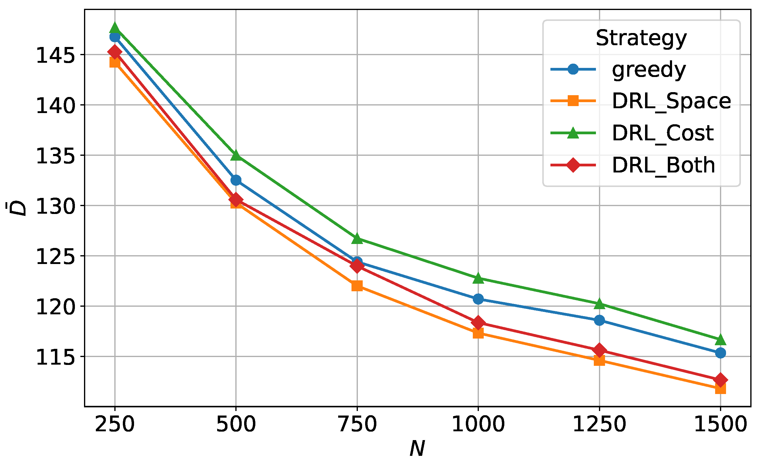
Figure 10 and Figure 11 depict the performance of $\overline{\eta }$ and $\overline{D}$ in the distribution network under different numbers of EVs requesting charging. From these figures, a comparison between the greedy strategy and the DDQN-based strategies under different optimization functions reveals that, although the greedy strategy can achieve spatial load balancing to a certain extent, it is not as effective as the DRL_Space strategy and DRL_Both strategy. This is because the greedy strategy essentially represents an LBMS approach that only considers spatial load balancing. This strategy selects charging stations based on the distribution network load at the time a charging request is submitted. However, due to the delay effect in user travel, by the time the user actually arrives at the charging station, the load at that station may have changed and may no longer be the lowest among all stations. Moreover, the greedy strategy prioritizes immediate charging, which, although facilitating spatial load balancing to a certain extent, does not account for the dynamic evolution of future loads. Consequently, its scheduling performance remains suboptimal and fails to achieve a globally optimal allocation.

$$\begin{array}{c}\hfill \overline{D}={\displaystyle \frac{1}{T^{tot}}}\sum D\left(t\right)\end{array}$$

(27)

where $D\left(t\right)$ is the standard deviation of load among distribution networks at time t.

The DRL_Space strategy and DRL_Both strategy demonstrate better performance in terms of spatial load balancing. Although the DDQN algorithm uses the same charging station allocation strategy as the greedy strategy when assigning charging stations to users, it optimizes the charging power selection based on the base load conditions of the distribution network at the time the user arrives. Under this charging power allocation strategy, the actions taken by the agent lead to a more balanced load across the distribution networks. On the other hand, the DRL_Cost strategy does not consider spatial load balancing in its charging strategy, which results in less effective load balancing compared to the other three strategies.

4.5. Performance of Charging Cost

As the primary participants in the charging process, EV users are primarily concerned with charging costs. Uncoordinated charging can lead to some users charging during periods of high electricity prices, resulting in increased costs. Additionally, certain users may be unable to complete their charging needs within their parking time, leading to “default” situations, where the charging stations must compensate these users, significantly impacting the costs of the charging station as well. Therefore, it is necessary to compare the user charging costs across all charging stations under the four different charging strategies. In this paper, we use the following formula to calculate the total charging cost for EV users:

$$\begin{array}{c}\hfill Cost={\displaystyle \sum _{t=1}^{T^{tot}}}{\displaystyle \sum _{j=1}^M}{N}_{j,t}^c{p}_{j,t}\end{array}$$

(28)

From Figure 12, it is evident that, when comparing the greedy strategy with those based on the DDQN algorithm, the greedy strategy results in the highest user charging costs. This is because the greedy strategy fulfills the user’s charging needs as quickly as possible, neglecting the flexibility users may have during their parking period, which leads to increased charging costs.

In contrast, although the DDQN-based strategy relies on the LBMS strategy during the charging station allocation phase, it fully exploits user charging flexibility in the in-station charging phase. This allows it to dynamically adapt to varying load conditions and electricity price fluctuations, intelligently adjusting charging power to optimize overall charging scheduling. As a result, the user charging costs under the three DDQN algorithms are lower than those under the greedy strategy. However, different reward functions have varying impacts on user charging costs. For the DRL_Space strategy, the agent does not consider information about electricity prices and, therefore, cannot adjust charging power based on the prices at the charging stations. Consequently, the performance in terms of user charging costs is not as favorable as in the other two DDQN algorithms that incorporate cost considerations in their reward functions.

For the DRL_Both strategy, the reward function design includes consideration of the users’ charging costs, which results in lower charging costs compared to the DRL_Space strategy. However, this strategy must balance between minimizing charging costs and the spatial load standard deviation, leading to higher costs relative to the DRL_Cost strategy.

In the case of the DRL_Cost strategy, the input information to the agent consists solely of the charging prices at each time slot. After multiple iterations, the agent selects a charging strategy that minimizes the user’s charging costs. As a result, this reward function yields the lowest user costs.

4.6. Comprehensive Performance of Cost and Spatial Load Balancing

The above results focus on comparing the system performance from the perspective of spatial load balancing or user charging costs, making it difficult to reflect the overall performance of the DDQN algorithm under different optimization functions. To comprehensively evaluate the overall system performance under the three reward functions, we first normalize the charging costs and spatial load standard deviations obtained from the DDQN algorithm with different reward functions using (17). This yields the normalized charging station costs $Cos{t}^{norm}$ and the normalized spatial load standard deviations $D^{norm}$ as

$$\begin{array}{c}\hfill Cos{t}^{norm}={\displaystyle \frac{Cos{t}^{max}-Cos{t}_t}{Cos{t}^{max}-Cos{t}^{min}}}\end{array}$$

(29)

$$\begin{array}{c}\hfill D^{norm}={\displaystyle \frac{D^{max}-D_t}{D^{max}-D^{min}}}\end{array}$$

(30)

Then, by adding $Cos{t}^{norm}$ and $D^{norm}$, we obtain the normalized total result $Tota{l}^{norm}$, which comprehensively considers both factors. The corresponding expression is

$$\begin{array}{c}\hfill Tota{l}^{norm}=Cos{t}^{norm}+D^{norm}\end{array}$$

(31)

For example, when the number of EVs is 1000, the charging costs under the DRL_Space, DRL_Cost, and DRL_Both strategies are 2620.19, 2594.48, and 2611.23, respectively, and the corresponding spatial load standard deviations are 117.32, 122.78, and 118.36, respectively. Using (29) and (30), the $Cos{t}^{norm}$ values under the three reward functions are 0, 1, and 0.35, and the $D^{norm}$ values are 1, 0, and 0.81, respectively. Summing them up using (31), the $Tota{l}^{norm}$ values are 1, 1, and 1.16. Similarly, the total normalized results can be obtained for other EV numbers, comprehensively considering both factors.

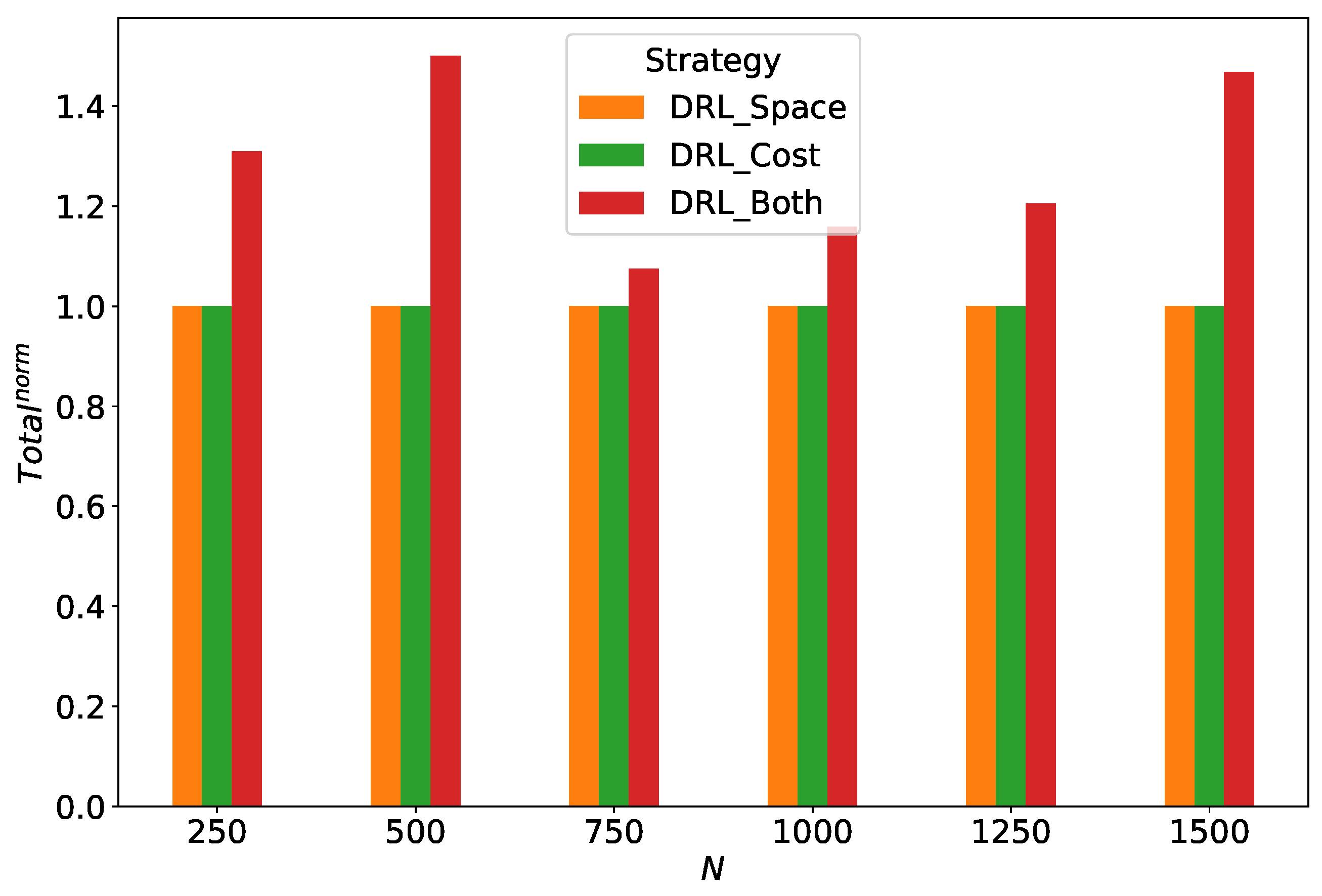
As shown in Figure 13, both the DRL_Space strategy and DRL_Cost strategy have a $Tota{l}^{norm}$ value of 1. Under the DRL_Cost strategy, this approach selects a charging power that minimizes the charging price for EVs, disregarding the load distribution across the power grids. In contrast, the DRL_Space strategy prioritizes charging power that balances the load among the power grids, overlooking the users’ charging costs. Both strategies focus on only one aspect, which limits the overall performance of the algorithm.

However, under the DRL_Both strategy, $Tota{l}^{norm}$ is the highest. This is because, this strategy considers both user charging costs and load balancing when selecting the charging power at each time slot. After balancing these two factors, the strategy selects actions that can both reduce user charging costs and minimize the load disparity among distribution networks. Therefore, this strategy achieves the highest reward value, and the system’s overall performance is the most balanced.

Table 2. Impact of different weights on system performance with 1250 EVs.

Different Weight	$\overline{\mathit{\eta }}$	$\overline{\mathit{D}}$	Cost
$\alpha =0,\beta =1$	89.23%	114.62	3480.74
$\alpha =0.3,\beta =0.7$	89.15%	114.93	3474.34
$\alpha =0.5,\beta =0.5$	89.03%	115.62	3470.37
$\alpha =0.7,\beta =0.3$	89.01%	116.63	3466.26
$\alpha =1,\beta =0$	88.72%	120.24	3453.79

presents the impact of different weights on system performance when there are 1250 EVs. As observed from the table, with the increase in $\alpha$ (user charging cost weight), user charging costs gradually decrease, while the spatial load standard deviation increases. This happens because as $\alpha$ increases, the agent prioritizes minimizing user charging costs during optimization, with less emphasis on balancing the load across the distribution networks. Therefore, when $\alpha$ = 1, the agent fully focuses on optimizing user charging costs, leading to the highest charging cost and the poorest load balancing.

4.7. Performance of Weight Factor Sensitivity

Conversely, as $\beta$ (load balancing weight) increases, the agent focuses more on balancing the load across the distribution networks during optimization. With the increase in $\beta$, user charging costs gradually rise, while the spatial load standard deviation decreases. This is because, when the agent places more emphasis on balancing the load among the distribution networks, it actively schedules some users to charge during time periods with more uneven spatial load, thereby achieving load balancing among the distribution networks. However, this adjustment may lead to higher charging costs for some users. Consequently, when $\beta$ is high (corresponding to higher charging costs in the table), the agent’s scheduling strategy can significantly reduce the spatial load standard deviation.

The above analysis demonstrates the varying impacts of different weights on system performance, but it is not straightforward to select a single optimal strategy. Therefore, a comprehensive evaluation of the DDQN algorithm’s performance under different weights is necessary. In this section, we continue to apply the normalization method from Section 4.6 to the results obtained under different weights, and the outcomes are shown in Figure 14.

Figure 14 illustrates the impact of different weights on overall system performance under varying numbers of vehicles. From the figure, it is evident that when $\alpha =1$ or $\alpha =0$, the system’s overall performance is the worst. In both of these cases, although the optimization objectives are individually achieved at their optimal values, the failure to account for the other factor simultaneously leads to a decline in overall system performance. However, when $\alpha =0.3$ or $\alpha =0.7$, the system’s overall performance is significantly better than when considering only a single factor. This is because, during the optimization process, the introduction of an additional factor forces the agent to balance both optimization goals. However, due to the weighting scheme, the agent inevitably favors one aspect over the other. Thus, despite some improvements, the optimal balance has not been fully achieved.

When $\alpha =0.5$, the system achieves the best overall performance across different vehicle numbers. This is because, in this configuration, the system does not prioritize either user charging costs or load balancing across the distribution networks but seeks a balance between the two. Although, in this case, the user charging costs and spatial load standard deviation are not optimal, they represent the most balanced solution, indicating that the proposed strategy is a well-balanced optimization approach.

In summary, the trade-off between $\alpha$ and $\beta$ weights directly influences the system’s optimization objectives. When $\alpha$ is higher, the system tends to prioritize minimizing user charging costs, which may result in imbalanced load distribution; whereas when $\beta$ is higher, the system focuses more on optimizing load balancing across the distribution networks, which may lead to sacrificing some user charging cost efficiency. When $\alpha$ and $\beta$ are equal, the system exhibits the strongest overall performance. Therefore, a reasonable setting of the $\alpha$ and $\beta$ weight ratio can achieve a better balance between load balancing and user cost optimization.

4.8. The Impact of Different User Participation Levels on System Performance

In practical applications, the level of user participation plays a crucial role in charging station scheduling and the overall performance of the system. Not all users strictly follow the scheduling center’s recommendations when selecting a charging station; instead, they may make decisions based on personal preferences. Such random selection behavior can lead to imbalanced load distribution across the power grid and increase the overall charging cost. Consequently, the degree of user participation directly determines whether a charging strategy can effectively optimize grid load distribution while minimizing charging costs. To evaluate this impact, Figure 15, Figure 16, Figure 17 and Figure 18 illustrate the effects of different user participation levels on system performance, considering a total of 1000 charging requests. These figures provide an intuitive understanding of how varying degrees of user participation influence load balancing and charging costs, thereby enhancing the comprehension of system optimization strategies.

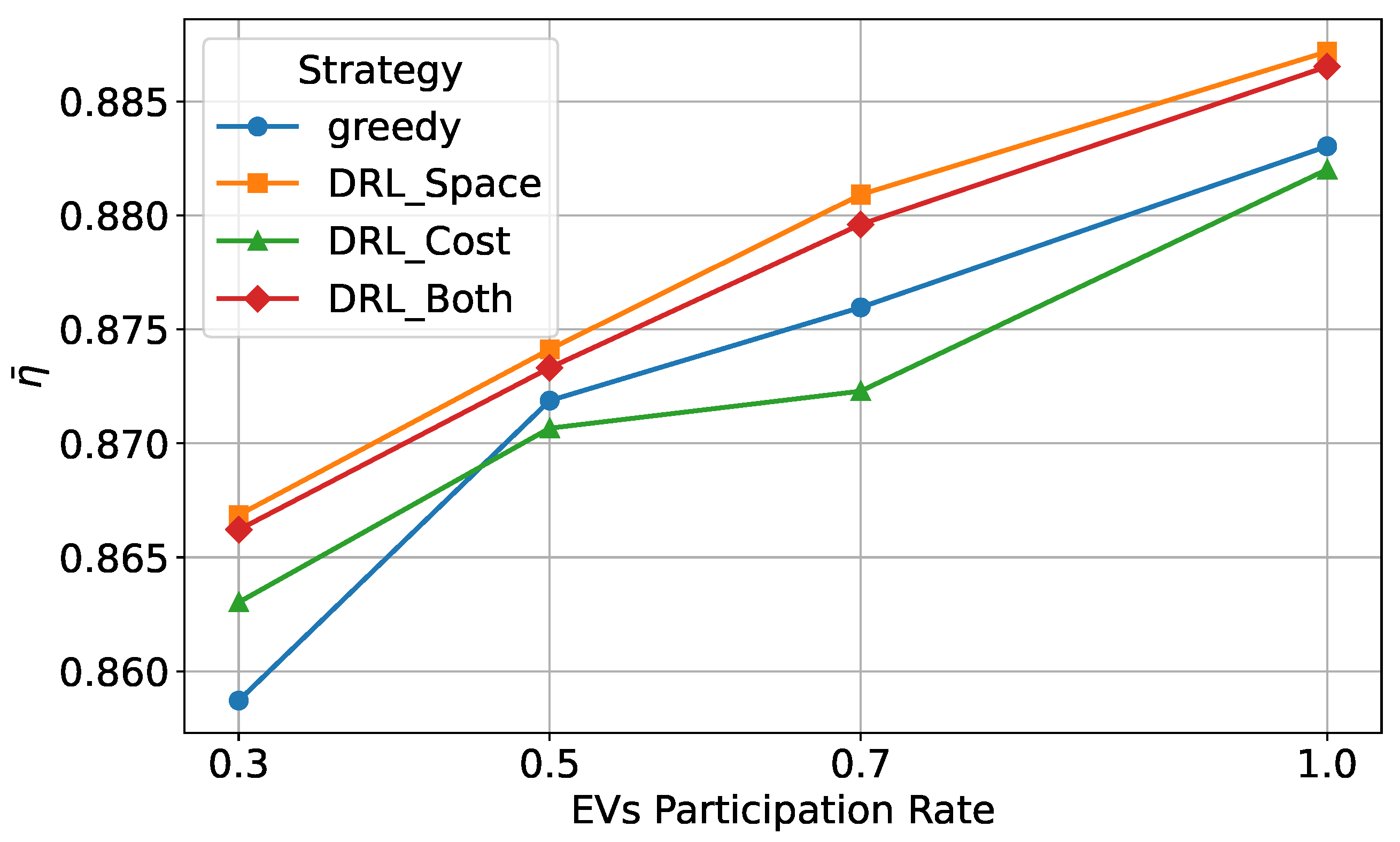
From Figure 15, it can be observed that as the EV user participation rate increases, the SLVTPR values for all strategies exhibit an upward trend, indicating that users following the LBMS-based charging station recommendation strategy can significantly improve load balancing. Among all strategies, DRL_Space and DRL_Both demonstrate the best performance. This is because DRL_Space focuses specifically on load balancing, ensuring a more even distribution of load among charging stations. Meanwhile, DRL_Both considers both load balancing and charging costs, optimizing load distribution while maintaining economic efficiency. As a result, DRL_Both can still achieve effective load balancing; however, since it simultaneously accounts for both user cost and load balancing, its spatial load balancing performance is slightly inferior to that of DRL_Space.

In contrast, at low user participation levels, the greedy strategy exhibits poor load balancing performance, even lower than that of DRL_Cost. This is because the greedy strategy selects charging stations solely based on the lowest current load, without considering future load variations, which can lead to station overloading. However, as user participation increases, the load balancing performance of the greedy strategy gradually surpasses that of DRL_Cost, indicating that when a greater number of users opt for charging stations with lower loads, the effectiveness of the greedy strategy in achieving load balancing improves. Nevertheless, since DRL_Cost primarily optimizes charging costs, its load balancing performance is slightly inferior to other methods at higher user participation levels.

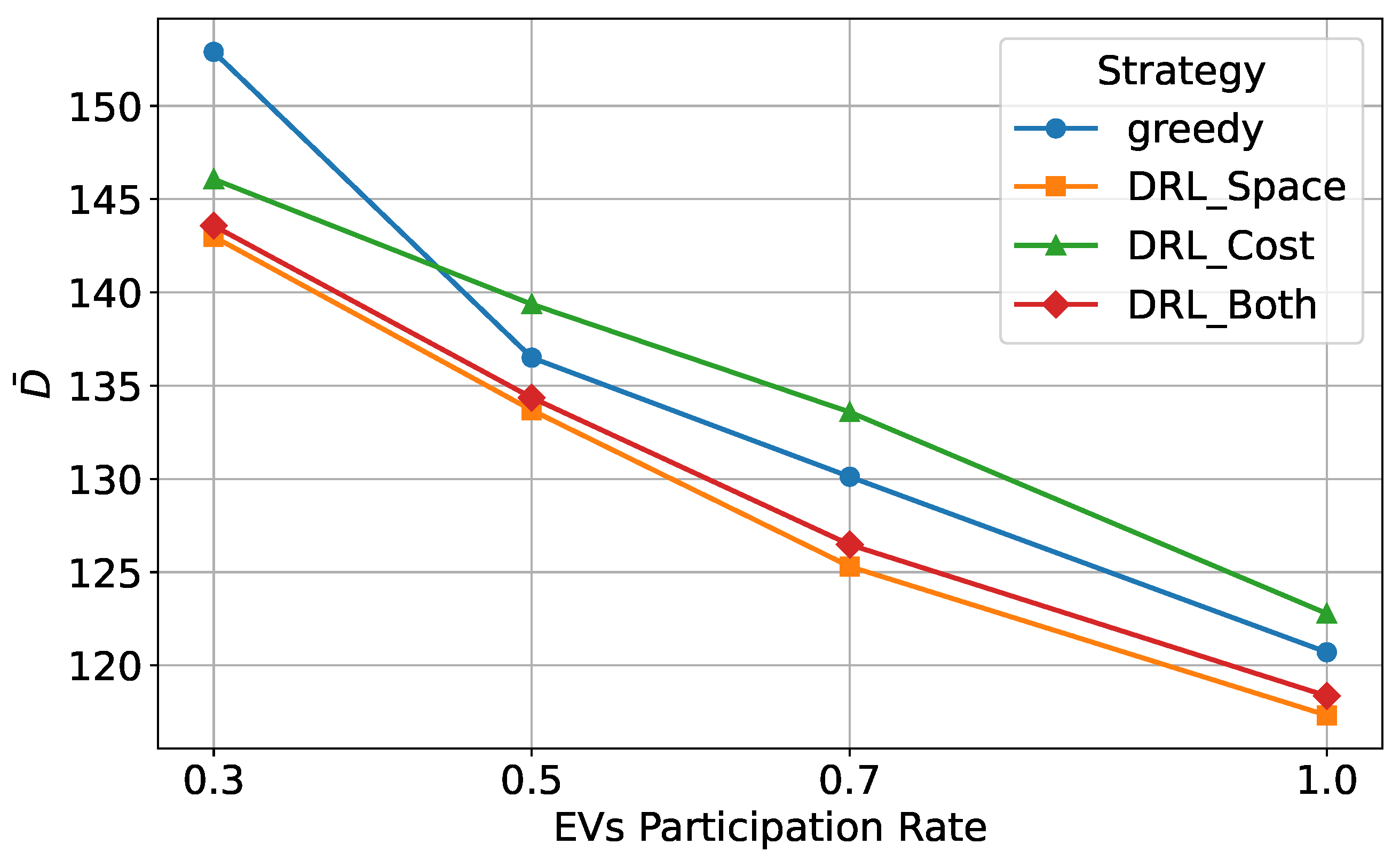
Figure 16 illustrates the spatial load standard deviation under different levels of user participation. From the figure, it can be observed that as user participation increases, the spatial load standard deviation decreases across all strategies, indicating that higher user participation contributes to improved load balancing. Among all strategies, DRL_Space and DRL_Both exhibit the lowest standard deviation, demonstrating their superior ability to balance loads effectively, particularly at high user participation levels. The greedy strategy shows the highest standard deviation at low user participation levels, indicating that it causes significant fluctuations in load distribution. Although DRL_Cost achieves better load balancing than the greedy strategy at lower user participation levels, its load balancing performance remains inferior to that of the other strategies as user participation further increases.

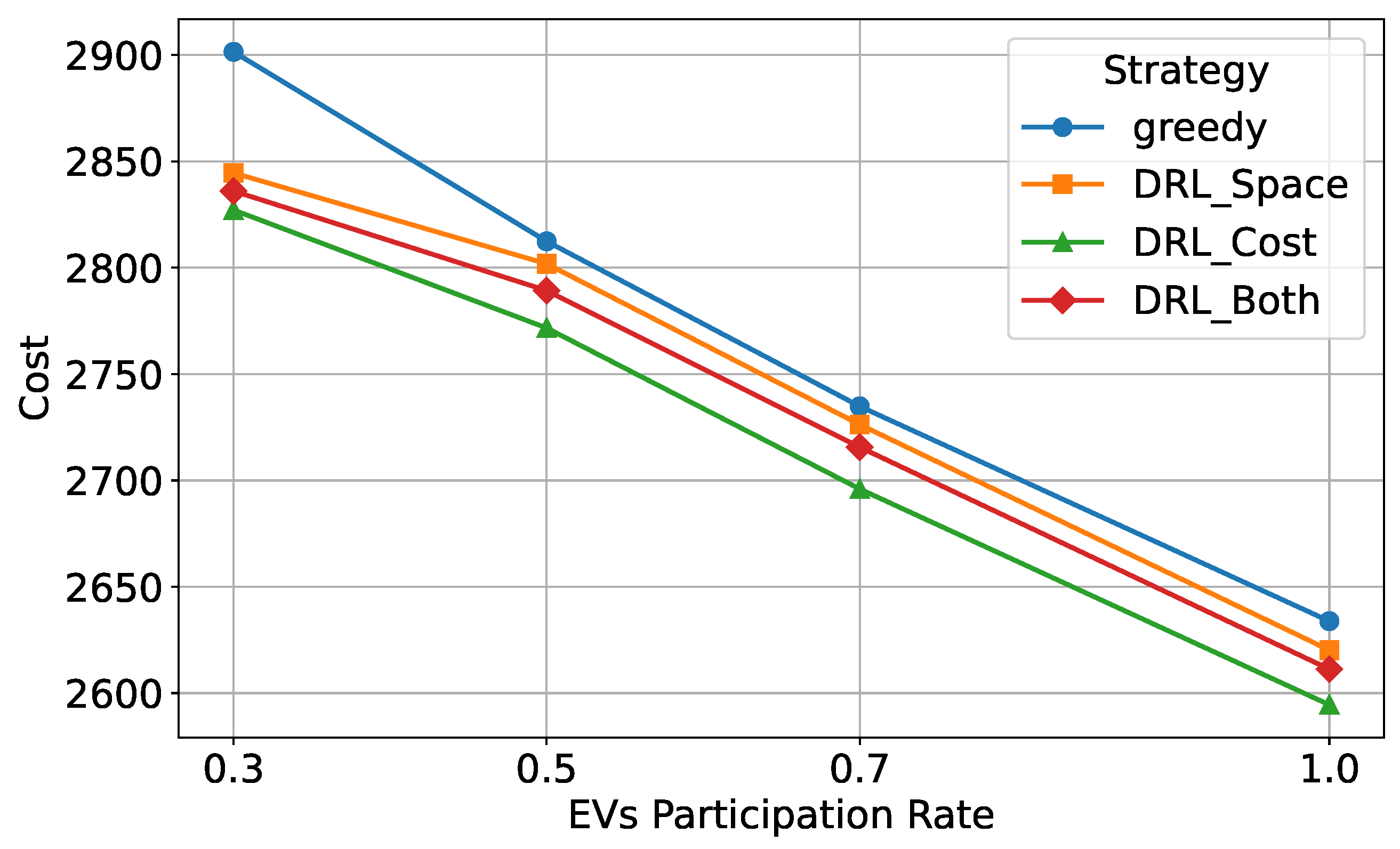
Figure 17 illustrates the total charging cost under different user participation levels. As user participation increases, the overall charging cost decreases, indicating that the LBMS-based charging station recommendation strategy generally enables users to access lower electricity prices, thereby effectively reducing charging costs. Among all strategies, DRL_Cost consistently achieves the lowest charging cost, as its primary optimization objective is to minimize user costs. Even at low participation levels, this strategy effectively reduces costs, demonstrating strong economic optimization capabilities. DRL_Both, as a comprehensive optimization strategy, performs slightly worse than DRL_Cost in cost reduction but outperforms DRL_Space, indicating that it maintains a balance between cost reduction and load balancing, ensuring overall system stability. In contrast, DRL_Space focuses more on load balancing and gives less consideration to price optimization, resulting in higher costs than DRL_Both and DRL_Cost, though it still significantly outperforms the greedy strategy. The greedy strategy incurs the highest charging cost, especially at low user participation levels, where costs are significantly higher than those of other strategies. This is because the greedy approach selects the charging station with the lowest current load without considering electricity prices or future load variations, leading to station overload and increased charging costs. As a result, DRL_Cost provides the best economic performance, DRL_Both achieves a trade-off between cost control and load balancing, while DRL_Space and the greedy strategy result in relatively higher charging costs.

Figure 18 further illustrates the overall system performance of different optimization strategies. Across all user participation levels, DRL_Both achieves the highest overall performance score, indicating that this strategy effectively balances load distribution and charging costs, ensuring maximum system benefits. In comparison, DRL_Space and DRL_Cost perform well in their respective optimization objectives but fall slightly short of DRL_Both in overall performance. DRL_Space excels in load balancing, but since it does not explicitly optimize charging costs, its overall system performance is slightly lower than that of DRL_Both. On the other hand, DRL_Cost demonstrates the best performance in controlling charging costs but does not sufficiently address load balancing. Therefore, its overall system performance is also inferior to that of DRL_Both.

5. Conclusions and Future Work

The travel patterns and charging demands of EV users are characterized by significant uncertainty, and without proper coordination, this can lead to increased user charging costs and jeopardize the safe operation of the distribution grids. In contrast, if the selection of charging stations and charging behaviors within the stations is properly coordinated, it is possible to effectively control user charging costs and reduce the load imbalance across the distribution grids. In this paper, DRL-based optimization strategies for EV charging are proposed, aiming to minimize user charging costs while achieving load balancing in the distribution grids. By employing a load balancing matching strategy to guide users to the charging stations with the lowest load and integrating the DDQN algorithm to optimize the orderly charging process within the stations, this strategy effectively addresses the uncertainty in user travel and charging demands, significantly reducing charging costs and enhancing the safety of distribution grids.

Simulation results indicate that, compared to the traditional LBMS algorithm, the proposed DRL approaches excel in controlling charging costs and optimizing load balancing across the grids. Specifically, when the reward function focuses on minimizing user charging costs, the strategy effectively reduces user costs; when the reward function aims to minimize the load imbalance in the distribution grids, it significantly improves load balancing. Furthermore, when the reward function considers both user charging costs and grids’ load balancing, it achieves an optimal balance between the two. Additionally, the strategy demonstrates robust performance across various levels of user participation, effectively minimizing user costs and optimizing grids’ load balance regardless of the participation rate, illustrating the strategy’s ability to handle dynamic and uncertain environments effectively.

The model proposed in this paper can be deployed in a large-scale urban environment, in which a centralized dispatching unit can be established to supervise the user’s choice of charging stations and the dispatching of charging stations. When a user needs to charge his EV, the dispatching center can adopt the proposed charging station allocation strategy to recommend a suitable charging station for the EV. When the user arrives at the charging station, the dispatching center will send the distribution network information to the station. The charging station can combine this information with its own charging price and use the DRL model proposed in this study to dynamically adjust the weight ratio according to the needs of the charging station and the power grid to achieve the charging power allocation for the EV. In addition, this strategy is not only applicable to EV charging networks, but can also be applied to other complex scenarios, such as energy management (such as virtual power plants, distributed energy scheduling) and resource allocation (such as logistics optimization, fleet scheduling), providing theoretical support and practical guidance for solving dynamic optimization problems in various fields.

In future work, the proposed strategy can be further enhanced in the following three aspects:

1.

V2G technology could be incorporated into future research, potentially further reducing users’ charging costs and enhancing load balancing across distribution networks.

2.

Future research could explore the impact of highly dynamic conditions, such as fluctuations in traffic flow or surges in user demand, on the performance of the system.

3.

The time-of-use electricity prices used in this paper are fixed. Future research can incorporate dynamic pricing to further explore the impact of price uncertainty on system performance.