Slow but Steady: Assessing the Benefits of Slow Public EV Charging Infrastructure in Metropolitan Areas

Abstract

Vehicle-grid integration (VGI) is critical for the future of electric power systems, with decarbonization targets anticipating millions of electric vehicles (EVs) by 2030. As EV adoption grows, charging demand—particularly during peak hours in cities—may place significant pressure on the electrical grid. Charging at high power, especially during the evening when most EVs are parked in residential areas, can lead to grid instability and increased costs. One promising solution is to leverage long-duration, low-power charging, which can align with typical user behavior and improve grid compatibility. This paper delves into how public slow charging stations (<7.4 kW) in metropolitan residential areas can alleviate grid pressures while fostering a host of additional benefits. We show that, with respect to a reference (22 kW infrastructure), such stations can increase EV user satisfaction by up to 20%, decrease grid costs by 40% owing to a peak load reduction of 10 to 55%, and provide six times the flexibility for energy markets. Cities can overcome the limitation of private garage scarcity with this charging approach, thus fostering the transition to EVs.

1. Introduction

The electrification of transportation is one of the most significant transformations in energy systems, driven by the dual imperatives of reducing greenhouse gas emissions and improving the urban air quality. Electric vehicles (EVs) have emerged as a key pillar of this transition, with sales around 15 million EV yearly in the world, with a global sales share of battery electric vehicles (BEVs) and plug-in hybrid electric vehicles (PHEV) of 18% in 2023 (38% in China and 21% in Europe) [1]. However, this rapid adoption poses challenges for electricity grids, particularly in urban areas, where charging demand may coincide with peak electricity usage, straining grid infrastructure and increasing costs. The role of innovative charging strategies in addressing these challenges has been the central focus of recent research [2]. Charging infrastructure is a crucial enabler of this transition. While fast-charging stations provide convenience for long-distance travel and commercial fleets, they are not always the most efficient solution for urban areas. In contrast, standard AC public charging is typically outperformed by work and home charging, where they are available [3]. Premising that the first target must be reducing the number of cars and car trip in metropolitan areas (and there are dozens of possible solutions [4]), in dense metropolitan environments, space constraints, high electricity demand during peak hours, and the need for cost-effective solutions make low-power, very slow charging stations practical [1,5]. For slow charging, literature usually considers power rates equal to or lower than 7.4 kW (Level 1 or 2 below or equal to 230 V, 32 A, 1-phase systems). Public slow charging matches well with residential or work charging patterns, where vehicles remain parked for extended periods of time. In particular, it becomes essential in the absence of a private garage [3]. By aligning charging with these patterns, grid operators can optimize electricity use, reduce peak demand, and improve overall system efficiency. Recent studies have highlighted the benefits of slow charging in urban settings. For example, ref. [6] demonstrated that low-power charging reduces the peak loads on the grid by distributing the demand more evenly throughout the day. Even in this case, surveys suggest that deploying distributed charging infrastructure in residential areas enhances accessibility, particularly for users without private garages or driveways [7]. Even if policymakers and urban planners are increasingly recognizing the importance of these benefits in designing sustainable cities, the role of slow chargers in cities is underexplored or often sidelined in policy discussions. Nonetheless, electric mobility diffusion is particularly important in cities since it can reduce local pollution levels, which are typically high.

If the prevailing EV charging behaviors are disregarded in the urban planning phase, obstacles to EV adoption in cities may arise. All the scenarios to 2030 show that charging at home will represent around 50% of charging in 2030, followed by charging at work (15–25%). The charging mode distribution, as proposed in [8], is presented in Figure 1 B2C charging (or charging at the destination) means charging at EVSE provided by businesses offering other services (e.g., in the mall parking), while public charging means charging at EV supply equipment (EVSE) typically present on public roads or parking lots. Public charging appears to have, generally, a marginal role (10–20%) [8,9,10,11].

If residential charging is and will be the preferred solution, this confirms that the lack of private garages (or private parking lots) could hamper EV diffusion. This is particularly relevant in large cities. An analysis by a real estate online agency based on 1.3 million households highlighted that 40% of households in Italy can host private home charging, but this percentage is halved in municipalities with more than 200,000 citizens due to the lack of car garages [12]. The distribution of households with a private garage in Italy is shown in Figure 2, which compares the overall situation with that of large cities. As can be seen, 67% of large cities in Italy feature less than 20% of households with private car garages. Considering all municipalities, 95% of them feature more than 20% of households with private car garages.

Therefore, EV diffusion can be hindered, where the reduction of internal combustion engine vehicles would be most beneficial. In this context (representing 16% of the Italian population, as already shown), there is possibly room for exploiting slow charging over long stops as a key VGI technique for scaling up EV adoption without jeopardizing the distribution grid.

In this work, slow public charging is investigated as a solution for the early adoption (2025 to the early 2030s) of EVs in large cities. To do so, public EV charging in cities should be affordable (it should substitute residential charging, which is hampered) and integrated with the distribution grid and power system. As observed, we can foresee several advantages, such as a lower peak power demand and high compatibility with long-duration stops. Despite these advantages, implementing slow charging systems requires careful planning to balance user satisfaction and grid efficiency. Users expect reliable access to charging points and sufficient power to meet their needs. For instance, delays in charging availability can impact user confidence and lead to dissatisfaction. This paper addresses these challenges by presenting a comprehensive methodology for evaluating the techno-economic benefits of slow charging stations in metropolitan residential areas. Our analysis focuses on three key dimensions: user satisfaction, grid cost reductions, and flexibility for electricity markets. A comparative analysis between two charging stations is proposed, assessing the differential benefits of implementing a standard charging station featuring EV supply equipment (EVSE) with 22 kW AC charging capability vs. a slow station featuring EVSE with 7.4 kW of nominal power per pole and an overall limit for power withdrawn from the grid. By extending our findings to a national scale, we aim to provide actionable insights for policymakers, grid operators, and stakeholders to enhance the urban EV charging infrastructure.

The remainder of this paper is structured as follows. Section 2 describes the proposed methodology for building charging profiles and the comparative cost-benefit analysis. Section 3 presents the case studies considered. Section 4 presents the results in terms of user satisfaction, impact on the grid, and flexibility provision. Section 5 presents the conclusions.

2. Proposed Methodology

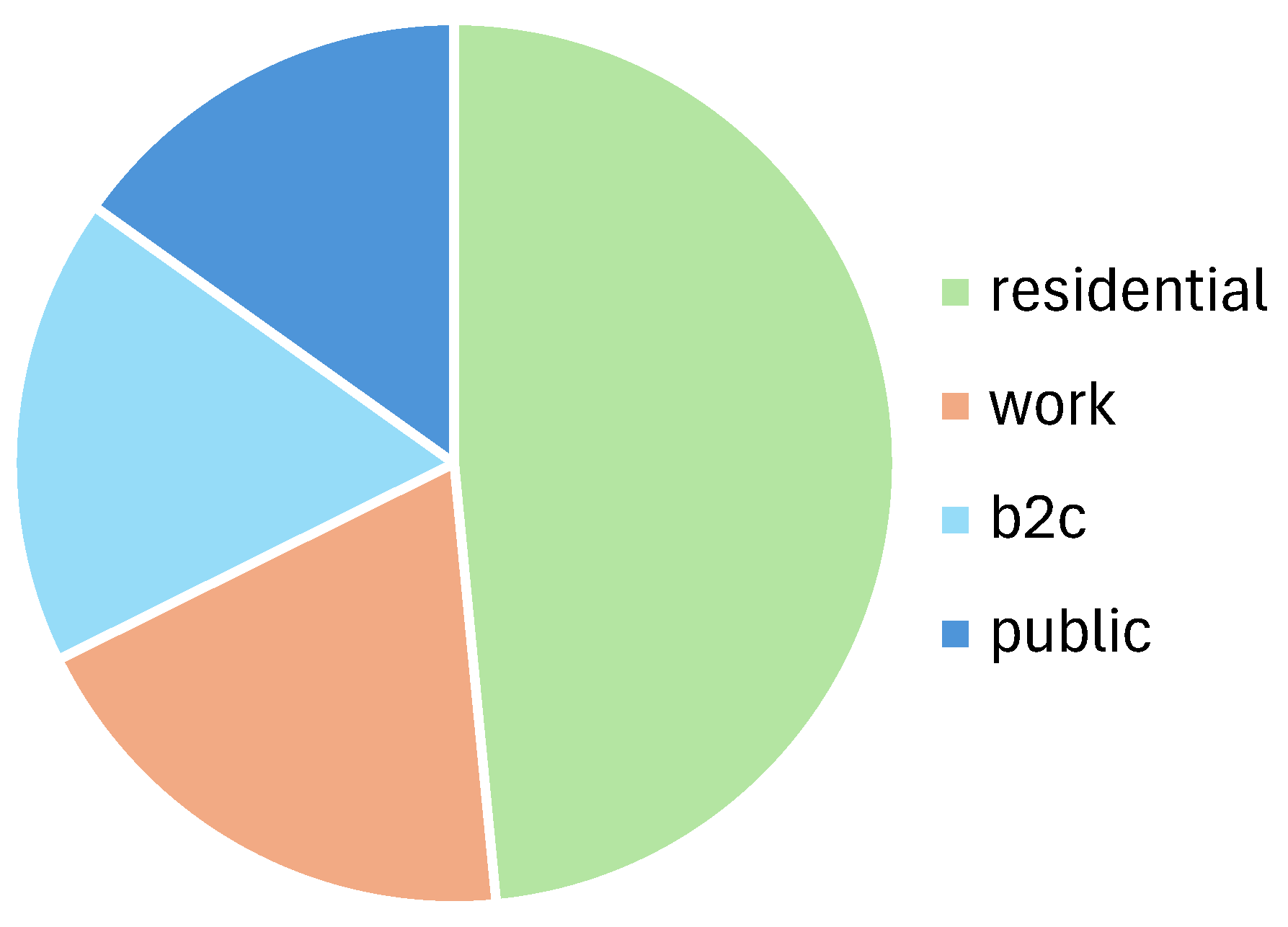
The proposed approach aims to analyze the benefits of slow public charging (i.e., EVSE power = 7.4 kW) in the residential areas of large cities. The study is performed within the Italian framework. Therefore, a city is considered large if it has 200,000 citizens or more. Fifteen cities are included in the definition, with an overall population of 9.8 million people (16% of the Italian population). In these cities, as seen before, there is a serious obstacle to residential charging: the lack of private garages or private parking. Public charging can cope with this only if it can adapt to the residential charging needs. Slow, mainly nightly charging is selected as a possible solution and is analyzed in the following sections. All the simulations described have been performed on a standard personal computer with a 1.3 GHz CPU and 16 GB of RAM.

2.1. Development of Charging Profiles

To evaluate the impact of slow charging on user satisfaction and grid performance, we developed a simulation model to generate realistic charging profiles for a fleet of EVs. The model incorporates the entry and exit profiles, vehicle specifications, and EVSE constraints. The entry and exit profiles are updated from a previous statistical review of sources [8]. The investigated sources are scientific and institutional sources. Study [13] compared controlled and uncontrolled charging in residential premises in a future scenario with high EV penetration. A report [14] shows residential charging patterns in a UK study of EV early adopters. In [15], the authors elaborated on real-world data from the Netherlands to estimate the impact of residential charging in 2030. Similar studies have been conducted in England [16] and the US based on travel surveys [17]. All the cited studies elaborate on today’s data or surveys to estimate future scenarios. Indeed, today’s data per se cannot represent a future mature market [18]. The adopted entry/exit profiles represent the average of the reported sources. The profiles are presented in Figure 3. They represent the expected entry and exit for charging in a residential area, either in the case of private or public infrastructure. Among the four analyzed typical days (working/weekend day, cold/warm season), we present the profiles for a working day in the cold season. As can be seen, the peak of entry is at the end of business (EoB), charging is typically during night hours, and the peak of exits is in the first morning.

Regarding the charging EV fleet, the breakdown presented in

Table 1. Distribution and data of the EV fleet in 2030.

Segment	Capacity (kWh)	AC Charging Power (kW)	Diffusion
A	45	7.4	35%
B	55	7.4	15%
C	65	11	22%
D	80	22	8%
E+	100	22	4%
PHEV_A-B-C	12	3.7	14%
PHEV-D-E+	15	7.4	2%

is proposed, based on the Italian car industry association [19] and a statistical analysis of available EVs [20]. It reflects the expected relative diffusion between BEV and PHEV in a 2030 scenario, the car segments for each group, the maximum chargeable power, and the battery nominal energy.

A Python 3.13 routine simulates the arrival and departure times of vehicles at residential charging stations starting from the previously shown distribution, as well as their energy requirements based on the battery size, initial state of charge (SoC), and target SoC. Two intervals are defined for the initial (30–60%) and target SoC (80–100%) of approaching EVs, and the value for each EV is randomly selected. The charging station has a fixed number of charging points.

The yearly simulation begins by selecting the number N of EVs per day. N is selected to be coherent with the expectations of EV and EVSE diffusion to 2030 from the Italian Energy and Climate Plan [21]. To each vehicle, the routine assigns the entry and exit hour, the initial and target SoC, and a segment (with all related data). The number N of approaching vehicles is typically greater than the number of charging spots. Therefore, it is not guaranteed that an approaching EV can start charging, and the EV user can satisfy its charging needs. A set of satisfaction challenges is proposed in Section 2.2.

Once an EV is connected, a presence profile is generated based on the entry and exit (see also Figure 4). Based on the charging power and the initial vs. target SoC, the charging, not charging, and power profiles are developed. $P_i$ is by default equal to the segment’s AC charging power of the considered EV, as per Table 1. The charge duration can be less than or equal to the stop duration. The key times of each stop $i$ are the beginning of the stop ($T_{in,i}$), the end of charging (${EoC}_i$), the charge duration ($\Delta T_i$) and the end of the stop ($T_{fin,i}$), which may be perhaps equal to $Eo{C}_i$.

It is worth noting that, in case a fee for parking after the end of charging exists, the presence array is modified, and $T_{fin,i}$ occurs 1 h after ${EoC}_i$. This is to simulate the behavior of a car user that is not willing to pay the fee for overparking. Figure 5 exemplifies a stop that is updated to avoid overparking fee. Initially, the EV user aimed to connect the EV at 7 a.m. and depart at 6 p.m. Actually, the ${EoC}_i$ occurred at 2 p.m. and $T_{fin,i}$ is anticipated at 3 p.m.

The outputs from this simulation were used to construct aggregate charging profiles for entire neighborhoods, which are critical for assessing their impact on the local grid. For instance, weekday profiles for urban residential areas exhibit clustered demand during evening hours, while weekend profiles spread out the energy requirements over longer durations, reflecting differences in user behavior. To better quantify energy and power results, the overall charged energy is computed, as well as the average power profile for each analyzed case. Additionally, the occupancy ratio (OR) [22] of the charging station is computed as follows.

$$OR\left(\%\right)={\displaystyle \frac{E_{ch}}{P_{EVSE}\times N_{EVSE}\times 8760}}$$

(1)

where $E_{ch}$ is the yearly charged energy in the station in kWh, $P_{EVSE}$ is the nominal power of a charging pole in kW, $N_{EVSE}$ is the number of charging poles deployed in the charging station, and 8760 are the hours in a standard calendar year (we do not consider a leap year). We propose that the charging service is sold for 0.50 €/kWh [23]. This is a slightly lower value with respect to today’s average charging fees in Italy (see

Table 2. EV public AC charging prices in Italy.

Denomination	Price (€/kWh)	Notes
Regulatory investigation (2018)	0.50	Upper price of public AC charging as per an analysis by the national regulatory authority [24]
Maximum commercial price (2025)	0.65	Max average price detected by [23] for public AC charging
Minimum commercial price (2025)	0.50	Min average price detected by [23] for public AC charging
Proposed price	0.50	Low price scenario assumed for the future

), justified by a possible scale economy in the future and by the provision of slow service.

By capturing these detailed patterns, the simulation enables a more nuanced understanding of how slow charging can reduce the burden on the distribution grid and on the power system without compromising user satisfaction.

2.2. Satisfaction Challenges: Evaluating User Satisfaction

User satisfaction in the context of EV charging reflects the reliability and adequacy of the service provided. A set of three challenges is developed to define how many of the typical users (represented by the entry and exit profiles shown in Figure 3) can answer their charging demand with each of the charging infrastructures/modes.

The first key factor is intrinsic capability of the charging mode of satisfying the charging need. This challenge sums two sub-challenges.

• Can the charging mode provide enough energy to reach target SoC within $T_{\mathit{fin},i}$?
• In case of presence of a fee for parking after the end of charging, is the $Eo{C}_i$ occurring outside the nighttime? Indeed, one will not select a charging spot overnight if it implies either disconnection and displacement during the night or the payment of a fee additional to the charging cost.

The second challenge concerns finding a spare charging spot. Indeed, each charging station features a finite number of charging spots. In case all of them are occupied by other vehicles at $T_{in,i}$ (first-come first-served), they oblige the EV user to look for a different station.

The third challenge assesses if any limitation on the whole charging station can prevent reaching target SoC (this challenge is additional with respect to the first one). Indeed, some charging stations present an overall limitation on power withdrawal. In case it is hit, the delivered power to each charging point is reduced proportionally. This can hamper the reach of target SoC in due time.

2.3. Grid Cost Reduction: Evaluating Benefits from Rational Use of Distribution Network

Does slow charging allow to respond to the energy demand with reduced grid costs? To answer this question, we consider the overall power profiles for the charging station obtained from the simulations. Grid cost reductions arise from reduced peak power withdrawn, as slow charging stations distribute energy consumption more evenly over time. For instance, by shifting charging loads to off-peak hours, these systems alleviate pressure on the grid and defer costly infrastructure upgrades. To quantify the possible variation of distribution grid costs by different EV charging strategies, leading to different peak power, we use as a proxy two electricity tariff components, also reported in

Table 3. Grid costs.

Component	Value	Computation
Connection cost (una tantum)	75 €/kW	Multiply the fee by the maximum withdrawn power over lifetime.
Distribution grid costs (yearly)	31.4 €/kW/year (=2.61 €/kW/month)	Multiply the monthly fee by the peak monthly withdrawn power.

.

• We consider the connection costs of an electric consumer, paid upfront in case of a new connection, expressed in €/kW. In Italy, these are updated every year by the National Regulatory Authority (NRA) [25]. These costs are included in the results considering the global maximum power withdrawal as obtained in the simulations. Indeed, a firm connection is sized at the overall peak.
• Then, we consider the tariff component related to distribution. This is paid within the electricity bill, in the grid costs, usually in €/kW/period. In Italy, the distribution tariff is paid (by customers with peak power larger than 50 kW) in €/kW/month on the maximum withdrawn power in the relevant period. The tariff is updated periodically by the NRA [26]. We consider the monthly peak power as obtained by the simulations to evaluate these costs.

The tariff is, in principle, cost-reflective [26], meaning that these fees represent the average cost that the network faces for an additional user with that power demand. Therefore, the connection and operation costs are used to compare the impact on the grids of different charging configurations. For the lifetime analysis, a 3% discount rate is considered, and 20 years of horizon.

2.4. Smart Charging: Evaluating Benefits from Flexibility Provision by EV with No-Harm Approach

Lastly, market flexibility is quantified as the capacity of the system to modulate the charging power in response to real-time grid demands. Flexibility measures the total energy that can be shifted to support ancillary services or balance the supply and demand during critical periods. We consider the “no-harm approach” already presented in [6] to estimate the available flexibility during EV charging, potentially exploitable by the system: an EV can provide flexibility until it reaches a SoC at $T_{fin,i}$ that is greater than or equal to the target SoC. The provided flexibility is estimated from the performed simulations as follows. Each car can provide flexibility if its stop duration is sufficient to reach the target SoC from the initial SoC at ${EoC}_i$, before $T_{fin,i}$. This is the case for the top and mid charts of Figure 4 where, indeed, there are non-null values in the NOT charging array. In this case, the EV can reduce (up to zero) the withdrawn power during the charging hours, thus providing an upward flexibility. In the next hours, the car could charge more than the target SoC, thus increasing the withdrawal (with respect to zero) and providing downward flexibility. Both energy and power margins must be computed to assess the flexibility. Figure 6 better explains the approach with an example. Considering a car stopping for 6 h and reaching the target SoC at the end of hour 3 (${EoC}_i$), the car charges for the first three hours at $P_i$, then remains parked with no withdrawal from hour 4 to 6 (i.e., charging time ends when the target SoC is reached at hour 3, while the stop time ends at 6). $P_i$ is the maximum power that the car can withdraw from that EVSE, while 0 is the minimum withdrawal (no vehicle-to-grid is foreseen). Therefore, in the first three hours, the car could provide upward flexibility by reducing the power from $P_i$ (7 kW in the example) to zero (orange shaded area), while in the hours from 4 to 6, it could charge beyond the target SoC, so increasing the power up to $P_i$. This is downward flexibility for the systems, and it is represented by the blue area. In case ${EoC}_i$ and $T_{fin,i}$ are coincident, no flexibility is available ( it is impossible to shift the withdrawn power). In addition, if the presence array is reduced to avoid over-parking fees (as illustrated in Section 2.1), there is no room for flexibility. In the end, the flexibility profiles contain hourly values for downward and upward flexibility, in the range [${0,P}_i$]. Then, the flexibility profile for the charging station is obtained by summing the individual profiles.

The comparative analysis considers the different overall energy flexibility provided by each case yearly. In addition, an economic evaluation is provided considering the following.

• The energy can be sold on ancillary services markets (ASM), where it receives a prize in €/MW/period, as per the Italian pilot project UVAM on distributed energy resources (DERs) providing services [27]. The proposed prize is coherent with the 2021 market results of the UVAM project, a pilot project in Italy concerning flexibility provision from distributed energy resources.
• The market outcome of the ASM can be either an award or rejection of the offered flexibility. Therefore, we consider only a share of the flexibility awarded, in coherence with the statistical analysis of the Italian market [28].

Data used are presented in

Table 4. Flexibility economic indexes.

Component	Value
Hourly prize for flexibility (€/MW/h)	2.5
Awarded flexibility with respect to offered flexibility	35%

.

3. Case Studies

Three case studies are compared. The Reference case (REF) represents the usual solution for public charging, while two additional cases, the slow case (SLOW) and the slow without withdrawal limit case (SLOW NO-LIM), represent slow charging solutions [29]. The REF case considers a charging station equipped with a Level 2 triple-phase AC charging station. These EVSE operate at 230 V and can therefore deliver up to 22 kW to EVs (for an EV with a triple-phase plug operating at a nominal current of 32 A). The 22-kW nominal power EVSE is considered the standard by the EAFO for public AC charging [29]. Both SLOW case charging stations are equipped with a 1-phase 7.4-kW EVSE. This solution is proposed to represent slow charging since it is considered the standard by the EAFO, and commercial solutions are already diffused [29,30,31]. Additionally, the SLOW case features a limitation on the power withdrawn by the whole charging station. This is done to limit the impact on the distribution grid. SLOW NO-LIM relaxes this constraint.

Another difference between the REF and SLOW cases is the exclusive role of parking spaces. The REF case presents standard spot management, with a single spot dedicated to each EVSE, not available for non-charging vehicles, and to be freed within a certain time after the end of charging, with a penalty foreseen otherwise. SLOW cases have no dedicated stalls and no fee for over-parking. This implies that there is a probability of finding a non-EV parked and that the presence profile is not updated (shortened) in the case of an early end of charging.

The settings for the three cases guarantee CAPEX parity. All assumptions are presented in

Table 5. Case design economic indexes.

Component	Value	Notes
Ratio EVSE 22 vs. 7.4 kW	2/1
Use of public space for exclusive parking slot	750 €/year	Only paid in case REF
Use of public space for EVSE	150 €/year	Paid in all cases
Years	10
Discount rate	3%

. The slow-charging cases differ not only due to EVSE, but also due to the light concept assumed for slow charging and the different use of public space in cities. To estimate the CAPEX of the EVSEs, we explored commercial and institutional sources [32,33,34,35,36] and collected market expert insights, finding that CAPEX is less than linear with respect to maximum power. Therefore, a 7-kW EVSE costs 1/2 of the cost of a 22-kW EVSE. Additionally, in our cases, the REF solution includes four exclusive stalls, which are generally paid with a fee to the municipality [37]. Based on these assumptions, a single 7.4-kW EVSE costs 1/3 of the 22-kW EVSE with an exclusive parking slot.

Consequently, the cases considered are the ones presented in Figure 7.

• REF case features four 22-kW AC sockets, with exclusive spots for charging vehicles and a fee starting 1 h after $Eo{C}_i$ (stops are updated as shown in Figure 7).
• SLOW case features 12 (4 times 3) 7-kW AC sockets, and an overall limitation to 36 kW withdrawn, no dedicated spots, and therefore no fee for over-parking (no updated stop duration), and 10% probability of finding a non-EV parked.
• SLOW NO-LIM case features 12 (4 times 3) 7-kW AC sockets, no overall withdrawal limitation, no dedicated spots, and therefore no fee for over-parking (no updated stop duration) and 10% probability of finding a parked non-EV.

4. Results

The simulation results emphasize the substantial advantages of slow-charging infrastructure in residential metropolitan areas. By matching the charging patterns with user needs and grid limitations, slow charging significantly improves both user satisfaction and system efficiency. This alignment ensures that slow charging stations not only serve immediate user requirements but also support the long-term stability of the urban power systems.

The energy and power results are provided and analyzed in the following sections. For what concerns energy,

Table 6. Energy and economic results.

Cases	REF	SLOW	SLOW NO-LIM
Served energy (kWh/year)	97,310	116,879	123,950
Occupancy rate (%)	13%	15%	17%
Potential value (€/year)	48,655	58,440	61,975
Lifetime actualized value (€)	723,864	869,432	922,032
Variation	0	+20%	+27%

provides the general findings. Despite the larger power of each charger (22-kW max), the yearly charged energy in the REF case is the lowest. Indeed, the availability of three times the spot allows +20% energy charged in the SLOW case, even considering the limitation of the maximum withdrawal (36 kW, equally shared by the active charging points). Removing the limitation (case SLOW NO-LIM) allows an additional +6.0% of charged energy, thus a +27.3% with respect to REF. Occupancy rates are between 12 and 17% for the three cases, revealing a mature market situation, reasonable for 2030 in an Italian metropolitan area.

A sensitivity analysis of the discount rate was performed to check the robustness of the results. While the absolute lifetime actualized values vary significantly passing from 2% to 5% discount rate (from 1013 k€ to 772 k€ for the SLOW NO-LIM case), the relative variations between cases see no differences. Indeed, the simulation foresees a constant potential value for each year of the project lifetime.

In Figure 8, we report the charging profiles obtained for each simulated day (in shades of blue) of the three cases and the average withdrawal profile (in red). As can be seen, all the average profiles show a two-peak trend, with a harsher peak at the end of the business. It is worth noting that the charging profiles are determined by the selected entry and exit profiles (see Figure 3). Differences can be seen in the daily profiles (the first 100 days of the simulated year are shown), showing sharper peaks for the REF and SLOW NO-LIM cases. Instead, a plateau at the upper limit (36 kW) is shown for the SLOW case. The REF profile shows a sudden drop after 22 (10 PM), while SLOW cases highlight prolonged charging events during the night, with night average power withdrawals much higher (7–9 kW) with respect to REF (2 kW). In general, SLOW cases show less spiky profiles given by longer (since slower) charging events and, after all, a sharply higher provided energy.

4.1. User Satisfaction

The deployment of slow-charging stations increases user satisfaction by addressing the limitations of high-power systems related to fewer EVSE per station and over-parking fees. As shown in

Table 7. User satisfaction results.

Typical Day	REF	SLOW	SLOW NO-LIM
Cold working day	51%	69%	71%
Cold holiday	49%	74%	74%
Warm working day	52%	68%	71%
Warm holiday	50%	75%	76%
Overall	51%	70%	72%

, in scenarios with high-power charging, only 51% of users report satisfaction due to limited charging availability and unmet SoC targets. In contrast, slow charging stations achieve satisfaction rates of up to 70% in the SLOW case and 72% in the SLOW NO-LIM case, attributed to better utilization and alignment with longer parking durations. Specifically, slow charging outperforms the reference cases for both challenge 1 and 2, respectively, concerning the intrinsic capability of satisfying the charging demand and the need to find a spare spot. Indeed, even if it takes more time for slow charging to reach the target SoC, the estimated stop durations are sufficiently long enough to be suitable. Therefore, only 13 EV users out of 100 are not willing to stop at a slow station. In contrast, the fee for over-parking hinders 22 users out of 100 from selecting a reference charging station. Additionally, the impossibility of finding a spare spot prevents 26 of the surviving EV users from charging at a reference station, while only about 17 users cannot find a spot in a slow station. Eventually, the overall charging station limitation (only applicable to the SLOW case) prevents 3% of connected users from reaching the target SoC, thus generating a limited gap between SLOW and SLOW NO-LIM overall satisfaction.

Table 7 illustrates the variation in satisfaction rates between the standard and slow charging scenarios on the analyzed typical days, highlighting the consistent advantages of slow charging in urban environments.

4.2. Grid Cost Reductions

The analysis reveals that slow charging does not typically reduce grid costs by lowering peak demand. This is because fixing the overall installed power (i.e., 22 kW time 4 EVSE in the REF case vs. 7.4 kW times 12 EVSE in both SLOW cases), slow charging proposes a better utilization of the EVSE and higher occupancy ratios. Conversely, by fixing the overall withdrawal threshold, such as in the SLOW case, the maximum withdrawal is mandatorily equal to or lower than the peak (i.e., ≤36 kW). This behavior is shown in Figure 9, where the monthly peak withdrawal is presented for the three cases. This reduction translates to an annual cost saving of approximately €780 per station, partially due to an upfront cost reduction and mainly for yearly distribution costs, projected for 20 years with a discount rate of 3%.

Figure 9 presents the monthly peak power demand for each scenario, providing a detailed breakdown of the grid utilization. By optimizing the use of existing infrastructure, slow charging with limited withdrawal reduces the cost for grid operators and consumers alike. The monthly trend is highly motivated by contingencies in the REF case (due to low EVSE, i.e., low connection events per day) but generally shows a larger power demand in the winter period in SLOW NO-LIM (i.e., November to March). This can be correlated to the higher energy demand in the winter period (due to the thermal management of EVs), except for December, possibly motivated by a larger presence of holidays (with a less spiky entry/exit profile). The results are comparable to those of a previous study considering controlled charging in a residential framework [8].

Using the cost indexes presented in Table 3, we estimate the lifetime grid costs of each charging station and present them in

Table 8. Grid cost results.

Case	REF	SLOW	SLOW NO-LIM
Peak withdrawal (kW)	77.0	36.0	70.3
Connection (€ upfront)	5775	2700	5273
Distribution grid costs (€/y)	1908	1129	2030
Lifetime actualized costs (€)	34,168	19,495	35,481
Variation wrt REF	0	−43%	+4%
Lifetime actualized unit costs (€/kWh)	0.018	0.008	0.014
Variation wrt REF	0	−52%	−18%

. Limited slow charging allows saving around 40% on grid costs, while in absence of limitation, standard and slow charging are comparable. However, SLOW NO-LIM guarantees much higher EV user satisfaction for a comparable grid cost. Therefore, the lifetime costs are computed considering also the served energy in the project lifetime (i.e., 20 years), as follows:

$$\mathrm{Lifetime}\mathrm{actualized}\mathrm{unit}\mathrm{costs}\left({\displaystyle \frac{\mathrm{€}}{\mathrm{k}\mathrm{W}\mathrm{h}}}\right)={\displaystyle \frac{\mathrm{Lifetime}\mathrm{actualized}\mathrm{costs}\left(\mathrm{€}\right)}{20\times \mathrm{yearly}\mathrm{served}\mathrm{energy}\left(\mathrm{kWh}\right)}}$$

(2)

As can be seen, slow charging has a lower impact on the grid (even without peak limitation) if we consider the cost per unit of lifetime-served energy.

4.3. Flexibility Provision

Flexibility is a critical metric for evaluating the adaptability of charging systems to fluctuating grid requirements. Slow-charging stations offer six times the flexibility of high-power systems, thereby enabling greater participation in demand response programs. This flexibility is particularly valuable during critical periods, such as evening peaks, when grid stability is at the greatest risk. The reason for this result must be found in the update of stop duration that is performed in the REF case to avoid over-parking fees (see Figure 5). If no time is spent connected after the end of charging (the EV should depart from the stall within 1 h), no flexibility is available. Instead, slow charging without an overparking fee allows the benefit of long-duration stops, which provide flexibility with no harm (see Section 2.4) to the EV charging.

Figure 10 presents the yearly values for the average (red), 10th percentile (orange), and 5th percentile (yellow) values of the available upward flexibility profile (reducing the withdrawal from the grid). No Average values are obtained by averaging the available flexibility of the whole charging station for each day of the year. 10th and 5th percentile mean that only 10 and 5% of the days the hourly flexibility is below the reported value. As shown in Figure 10a, only a small amount of flexibility is provided in the REF case, mainly due to the reduced stop times to avoid over-parking fees. No flexibility can be offered on a regular basis (the orange and yellow curves are flat and equal to 0). As shown in Figure 10b, a larger amount of flexibility is provided in the case of slow charging, with an average value that peaks at 25 kW after the end of business. Additionally, the 10th and 5th percentiles show that in the afternoon and evening periods, 5 to 15 kW are granted almost all year. This allows the participation of EVSE in long-term contracts for flexibility and is classified as a reliable flexibility provider. Cases SLOW and SLOW NO-LIM show small differences in terms of upward flexibility; thus, they are presented together. There would be instead a larger difference if we consider downward flexibility (the increase in withdrawal would be limited by the overall connection limit).

Some considerations can be made regarding the economic value of the available flexibility. Considering that the available flexibility could be remunerated in €/MW/h if awarded (see Section 2.4),

Table 9. Flexibility results.

Case	REF	SLOW	SLOW NO-LIM
Available upward flexibility (MWh/y)	23	107	113
Yearly potential value (€)	20	94	99
Lifetime potential actualized value (€)	298	1386	1463
Variation	-	+366%	+392%

shows the potential value over a year.

The value for the operator is limited, and it is not negligible for the system. Indeed, when planning a future-proof power system, the possibility of accounting for a massive quantity of flexibility that can be obtained with no harm to the provider should be considered and can steer the choices for EV charging planning. Additionally, these resources should be aggregated. Considering that a single slow charging station can provide at least 7.4 kW for 8 h a day, 90% of the days, an aggregated virtual unit of 135 charging stations can steadily provide 1 MW in the critical hours (evening peak).

4.4. Summary of the Results

The findings of this study allow us to propose some takeaways. Slow charging generally outperforms standard AC public charging for dwellers of large cities. Indeed, EV users living in cities cannot usually perform residential charging. This hampers EV adoption due to larger tariffs (with respect to home bills), limited availability of public chargers (also due to a conflict in public land use for general parking and slots dedicated to EVs), and over-parking fees that are generally applied. The proposed slow-charging configurations mitigate these problems by proposing a low-cost EVSE with neither a dedicated parking slot nor over-parking fees. The smaller CAPEX and the absence of dedicated slots is in favor of a massive deployment: three times the charging points are deployed for the same capital investment. The absence of an over-parking fee favors nighttime charging, appreciated by EV users living in cities and lacking a private garage. The main comparative results are as follows:

• Considering entry and exit profiles suitable for representing EV users living in cities, EV users are more satisfied (+37–41%) with the proposed slow configuration than with the reference case with quick AC charging (22 kW). This is reflected in more energy served per unit of capital expenditure in EVSE, thus generating +20–27% more revenues for the service provider.
• The impact on the grid is uncertain, since it only substantially reduces if slow charging is coupled with a limited peak withdrawal on the whole charging station. Slow charging with peak withdrawal limitation shows a −43% impact on the distribution grid with respect to the reference. Slow charging without limitation has a +4% impact on the grid, but −18% if we consider the impact per unit of served energy.
• Furthermore, slow charging can take advantage of longer stops to accommodate the flexibility of power systems. The available flexibility, considering only monodirectional smart charging (V1G), can generate +366–392% value from flexibility sold to ancillary services markets. This outcome demonstrates the value of a parked EV as a grid-connected BESS. In any case, EVs can be valuable energy resources only when aggregated in virtual power plants: in the proposed framework, 135 slow-charging parking spots can steadily offer 1 MW flexibility. In the reference case, with 22 kW chargers and an over-parking fee, this result is never reached, and no reliable and firm flexibility is provided.

Therefore, this study shows how slow charging can support EV diffusion in large cities, effectively coping with both user comfort and the VGI.

5. Conclusions

This study underscores the transformative potential of slow-charging stations for vehicle-grid integration in metropolitan areas. By aligning charging patterns with user behavior and grid capacity, slow charging provides a sustainable and cost-effective solution to the challenges posed by widespread EV adoption. The key insights are as follows:

Slow charging enhances user satisfaction (+20%) by ensuring reliable access to the charging infrastructure and meeting SoC targets within acceptable time frames. Grid cost reductions (−40%) are achieved by minimizing peak demand (−10 to −55%) and optimizing the use of existing assets, resulting in significant financial savings. The system benefits from enhanced flexibility (sixfold with respect to the reference case), supporting the integration of renewable energy and facilitating grid management during critical periods. Additionally, slow charging allows for the delivery of more energy for the same investment costs, which can be supposed to pull new electric mobility in cities, with associated positive externalities for the system. The generated positive externalities have a value of 0.07 or 0.09 €/kWh if the electric trip substitutes gasoline-based or diesel-based trips, respectively [38]. Therefore, fostering (e.g., with financial support schemes) new slow EVSE in cities can help achieve positive externalities faster. The results obtained can be used as a basis to justify and size a financial support scheme for slow charging in cities. Additionally, they justify a possible review of grid costs: a discount can be given to installations that maximize the ratio EVSE/kW of connected/contractual power, providing more charging opportunities for the same impact on the grid. A proposal for a connection fee regressive with the number of charging spots has already been discussed in detail in previous studies [6,39].

The results of this study are applicable to the 15 largest cities in Italy and, therefore, to 10 million people (around 16% of the Italian population). A fast transition towards electric mobility in these contexts, often hindered by the impossibility of charging at home, is supported by the proposed analyses. As seen, a relevant further nudge for adopting slow charging is given by municipal policies on public land occupation: in cities where land use is a major issue, the public space occupation fee can discourage charging stations with dedicated stalls and promote a mixed use (EV and non-EV) of parking slots served by the charging infrastructure. Indeed, the deployment of slow charging is not in contrast (and can coexist) with the diffusion of vehicle-to-grid (V2G) technologies such as bidirectional chargers, which are generally DC fast chargers [40]: where the scarce resource are parking spaces and long stops are common, low-cost and low-power V1G-suitable chargers will be the most efficient choice in the future; instead, V2G maximizes the available flexibility where high power levels are already required due to frequent short stops.

The limitations of this study include the assumption of Italian economic indexes for both grid and charging tariffs, which could diverge from other international practices. Additionally, the VGI is explored only by considering V1G, and without simulating the actual activation of flexibility requests. Additionally, further sensitivity analyses on the main economic and technical assumptions (e.g., occupancy ratio and use of dynamic tariffs) could provide more robust results, for instance, providing insights on how to remunerate the EV owner for the flexibility provision. Indeed, a time-of-use tariff or explicit payment could be used to steer charging towards less critical hours for the power system.

Future research should explore the electrification of logistics and commercial vehicles. This will be a major challenge for cities in the coming years. In addition, the rural framework should be explored: how can electric mobility help in the rural context, where distances are longer and public transport is generally less diffused? Additionally, the integration of slow charging with advanced grid management technologies, such as V2G systems and/or time-of-use tariffs, instead of V1G with a fixed tariff, is recommended. Other research directions could involve behavioral and cultural factors, such as whether EV owners accustomed to home charging might use slow public chargers.