Article

Adaptive Fuzzy Control of an Electronic Differential Based on the Stability Criterion of the Phase Plane Method

1
Power Machinery & Vehicular Engineering Institute, College of Energy Engineering, Zhejiang University, Hangzhou 310058, China
2
Key Laboratory of Clean Energy and Carbon Neutrality of Zhejiang Province, Hangzhou 310013, China
3
Nanjing Research Institute of Electronic Engineering, Nanjing 210007, China
4
School of Mechanical Engineering, Hangzhou Dian Zi University, Hangzhou 310018, China
5
State Key Laboratory of Fluid Power and Mechatronic Systems, Zhejiang University, Hangzhou 310027, China
6
Jiaxing Research Institute, Zhejiang University, Jiaxing 314031, China
7
Polytechnic Institute, Zhejiang University, Hangzhou 310058, China
*
Author to whom correspondence should be addressed.
World Electr. Veh. J. 2024, 15(6), 243; https://doi.org/10.3390/wevj15060243
Submission received: 24 April 2024 / Revised: 21 May 2024 / Accepted: 28 May 2024 / Published: 31 May 2024
(This article belongs to the Special Issue Dynamics, Control and Simulation of Electrified Vehicles)

Abstract

:
To improve the handling stability of distributed drive electric vehicles, this paper introduces an electronic differential control strategy based on the stability criterion of the phase plane method. The strategy first plots the distributed electric vehicle’s center of mass side angle and center of mass angular speed on the phase plane, and then it analyzes the vehicle’s stability under various working conditions to determine the parameters that ensure the stability performance. Subsequently, an adaptive fuzzy control strategy is employed to achieve fast and accurate distribution of the torque to each wheel, thereby enhancing the vehicle’s stability. A joint simulation platform is constructed using MATLAB/Simulink and CarSim. A comparison with the traditional electronic differential strategy demonstrates that the proposed distribution strategy based on phase plane stability exhibited excellent stability.

1. Introduction

Because of their compact structure, high transmission efficiency, and ability to independently control driving motors, distributed drive electric vehicles offer significant advantages in terms of energy savings and body stability control. Consequently, they have emerged as a major area of research in the field of new energy vehicles [1,2]. Unlike conventional vehicles, distributed drive electric vehicles utilize electronic differentials instead of mechanical differentials to control the differential speed of each driving wheel during turns. This allows for flexible and independent control of the speed and torque of each wheel, leading to improved overall vehicle performance, reduced power loss, minimized tire wear, and enhanced handling. Therefore, the main focus of this study was to optimize the design of electronic differential control strategies for distributed drive electric vehicles.
In recent years, researchers, both domestically and internationally, have extensively studied the electronic differential control of distributed drive vehicles. Ma Haojun [3] proposed an electronic differential control strategy that takes into account the vertical load transfer during vehicle turns. This strategy aims to redistribute torque between the left and right wheels in a more rigorous and scientific manner. Wu Nan [4] conducted a simulation study on direct yaw moment and four-wheel steering control. The study utilized the yaw angle and yaw rate of the vehicle’s center of mass as the control objectives and used the fuzzy control method to regulate the rear wheel angle and yaw moment, following the ideal yaw angle and yaw rate of the center of mass with the actual values. Peng Silun [5] incorporated a neural network into his electronic differential control strategy, utilizing the front wheel angle and vehicle speed as inputs. He trained a BP neural network with a large amount of simulation data to facilitate torque regulation prediction under varying conditions. Feng Jindong [6] adopted the variable sliding mode surface, combined with the fuzzy algorithm to select the coefficient of the variable sliding mode surface, and designed the direct yaw moment controller to improve the stability of the hub-driven vehicle on the basis of the sliding mode variable structure algorithm. On the basis of the barrier Lyapunov function (BLF), Lu Chuandao [7] studied the constraint control problem of the slip rate and centroid side yaw angle, which fundamentally prevents the slip rate and sideslip angle from working in the unstable region and improves the braking and steering stability of vehicles. Lee J et al. [8], addressing the limitations of the ideal Ackerman steering model in describing the nonlinear relationship between the rotation angle and wheel speed during the steering process, applied an artificial neural network to fit this relationship, enabling differential speed control. Yee-Pien Yang et al. [9] achieved electronic differential speed control using a double closed-loop control system in which the inner loop regulates the wheel speed and the outer loop controls the yaw rate, thereby enhancing vehicle stability. Bekheira Tabbache et al. [10] designed an adaptive electronic differential controller that achieves differential speed through direct torque control according to an adaptive algorithm for speed and flow. It is worth mentioning that most of the aforementioned research on electronic differential control involves extensive calculations to regulate the speed and torque of the driving wheels, making it impractical for real-time control. Moreover, these studies have not provided a quantitative analysis of vehicle stability. A critical speed analysis and phase plane analysis are two common methods of analyzing vehicle stability. Among these, phase plane analysis is the most classical and effective approach for stability analysis in control systems. Presently, commonly employed phase plane analysis methods applied to vehicle stability are primarily based on a trajectory analysis of the vehicle’s state phase plane.
In recent years, an increasing number of scholars have combined the phase plane and vehicle control to improve vehicle stability. In [11,12], the stability region, determined by the phase plane of the lateral declination angle of the centroid and the change rate of the lateral declination angle of the centroid, was used to design a vehicle electronic stability system. Reference [13] used the same stability boundary for the stability and energy-savings control of four-wheel-drive electric vehicles. In [14,15], the phase plane, composed of the front and rear wheel-side deflection angles, was used as the stability constraint, and model predictive control (MPC) was used to improve the vehicle stability. References [16,17] designed a stable envelope area in the phase plane of the lateral deflection angle and yaw velocity at the center of mass, placing the vehicle in a safe area by means of envelope control, thus improving the stability of the vehicle. Reference [18] proposed a predictive controller based on the phase plane for the AFS and DYC models, along with a comprehensive torque optimization allocation algorithm.
To address the needs of distributed drive vehicles, this study proposes a concise electronic differential control strategy that incorporates the use of the phase plane method. This strategy consists of the following three main components: torque distribution control based on the vertical load transfer of the front and rear axles; yaw moment control based on the phase plane method; and coordinated control based on stability parameters. Through cosimulation, the effectiveness of this electronic differential control strategy is validated.

2. Distributed All-Wheel-Drive Electric Vehicle Dynamics Model

2.1. Vehicle Dynamics Model

In the study of vehicle stability control, in order to reduce the number of calculations, only the influence of the yaw and lateral motions on the driving stability is considered, and the 2-DOF vehicle model is usually adopted. The model is shown in the Figure 1.
The vehicle dynamics equation is as follows:
β ˙ = c o s β m v x F 1 · c o s δ + F 2 s i n β m v x · F 1 · s i n δ γ
γ ˙ = F 1 · c o s δ · a F 2 · b I z
where m is the vehicle quality; γ is the yaw rate; δ is the front wheel angle; β is the center of mass side-slip angle; F 1 and F 2 are the lateral forces of the front and rear wheels, respectively; a and b are the distances from the vehicle’s center of mass to the front and rear axles; v x is the velocity component of the x-axis; and I z is the moment of inertia of yaw.

2.2. Tire Model

In this study, the ‘magic formula’ tire model was selected for the subsequent research.
F y = D   s i n C arctan B X 1 E B X 1 a r t a n B X 1 + S v
where F y is the lateral force of the tire; D is the maximum lateral force; C is the curve shape factor; E is the curve curvature factor; B is the stiffness factor; X 1 is the side’s combined independent variables for the force calculation; and S v is the vertical drift.
The above parameters are related to the vertical load of the tire. In the process of operating a vehicle, the vertical load of the tire will change with the transfer of the axle load. Under the premise that the ground attachment conditions are unchanged, the increase in the vertical load of the tire will increase the lateral force of the tire, so the relationships between various parameters and the vertical load, F z , should be considered in the control [19].
B = B C D   /   ( C D ) C = a 0 D = ( a 1 F z 2 + a 2 F z ) B C D = a 3   s i n ( 2   a r c t a n F z a 4 ) × ( 1 a 5 | ξ | ) E = a 6 F z + a 7 S h = a 8 ξ + a 9 F z + a 10 S v = a 11 F z ξ + a 12 F z + a 13 X 1 = ( α + S h )
where a i (i = 0, 1, …, 13) is the fitting coefficient; ξ is the tire camber angle; α is the tire lateral deviation angle; S h is the horizontal offset; and F z is the vertical load of the tire.
Vertical load calculation of the front and rear wheels:
F z f = ( m g b )   /   L F z r = ( m g a )   /   L
where F z f and F z r are the vertical loads; a and b are the distances from the vehicle’s center of mass to the front and rear axles; and L is the wheelbase.
The side angles of the front and rear wheels are calculated as follows:
α f = β + a γ   /   v x δ α r = β b γ   /   v x
where α f and α r are the lateral deviation angles of the front and rear wheels, respectively.

3. Phase Plane Analysis of Vehicle Driving Process

3.1. Phase Plane Overview

The phase plane analysis method analyzes the stability characteristics of a system by drawing a state trajectory diagram consisting of the change points of the state variables. The motion states of the system at different times can have corresponding state points in the phase plan. By studying the stable region and the unstable region in the phase plane graph, the boundary model of the stable region can be obtained using the visual geometry of the phase plane graph to separate the stable region and the unstable region.

3.2. Establishment of the Phase Plane

To draw the distributed drive vehicle centroid side-deflection angle–centroid side-deflection angle velocity phase plane map (namely, the plane map of the β β ˙ phases), the vehicle dynamics equation and the magic tire formula are used simultaneously, and the formula can be obtained by a simplified calculation, as follows:
β ˙ = cos β F y f cos δ + F y r M V γ γ ˙ = a F y f cos δ b F y r I z
The phase plane model of the centroid side-declination angle was constructed in MATLAB/Simulink, as shown in Figure 2. Through the given initial state of the vehicle dynamics model, the phase trajectory motion curve of the centroid sideslip angle and the centroid sideslip angle velocity was obtained. The phase plane model was mainly composed of two degrees of freedom vehicle model and magic formula tire model. Among them, the input values are the vehicle speed, front wheel angle, and road adhesion coefficient. The initial center of mass lateral deviation angle was set to change from −0.6 rad to 0.6 rad, and the step size was 0.05. The initial yaw rate was set to change from −0.6 rad/s to 0.6 rad/s with a step of 0.05. Specifically, refer to Table 1 for the model’s parameter data.

3.3. Phase Plane Stability Domain Division

Centroid sideslip angle—The phase plane stability domain of the centroid sideslip angle velocity can be divided by the double straight line method. In this method, the boundary of the stability domain can usually be represented as two straight lines symmetric about the origin, and these two lines pass through the saddle point and are tangent to the critical trajectory of the convergence, as shown in Figure 3.
The mathematical model of its stability region can be expressed as follows:
  β ˙ + A β       B
where A and B are the boundary coefficients, A is the slope of the boundary of the stable domain, B is the intercept of the upper boundary of the stable domain, and B is the intercept of the lower boundary of the stable domain. The value of the boundary coefficient is mainly affected by the vehicle speed, road adhesion coefficient, and front wheel angle [20].

3.4. Analysis of the Influencing Factors on the Boundary of the Stability Region in the Phase Plane

3.4.1. Influence of the Vehicle Speed on the Boundary of the Phase Plane Stability Region

Taking the road adhesion coefficient, μ = 0.8, the speed, V, is 5–30 m/s, the interval is 2.5 m/s, and the front wheel angle is 0.
As observed in the simulation experiments, the boundary coefficients of the phase plane stability region of the centroid side-deviation angle at different vehicle speeds are shown in Table 2.
It is evident that, overall, as the vehicle speed increased, both slope A of the stability domain boundary function and intercept B of the upper boundary of the phase plane of the centroid side-declination angle decreased, indicating a reduction in the stability domain range. When the vehicle speed was less than 10 m/s, the increase in the vehicle speed significantly impacted the boundary function parameters in the stability domain, as follows: as the vehicle speed increased from 5 m/s to 10 m/s, slope A of the boundary function decreased by 22.2, from 33.80 to 11.60, and intercept B of the upper boundary decreased by 2.8, from 3.80 to 1.00. However, when the vehicle speed exceeded 10 m/s, the influence of the increase in the vehicle speed on the boundary function parameters in the stability domain was minimal, as follows: as the vehicle speed increased from 10 m/s to 30 m/s, slope A of the boundary function decreased by 5.8, from 11.60 to 5.80, and intercept B of the upper boundary decreased by 0.45, from 1.00 to 0.55.

3.4.2. Influence of the Pavement Adhesion Coefficient on the Boundary of the Phase Plane Stability Region

Setting the speed at 20 m/s, the road adhesion coefficient value ranged to 0.1~1, the interval to 0.1, and the front wheel angle to zero.
The boundary coefficients of the phase plane stability region under different road adhesion coefficient conditions are shown in Table 3.
Through analysis, it is not difficult to see that with the improvement in the road adhesion coefficient at the same speed, slope A of the boundary function of the stability region of the centroid side declination phase plane increased from 1.2 to 10.7, and the intercept B of the upper boundary increased from 0.1 to 0.61, which means that the range of the stability region increased.

3.4.3. Influence of the Front Wheel Angle on the Phase Plane Stability Region Boundary

The previous two sections discussed a situation in which the front wheel angle was 0, and the influence of the front wheel angle is analyzed below. The simulation results show that when the angle of the front wheel was small, the change in the stability region was not obvious; only the equilibrium point was translated along the horizontal axis. When the front wheel angle was large, the shape of the stable area obviously changed, although the degree of translation was basically the same as when the front wheel angle was 4°, and the slope of the right boundary was also basically unchanged, but the slope on the left was different from the slope on the right, which influenced the change in the front wheel angle. To facilitate the design of the control logic, the following simplifications were needed:
For the vehicle used in the simulation, δ 0 = 4 π / 180 , and the current wheel angle greater than δ 0 was treated as being equal to δ 0 . When the front wheel angle changes, the slope of one side of the boundary remained unchanged regardless of the angle size, while the slope of the other side changed obviously when the front wheel angle changed. It was considered that the slopes of both sides remained approximately unchanged.
The stability region formed by these simplifications is within the stability region obtained in the simulation, which ensures the stability, but the restriction is relatively strict and conforms to the conservative design criteria.
Setting the speed at 15 m/s, the road adhesion coefficient was 0.5, the angle range of the front wheel was 0.5~4°, and the interval was 0.5°.
According to the simplification mentioned above, when the angle of the front wheel is small (0~4°), it has little influence on slope A, the boundary parameter of the stability region of the plane of the lateral angle of the centroid, which is ignored when the boundary of the stability region is drawn, and the slope of the two boundary functions are equal; that is, A is the value of the angle of the front wheel when it is zero in each of the working conditions. After this treatment, the front wheel angle only affects the intercept of the upper boundary, namely, parameter B. At the same time, the simulation experiment further found that when the current wheel angle is relatively small (0~4°), the increase or decrease in the upper and lower boundaries is basically the same. Therefore, in order to simplify the program and improve the calculation speed, we defined a new parameter intercept change, ∆B. Therefore, the boundary function of the stability region of the phase plane considering the angle of the front wheel becomes the following:
B + B β ˙ + A β B + B
According to the simulation experiment, the boundary coefficients of the phase plane stability region under the different front wheel rotation conditions are shown in Table 4.
The simulation results show that the larger the current wheel angle, the greater the change in the intercept of the boundary function of the stability region. When the front wheel angle increased from 0.5° to 4°, ∆B increased from 0.04 rad to 0.39 rad.

4. Overview of Electronic Differential Control Strategies Based on the Phase Plane

The electronic differential control strategy, designed on the basis of the phase plane, is structured into the following three layers: basic parameter calculation layer based on the phase plane, yaw moment formulation layer, and four-wheel torque distribution layer, as illustrated in Figure 4. The three-layer control strategy algorithm features a clear structure, with each part being independent, facilitating ease of development, maintenance, integration, and function expansion. The basic parameter calculation layercomputes the stability parameter, e k , defined in this paper for the control, as well as the theoretical yaw moment. The yaw moment calculation layer is jointly controlled by an adaptive fuzzy controller and a nonlinear PID controller. The vehicle’s stable state is determined based on the phase plane, and the calculations for the two controllers are allocated accordingly. The four-wheel torque distribution layer allocates the four-wheel torque based on the vertical load ratio of the front and rear axles.

4.1. Basic Parameter Calculation Layer Based on the Phase Plane

In the β β ˙ phase plans, when B + B β ˙ + A β B + B is satisfied, the state point is considered to be in the stable region, and the vehicle is stable; when β ˙ + A β > B + B or β ˙ + A β < B + B , it is considered that the state point is in the instability region, and the vehicle is unstable.
The stability parameter, e k , is defined as follows:
e k = β ˙ + A β B B β ˙ + A β B                               β ˙ + A β > B + B                                     0           B + B β ˙ + A β B + B   β ˙ + A β + B B β ˙ + A β + B                     β ˙ + A β < B + B
The stability parameter, e k , was calculated according to the vehicle driving state parameters, such as sideslip angle, sideslip angle velocity, and stability region parameters. If e k = 0, the vehicle is in the stable region, according to the phase plane. If e k ≠ 0, the vehicle is judged to be in the instability region, according to the phase plane.
Equation (11) was used to calculate the theoretical yaw moment, as follows:
ω d = δ × V 2.385 × 1 + 0.005 V 2

4.2. Yaw Moment Formulation Layer

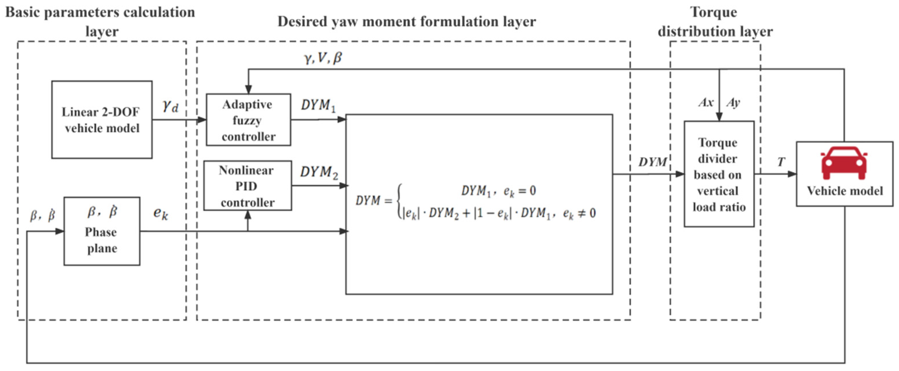
It is expected that the yaw moment formulation layer includes a stability domain calculation module, an instability compensation module, and a phase plane judgment calculation module. Yaw moment DYM1 is calculated by the fuzzy controller in the stability domain, and yaw moment DYM2 is calculated by the PID control in the instability compensation module. Finally, the phase plane judgment calculation module calculates the desired yaw moment, and the final output of DYM is based on the judgment condition of the stable parameter, e k .

4.2.1. Adaptive Fuzzy Controller

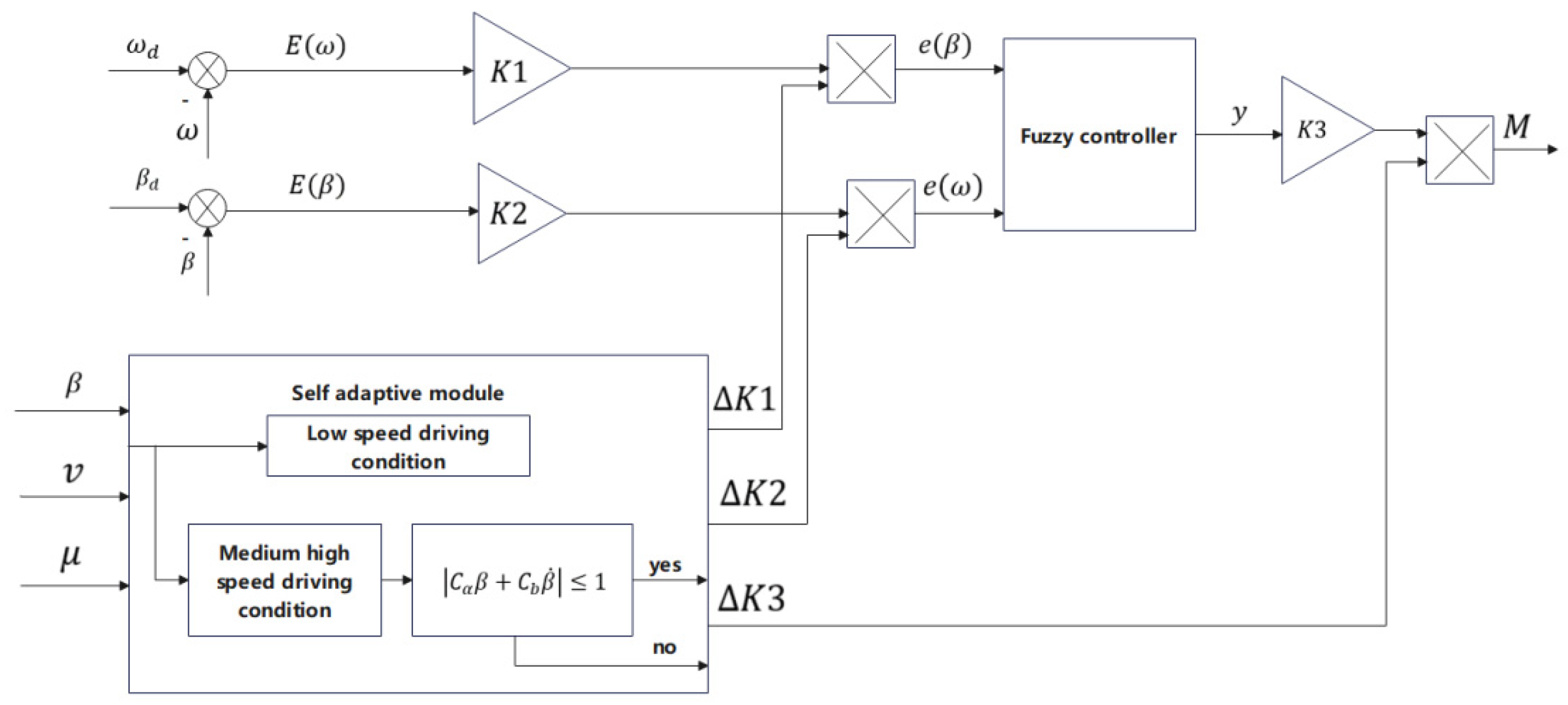
The adaptive fuzzy controller developed in this paper can dynamically adjust the quantization factor and scale factor to determine the desired yaw moment, thereby achieving the most suitable control scheme for the current operating conditions. When driving on a road with a high adhesion coefficient, the vehicle’s operating conditions are optimal. During vehicle turning, if there is a deviation between the actual and expected values of the yaw rate and sideslip angle, the quantization factor and scale factor can be simultaneously increased. This allows the actual yaw rate and sideslip angle to quickly converge to the expected values, thereby enhancing the response speed of the control system. Conversely, when driving on a road with a low adhesion coefficient, the vehicle’s operating conditions are suboptimal. In the event of a deviation between the actual and expected values of the yaw rate and sideslip angle during vehicle turning, the proportional factor output by the fuzzy controller can be reduced by increasing the quantified factor of the yaw rate and sideslip angle. This ensures an accelerated response of the control system and prevents excessive torque difference between the left and right sides of the bus, thereby enabling better performances on road surfaces with low adhesion. The design of the adaptive fuzzy controller is illustrated in Figure 5.
The adaptive fuzzy control algorithm is as follows:
e ω = K 1 × K 1 · E ω e β = K 2 × K 2 · E β  
y = f 2 e ω , e β
In Formula (13), f 2 is the functional relationship between the input and output of the adaptive fuzzy control system, which is determined by the controller parameters and the de-fuzzification mode. It can be seen from Equations (12) and (13) that the input of the fuzzy controller not only depends on the input deviations E(ω) and E(β) and the quantization factors K1 and K2, but also on ∆K1 and ∆K2 as output by the adaptive module. Similarly, the magnitude of the expected swaying moment, M, depends not only on scale factor K3 but also on ∆K3, as output by the adaptive module. The magnitude of the expected yaw moment, M, is as follows:
M = K 3 + K 3 · f 2 e ω , e β
In the process of its operation, the adaptive module can adjust the expected yaw moment, M, of the vehicle according to the corresponding values of ∆K1, ∆K2, and ∆K3, as output during actual working conditions; therefore, the vehicle can keep the best running state under any working conditions. Considering the calculation speed of the algorithm, the design of the adaptive module is as follows:
The inputs in the adaptive module are the speed, yaw rate, sideslip angle, and road adhesion coefficient, which can output the additional quantization factors ∆K1 and ∆K2, as well as scale factor ∆K3, through additional fuzzy control according to the driving conditions of the vehicle and the actual yaw rate and sideslip angle of the vehicle to ensure the control effect and response speed. When the vehicle is running at a low speed and turning, it is believed that the vehicle can meet the requirements for stable operation only by controlling the yaw rate. The adaptive module will shield the deviation value of the sideslip angle. At the same time, in order to improve the response speed of the control, the module needs to increase the control effect of the pendulum velocity deviation and the total amplification ratio of the system, that is, the outputs K 1 > 1 , K 2 = 0 ,     a n d   K 3 > 1 under this working condition. When the vehicle is driving at a high speed and turning, the change rate of the sideslip angle and the sideslip angle will be limited to C a β + C b β ˙ 1 [21]. When this range is not exceeded, the main control objective is to ensure the stability of the driving direction of the vehicle, as well as the steering speed of the vehicle. The yaw rate and sideslip angle are controlled simultaneously. At this time, the yaw rate and sideslip angle of the vehicle are equally important. The values of the two quantization factors output by the adaptive module are equal, that is, K 1 = K 2 > 1 . At the same time, when the vehicle is running at medium and high speeds, in order to ensure the stability while driving, the torque difference on both sides should be reduced, that is, the output K 3 < 1 . When this range is exceeded, the only control objective is to ensure the stability of the driving direction of the vehicle. At this time, it is believed that control of the yaw rate will no longer play a role in vehicle stability, so only the control of the sideslip angle is used to ensure the vehicle operates stably. The adaptive module will shield the difference in the yaw rate. That is, the outputs are K 1 = 0 , K 2 > 1 ,   a n d   K 3 < 1 . Through an analysis of the vehicle dynamics stability, and with reference to a large number of documents, C a = 4.386 and C b = 2.562 [
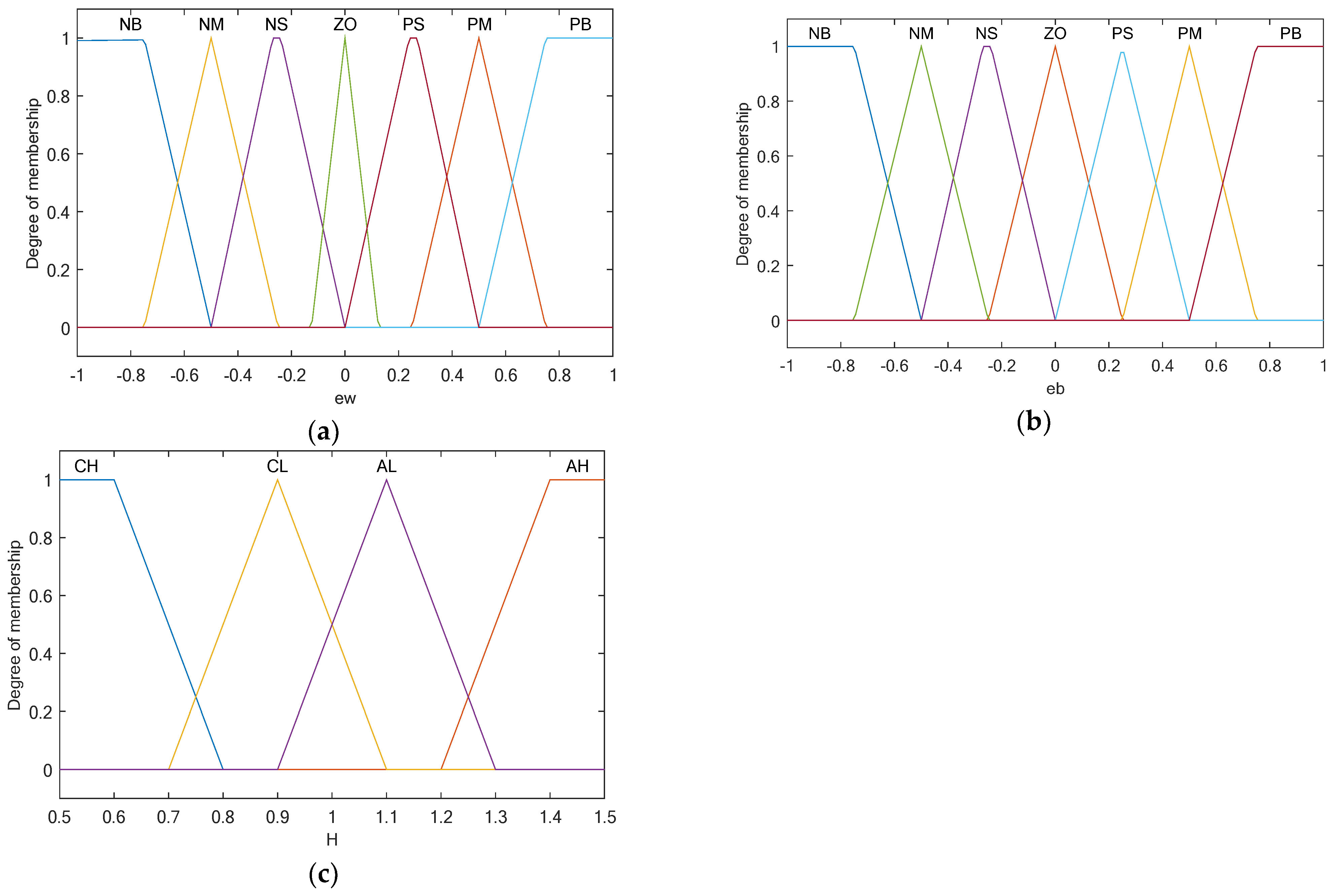
22]. The fuzzy control inputs of the adaptive module are the deviations from the ideal values of the yaw rate and the sideslip angle by the actual values, and the outputs are the additional quantization factors and scale factor of the outer fuzzy controller. There are seven fuzzy sets for the deviation between the input yaw rate and the sideslip angle of the center of mass, which are, respectively, negative large (NB), negative medium (NM), negative small (NS), zero (ZO), positive small (PS), positive medium (PM), and positive large (PB). There are four fuzzy sets for the additional quantization factor and scale factor outputs. Figure 6a–c show the corresponding membership function.
The fuzzy rules for the adjustment of the quantization factors and scale factor are shown in Table 5:
The outer fuzzy controller designed in this paper used fuzzy exact values of the deviation of the yaw rate and sideslip angle, E ( ω ) and E ( β ) , into seven fuzzy sets, which were negative large (NB), negative medium (NM), negative small (NS), zero (ZO), positive small (PS), positive medium (PM), and positive large (PB). The output variable M is divided into nine fuzzy sets, which are negative very large (NVB), negative large (NB), negative medium (NM), negative small (NS), zero (ZO), positive small (PS), positive medium (PM), positive large (PB), and positive very large (PVB). Figure 7a–c below show the corresponding membership function.
Fuzzy reasoning is the core of fuzzy control; that is, the combination of input variables and output variables of the fuzzy controller forms a one-to-one corresponding relationship rule, according to experts. The reasoning relationships, with 49 fuzzy rules, used in this paper are shown in Table 6.
Also, the weighted average method was chosen to conduct the de-fuzzification. Finally, the calculation formula of the desired yaw moment, M, is shown in Equation (15).
M = ( K 3 + Δ K 3 ) × i = 0 m y c i μ A ω i [ ( K 1 + Δ K 1 ) × E ( ω ) ] μ A β [ ( K 2 + Δ K 2 ) × E ( β ) ] i = 0 m μ A ω i [ ( K 1 + Δ K 1 ) × E ( ω ) ] μ A β [ ( K 2 + Δ K 2 ) × E ( β ) ]

4.2.2. Nonlinear PID Controller

A traditional PID control is a linear combination of errors, which can achieve a good control effect on linear and near-linear systems. Its general form is as follows:
u t = K p e t + K i 0 t e τ d τ + K d d e t d t
where K p is the proportional gain; K i is the integral gain; K d is the differential gain; and e t is the deviation.
The vehicle dynamics model is a nonlinear model, and this linear combination is not the best combination mode in the nonlinear model. The more suitable and effective combination form is in the range of a nonlinear combination. Therefore, a nonlinear combination based on nonlinear PID control is proposed in this paper, as shown in the following equation:
u = k p f a l e 1 , α 1 , L + k d f a l e 2 , α 2 , L
where 0 < α 1 < 1 < α 2 ; e 1 is the difference between the output of the current controlled object and the set value of the controlled object; e 2 is the difference between the output of the current controlled object and the change rate of the set value of the controlled object; and L is the interval length of the linear segment. The f a l function is a saturation function, as shown in Equation (18), as follows:
f a l e , α , δ = e L α 1                                 , e L e α s g n e                 , e > L
In this paper, the stability parameter, e k , was controlled, and the additional desired torque was output.

4.3. Torque Distribution Layer

In the four-wheel torque distribution layer, the vertical load transfer of a vehicle under longitudinal and lateral accelerations is estimated. Based on the desired yaw moment DYM constraint, the four-wheel torques, T f l ,   T f l r ,   T r l , and   T r r are calculated.
During the steering process, the lateral movement of the vehicle will lead to the transfer of the vertical load of the four wheels. Under the actions of the longitudinal acceleration and lateral acceleration, the vertical axle load of a four-wheel vehicle can be approximated by the following formula [23]:
F z f l = M · g · b 2 a + b M · a x · h 2 a + b M · a y · h a d a + b F z f r = M · g · b 2 a + b M · a x · h 2 a + b + M · a y · h a d a + b F z r l = M · g · b 2 a + b + M · a x · h 2 a + b M · a y · h b d a + b F z r r = M · g · b 2 a + b + M · a x · h 2 a + b + M · a y · h b d a + b
where a is the distance between the front axle and the center of mass of the car; b is the distance between the rear axle and the car’s center of mass; h is the distance between the car’s center of mass and the ground; and d is the mean wheel pitch.
Based on the estimated four-wheel vertical load, the four-wheel torque distribution relationship is as follows:
T f l + T f r · c o s δ + T r l + T r r = F x · r T f r T f l c o s δ + T r r T r l r · d 2 + T f l + T f r r · a s i n δ = D Y M K = F z f l + F z f r F z r l + F z r r T f l = K T r l T f r = K T r r

5. Simulation and Verification of the Electronic Differential Control Strategy Based on the Phase Plane

5.1. J-Turn Working Conditions Simulation Experiment

The steering wheel input was set to peak at 235° within 0.2 s and it was maintained for 4.67 s at the peak. The input of the steering wheel angle is shown in Figure 8a. The vehicle had an initial speed of 60 km/h and maintained that speed. The road adhesion coefficient was 0.85.
The simulation results are shown in the Figure 8 and Table 7. The electronic differential control strategy developed in this paper demonstrated a peak stability parameter, e k , of 0.550, while the torque average distribution strategy exhibited a peak stability parameter, | e k | , of 0.580, representing a 5.2% increase over the average torque distribution strategy. Under these operating conditions, the average stability parameter, | e k | , of the designed control strategy was 0.060, compared to 0.066 for the torque average distribution strategy, marking a 9.1% increase. These results indicate that the electronic differential control strategy designed in this paper can significantly extend the length of time a vehicle is in the stability region and reduce the tendency toward instability.
Moreover, the strategy’s peak value of | β | in this paper was 0.096, with the peak value of | β | for the torque average distribution strategy being 0.108, reflecting an 11.1% increase. The strategy’s average value of | β | was 0.018, compared to 0.019 for the torque average distribution strategy, resulting in a 5.3% improvement.
Additionally, the average difference between the actual and desired yaw rates with this study’s strategy was 0.073 rad/s, while the average according to the torque average distribution strategy was 0.075 rad/s, demonstrating a 2.7% enhancement. These findings suggest that the electronic differential control strategy designed in this paper can better track a driver’s desired trajectory and improve control stability.

5.2. Sinusoidal Stagnation Conditions Simulation Experiment

The steering wheel angle input was set to carry out a single cycle of sinusoidal input at a frequency of 0.7 Hz, with an amplitude of 150°, a pause of 500 ms at the second wave peak, and then a return to positive, as shown in Figure 9a. The vehicle had an initial speed of 80 km/h and maintained that speed. The road adhesion coefficient was set as 0.85.
The simulation results are shown in the Figure 9 and Table 8. The electronic differential control strategy developed in this paper demonstrated a peak stability parameter, e k , of 0.657, while the torque average distribution strategy exhibited a peak stability parameter, e k , of 0.794, representing a 17.3% increase over the average torque distribution strategy. Under these operating conditions, the average stability parameter, e k , of the designed control strategy was 0.094, compared to 0.313 for the torque average distribution strategy, marking a 70.0% increase. These results indicate that the electronic differential control strategy designed in this paper can significantly extend the length of time a vehicle is in the stability region and reduce the tendency toward instability.
Moreover, the strategy’s peak value of | β | in this paper was 0.152, with the peak value of | β | for the torque average distribution strategy being 0.384, reflecting a 60.5% increase. The strategy’s average value of | β | was 0.024, compared to 0.118 for the torque average distribution strategy, resulting in a 79.7% improvement.
Additionally, the average difference between the actual and the desired yaw rates with this study’s strategy was 0.084 rad/s, while the average with the torque average distribution strategy was 0.271 rad/s, demonstrating a 69.0% enhancement. These findings suggest that the electronic differential control strategy designed in this paper can better track the driver’s desired trajectory and improve the control stability.

5.3. Serpentine Conditions Simulation Experiment

The vehicle’s initial speed was set to 100 km/h, and this speed was maintained. The vehicle followed the route shown in Figure 10, where L is 30 m. The road adhesion coefficient was set to 0.85.
The simulation results are shown in the Figure 11 and Table 9. The peak value of | β | for the strategy in this paper was 0.042, with the peak value of | β | with the torque average distribution strategy being 0.046, reflecting an 8.4% increase. The average value of | β | for the strategy was 0.021, compared to 0.023 for the torque average distribution strategy, resulting in an 8.1% improvement.
The average difference between the actual and the desired yaw rates with the research strategy was 0.055 rad/s, while the average with the torque average distribution strategy was 0.063 rad/s, demonstrating a 12.9% enhancement. These findings suggest that the electronic differential control strategy designed in this paper can better track the driver’s desired trajectory and improve the control stability.

5.4. Double-Lane Change Conditions Simulation Experiment

The vehicle’s initial speed was set to 100 km/h, and this speed was maintained. The road adhesion coefficient was 0.85, and a double shift runway, as shown in Figure 12, was used.
The simulation results are shown in the Figure 13 and Table 10. The electronic differential control strategy developed in this paper demonstrated a peak stability parameter, | e k | , of 0.557, while the torque average distribution strategy exhibited a peak stability parameter, e k , of 0.657, representing a 1.8% increase over the average torque distribution strategy. Under these operating conditions, the average stability parameter, | e k | , of the designed control strategy was 0.093, compared to 0.099 for the torque average distribution strategy, marking a 5.5% increase. These results indicate that the electronic differential control strategy designed in this paper can significantly extend the length of time a vehicle is in the stability region and reduce the tendency toward instability.
Moreover, the strategy’s peak value of | β | in this paper was 0.217, with the peak value of | β | for the torque average distribution strategy being 0.219, reflecting an 1.1% increase. The strategy’s average value of | β | was 0.039, compared to 0.041 for the torque average distribution strategy, resulting in a 4.2% improvement.
Additionally, the average difference between the actual and the desired yaw rates with this study’s strategy was 0.164 rad/s, while the average with the torque average distribution strategy was 0.175 rad/s, demonstrating a 6.39% enhancement. These findings suggest that the electronic differential control strategy designed in this paper can better track a driver’s desired trajectory and improve the control stability.

6. Conclusions

This study focused on distributed drive electric vehicles and aimed to design an electronic differential control strategy based on the phase plane method. To achieve this, a MATLAB/Simulink and CarSim cosimulation platform was built. The control effect of the electronic differential control strategy was compared to that of the average distribution strategy. The simulation results demonstrate that the proposed strategy enhances a vehicle’s handling and stability performances.
The division of the stability region of the phase plane needs to be estimated by the double-line method or other methods. The accuracy of the estimation also affects the accuracy of the control strategy. In follow-up research, the authors will continue to explore improving the phase plane accuracy.

Author Contributions

Conceptualization, S.Z. and C.K.; Methodology, S.Z., C.K., H.C. and J.G.; Software, Y.X.; Validation, Y.X.; Formal analysis, Y.X. and J.G.; Investigation, Y.X.; Writing—original draft, Y.X.; Writing—review and editing, S.Z. and H.C.; Supervision, L.L. and Y.R.; Project administration, S.Z. All authors have read and agreed to the published version of the manuscript.

Funding

We gratefully acknowledge the financial support for this research by the following project: Control design of new energy vehicle air conditioning compressor based on intelligent multi-objective optimization (ZDLQ2020002).

Institutional Review Board Statement

Not applicable.

Informed Consent Statement

Not applicable.

Data Availability Statement

The original contributions presented in the study are included in the article, further inquiries can be directed to the corresponding author.

Conflicts of Interest

The authors declare no conflicts of interest.

References

  1. Yu, Z.P.; Feng, Y.; Xiong, L. Review on Vehicle Dynamics Control of Distributed Drive Electric Vehicle. J. Mech. Eng. 2013, 49, 105–114. [Google Scholar] [CrossRef]
  2. Zhang, D.; Liu, G.H.; Zhao, W.X. Overview of Multimotor Independent Drive of Electric Vehicles. Automob. Technol. 2015, 10, 1–6. [Google Scholar]
  3. Ma, H.J. Research on Electronic Differential Control System of Electric Vehicle. Master’s Thesis, Zhejiang University, Hangzhou, China, 2016. [Google Scholar]
  4. Wu, N. Motion Simulation Research on Four-wheel Steering System of Electric Vehicle. Master’s Thesis, South China University of Technology, Guangzhou, China, 2015. [Google Scholar]
  5. Peng, S.L. Research on Differential Control Strategy of Electric Wheel Vehicle. Master’s Thesis, Wuhan University of Science and Technology, Wuhan, China, 2011. [Google Scholar]
  6. Feng, J.D. Wheel Motor Drive Electric Vehicle Stability Control Limit Condition. Master’s Thesis, Dalian University of Technology, Dalian, China, 2020. [Google Scholar]
  7. Lu, C.Z. Research on Vehicle Stability Control Algorithm Based on State Variable Constraints. Master’s Thesis, Jiangsu University, Zhenjiang, China, 2019. [Google Scholar]
  8. Lee, J.S.; Ryoo, Y.J.; Lim, Y.C.; Freere, P.; Kim, T.G.; Son, S.J.; Kim, E.S. A neural network model of electric differential system for electric vehicle. In Proceedings of the 2000 26th Annual Conference of the IEEE Industrial Electronics Society. IECON 2000. 2000 IEEE International Conference on Industrial Electronics, Control and Instrumentation. 21st Century Technologies, Nagoya, Japan, 22–28 October 2000. [Google Scholar]
  9. Yang, Y.; Xing, X. Design of electric differential system for an electric vehicle with dual wheel motors. In Proceedings of the 2008 47th IEEE Conference on Decision and Control, Cancun, Mexico, 9–11 December 2008. [Google Scholar]
  10. Tabbache, B.; Kheloui, A.; Benbouzid, M.E.H. An Adaptive Electric Differential for Electric Vehicles Motion Stabilization. IEEE Trans. Veh. Technol. 2011, 60, 104–110. [Google Scholar] [CrossRef]
  11. Zhai, L.; Sun, T.; Wang, J. Electronic stability control based on motor driving and braking torque distribution for a four in-wheel motor drive electric vehicle. IEEE Trans. Veh. Technol. 2016, 65, 4726–4739. [Google Scholar] [CrossRef]
  12. Liu, J.; Chen, P.; Li, D.F. Vehicle Stability Control based on Phase Plane Method. Chin. J. Eng. Des. 2016, 23, 409–416. [Google Scholar]
  13. Han, Z.; Xu, N.; Chen, H.; Huang, Y.; Zhao, B. Energy-efficient control of electric vehicles based on linear quadratic regulator and phase plane analysis. Appl. Energy 2018, 213, 639–657. [Google Scholar] [CrossRef]
  14. Di Cairano, S.; Tseng, H.E.; Bernardini, D.; Bemporad, A. Vehicle yaw stability control by coordinated active front steering and differential braking in the tire sideslip angles domain. IEEE Trans. Control Syst. Technol. 2013, 21, 1236–1248. [Google Scholar] [CrossRef]
  15. Zhong, L.F.; Peng, Y.H.; Jiang, M. Distributed drive electric vehicle stability control based on phase plane. J. Automob. Eng. Lancet 2021, 43, 721–729+738. [Google Scholar]
  16. Beal, C.; Bobier, C.G.; Gerdes, J.C. Controlling vehicle instability through stable handling envelopes. In Proceedings of the ASME 2011 Dynamic Systems and Control Conference and Bath/ASME Symposium on Fluid Power and Motion Control, Arlington, Virginia, USA, 31 October–2 November 2011; American Society of Mechanical Engineers: New Youk, NY, USA, 2011. [Google Scholar]
  17. Beal, C.; Christian, G. Model predictive control for vehicle stabilization at the limits of handling. IEEE Trans. Control Syst. Technol. 2012, 21, 1258–1269. [Google Scholar] [CrossRef]
  18. Huang, K.; Wen, S.C. Based on the phase plane of the electric car operation stability model predictive control. J. Automot. Technol. 2023, 12, 47–53. [Google Scholar]
  19. Hu, Y.Z. Stability Control Research of Four-Wheel Independent Drive Electric Vehicle with Driver in the Loop. Master’s Thesis, Hefei University of Technology, Hefei, China, 2017. [Google Scholar]
  20. Li, H.J. Research on Vehicle Handling and Stability Control Based on Phase Plane Analysis. Master’s Thesis, Hefei University of Technology, Hefei, China, 2018. [Google Scholar]
  21. Zhang, C.C. Simulation Study of ESP Automotive Electronic Stability System. Master’s Thesis, Shandong University, Jinan, China, 2007. [Google Scholar]
  22. Chen, S. Design of Distributed Drive Control System for Wheel Side Rear-Drive Electric Bus. Master’s Thesis, Hangzhou University of Electronic Science and Technology, Hangzhou, China, 2023. [Google Scholar]
  23. Fu, H. Research on the Estimation and Control Strategy of the Lateral Deflection Angle of the Center of Mass of an Automotive Electronic Stability System. Ph.D. Thesis, Jilin University, Changchun, China, 2008. [Google Scholar]
Figure 1. Vehicle dynamics model.
Wevj 15 00243 g001
Figure 2. Phase plane Simulink simulation model.
Wevj 15 00243 g002
Figure 3. Schematic diagram of the phase plane stability region boundary.
Wevj 15 00243 g003
Figure 4. Structure diagram of the electronic differential control strategy based on the phase plane.
Wevj 15 00243 g004
Figure 5. Adaptive fuzzy controller.
Wevj 15 00243 g005
Figure 6. Membership function of the fuzzy controller in the adaptive module: (a) yaw rate deviation membership function; (b) sideslip angle deviation membership function; (c) deviation in the additional scale factor and quantification factors membership function.
Wevj 15 00243 g006
Figure 7. Membership function of the outer fuzzy controller: (a) yaw rate deviation membership function; (b) sideslip angle deviation membership function; (c) desired yaw moment membership function.
Wevj 15 00243 g007
Figure 8. J-turn working conditions test diagram.
Wevj 15 00243 g008
Figure 9. Sinusoidal stagnation conditions test diagram.
Wevj 15 00243 g009aWevj 15 00243 g009b
Figure 10. Car track diagram.
Wevj 15 00243 g010
Figure 11. Serpentine conditions test diagrams.
Wevj 15 00243 g011
Figure 12. Car track diagram.
Wevj 15 00243 g012
Figure 13. Serpentine conditions test diagram.
Wevj 15 00243 g013
Table 1. Vehicle parameters.
ParameterValue
Curb weight/Kg1620
Overall dimensions/mm3775 × 1665 × 1690
Moment of inertia/kg-m22032.1
Wheelbase/mm2450
Distance from front axle to center of mass/mm1050
Distance from rear axle to centroid/mm1400
Centroid height/mm500
Front track width/mm1430
Rear track width/mm1430
Axle load distribution/Kg915/710
Tire specifications175/70 R13
Table 2. Boundary coefficient of the stability region of the phase plane of the sideslip angle under different speed conditions.
Speed (m/s)AB
5.033.803.80
7.523.501.78
10.011.601.00
12.510.650.84
15.09.650.60
17.58.480.60
20.07.900.60
22.57.340.55
25.06.600.55
27.56.350.55
30.05.800.55
32.55.100.55
35.04.300.55
Table 3. Boundary coefficient of the stability region of the phase plane of the sideslip angle under different speed conditions.
Coefficient of AdhesionAB
0.11.200.10
0.22.000.20
0.33.300.30
0.44.000.35
0.55.300.52
0.66.100.54
0.76.700.56
0.87.900.58
0.98.500.60
1.010.700.61
Table 4. Boundary coefficient of the stability region of the phase plane of the sideslip angle under different speed conditions.
Front Wheel Angle B
0.50.04
1.00.07
1.50.11
2.00.14
2.50.18
3.00.24
3.50.32
4.00.39
Table 5. Fuzzy rules for the adjustments of the quantization factors and scale factor.
e ω \ e β NBNMNSZOPSPMPB
NBCHCHCLALCLCHCH
NMCHCHALAHALCHCH
NSCHCLALAHALCLCH
ZOCHCLALAHALCLCH
PSCHCLALAHALCLCH
PMCHCLALAHALCHCH
PBCHCHCLALCLCHCH
Table 6. Fuzzy control fuzzy rule table.
e ω \ e β NBNMNSZOPSPMPB
NBNVBNVBNVBNBNBNMNB
NMNBNBNBNMNMNSNS
NSNBNMNMNMNSZOZO
ZONMNMNSZOZOPSPS
PSNMNSZOPSPSPMPM
PMNSZOPSPMPMPBPB
PBZOPSPMPBPBPVBPVB
Table 7. Simulation experiment’s data under the J-turn working conditions.
Equal Distribution MethodPhase Plane MethodEffect of Optimization
Peak of e k 0.5800.5505.2%
Mean of e k 0.0660.0609.1%
Peak of β 0.108 rad0.096 rad11.1%
Mean of β 0.019 rad0.018 rad5.3%
Mean of ω 0.075 rad/s0.073 rad/s2.7%
Table 8. Simulation experiment’s data under the sinusoidal stagnation condition.
Equal Distribution MethodPhase Plane MethodEffect of Optimization
Peak   of   e k 0.7940.65717.3%
Mean   of   e k 0.3130.09470.0%
Peak   of   β 0.384 rad0.152 rad60.5%
Mean   of   β 0.118 rad0.024 rad79.7%
Mean   of   ω 0.271 rad/s0.084 rad/s69.0%
Table 9. Simulation experiment’s data under a serpentine condition.
Equal Distribution MethodPhase Plane MethodEffect of Optimization
Peak of β 0.042 rad0.046 rad8.4%
Mean of β 0.021 rad0.023 rad8.1%
Mean of ω 0.055 rad/s0.063 rad/s12.9%
Table 10. Simulation experiment’s data under the double-lane change conditions.
Equal Distribution MethodPhase Plane MethodEffect of Optimization
Peak   of   e k 0.5570.5671.8%
Mean   of   e k 0.0930.0995.5%
Peak   of   β 0.217 rad0.219 rad1.1%
Mean   of   β 0.039 rad0.041 rad4.2%
Mean   of   ω 0.164 rad/s0.175 rad/s6.39%
Disclaimer/Publisher’s Note: The statements, opinions and data contained in all publications are solely those of the individual author(s) and contributor(s) and not of MDPI and/or the editor(s). MDPI and/or the editor(s) disclaim responsibility for any injury to people or property resulting from any ideas, methods, instructions or products referred to in the content.

