Path-Following Control of Unmanned Vehicles Based on Optimal Preview Time Model Predictive Control

Abstract

In order to reduce the lateral error of path-following control of unmanned vehicles under variable curvature paths, we propose a path-following control strategy for unmanned vehicles based on optimal preview time model predictive control (OP-MPC). The strategy includes the longitudinal speed limit, the optimal preview time surface, and the model predictive control (MPC)controller. The longitudinal speed limit controls speed to prevent vehicle rollover and sideslip. The optimal preview time surface adjusts the preview time according to the vehicle speed and path curvature. The preview point determined by the preview time is used as the reference waypoint of OP-MPC controller. Finally, the effectiveness of the strategy was verified through simulation and with the real unmanned vehicle. The maximum lateral deviation obtained by the OP-MPC controller was reduced from 0.522 m to 0.145 m under the simulation compared with an MPC controller. The maximum lateral deviation obtained by the OP-MPC controller was reduced from 0.5185 m to 0.2298 m under the real unmanned vehicle compared with the MPC controller.

1. Introduction

Unmanned driving not only reduces the incidence of traffic accidents caused by operational errors but also improves traffic efficiency [1]. Therefore, unmanned driving technology has become a popular research topic in the field of automatic control [2]. Path-following control is a key technology for unmanned driving research [3]. It mainly controls the turning angle of the steering wheel of the vehicle to make the vehicles trace the desired path and reach the target position [4]. Path-following control algorithms include robust control, synovial control, model predictive control (MPC), and so on.

MPC has the advantages of handling state variables, controlling input constraints, achieving driver comfort, time consumption, and tracking accuracy [5]. It is an effective and feasible path-tracking control method [6]. Sun C. proposed a MPC path-following controller with switched tracking error, which can reduce lateral tracking deviation and maintain vehicle stability under normal and high-speed conditions [7]. A nonlinear model predictive control (NMPC) based on a simplified third-order vehicle model was proposed to track a given path by controlling the steering of the front wheels while satisfying various physical and design constraints [8]. Falcone [9] developed a linear time-varying model predictive control (LTV-MPC) method, combined with braking force distribution to achieve vehicle motion stability control, with good real-time performance. Bai et al. [10] designed a novel controller based on NMPC to improve the path-tracking performance of unmanned vehicles, but this method can only work at different longitudinal speeds and cannot automatically adjust the longitudinal speed. Xu et al. [11] designed a path-following control algorithm for preview steering and described the path-following problem as an optimal control problem with dynamic disturbances, i.e., the future road curvature, which can improve the path-following accuracy, but this method path-following is not considered under variable curvature condition. Sun et al. [12] proposed a path-tracking controller based on LTV-MPC, and they improved the control accuracy by adjusting the speed. Guo et al. [13] proposed a dual-envelope LTV-MPC path-following controller, which considered the front-wheel turning angle constraint and the front-wheel turning angular velocity constraint, and considered the case when the ground adhesion coefficient was low. Aiming at the uncertainty of model parameters and the influence of external disturbance, Ji et al. [14] proposed a robust path-following control method based on an adaptive neural network. Yang et al. [15] proposed an LTV-MPC method combining active steering control and a direct yaw control strategy to improve path-following accuracy and vehicle driving stability when the ground adhesion coefficient is low. Bai et al. [16] proposed an MPC control framework that can actively adjust the longitudinal speed according to the path information during path tracking and has good following accuracy. Yuet al. [17] designed a path-following controller considering vehicle dynamics, actuators, and state constraints based on the MPC method. The authors of [18] propose a fuzzy adaptive predictive time control strategy that takes pavement curvature and lateral acceleration as the system inputs and fixed prediction time as the system output. It is very difficult to make fuzzy rules and rationalize them manually. The authors of [19] proposed an adaptive preview tracking control method considering road curvature and vehicle speed, designed the preview time according to different vehicle parameters and road conditions, improved the adaptability to road conditions and speed information, and further optimized the path-tracking accuracy.

The existing MPC following methods for unmanned vehicles do not consider the influence of vehicle speed and path curvature on the path-following accuracy of unmanned vehicles, and the tracking performance and stability of unmanned vehicles on paths with variable curvature are reduced; they cannot even track paths.

Therefore, in view of the low accuracy and stability of intelligent vehicle-tracking control under variable curvature paths, a new MPC strategy is proposed to ensure the path-tracking accuracy and the stability and safety of unmanned vehicles. The main contributions of this paper are as follows:

(1)

An unmanned vehicle path-following control strategy based on optimal preview time MPC(OP-MPC) for unmanned vehicles is proposed, which includes the longitudinal speed limit, the optimal preview time surface, and the MPC controller.

(2)

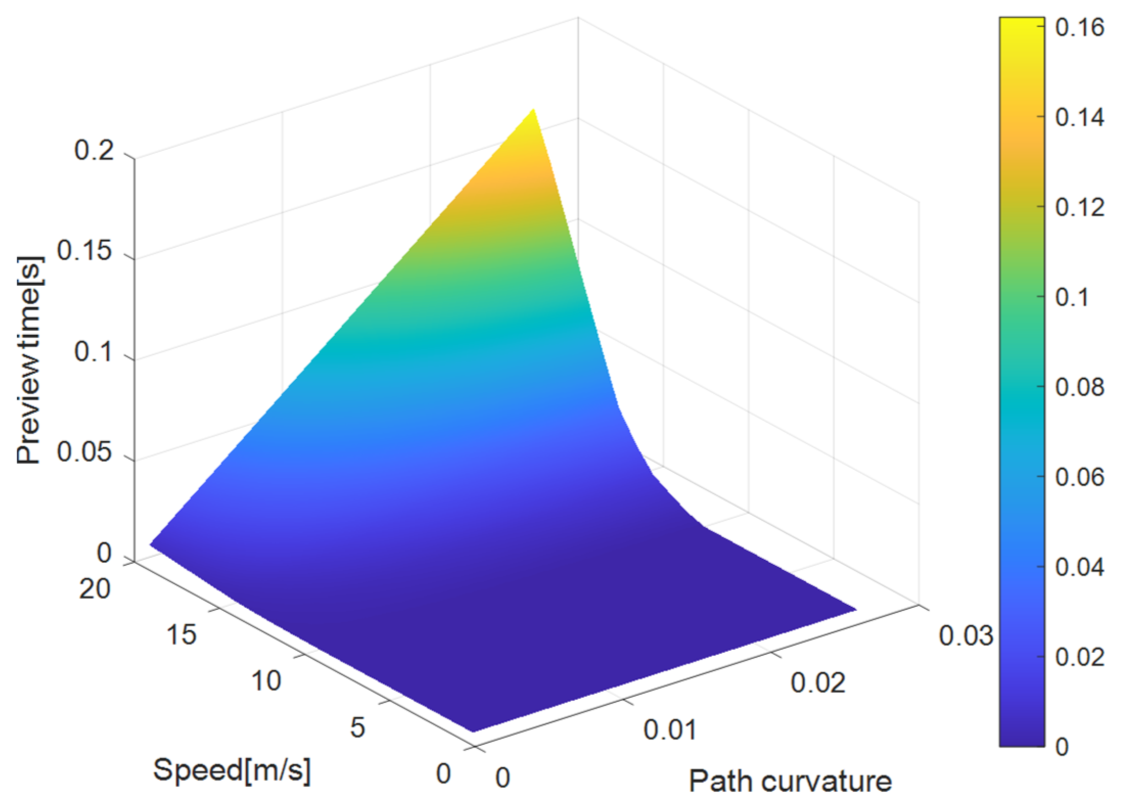
The particle swarm optimization (PSO) algorithm was used to obtain the optimal preview time under different vehicle speeds, and road curvatures. The linear interpolation was used to obtain the optimal preview time surface.

(3)

The longitudinal speed limit controls speed to prevent vehicle rollover and sideslip.

The performance of the path-following control strategy was verified on the Carsim-Simulink platform, and the effectiveness of the strategy was tested with a real unmanned vehicle.

The structure of this paper is organized as follows: Section 1 designs the presents of the longitudinal speed controller; Section 2 introduces the vehicle dynamics model and the MPC problem formulation; Section 3 obtains the optimal preview time surface; Section 4 introduces the control simulation and real vehicle testing of the algorithm; Section 5 concludes the paper.

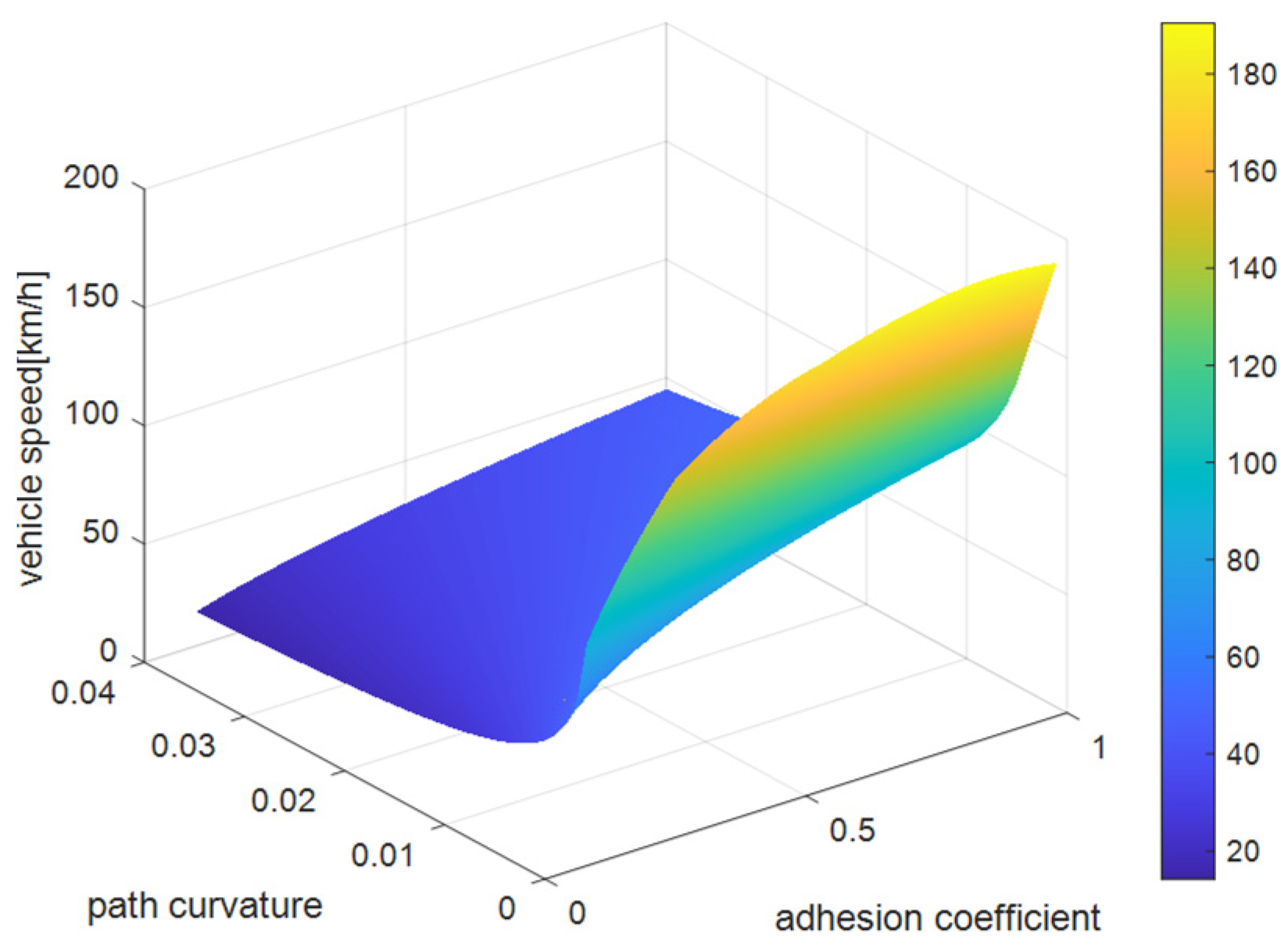
2. Longitudinal Speed Limit

The steering operation of the vehicle on roads with variable curvature is the main cause of side-slip and roll-over. Therefore, preventing vehicle side slip and roll-over during the turning process is the key to the stable driving of the vehicle. Controlling the longitudinal speed of the vehicle in the variable-curvature path can effectively protect the vehicle from side slip and roll-over. The maximum speed of the vehicle is limited by the anti-sideslip and anti-rollover mechanisms:

$$u_{\lim \mathrm{it}}=\min (u_{\mathrm{safe}},u_{\max })$$

(1)

where $u_{\max }$ indicates the maximum speed of straight driving, which $u_{\mathrm{safe}}$ is a safe speed to prevent sideslip and rollover.

Table 1. Vehicle parameters.

Symbol	Parameter	Value
$L$	Wheelbase	2.910 [m]
$m$	Mass	1412 [kg]
$C_{fr},C_{fl}$	Front wheel cornering stiffness	148,970 $[N/\mathrm{rad}]$
$C_{fr},C_{rl}$	Rear wheel cornering stiffness	82,204 $[N/\mathrm{rad}]$
$a$	Distance from front wheel to center of mass	1.015 [m]
$b$	Distance from rear wheel to center of mass	1.895 [m]
$I_z$	Moment of inertia	1536.7 $[\mathrm{kg}·{\mathrm{m}}^2]$
$B$	Vehicle track	1.89 [m]

shows the parameters of the tested vehicle.

2.1. Sideslip Constraint

When the vehicle is driving on a bend, if the lateral adhesion of the wheels is less than the lateral frictional resistance between the road surface and the tires, sideslip will occur. The sideslip constraint can be simplified to

$$m|a_{\mathrm{y}}| \le m\mu g\cos \beta$$

(2)

where $\mu$ is the coefficient of friction and $\beta$ indicates the road gradient.

When the vehicle is turning in a steady state, the approximate relationship between the lateral acceleration $a_y$ and the steady-state turning radius $R_s$ is as follows:

$$|a_y| \approx v_x^2/R_s$$

(3)

where $a_y$ indicates the lateral acceleration, $R_s$ indicates the steady-state turning radius, and $v_x$ indicates the longitudinal velocity.

The steady-state turning $R_s$ of the vehicle can be obtained from the curvature of the road:

$$R_s=1/k_{\_road}$$

(4)

where $k\_road$ is the path curvature.

Based on Equations (2)–(4), the speed safety limit of anti-skid vehicles can be expressed as follows:

$$u_{\mathrm{slip}}\le k_{\mathrm{slip}}\sqrt{\mu g\cos \alpha /k_{\_road}}$$

(5)

where $k_{slip}$ is the anti-skid safety factor less than 1.

2.2. Rollover Constraint

The lateral load transfer of the vehicle is one of the main factors of the vehicle rollover. When the vehicle is driving on the road (including the lateral slope), the lateral acceleration of the vehicle exceeds a certain limit. The vertical reaction force of the inner wheel of the vehicle is zero, which causes a rollover.

$${\mathrm{F}}_i=mg(f\cos \beta +\sin \beta )$$

(6)

where $f$ is the wheel rolling resistance coefficient and $\beta$ is the road gradient.

Assuming that the road gradient $\beta$ is small.

$$\sin \beta \approx \beta ,\cos \beta \approx 1$$

(7)

Lateral acceleration causes load transfer between the inside and outside of the vehicle, causing the vehicle to roll over. In sum, the rollover constraint can be expressed as follows, Equation (8):

$$\mu (0.5mg-m|a_y|h/B)\ge F_i$$

(8)

where $h$ is the height of the center of mass of the vehicle, $\mu$ is the coefficient of friction, and $B$ is the distance between the wheels of the vehicle.

Combining Equations (6)–(8), the anti-rollover constraint can be expressed as follows:

$$u_{\mathrm{over}}\le k_{\mathrm{over}}\sqrt{(0.5mg-F_i/\mu )BR/(mh)}$$

(9)

where $k_{over}$ is the rollover safety factor less than 1.

The safe speed limit for a vehicle can be described as follows:

$$u_{\mathrm{safe}}=\min (u_{\mathrm{slip}},u_{\mathrm{over}})$$

(10)

Figure 1 shows longitudinal speed limits for different curvatures and road adhesion coefficients, which are used for the safety speed limits of driverless vehicles. The speed of the driverless vehicle can be limited to a safe range to avoid rollovers and sideslips in different path conditions.

3. Path-Following Control Based on Model Predictive Control (MPC)

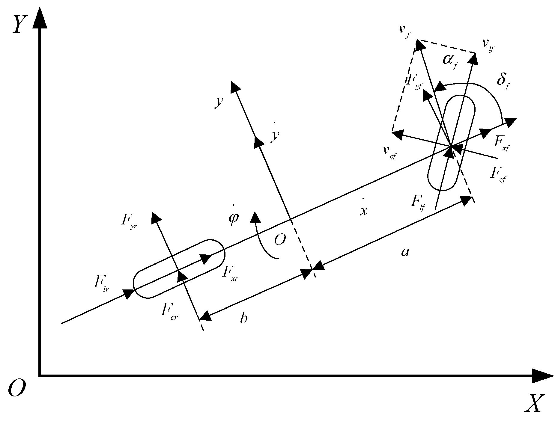
3.1. Vehicle Model

Figure 2 shows the 3-DOF nonlinear vehicle model adopted by the MPC controller.

The dynamic equations of the vehicle model, according to Newton’s second law, are as follows:

$$m\stackrel{..}{x}=m\stackrel{.}{y}\stackrel{.}{\phi }+2F_{xf}+2F_{xr}$$

(11)

$$m\stackrel{.}{y}=-m\stackrel{.}{x}\stackrel{.}{\phi }+2F_{xf}+2F_{xr}$$

(12)

$$I_z\stackrel{..}{\phi }=2a{F}_{yf}-2b{F}_{yr}$$

(13)

$$\stackrel{.}{Y}=\stackrel{.}{x}\sin (\phi )+\stackrel{.}{y}\cos (\phi )$$

(14)

$$\stackrel{.}{X}=\stackrel{.}{x}\cos (\phi )-\stackrel{.}{y}\sin (\phi )$$

(15)

where $X$, $Y$, and $\phi$ are the lateral position, longitudinal position, and heading angle of the vehicle, respectively, $F_{lf}$ and $F_{lr}$ are the longitudinal force on the front and rear tires, respectively, $F_{cf}$ and $F_{cr}$ are the lateral forces on the front and rear wheels, respectively, $F_{xf}$ and $F_{xr}$ are the resultant forces of the longitudinal tire forces acting on the front and rear axles of the vehicle, respectively, $F_{yf}$ and $F_{yr}$ are the resultant forces of the lateral tire forces acting on the front and rear axles of the vehicle, respectively and I_z is the moment of inertia. The forces in the $x$ and $y$ directions are related to the longitudinal and lateral forces as follows:

$$F_{xf}=F_{lf}\cos ({\delta }_f)-F_{cf}\sin ({\delta }_f)$$

(16)

$$F_{xr}=F_{lr}\cos ({\delta }_r)-F_{cr}\sin ({\delta }_r)$$

(17)

$$F_{yf}=F_{lf}\cos ({\delta }_f)+F_{cf}\sin ({\delta }_f)$$

(18)

$$F_{yr}=F_{lr}\cos ({\delta }_r)+F_{cr}\sin ({\delta }_r)$$

(19)

where ${\delta }_f$ and ${\delta }_r$ are the front wheel steering angles and rear wheel steering angles respectively. If the rear wheel does not turn, then ${\delta }_r=0$, the linearized tire model has a high fitting accuracy when the tire slip angle is small, and the linearized expression of the lateral tire force can be obtained by using the small-angle assumption:

$$F_{cf}=C_{cf}({\delta }_f-(\stackrel{.}{y}+a\stackrel{.}{\phi })/\stackrel{.}{x})$$

(20)

$$F_{cr}=C_{cr}(b\stackrel{.}{\phi }-\stackrel{.}{y})/\stackrel{.}{x}$$

(21)

The longitudinal force of the tire according to Hooke’s laws is as follows:

$$F_{lf}=C_{lf}{s}_f$$

(22)

$$F_{lr}=C_{lr}{s}_r$$

(23)

where $s_f$ and $s_r$ are the slip rate of the tire.

3.2. Model Predictive Control

Model predictive control (MPC) is a commonly used path-following control method. The nonlinear model of vehicle dynamics based on the small-angle assumption and the linear tire model can be expressed as follows:

$$m\stackrel{..}{y}=-m\stackrel{.}{x}\stackrel{.}{\phi }+2[C_{cf}({\delta }_f-(\stackrel{.}{y}+a\stackrel{.}{\phi })/\stackrel{.}{x})+C_{cr}(b\stackrel{.}{\phi }-\stackrel{.}{y})/\stackrel{.}{x}$$

(24)

$$m\stackrel{..}{x}=m\stackrel{.}{y}\stackrel{.}{\phi }+2[C_{lf}{s}_f+C_{cf}({\delta }_f-(\stackrel{.}{y}+a\stackrel{.}{\phi })/\stackrel{.}{x}){\delta }_f+C_{lr}{s}_r]$$

(25)

$$I_z\stackrel{..}{\phi }=2[a{C}_{cf}({\delta }_f-(\stackrel{.}{y}+a\stackrel{.}{\phi })/\stackrel{.}{x})-b{C}_{cr}(b\stackrel{.}{\phi }-\stackrel{.}{y})/\stackrel{.}{x}]$$

(26)

$$\stackrel{.}{Y}=\stackrel{.}{x}\sin (\phi )+\stackrel{.}{y}\cos (\phi )$$

(27)

$$\stackrel{.}{X}=\stackrel{.}{x}\cos (\phi )-\stackrel{.}{y}\sin (\phi )$$

(28)

In this system, the state variable is selected as $X_s={[\stackrel{.}{y},\stackrel{.}{x},\phi ,\stackrel{.}{\phi },Y,X]}^T$ and the control variable is selected as $u={\delta }_f$. The system can be described as ${\stackrel{.}{X}}_s=f(X_s,u)$.

Using the approximate linearization method to transform ${\stackrel{.}{X}}_s=f(X_s,u)$ into a linear time-varying system, expand the system ${\stackrel{.}{X}}_s=f(X_s,u)$ at the reference point $(X_{s0},u_0)$ with Taylor series and ignore higher-order terms as follows:

$${\stackrel{.}{X}}_s=f(X_s,u)=f(X_{s0},u_0)+\partial f/\partial X_s{|}_{X_{s0},u_0} d{X}_s+\partial f/\partial u{|}_{X_{s0},u_0} du$$

(29)

The state-space expression of the system is

$$d\stackrel{.}{X}=A_{0}dX+B_{0}du$$

(30)

where $dX=X_s-X_{s0}$, $du=u-u_0$, $A_0=\partial f/\partial X_s{|}_{X_{s0,u_0}}$, $B_0=\partial f/\partial u{|}_{X_{s_{0,u_0}}}$.

Using Euler’s method to discretize the system, we get

$$X_s(k+1)=A_T{X}_s(k)+B_{T}u(k)$$

(31)

where $A_T=I+A_0{T}_s$, $B_T=B_0{T}_s$, $I$ is the identity matrix, $T_s$ is the sampling time of the system, $k$ is a single current sampling time, and $k+1$ is the next sampling time.

The discrete state Equation (31) is used to construct a new state quantity as follows:

$$X_d(k)={[X_s(k)\hspace{1em}u(k-1)]}^T$$

$$X_d(k+1)=A{X}_d(k)+B\mathrm{\Delta }u(k)$$

(32)

where $A=\left[\begin{array}{cc}{A}_T& B_T\\ 0_{m\times n}& I_m\end{array}\right]$, $B=\left[\begin{array}{c}{B}_T\\ I_m\end{array}\right]$, $m=1$, $n=6$.

In order to improve the path-tracking accuracy and driving stability of the vehicle system in the path-tracking process, the performance evaluation function is defined as follows:

$$J((X_d(t),u(t-1),\mathrm{\Delta }u(k))={\displaystyle \sum _{i=1}^{N_p}||{\tilde{X}}_d(k+i|k)-{\tilde{X}}_{ref}(k+i|k)|{{|}_Q}^2}+{\displaystyle \sum _{i=1}^{N_c}\left|\right|\mathrm{\Delta }u(k+i)\left|\right|{{|}_R}^2}$$

(33)

where $t-1$ is the last sampling time, $N_p$ is the prediction step, $N_c$ is the control step, ${\tilde{X}}_d(k+i|k)$ is the predicted value for the control output, ${\tilde{X}}_{ref}(k+i|k)$ is the reference value for the control output, $\mathrm{\Delta }u(k+i|k)$ is the control increment, and $Q$, $R$ is the weight matrix, where ${\tilde{X}}_d(k+i|k)=[X_d(k),X_d(k+1),···X_d(k{+\mathrm{N}}_p)]$, ${\tilde{X}}_{ref}=[X_{ref}(k),X_{ref}(k+1),···X_{ref}(k+N_p)]$.

$$\mathrm{\Delta }u(k+1|k)=u(k+1|k)-u(k|k)$$

(34)

At time $k$, the state $X_d(k)$ is known through continuous iteration. The future state variables can be calculated as follows:

$$X_d(k+1)=A{X}_d(k)+Bu(k)$$

(35)

$$X_d(k+2)=A{X}_d(k+1)+Bu(k+1)=A^2{X}_d(k)+ABu(k)+Bu(k+1)$$

(36)

$$X_d(k+N_p)=A^{N_p}{X}_d(k)+Bu(k+1)=A^{N_p}{X}_d(k)+A^{N_p-1}Bu(k)+{\displaystyle \sum _{i=1}^{N_p-N_c+1}{A}^{i-1}}Bu(k+N-1)$$

(37)

Equations (35)–(37) can be simplified to

$${\tilde{X}}_d(k+1)=A_m{X}_d(k)+B_m\mathrm{\Delta }U(k)$$

(38)

where $A_m=\left[\begin{array}{c}A\\ A^2\\ A^3\\ ···\\ A^{N_p}\end{array}\right]$, $B_m=\left[\begin{array}{ccccc}B& 0& 0& ···& 0\\ AB& B& 0& ···& 0\\ A^{2}B& AB& B& ···& \\ ···& ···& ···& ···& ···\\ A^{N_p-1}B& A^{N_p-2}B& A^{N_p-3}B& ···& B\end{array}\right]$

• $\mathrm{\Delta }U(k+1|k)=[\mathrm{\Delta }u(k),\mathrm{\Delta }u(k+1),···\mathrm{\Delta }u(k+N_c)]$, $\widetilde{X_d}(k+1)=[X_d(k+1),X_d(k+2),···X_d(k+N_p)]$

The performance evaluation function can be simplified as follows:

$$J={(\widetilde{X_d}-{\tilde{X}}_{ref})}^{T}Q(\widetilde{X_d}-{\tilde{X}}_{ref})+\mathrm{\Delta }{U}^{T}R\mathrm{\Delta }U$$

(39)

where $Q$, $R$ is the weight matrix, ${\tilde{X}}_{ref}$ is reference waypoint vector, and $\mathrm{\Delta }U$ is the control sequence vector.

The objective function can be written as a quadratic:

$$J=0.5\mathrm{\Delta }{U}^T(D^{T}QD+R)\mathrm{\Delta }U+\mathrm{\Delta }{U}^T{D}^{T}QM$$

(40)

where $D=B_m$, $M={\tilde{X}}_d-{\tilde{X}}_{ref}+A_m\delta x(k)-DU(k-1)$, $\delta x(k)=\widetilde{X_d}-\widetilde{X_{ref}}$, $U(k-1)={[u(k-1),u(k-1),\cdots ,u(k-1)]}_{N_p-1}^T$.

In the MPC based on the vehicle dynamic model, it is necessary to add vehicle dynamic constraints, including sideslip angle constraints and yaw rate constraints. The sideslip angle constraint can be described as follows:

$${\beta }_{\min }\le \beta \le {\beta }_{\max }$$

(41)

$${\stackrel{.}{\phi }}_{\max }=\mu g/v_x$$

(42)

$$-{\stackrel{.}{\phi }}_{\max }\le \stackrel{.}{\phi }\le {\stackrel{.}{\phi }}_{\max }$$

(43)

In autonomous vehicles, it is necessary to consider the vehicle’s actual dynamic constraints:

Tire sideslip angle constraint: The tire’s lateral angle constraint is [–5° ≤ a ≤ 5°], constrained by the lateral deviation angle of the center of mass. The constraint of the lateral deviation angle of the center of mass is [–12° ≤ β ≤ 12°]. The attachment condition constraints are $\sqrt{a_x^2+a_y^2}\le ug$; u is the road adhesion coefficient; a_x is the vehicle’s longitudinal acceleration; a_y is the lateral acceleration.

Solve the MPC problem with a quadratic programming solver under constraints, calculate the optimal steering angle within the current control step, and use the first output as the control for the next sampling time of the system.

This paper considers the control limit constraint and the control increment constraint (maximum steering angle and maximum steering speed, respectively) in the control process, which can effectively improve the effectiveness and stability of the vehicle’s lateral control process.

$$-C_1\mathrm{\Delta }{\delta }_{\max }\le \mathrm{\Delta }u\le C_1\mathrm{\Delta }{\delta }_{\max }$$

(44)

$$-C_1\mathrm{\Delta }{\delta }_{\max }\le C_{1}u(k-1)+C_2\mathrm{\Delta }u\le C_1{\delta }_{\max }$$

(45)

where $\mathrm{\Delta }{\delta }_{\max }$ and ${\delta }_{\max }$ are the maximum steering speed and maximum steering angle, respectively.

Combining Equations (44) and (45), the constraints of front wheel steering can be expressed as follows:

$$E\mathrm{\Delta }u\le F$$

(46)

where $E=\left[\begin{array}{c}-C_2\\ C_2\\ -I\\ I\end{array}\right]$, $F=\left[\begin{array}{c}{C}_1{\delta }_{\max }+C_{1}u(k-1)\\ C_1{\delta }_{\max }-C_{1}u(k-1)\\ C_1\mathrm{\Delta }{\delta }_{\max }\\ C_1\mathrm{\Delta }{\delta }_{\max }\end{array}\right]$, $C_1={\left[\begin{array}{c}1\\ 1\\ 1\\ ⋮\\ 1\end{array}\right]}_{N_c\times 1}$, $C_2={\left[\begin{array}{ccccc}1& 0& \cdots & 0& 0\\ 1& 1& \cdots & 0& 0\\ 1& 1& \ddots & ⋮& ⋮\\ 1& 1& \cdots & 1& 0\\ 1& 1& \cdots & 1& 1\end{array}\right]}_{N_c\times N_c}$.

4. Design of Adaptive Preview Time Regulator

4.1. Vehicle Preview Model

This section describes the status prediction model based on preview time as follows:

$$x_{pre}=x+v_{x}t\cos (\phi )-v_{y}t\sin (\phi )$$

(47)

$$y_{pre}=y+v_{y}t\cos (\phi )+v_{x}t\sin (\phi )$$

(48)

$${\phi }_{pre}=\phi +\stackrel{.}{\phi }t$$

(49)

$$v_{x\_pre}=v_x$$

(50)

$$v_{y\_pre}=v_y$$

(51)

$${\stackrel{.}{\phi }}_{pre}=\stackrel{.}{\phi }$$

(52)

where $x_{pre}$, $y_{pre}$, $v_{x\_pre}$, $v_{y\_pre}$, ${\phi }_{pre}$, and ${\stackrel{.}{\phi }}_{pre}$ represent the state of the vehicle under the preview model, $v_x$ is the velocity in the direction of body coordinate system $x$ at the center of mass of the vehicle, and $y_x$ is the speed in direction $y$ of the body coordinate system at the center of mass of the vehicle. At this time, in this system, the state quantity is selected as $X_s={[v_{y\_pre},v_{x\_pre},\phi ,\stackrel{.}{\phi },y_{pre},x_{pre}]}^T$, and the control quantity is selected as $u={\delta }_f$.

4.2. Preview Time Analysis

Under the condition of variable path curvature, the speed of the vehicle and the curvature of the road have different effects on the preview time. According to Equation (53), different preview times are generated, and the reference path (Figure 3) is tracked and simulated for the unmanned vehicle using the Carsim-Simulink simulation platform, so that the data with the smallest lateral error are regarded as the ideal data sample.

$$t_s=K\times k_c$$

(53)

where $t_s$ is the preview time, $K\in (0,10)$ is the preview time coefficient, and $k_c$ is the curvature of the reference point of the unmanned vehicle.

Figure 3 shows the lateral error corresponding to the tracking reference path of the unmanned vehicle under different preview time coefficients. Figure 3i shows the variation trend of preview time coefficient $K$ at different speeds.

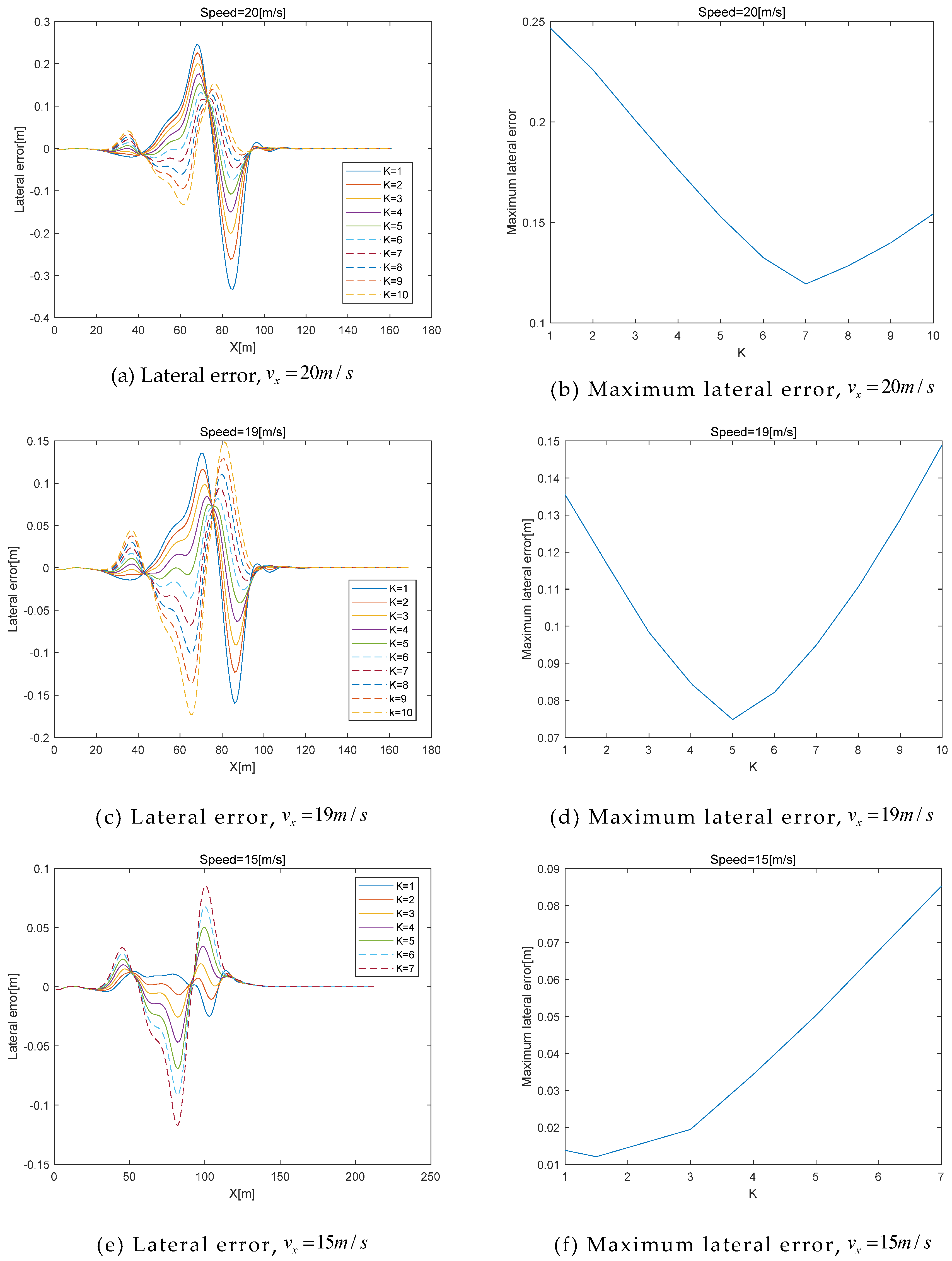
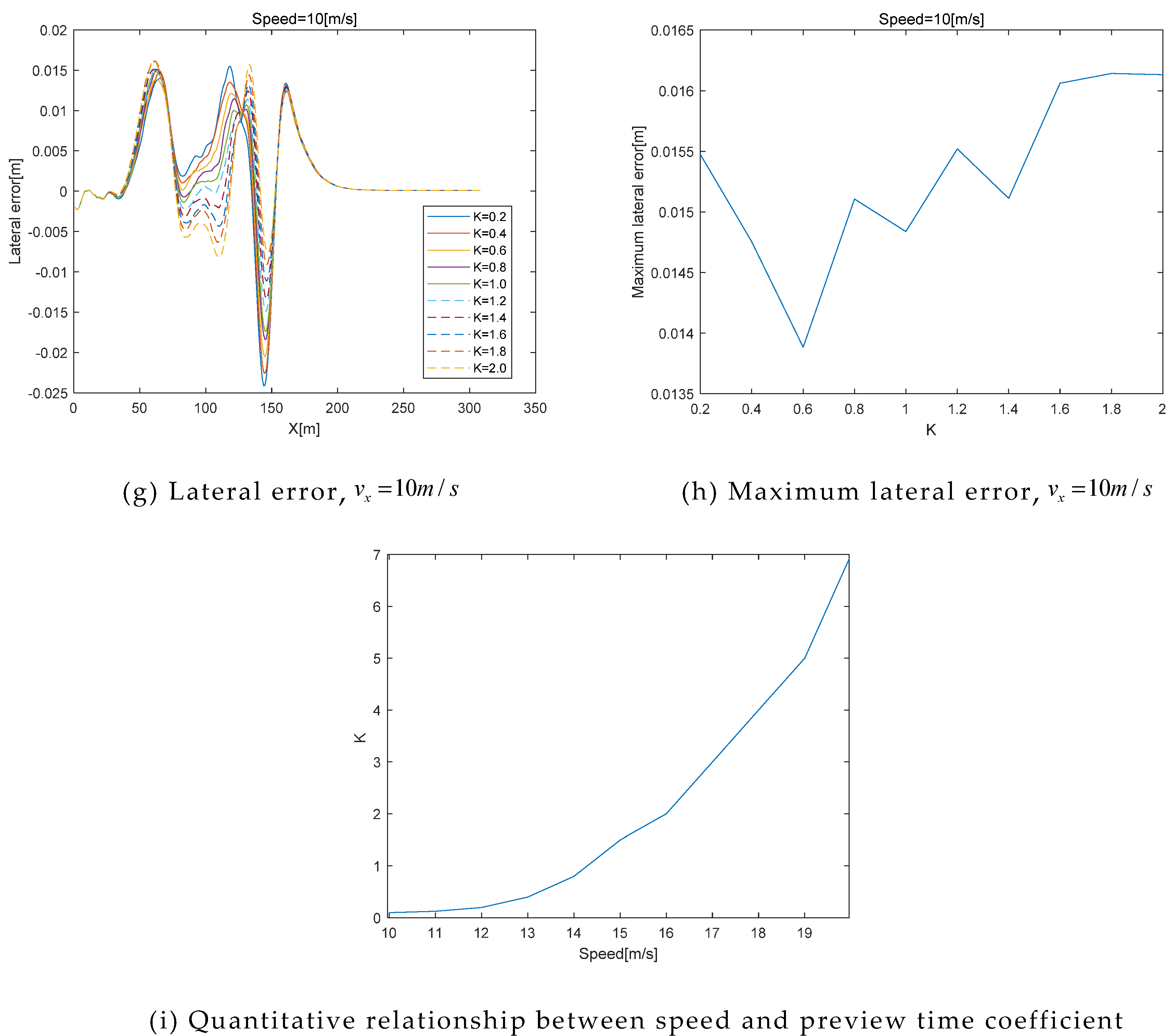
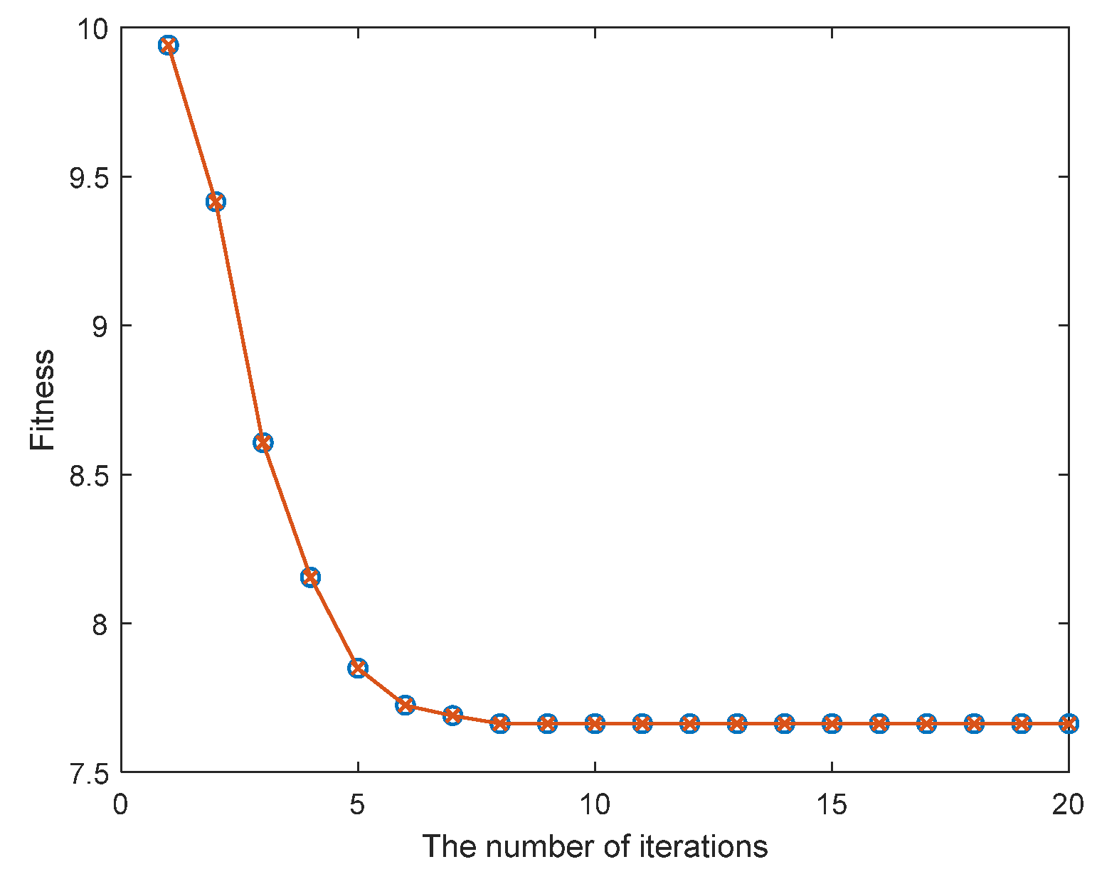
4.3. Optimal Preview Time

Due to the online real-time performance of unmanned vehicles, the optimal preview time cannot be obtained in real-time during the driving of unmanned vehicles. In this section, the PSO algorithm will be used to obtain the optimal preview time under different speeds and curvatures, and then linear interpolation will be used to obtain the optimal preview time surface.

The value of the preview time coefficient is optimized as the PSO particle, and the horizontal error converges to the minimum. The updating method of PSO is as follows:

$$\mathrm{\Delta }{\omega }_i^{k+1}=\beta \mathrm{\Delta }{\omega }_i^k+c_1{r}_{1_i}({\omega }_i^{k-\mathrm{best}}-{\overline{\omega }}_i^k)+c_2{r}_{2_i}({\omega }_i^{g-\mathrm{best}}-{\overline{\omega }}_i^k)$$

(54)

$${\overline{\omega }}_i^{k+1}={\overline{\omega }}_i^k+\mathrm{\Delta }{\omega }_i^{k+1}$$

(55)

$$\begin{array}{l}{\omega }_i^{k+1}=g({\overline{\omega }}_i^{k+1})\\ =\left\{\begin{array}{c}2{\omega }_{{\min }_i}-{\overline{\omega }}_i^{k+1},{\overline{\omega }}_i^{k+1}<{\omega }_{{\min }_i}\\ {\overline{\omega }}_i^{k+1},{\omega }_{{\min }_i}\le {\overline{\omega }}_i^{k+1}\le {\omega }_{{\max }_i}\\ 2{\omega }_{{\max }_i}-{\overline{\omega }}_i^{k+1},{\omega }_{{\max }_i}<{\overline{\omega }}_i^{k+1}\end{array}\right.\end{array}$$

(56)

Equation (54) is used to calculate the change in parameter ${\omega }_i^k$, which ${\omega }_i^k$ is the ith particle of the kth iteration; $r_{1i}$ and $r_{2i}$ are uniform random numbers in the interval [0, 1]; $c_1$, $c_2$, and $\beta$ are default positive numbers; ${\omega }_i^{k-\mathrm{best}}$ is the locally optimal particle; ${\omega }_i^{g-\mathrm{best}}$ is the global optimal particle; ${\omega }_i^{k-\mathrm{best}}$ and ${\omega }_i^{g-\mathrm{best}}$ are calculated as follows:

$${\omega }_{k-\mathrm{best}}=\underset{{\omega }^k}{\mathrm{argmin}}\{f({\omega }^k(h))|h=1,···,l\}$$

(57a)

$${\omega }^{g-\mathrm{best}}=\underset{{\omega }^{g-\mathrm{best}}}{\mathrm{argmin}}\{f({\omega }^{k-\mathrm{best}})|k=1,···,P\}$$

(57b)

When the average lateral error is selected as the evaluation index of the path-tracking performance, the fitness function of PSO is defined as the root mean square value of the lateral position error ($e_y$), as shown in Equation (58):

$$f=\sqrt{\frac{1}{N}{\displaystyle \sum _{i=1}^N{e}_y^2(i)}}$$

(58)

In order to achieve $\beta$ compromise between the local search ability and the global search ability of the particle swarm optimization algorithm, the inertia weight A of the updating particle velocity is linearly reduced.

$$\beta ={\beta }_{\max }-({\beta }_{\max }-{\beta }_{\min })\frac{f}{P}$$

(59)

where $P$ is the maximum number of iterations. According to experience, the maximum inertia weight ${\beta }_{\max }$ is set as 0.9, and the minimum inertia weight ${\beta }_{\min }$ is set as 0.4.

Figure 4 shows the change in the fitness function value corresponding to the optimal preview coefficient with longitudinal velocity of 20 m/s obtained by using PSO. It can be seen that the optimal preview coefficient can be obtained under 20 iterations.

At the speed of 0–20 m/s, PSO was used to obtain the optimal preview time corresponding to the minimum transverse error, and linear interpolation was used to obtain the optimal preview time surface, as shown in Figure 5.

According to the speed information obtained by the sensor and the calculated road curvature, the adaptive preview regulator can obtain the optimal preview time under different working conditions according to the optimal preview time surface in Figure 5.

5. Simulation and Real Vehicle Testing

The following section compares the effects of path tracking without the longitudinal speed limit, using longitudinal speed limits for MPC, fixed preview time (P-MPC), and adaptive preview time (OP-MPC).

The reference trajectory of this paper is shown in Figure 6. It’s expressed in terms of Equations (60) and (61):

$$Y_{ref}(X)=\frac{d_{y1}}{2}[1+\tanh (z_1)]-\frac{d_{y2}}{2}[1+\tanh (z_2)]$$

(60)

$${\phi }_{ref}(X)=\arctan [d_{y1}{(\frac{1}{\cosh (z_1)})}^2(\frac{1.2}{d_{x1}})-d_{y2}{(\frac{1}{\cosh (z_2)})}^2(\frac{1.2}{d_{x2}})]$$

(61)

where $z_1=\frac{2.4}{25}(X-27.19)-1.2$, $z_2=\frac{2.4}{21.95}(X-56.46)-1.2$, $d_{x1}=25$, $d_{x2}=21.95$, $d_{y1}=4.05$, $d_{y2}=5.7$.

Figure 6a shows the coordinate position of the path, Figure 6b shows the reference heading angle, and Figure 6c shows the magnitude of the road curvature.

Table 2. Controller parameters.

Parameter	Value
Prediction time domain ($N_p$)	20
Control time domain ($N_c$)	20
The sampling period ($T_s$)	0.05 (s)
Front wheel slip angle control amount ($u$)	–35°~35°
Front wheel slip angle control increment ($\mathrm{\Delta }u$)	−0.47~0.47
Q	$\left[\begin{array}{ccc}200& 0& 0\\ 0& 100& 0\\ 0& 0& 100\end{array}\right]$
R	1000

shows the MPC controller parameters.

In the Carsim software 2023.0, the road adhesion coefficient is 0.8 and the speed is 90 km/h. Figure 7 shows the effect of path following without the longitudinal speed controller (case 1), MPC (case 2), P-MPC (case 3), and OP-MPC (case 4).

Lateral error and heading error are defined according to Equation (62) and Equation (63), respectively:

$$er{r}_1=\sqrt{(x-x_0)+(y-y_0)}$$

(62)

$$er{r}_2=\phi -{\phi }_0$$

(63)

where $x$, $y$, and $\phi$ represent the current state quantity of the vehicle, which $x_0$,$y_0$, and ${\phi }_0$ are the path reference points.

In the simulation results of case 1, it can be seen from Figure 7d that when the vehicle speed is 25 m/s, the vehicle has exceeded the safe speed limit of the longitudinal speed controller, and the tracking performance and driving stability of the vehicle are reduced. It can be seen from Figure 7b that the maximum lateral error of the unmanned vehicle exceeds 2 m, and the path following fails.

In the simulation results of case 2, it can be seen from Figure 7b,f that the longitudinal speed controller limits the vehicle to a safe speed, and the maximum lateral error of the unmanned vehicle is 0.522 m, which is within an acceptable range. The steering angle of the front wheels of the vehicle changes smoothly under the constraints, and the path tracking is successful.

In the simulation results of case 3, it can be seen from Figure 7e that the MPC path-following method with fixed preview time is added on the basis of the longitudinal speed controller, and the steering angle of the front wheel can be controlled in advance under the variable-curvature path, so as to achieve early turning. The lateral error of unmanned vehicles is at most 0.437 m (Figure 7b). Compared with the method without preview time, this method improves the path-tracking accuracy.

In the simulation results of case 4, as shown in Figure 7f, the adaptive preview time can automatically adjust the preview time according to the curvature and reduce the lateral error and heading error in the current control time (Figure 7b,c). The path-following performance of this method is better than that of the fixed look-ahead time method.

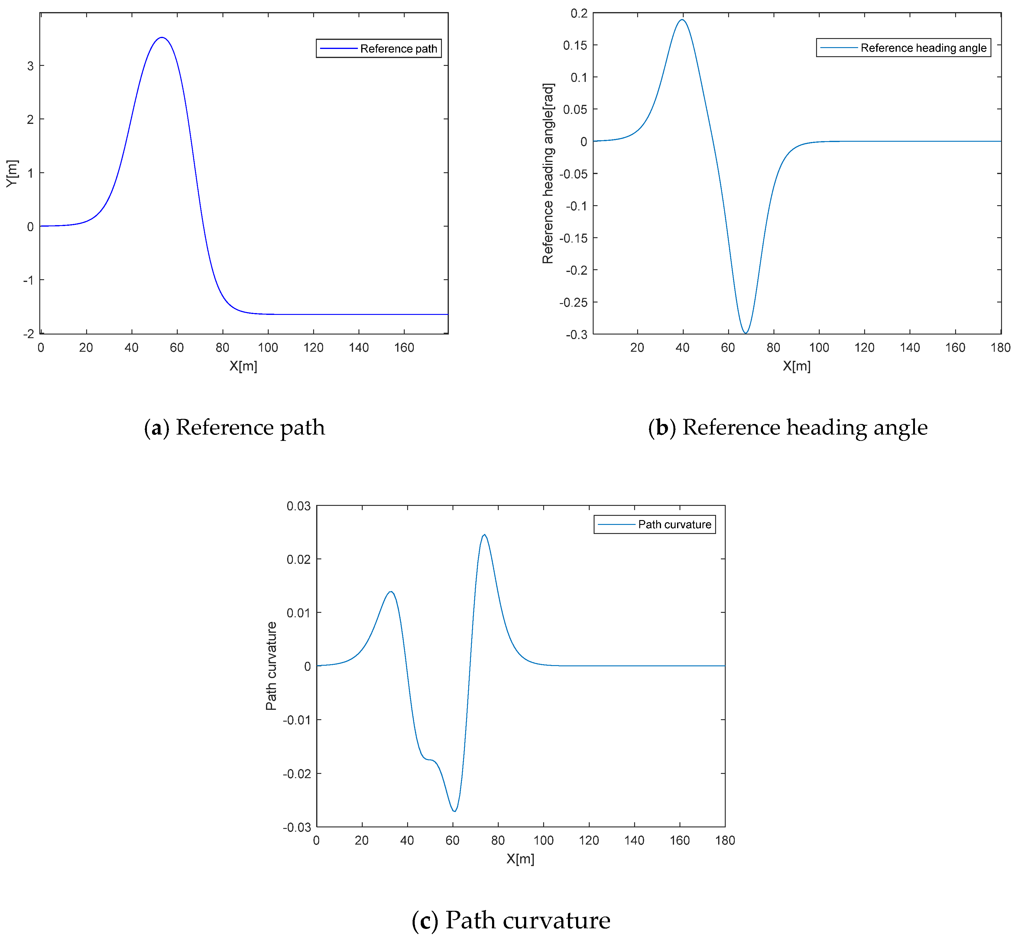
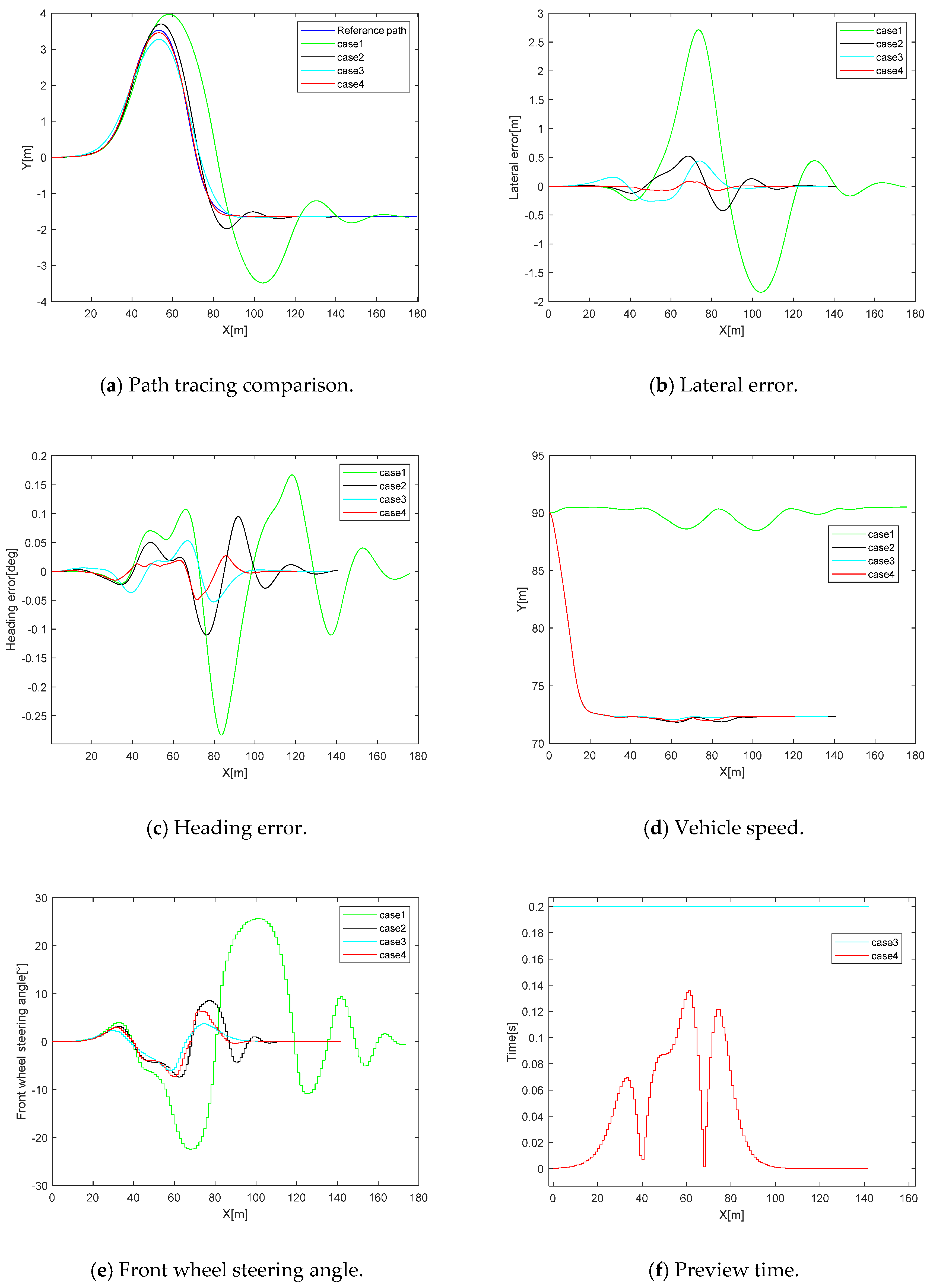
5.1. Simulation Analysis

In the above simulation results, according to Figure 7b, it can be seen that the longitudinal speed controller can effectively improve the accuracy of vehicle trajectory tracking. The maximum lateral position deviation without the longitudinal speed controller (case 1) is 2.709 m, while the active safety controller is added. The maximum lateral position deviation of the detector (case 2) is 0.522 m, the maximum lateral position deviation of the fixed preview time (case 3) is 0.437 m, and the maximum lateral position deviation of the adaptive preview time (case 4) is 0.085 m. According to Figure 7c, the maximum heading deviation without the longitudinal speed controller (case 1) is 16.044°, while the maximum heading deviation with the longitudinal speed controller (case 2) is 6.303°, the maximum heading deviation of fixed preview time (case 3) is 3.036°, and the maximum heading deviation of the adaptive preview time (case 4) is 2.809°. Compared with no preview time, the adaptive preview time improves the tracking accuracy by 72.2%. Compared with the fixed preview time, the adaptive preview time improves the tracking accuracy by 66.8%. In sum, the adaptive preview time can effectively improve the path-tracking accuracy of unmanned vehicles.

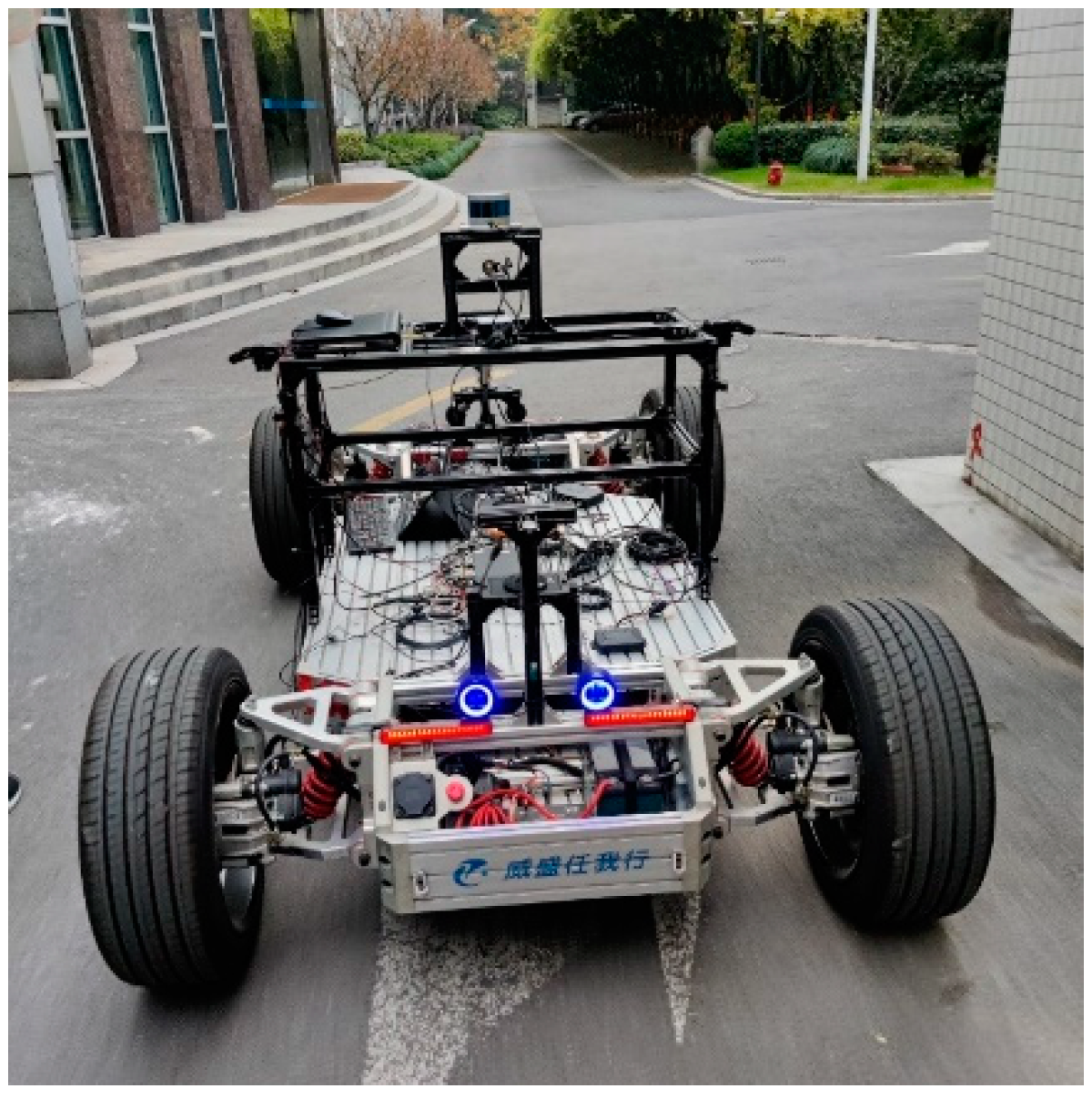
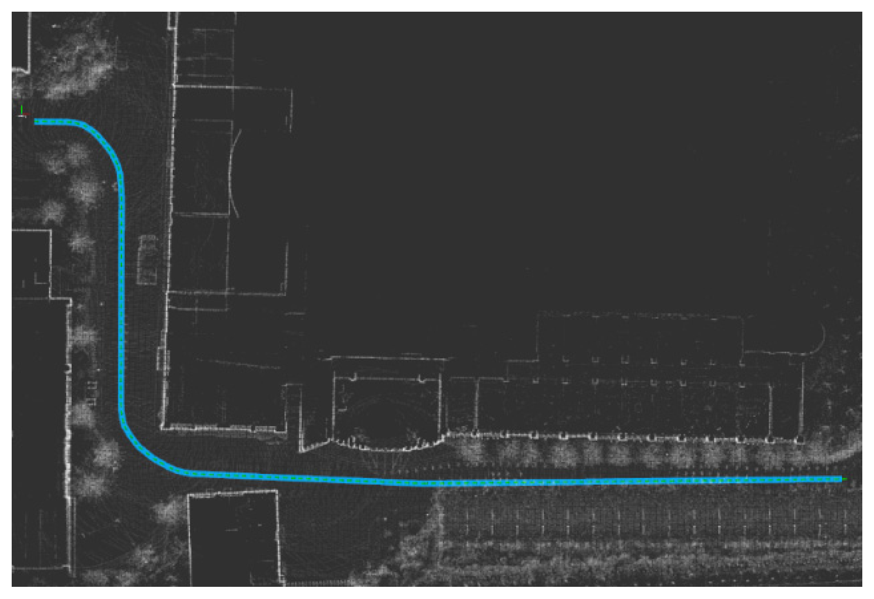
5.2. Real Car Verification

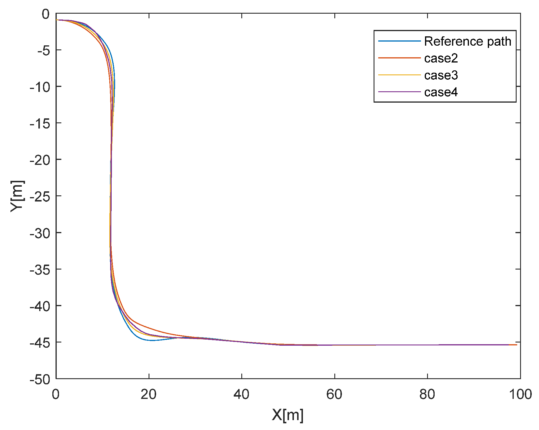
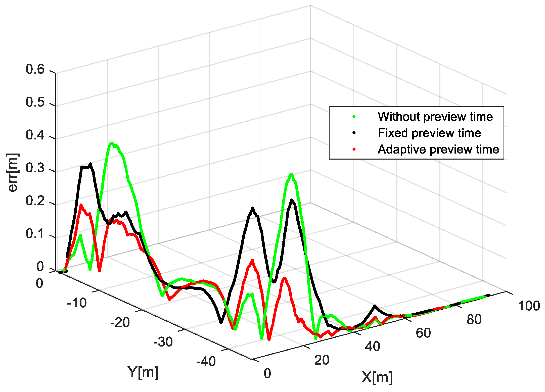
To demonstrate the effectiveness and real-time performance of the proposed control strategy, we conducted practical verification of the proposed control strategy using a real unmanned vehicle based on Lidar localization. In this study, the MPC algorithm was written to the industrial computer using C++ under the Autoware framework based on ROS1. The unmanned vehicle used in this paper, the industrial computer, and the wire-controlled chassis use CAN communication to control the steering and speed of the wire-controlled chassis of the unmanned vehicle. The ROS multi-machine communication framework was used to monitor the driving state and path-tracking performance of the vehicle in real time.

Figure 8 shows the experimental vehicle used in this paper, equipped with Lidar, a GNSS sensor, a drive-by-wire chassis, and an industrial computer. Figure 9 shows the reference path in the point cloud map.

Figure 10 shows the experimental comparison results of MPC and MPC based on adaptive preview time. According to the experimental results, the proposed control method can obviously control the lateral error under the conditions of small curve and variable curvature, and the error is within the acceptable range. There are still some differences between the simulation and the experimental results. This is because the simplified models in this paper, introduce errors, reducing their overall applicability to real driving situations.

It can be seen from Figure 11 that, in the real vehicle experiment, the maximum lateral error of no preview time was 0.5185 m, and the maximum lateral error of fixed preview time was 0.4289 m. Compared with no preview time, the tracking accuracy of fixed preview time was improved by 17.28%. The maximum lateral error of the optimal preview time was 0.2298 m, which improved the tracking accuracy by 55.67% compared with the fixed preview time.

5.3. Results

To evaluate the performance of the proposed control scheme and the improvement brought by preview time, we compared the control effects of different controllers as shown in

Table 3. Experimental tracking situation.

Experiment Number	Experimental Situation	Initial Velocity	Maximum Lateral Deviation (m)	Maximum Heading Deviation (°)
Case 1	Without the longitudinal speed controller	25 m/s	2.709	16.044
Case 2	The longitudinal speed controller	25 m/s	0.522	6.303
Case 3	Fixed preview time	25 m/s	0.437	3.036
Case 4	Adaptive preview time	25 m/s	0.145	2.809

. It can be clearly observed that the control scheme with the optimal preview time is the best. Using the longitudinal speed limit, the reference path can be tracked by the unmanned vehicle and the fixed preview time is adopted based on the use of the longitudinal speed controller, which will further improve the path-tracking performance. In the simulation test, the path-tracking accuracy could be improved by 72.2% by using the MPC controller with the optimal preview time compared with the normal MPC controller.

This improvement is also shown in Figure 7b, where four path-tracking scenarios are compared. The results show that case 4 has the best improvement in path-tracking performance, which indicates that the MPC controller based on adaptive preview time can achieve better path-tracking accuracy.

This paper studies the maximum longitudinal speed that the vehicle can achieve under variable curvature conditions to prevent the vehicle from slipping and rolling over, as shown in Figure 1, which shows the longitudinal safe speed limit for paths with different curvatures and adhesion coefficients.

Then, we investigated the influence of preview time on tracking accuracy, as shown in Figure 3, which shows the changing relationship between vehicle longitudinal velocity, path curvature, and look-ahead time. The results show that the preview time is positively correlated with the vehicle’s longitudinal velocity and the path curvature. According to the optimal preview time of the variable-curvature path-tracking process under different vehicle speeds, the surface relationship between the vehicle speed, the path curvature, and the preview time is shown in Figure 5.

Finally, this paper verified OP-MPC in the simulation test and the actual unmanned vehicle, and we found that OP-MPC can effectively improve the path-tracking accuracy.

Overall, the results show that the proposed OP-MPC controller is able to improve path-tracking accuracy under variable path curvature conditions while maintaining safe operation all the time.

6. Conclusions

This paper proposes a path-following control strategy for unmanned vehicles based on optimal preview time, model predictive control, and longitudinal speed limits. The longitudinal speed controller is designed to improve the safety and lateral stability of unmanned vehicles and prevent sideslip and rollover. The model predictive control based on the optimal preview time (OP-MPC) can effectively improve the path-tracking performance under the condition that the constraints are satisfied. In this study, the algorithm was verified on the Carsim-Simulink simulation platform. Under the condition of variable curvature, the path-following accuracy of the OP-MPC method was improved by 66.8% compared with the MPC with fixed preview time MPC (P-MPC). The OP-MPC method was tested on an actual unmanned vehicle, and the path-following accuracy of the OP-MPC method was improved by 55.67% compared with MPC with fixed preview time (P-MPC). In an actual unmanned vehicle, the effectiveness of the control strategy was verified. The experimental results show that the control method has good control ability and satisfactory performance under the condition of variable path curvature, but the simplified models reduce its overall applicability to real driving situations.

References

1. König, M.; Neumayr, L. Users’ resistance towards radical innovations: The case of the self-driving car. Transp. Res. Part F Traffic Psychol. Behav. 2017, 44, 42–52. [Google Scholar] [CrossRef]
2. Paden, B.; Čáp, M.; Yong, S.Z.; Yershov, D.; Frazzoli, E. A survey of motion planning and control techniques for self-driving urban vehicles. IEEE Trans. Intell. Veh. 2016, 1, 33–55. [Google Scholar] [CrossRef]
3. Dudziak, A.; Stoma, M.; Kuranc, A.; Caban, J. Assessment of Social Acceptance for Autonomous Vehicles in Southeastern Poland. Energies 2021, 14, 5778. [Google Scholar] [CrossRef]
4. Li, X.; Sun, Z.; Cao, D.; Liu, D.; He, H. Development of a new integrated local trajectory planning and tracking control framework for autonomous ground vehicles. Mech. Syst. Signal Process. 2017, 87, 118–137. [Google Scholar] [CrossRef]
5. Kayacan, E.; Ramon, H.; Saeys, W. Robust trajectory tracking error model-based predictive control for unmanned ground vehicles. IEEE/ASME Trans. Mechatron. 2015, 21, 806–814. [Google Scholar] [CrossRef]
6. Tian, Y.; Huang, K.; Cao, X.; Liu, Y.; Ji, X. A hierarchical adaptive control framework of path tracking and roll stability for intelligent heavy vehicle with MPC. Proc. Inst. Mech. Eng. Part D J. Automob. Eng. 2020, 234, 2933–2946. [Google Scholar] [CrossRef]
7. Sun, C.; Zhang, X.; Zhou, Q.; Tian, Y. A model predictive controller with switched tracking error for autonomous vehicle path tracking. IEEE Access 2019, 7, 53103–53114. [Google Scholar] [CrossRef]
8. Du, X.; Htet, K.K.K.; Tan, K.K. Development of a genetic-algorithm-based nonlinear model predictive control scheme on velocity and steering of autonomous vehicles. IEEE Trans. Ind. Electron. 2016, 63, 6970–6977. [Google Scholar] [CrossRef]
9. Falcone, P.; Borrelli, F.; Asgari, J.; Tseng, H.E.; Hrovat, D. Predictive active steering control for autonomous vehicle systems. IEEE Trans. Control Syst. Technol. 2007, 15, 566–580. [Google Scholar] [CrossRef]
10. Bai, G.; Liu, L.; Meng, Y.; Luo, W.; Gu, Q.; Ma, B. Path tracking of mining vehicles based on nonlinear model predictive control. Appl. Sci. 2019, 9, 1372. [Google Scholar] [CrossRef]
11. Xu, S.; Peng, H. Design, analysis, and experiments of preview path tracking control for autonomous vehicles. IEEE Trans. Intell. Transp. Syst. 2019, 21, 48–58. [Google Scholar] [CrossRef]
12. Sun, C.; Zhang, X.; Xi, L.; Tian, Y. Design of a path-tracking steering controller for autonomous vehicles. Energies 2018, 11, 1451. [Google Scholar] [CrossRef]
13. Guo, H.; Liu, J.; Cao, D.; Chen, H.; Yu, R.; Lv, C. Dual-envelop-oriented moving horizon path tracking control for fully automated vehicles. Mechatronics 2018, 50, 422–433. [Google Scholar] [CrossRef]
14. Ji, X.; He, X.; Lv, C.; Liu, Y.; Wu, J. Adaptive-neural-network-based robust lateral motion control for autonomous vehicle at driving limits. Control Eng. Pract. 2018, 76, 41–53. [Google Scholar] [CrossRef]
15. Yang, L.; Yue, M.; Ma, T. Path following predictive control for autonomous vehicles subject to uncertain tire-ground adhesion and varied road curvature. Int. J. Control Autom. Syst. 2019, 17, 193–202. [Google Scholar] [CrossRef]
16. Bai, G.; Meng, Y.; Liu, L.; Luo, W.; Gu, Q.; Li, K. A new path tracking method based on multilayer model predictive control. Appl. Sci. 2019, 9, 2649. [Google Scholar] [CrossRef]
17. Yu, R.; Guo, H.; Sun, Z.; Chen, H. MPC-based regional path tracking controller design for autonomous ground vehicles. In Proceedings of the 2015 IEEE International Conference on Systems, Man, and Cybernetics, Hong Kong, China, 9–12 October 2015; pp. 2510–2515. [Google Scholar]
18. Cao, H.; Song, X.; Zhao, S.; Bao, S.; Huang, Z. An optimal model-based trajectory following architecture synthesising the lateral adaptive preview strategy and longitudinal velocity planning for highly automated vehicle. Veh. Syst. Dyn. 2017, 55, 1143–1188. [Google Scholar] [CrossRef]
19. Yang, W.; Li, C.; Zhou, Y. A Path Planning Method for Autonomous Vehicles Based on Risk Assessments. World Electr. Veh. J. 2022, 13, 234. [Google Scholar] [CrossRef]
Figure 1. Longitudinal speed limit.
Wevj 15 00221 g001
Figure 2. Vehicle model.
Wevj 15 00221 g002
Figure 3. Comparing the corresponding lateral error changes at different vehicle speeds. (a) Lateral error, v x = 20   m / s ; (b) Maximum lateral error, v x = 20   m / s ; (c) Lateral error, v x = 19   m / s ; (d) Maximum lateral error, v x = 19   m / s ; (e) Lateral error, v x = 15   m / s ; (f) Maximum lateral error, v x = 15   m / s ; (g) Lateral error, v x = 10   m / s ; (h) Maximum lateral error, v x = 10   m / s ; (i) Quantitative relationship between speed and preview time coefficient.
Wevj 15 00221 g003aWevj 15 00221 g003b
Figure 4. PSO iterations at a speed of 20 m/s.
Wevj 15 00221 g004
Figure 5. Optimal preview time surface.
Wevj 15 00221 g005
Figure 6. Reference Path. (a) Reference path; (b) Reference heading angle; (c) Path curvature.
Wevj 15 00221 g006
Figure 7. Comparison of path tracking effects at 90 km/h. (a) Path tracing comparison; (b) Lateral error; (c) Heading error; (d) Vehicle speed; (e) Front wheel steering angle; (f) Preview time.
Wevj 15 00221 g007
Figure 8. Experimental vehicle.
Wevj 15 00221 g008
Figure 9. Experimental scene.
Wevj 15 00221 g009
Figure 10. Reference path.
Wevj 15 00221 g010
Figure 11. Comparison of lateral errors.
Wevj 15 00221 g011