Abstract
The strategic development of reverse logistics networks is crucial for addressing the common challenge of low recovery rates for end-of-life vehicles (ELVs) in China. To minimize the total cost of the reverse logistics network for ELVs, this paper proposes a mixed-integer linear programming (MILP) model. The model considers the recycling volume of different vehicle types, facility processing capacity, and the proportions of parts and materials. Building on this foundation, a fuzzy mixed-integer nonlinear programming (FMINLP) model is developed to account for the inherent uncertainty associated with recycling volumes and facility processing capacities. The model was solved using Lingo, and its effectiveness was validated using Jiangsu Province of China as a case study, followed by a sensitivity analysis. The results indicate that dismantling and machining centers incur the highest processing costs. Variations in recycling volume and facility handling capacity significantly impact total costs and site selection, with the former having a more pronounced effect. Increasing facility processing capacity effectively increases the recovery rate. Moreover, a higher confidence level corresponds to higher total costs and a greater demand for facilities.
1. Introduction
With the continuous improvement of environmental requirements worldwide and the increasing recognition of recyclable and valuable materials in discarded products [1], reverse logistics has become fully developed on a global scale. Reverse logistics involves logistics activities related to waste disposal, recycling, and hazardous material management [2]. Reverse logistics for end-of-life vehicles (ELVs) has become an important part of waste management due to the rapid growth in the number of automobiles and their limited lifespan. Currently, waste from the automotive industry accounts for about 5% of the world’s industrial waste. ELVs contain many materials that can impact the environment, and improper disposal can lead to environmental pollution [3,4]. However, the proper recycling and reuse of components and metal materials from ELVs can generate significant production value [5]. Therefore, reverse logistics for ELVs not only benefits environmental protection and resource conservation but also promotes economic growth.
The number of ELVs in China has continuously increased, from 4.81 million in 2014 [6] to 16.8 million in 2023 [7]. However, the management of recycling operations is poor, and the layout of reverse logistics networks is immature. Additionally, there is uncertainty in the processing capacity of enterprises, with most dismantling companies having low recycling volumes. The amount of ELVs entering formal recycling channels accounts for only about 20% of the actual ELVs [8]. The low recycling volume of ELVs can easily cause environmental pollution. China has found through pilot projects in economically developed cities that implementing ELV management can effectively achieve sustainable development [9]. Establishing an effective reverse logistics network for ELVs will help solve resource allocation issues in the recycling process, provide decision-makers with optimal solutions for the actual operation of recycling systems, and promote the effective reuse of recycled resources.
The research on the reverse logistics network of ELVs began in the early 21st century [10], when researchers put forward a variety of methods for modeling and solving existing cases. Cruz-Rivera and Ertel [11] designed a reverse logistics network for ELVs in Mexico. Demirel et al. [12] proposed a mixed-integer linear programming (MILP) model, where network nodes include end-users, recycling centers, dismantling centers, shredding centers, landfills, and second-hand markets. On this basis, Özceylan et al. [13] designed a closed-loop supply chain network structure, where reusable parts, after processing, are sold to suppliers for remanufacturing and finally to consumers. Phuc et al. [14] designed a testing center in the network, and the ELVs that were inspected were repaired and sold to the second-hand market. Simic and Dimitrijevic [15] used waste incinerators and heat treatment measures to treat automobile shredder residue (ASR). Most of the current research focuses on building single-objective MILP models to minimize total cost or maximize profit [16]. In addition, most scholars conduct analyses through numerical examples, and there are few studies on the construction and optimization of reverse logistics networks in specific areas. Specific examples are relatively scarce.
In addition, uncertainty is a key factor affecting ELV management [17], but there are few related studies. Most of these studies use a method based on scenario analysis and do not consider the uncertainty factors of reverse logistics networks when building the model, which leads to the discrepancy between the model and the actual situation. This discrepancy makes it difficult to ensure the robustness of the network. Only a few studies have used fuzzy programming to resolve uncertainty and modeled the uncertainty of price parameters, such as processing cost, sales price, and transportation cost [14,17,18]. However, few studies have considered the uncertainty of the number of ELVs [19]. Scientifically forecasting the recycling quantity of ELVs can effectively help address uncertainties in actual recycling. The existing literature typically adopts single forecasting models, including statistical models based on life distribution and grey models, which may impact the accuracy of predictions. Addressing some shortcomings in the current construction of reverse logistics networks for ELVs, this paper aims to solve the following issues. Firstly, it aims to achieve accurate forecasting of future annual ELV recovery volumes by improving the prediction model. Secondly, it responds to uncertainties in the process of ELV recovery by proposing a new reverse logistics network planning model. This model aims to minimize the total network cost and generate site selection decisions and transportation plans. Finally, the proposed model will be applied to real-world scenarios to demonstrate its effectiveness and practicality. Overall, this paper makes the following contributions:
- Recycling prediction is an important topic for addressing recycling uncertainty. This paper constructs a forecasting model for ELV recycling by combining the grey model, exponential smoothing, and the Markov model. It effectively handles the influence of nonlinearity, randomness, and related fluctuations on the prediction results. Compared with traditional single forecasting methods, it improves the accuracy of predictions.
- Distinguished from existing research, this paper constructs a multi-level reverse logistics network for ELVs. It proposes a mixed integer linear programming (MILP) model that simultaneously considers the quantity of recovered vehicles for different types and the capacity of processing facilities. Considering the uncertainty in the quantity of ELV recovery and facility handling capacity, a fuzzy planning approach is introduced to construct a fuzzy mixed integer nonlinear programming (FMINLP) model, which is more practical.
In summary, this paper constructs a combined forecasting method for the quantity of ELV recovery and proposes a novel modeling approach for reverse logistics planning. In doing so, it fills a research gap in the field regarding uncertainty and practical applications. This contribution is significant for both academia and practice. The research findings can serve as a reference for policy-making related to ELV recycling, contributing to the efficiency and sustainability of the recycling industry.
The following chapters are structured as follows. Section 2 provides a review of relevant literature. Section 3 presents the problem description of this study. Section 4 introduces the methods used and the mathematical model constructed in this study. Section 5 presents a practical case study from Jiangsu Province of China, and analyzes the results of the solution. Section 6 further discusses the integrated solution results and sensitivity analysis, providing relevant management and policy recommendations. Finally, Section 7 concludes this paper.
2. Literature Review
The construction of a reverse logistics network includes determining the location and quantity of network entities and analyzing the spatial distribution of logistics, ensuring that waste flows smoothly from consumers back to manufacturers. This kind of problem belongs to the design problem at the strategic level [20]. The research on the reverse logistics network of ELVs has now become the focus of attention. This paper compiles literature that is highly related to the construction of reverse logistics networks for ELVs from previous studies, as shown in Table 1.

Table 1.
Literature summary of reverse logistics network construction of ELVs.
Through a comprehensive comparison of this literature, it can be observed that most of the reverse logistics networks for ELVs are designed as open-loop supply chains, operated by third-party enterprises for recycling. The majority of the literature constructs single-objective models with little consideration for uncertainties. Small to medium-scale cases are typically solved using exact methods, with Lingo and CPLEX being the primary tools used for finding solutions. All single-objective models consider economic benefits, aiming to minimize costs (usually including acquisition costs, facility fixed and variable costs, transportation costs, and in some cases, carbon emission costs) or maximize profits (revenue from parts and materials sales minus costs). On the other hand, multi-objective models integrate economic, social, and environmental benefits. For large-scale problems and nonlinear models, scholars have gradually proposed heuristic algorithms to improve solution efficiency, including particle swarm algorithms, improved artificial bee colony algorithms, and taboo search algorithms. Additionally, most studies focus on case analyses, with limited research on the construction and optimization of reverse logistics networks for specific regions, resulting in a scarcity of specific practical applications.
2.1. Model Construction and Algorithm Solution
In the field of model construction and algorithm solution for the reverse logistics network of ELVs, the main focus of most scholars is how to construct the reverse logistics network and related mathematical models. Ene and Öztürk [35] designed a reverse logistics network consisting of recycling, dismantling, processing, and machining centers, constructed an MILP model aiming at maximizing profit and solved it with Lingo 17.0 software, and finally concluded that recycling and remanufacturing activities have huge profits. Ahmed and Ali [36] constructed a single-objective multi-cycle MILP model, aiming at maximizing the total profit and calculating the maximum profit of the reverse logistics network of ELVs under different conditions. Xiao et al. [20] constructed a four-layer reverse logistics network model including consumers, recycling centers, remanufacturing centers, and dismantling centers. In this model the logistics and environmental costs are reduced, and the utilization rate of the dismantling center is improved. Taking into account environmental and social impacts, Budak [28] constructed a model to minimize the total economic cost of the reverse logistics network and used an improved augmented epsilon constraint algorithm to select the locations of storage centers, recycling centers, and dismantling centers in Turkey. Based on the characteristics of big data, Govindan and Gholizadeh [29] verified the effectiveness of the algorithm by applying a scenario-based cross-entropy algorithm to cases of different scales.
The above researchers all use the MILP model to describe the reverse logistics network of ELVs, with some researchers using more complex mathematical methods to make the constructed model more realistic. Govindan et al. [37] constructed a fuzzy multi-objective multi-period model aimed at maximizing profit. The model seeks to find the Pareto optimal solution for the three objectives. Sun et al. [27] decomposed the location problem of the parts distribution centers into two layers. The upper layer determines the location of the distribution center, while the lower layer represents the distribution route under the location mode. This approach allows them to obtain a compromise result between the location cost of the distribution center and the transportation cost. Hashemi [30] constructed a fuzzy multi-objective model that minimizes environmental costs and the total cost of the reverse logistics network and maximizes customer demand. He used a genetic algorithm with an elite strategy and a meta-heuristic bee colony algorithm to solve the model. The performance of the two algorithms was compared to determine their effectiveness. Reddy et al. [33] developed and applied the improved benders decomposition method. It solves the MILP model, provides a faster solution, improves the convergence boundary, and solves the inherent complexity of existing problems. Reddy et al. [33] considered four green technologies and proposed a multi-objective mixed integer programming model for configuring reverse logistics network design.
Some researchers combine forward logistics and reverse logistics to form a closed-loop supply chain. Yi et al. [38] considered the supplier as one of the logistics network nodes. They used the genetic algorithm to solve the forward logistics model and the mathematical programming method to solve the reverse logistics model, obtaining a method for solving the closed-loop supply chain model. Rodolfo and Carlos [39] designed a closed-loop supply chain system for ELVs and constructed a multi-cycle and multi-level MILP model. Kumar et al. [40] designed a closed-loop supply chain and constructed a multi-period and multi-level model using mixed integer non-linear programming (MINLP). They solved the model using the simulated annealing algorithm.
Based on the above research, it can be seen that a large number of scholars have conducted a wide range of research in this field. The mathematical model has changed from simple to complex, and the solution method has gradually changed from precise algorithms to advanced heuristic algorithms.
2.2. Reverse Logistics Network Design
In the field of reverse logistics network design for ELVs, researchers are more and more concerned with addressing uncertainty [14,41]. Cruz-Rivera and Ertel [11] take Mexico as an example to build a reverse logistics network for ELVs and solve the uncertainty of collection coverage by considering three cases: 100%, 90%, and 75% coverage rates, respectively. Demirel et al. [12] predicted the long-term average development of the number of ELVs in Ankara, the capital of Turkey. They determined the number of facilities that need to be located, and found that the system cost increases with the number of ELVs in the future. Özceylan et al. [13] analyzed the impact of uncertainty on total network returns through several closed-loop supply chain scenarios for ELVs, including changes in recycling rates, the ratio of vehicle sales prices to manufacturing costs, the number of dismantling centers, and carbon emission limits.
There are also a few scholars using fuzzy methods to solve the uncertainty in the reverse logistics network of ELVs. Phuc et al. [14] believed that a fuzzy environment prevailed for various parameters, and adopted a comprehensive fuzzy method. Simic [42] constructed a fuzzy linear programming model considering uncertainties related to transportation and processing costs and scrap prices. Kuşakcı et al. [19] established a FMINLP model that complies with the current Turkish directive, considering the uncertainty of the number of ELVs recycled. Hashemi [30] asserts that the construction cost of each facility in the reverse logistics network and consumers’ recycling demands are uncertain. To address this uncertainty, a fuzzy model is refined by the method of triangular fuzzy numbers. Wenzhu Liao and Luo [32] examined two types of waste electric vehicle batteries, designed a multi-level reverse logistics network of waste batteries according to the different flow directions of the disassembled parts, proposed a fuzzy optimization model, and applied the model to a practical case at Chongqing Chang’an Automobile Company in China.
In addition, the prediction of the number of ELVs recycled can help to solve the uncertainty problem in recycling and play an important role in building a reasonable reverse logistics network [43]. Soki et al. [44] used a two-parameter Weibull distribution function to simulate the frequency distribution of the number of ELVs in Serbia in the future. Ene and Öztürk [33] used a grey model to predict the number of ELVs in the future and improved the prediction accuracy through parameter optimization and Fourier series correction. Xin et al. [45] proposed two methods, generalized regression neural network, and artificial bee colony-based optimization, to predict the number of ELVs. Yi Man Li et al. [46] also used an automated machine learning method—a modification heuristic algorithm—to forecast parking lot prices in Hong Kong, China. Yu et al. [47] established a logistics distribution function and used a statistical model to predict and analyze the future trend of the number of ELVs in China. Zhang et al. [48] proposed a multi-time scale attention network model to predict the recycling of waste electrical and electronic equipment.
This paper addresses deficiencies in the current construction of the reverse logistics network for ELVs, particularly the lack of research on uncertainty. Firstly, it constructs a combined forecasting model to predict the recycling levels of China’s ELVs. Secondly, it develops an FMINLP model for the reverse logistics network of ELVs and conducts an in-depth analysis of uncertain factors. Finally, the model is applied to determine the locations of reverse logistics facilities in Jiangsu Province, China.
3. Problem Description
The reverse logistics network of ELVs consists of a variety of facilities with different functions. The network structure in this paper, shown in Figure 1, contains ELVs areas (), recycling centers (), dismantling centers (), machining centers (), processing centers (), remanufacturing centers (), second-hand markets (), loop centers (), and landfills ().
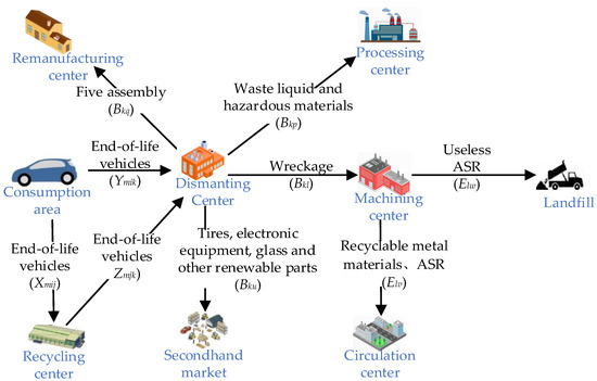
Figure 1.
Reverse logistics network of ELVs.
Recycling centers purchase ELVs from consumers and transport them to dismantling centers. At the dismantling center, the initial operation involves draining fluids and removing hazardous components, with the resulting liquids and materials being sent to a processing center. ELVs are then dismantled on a dismantling line, with major components, such as hubs and differentials, directed to a remanufacturing center, while the metal parts and tires are sent to the second-hand market. The remaining components are compressed and forwarded to machining centers. At the machining center, materials undergo mechanical recovery using equipment such as pulverizers, suction fans, magnetic separators, and eddy current separators. This process separates materials into ferrous metals, non-ferrous metals, and ASR. Following compression, the materials are sent to circulation centers for remanufacturing, while any remaining unusable ASR is sent to landfills.
The objective of this paper is twofold. Firstly, it aims to enhance the precision of ELVs recycling level prognostication and facilitate the design of a reverse logistics network through the formulation of an integrated forecasting model for ELVs recycling. Secondly, it aims to determine the locations of recycling centers, dismantling centers, and machining centers within the reverse logistics network with the lowest investment costs. The geographical locations of other facilities within this area have already been determined, and this paper also seeks to establish the logistics flow between these facilities. Furthermore, real-world data is often partial and uncertain. Data-driven decisions can be addressed using fuzzy sets and related systems [49]. This study considers the uncertainties in both the quantity of ELV recovery and processing capacity of facilities, treating them as fuzzy parameters, and thus introduces the fuzzy programming approach.
When developing the foundational model, the following assumptions are considered:
- Ignore differences in the level of remanufacturing and reuse of components caused by differences in the condition of ELVs.
- The number of ELVs in the consumption area is obtained by forecasting.
- The locations of the alternative recycling centers, dismantling centers, and machining centers are identified and known.
- Regardless of the dynamics existing in the network, logistics and remanufacturing activities are considered instantaneous.
4. Materials and Methods
4.1. ELVs Recycling Quantity Prediction Model
The uncertainties in ELVs, such as recycling time, quality, and policies, affect the accuracy of recycling predictions. Traditional statistical analysis models require a large sample size, which is not feasible due to the limited data availability in this study. Therefore, the grey model is used for initial data processing [50]. The Markov model performs well in predicting changes with large fluctuations in observed values, which helps improve the accuracy of single prediction models with low accuracy [51]. Therefore, this study adopts a weighted Markov model correction based on grey theory to reduce the impact of uncertainty and effectively improve prediction accuracy.
4.1.1. Principle of the Weighted Markov Model
The Markov model predicts the development trend by calculating the probability of state transition. Its basic principle can be expressed as follows:
Among them, and are the state probability vectors of the sequence at time and time respectively; is the probability matrix of state transition.
The assumed state-space distribution of is as follows:
Among them, is the state interval, and are called the upper and lower bounds of the interval, is the number of state intervals. The probability of to transition from state to is [52]:
Among them, is the number of transitions from state to , is total number of times is visited.
In the weighted Markov model, unlike the traditional Markov model, which overlooks the correlation degree between states, the state transition probability matrix receives distinct weights based on varying step sizes. This approach quantitatively differentiates the strength of the relationship between the states [52].
where is the -order autocorrelation coefficient, is the Markov weight with step size , is the mean of the series, and is the grey fitting accuracy index at the period.
4.1.2. Correcting Model Prediction Results
The initial model prediction results are processed as follows:
The residual sequence , is the actual value and is the predicted value.
Thus, the relative error sequence is obtained:
Using the mean-standard deviation method to divide the state interval of sequence [53], all intervals are , , , , , , and .
Among them,
Calculate and in turn, and sum the predicted probabilities of the same state weighted. The state with the maximum value is the state of the relative error, based on which the revised prediction result is calculated:
Among them, is the revised forecast value, is the predicted value for the initial model, and is the symbolic function.
Let the initial symbolic state matrix be:
where is the probability that the error is positive, that is, the probability of being in state 1. is the probability that the error is negative.
The probability expression of the symbol state after transitions is:
Among them, is the error symbol state transition probability matrix.
4.1.3. Grey–Markov Combination Model
In this paper, combining the grey model and the Markov model, a combined model is constructed to predict the ratio of the ELV recycling quantity to the holding quantity, as shown in Figure 2.
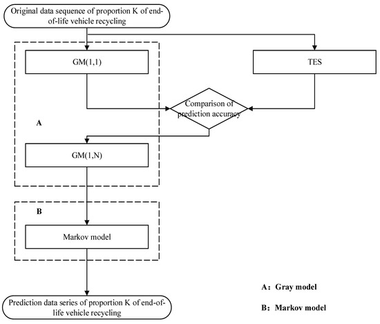
Figure 2.
A flow chart of combining grey model and Markov model.
Firstly, employ TES and GM (1, 1) to predict the respective factors influencing the time series , and compare the accuracy of the prediction results between the two. Secondly, the results with higher prediction performance are incorporated into GM (1, N) to obtain the GM (1, N) fitting value of the time series . Finally, the is corrected using the Markov model.
4.2. Reverse Logistics Network Optimization Model
The parameter and variable symbols involved in constructing the model in this chapter are shown in Table 2.
Table 2.
The sets, parameters, and variables involved in the model.
4.2.1. Basic Model
The objective function of the reverse logistics network for ELVs includes construction cost and operational cost . Operational costs comprise fixed operating costs of facilities, transportation costs, facility handling costs, and acquisition costs.
From this, the basic model can be constructed as follows:
Equation (15) is the objective function, which represents the minimum total cost. Constraints (16)–(23) represent the logistics balance between facilities, where constraint (16) indicates that all ELVs collected in the consumption area flow to both the recycling center and dismantling center. Constraint (17) represents the logistics balance of the recycling center, and Constraints (18)–(21) indicate the logistics balance of the dismantling center. Constraints (22) and (23) represent the logistics balance of the machining center. Constraints (24)–(26), respectively, indicate that the inflow of logistics to the recycling center, dismantling center, and machining center cannot exceed their maximum handling capacities. Constraint (27) restricts the decision variables to binary values (0–1). Constraints (28)–(30), respectively, indicate that the construction quantity of each facility cannot exceed the maximum quantity limit. Constraint (31) indicates that decision variables cannot be negative.
4.2.2. Fuzzy Optimization Model
Considering the uncertainty surrounding the quantity of ELVs recovered and the capacity of the facility to handle them, this paper proposes a modification to the deterministic model. Specifically, it replaces the ELV recycling amount represented by variable with a fuzzy parameter, denoted as . Recycling, dismantling, and machining center handling capacities , , are replaced by , , , respectively. The fuzzy parameters involved are dynamic and non-linear. This study models them using fuzzy programming methods [54]. The fuzzy objective function is as follows:
The fuzzy constraints are as follows:
4.2.3. Solution of Fuzzy Model
Due to the existence of fuzzy parameters , , , , it is necessary to convert an uncertain fuzzy programming model into a deterministic fuzzy programming model [30]. Since the amount of ELV recycling is a predictive parameter, is converted into a triangular fuzzy number, as shown in Figure 3, marked as . Facility handling capacity , , is a cost parameter, usually expressed by a tolerance fuzzy number, as shown in Figure 4. Take as an example, marked as . The following are membership functions for recycling volume and facility capacity:
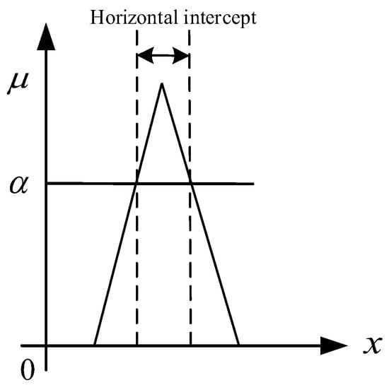
Figure 3.
Membership function of triangular fuzzy number.
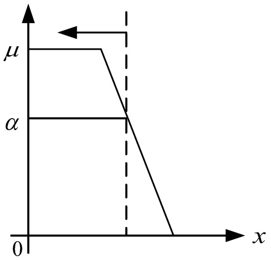
Figure 4.
Membership function of tolerance fuzzy number.
To simplify the expression, given as the form of the objective function, its membership function is the following:
where is the objective function value of the deterministic model and is the preset expansion and contraction amount.
For any given confidence level (), when the probability of the constraint taking this value is not less than the confidence level , the fuzzy optimization model can be transformed into an equivalent clear expression. Therefore, replace the Equations (32)–(36) with Equations (41)–(45), respectively. Equivalent deterministic models of fuzzy optimization models can be written. Furthermore, the original fuzzy objective function becomes a deterministic constraint with the maximization of the desired level, as shown in Equation (40). The FMINLP model is transformed into an equivalent MILP model for ease of solution, after being clarified.
The objective function defuzzification process is outlines below:
The constrained defuzzification process is as follows:
5. Case Study
By forecasting the number of ELVs to be recycled in Jiangsu Province over the next few years and using the predicted number of ELVs recovered in 2032, a reverse logistics network is constructed. The core of Lingo software used for solving the optimization problem is the branch-and-bound method, which can provide precise optimization results. It includes a powerful modeling language and a comprehensive environment for building and editing models, allowing for the rapid and effective solution of linear or nonlinear optimization models [34]. The model in this paper is a typical nonlinear programming model for location–allocation, suitable for solving with Lingo software. Therefore, this study utilized Lingo optimization software to optimize facility locations and logistics distribution plans, aiming to minimize costs and determining the optimal flow of ELVs, components, materials, and waste among facilities. The sensitivity analysis included an examination of how changes in the number of ELVs recovered and the processing capacity of facilities affect the total cost, facility location, and the logistics distribution scheme.
5.1. Determination of Candidate Site Locations and Parameters
There are currently 13 prefecture-level cities in Jiangsu Province. Compared to other provinces and cities in China, the ELV recycling market is relatively standardized, but there are also problems such as an imperfect recycling network and low recycling efficiency. Therefore, it is necessary to establish a unified recycling platform and integrate the reverse logistics network of end-of-life automobiles. By conducting pilot projects for the construction of a waste vehicle recycling network in economically developed Jiangsu Province, it can serve as a model for the scrap vehicle recycling industry in other provinces in China. Each city can utilize the existing infrastructure, such as distribution centers, to establish recycling centers. Therefore, this case does not involve the location of recycling centers, as it considers the consumption area and recycling center as the same node, focusing solely on the construction of large-scale dismantling and machining centers. The largest number of dismantling centers is 13, and the largest number of machining centers is 8. Taking into full consideration the leading industries, traffic locations, and economic conditions in each region, the candidate locations for each facility are shown in the Figure 5, and the distance between the facilities is the shortest urban road distance on the Baidu map. The number of civilian vehicles in various cities in Jiangsu Province was obtained by consulting the Jiangsu Statistical Yearbook.
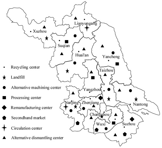
Figure 5.
Administrative divisions and facility node distribution in Chinese Jiangsu Province.
and represent the fixed construction cost and annual operating cost of the dismantling center, respectively. and represent the fixed construction cost and annual operating cost of the machining center, respectively.
By researching the literature [19], the relevant costs and maximum processing capacity of alternative facilities were determined. The unit handling cost of dismantling center and processing center is 300 and 400 respectively. The fixed construction cost and the annual operating cost are shown in Table 3. Assuming that the scaling of the fuzzy variable is 10%, the handling capacity and its fuzzy number are shown in Table 4. The purchase price of ELVs is set at a market average of 200 . Transportation prices are determined based on the China Road Freight Transport Price Index, with a unit transportation cost set at 0.323 . We assume the service life of the dismantling center to be 15 years, and that of the machining center to be 20 years. The proportion of the logistics flow of ELVs and parts between facilities is determined based on the “Future Scrap Vehicle Recycling and Utilization Guidelines” in the United States, as shown in Table 5.
Table 3.
Fixed construction cost and annual operation cost for facilities ().
Table 4.
Handling capacity and fuzzy number of dismantling center and machining center (ton).
Table 5.
Proportion of transportation volume of ELVs and parts.
By consulting the statistical yearbooks published by official websites such as the National Bureau of Statistics, the Ministry of Commerce, and the Ministry of Industry and Information Technology of China, data on the proportion of ELV recycling quantity to the vehicle ownership in China from 2011 to 2021, denoted as , and the related influencing factors, denoted as , were collected. The variables included in are the following: the number of ELVs recovered (), car ownership (), numbers of recycling and dismantling companies (), number of recycling outlets (), number of employees in the industry (), GDP (), per capita disposable income of urban residents (), road mileage (), and population (), as shown in Table 6. Among these factors, , , , , , , and show a gradual increasing trend over the years. The proportion and factors and exhibit some fluctuations, but the fluctuation range is small, basically remaining near a fixed value. The above raw data is inputted into the grey–Markov combination model to forecast the recovery of ELVs for the planning year.
Table 6.
The proportion of recovery of ELVs and influencing factors in China from 2012 to 2021.
5.2. Prediction Results
To highlight the performance of the GM (1, 1)-TES-GM (1, N)-Markov combined prediction model, this study applies the moving average method, linear regression method, triple exponential smoothing method, GM (1, 1) model, and GM (1, 1)-TES-GM (1, N) combined model to forecast the proportion of ELV recycling in terms of ownership from 2012 to 2021. Using Mean Absolute Error (MAE), Root Mean Square Error (RMSE), Mean Absolute Percentage Error (MAPE) and Theil’s Inequality Coefficient (TIC) as performance indicators, the predicted performance is shown in Table 7. It can be seen that the GM (1, 1)-TES-GM (1, N)-Markov combined model effectively improves the prediction accuracy. Therefore, the GM (1, 1)-TES-GM (1, N)-Markov combined model can be used to predict the recovery level of future ELVs.
Table 7.
Prediction performance evaluation of GM (1, 1)-TES-GM (1, N)-Markov model.
According to the process shown in Figure 1, the proportion of the Chinese ELV recovery to the ownership of civilian vehicles from 2024 to 2037 is predicted by the GM (1, 1)-TES-GM (1, N)-Markov combined model using Equations (1)–(12). The predicted values are shown in Figure 6. The proportion, , is obtained for the year 2032.
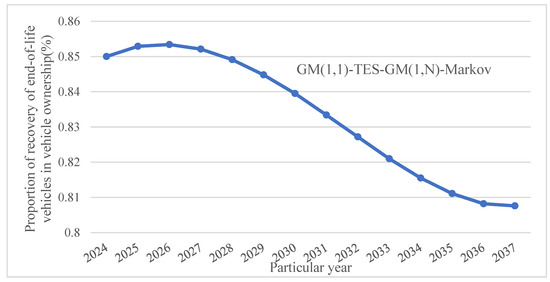
Figure 6.
Proportion of recovery of ELVs in vehicle ownership from 2024 to 2037.
The historical data of car ownership in various cities in Jiangsu Province of China shows a linear trend, and the least-squares linear regression is used to predict the future trend, as shown in Figure 7.
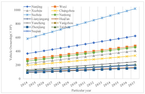
Figure 7.
Predicted number of car ownership from 2024 to 2037.
The number of ELVs recovered in the future can be calculated by Equation (46) below, and the ELV recovery quantity for each city in Jiangsu Province from 2024 to 2037 is shown in Figure 8.
where, is the number of ELVs recovered in city in the year, is the car ownership in city in the year, is the ratio of the number of ELVs recovered in China to the ownership of civilian vehicles in the year.
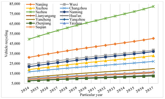
Figure 8.
The predicted values for the quantity of ELVs in Jiangsu Province from 2024 to 2037.
According to Equation (46), the predicted value of the number of ELVs recovered in various cities in Jiangsu Province from 2024 to 2037 can be obtained, as shown in Figure 8. According to GB/T 3730.1 “China Automobile Industry Yearbook [55]”, sedan cars, passenger cars, and trucks accounted for 41%, 35%, and 24% of the ELV recycling volume, respectively. Their average curb weights are 1.30 , 2.40 , and 4.50 , respectively. Taking 2032 as the planning year, the recovery quantities of different types of ELVs in Jiangsu Province and their corresponding triangular fuzzy numbers are obtained for that year, as shown in Table 8.
Table 8.
Recovery quantities of different types of ELVs in Jiangsu Province.
5.3. Optimization Results
- (1)
- Minimum total cost and the costs of each recycling process.
The minimum total cost of the base model is 667.49 million CNY. In an uncertain environment, the optimal solution of the objective function is and the total cost under this confidence level is 638.50 million CNY. The cost distribution of each recycling link is shown in Figure 9. Among them, the dismantling cost is the largest, followed by the machining cost. Compared to the basic model, the total cost of the network and the cost of each link in the uncertain environment are relatively low. This is because the basic model has strict constraints on the number of ELVs recovered, the handling capacity of the dismantling centers and the machining centers, which leads to an increase in the cost of each link. In the fuzzy model, the constraints of facility processing capacity and recycling quantity are looser.
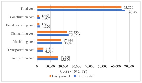
Figure 9.
The total cost and the costs of each recycling process.
- (2)
- Distribution of logistics between facilities.
In the uncertain environment, the distribution of logistics flow between nodes is shown in the figures below. In Figure 10, the three types of sedan cars, passenger cars, and trucks are separated by “/”, and the numbers represent the number of vehicles. The numbers in Figure 11 and Figure 12 represent the weight of materials transported between facilities.
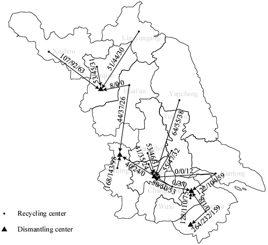
Figure 10.
Material flow distribution of various vehicle types from recycling center to dismantling center (×102 vehicles).
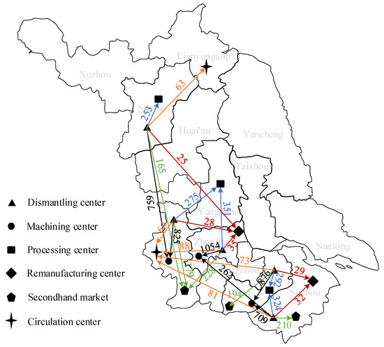
Figure 11.
Material flow distribution from dismantling center to each facility (×102 ton).
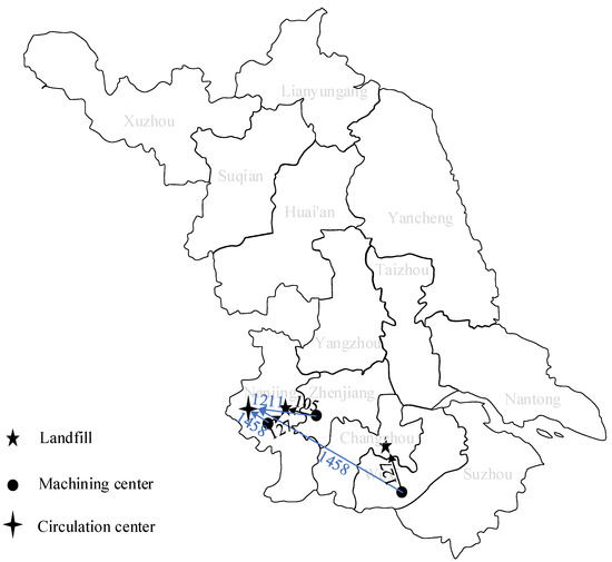
Figure 12.
Material flow distribution from the machining center to landfill plant and circulation center (×102 ton).
From the logistics distribution diagram, it can be seen that the optimal solution generated chooses to establish dismantling centers in five cities and machining centers in three cities. The facilities are distributed in the northern, central, and southern parts of Jiangsu Province, with denser distribution in the economically developed southern region, which can serve each city well.
5.4. Sensitivity Analysis
The sensitivity analysis of the model parameters, which observes their impact on costs, can provide support for managerial decision-making [56]. Changes in the number of ELVs recovered and the handling capacity of facilities will lead to different site selection results, as shown in Table 9. As the recycling volume increases, the total cost of the network also increases, along with the need for constructing more dismantling and machining centers. This is due to the current facilities being unable to keep up with the supply of ELVs for recycling. When the increase reaches 90%, due to the constraints of the number and handling capacity of dismantling and machining centers, there is no feasible solution; that is, not all ELVs can be recycled. At this time, increasing the handling capacity would lead to a feasible solution in the model. This would result in a reduction in the number of facilities, a change in the transportation plan, and ultimately a decrease in the total cost. The decline in total costs slows as the handling capacity increases because the handling capacity is far greater than the number of ELVs, and only the transportation scheme needs to be changed, without reducing the number of facilities. In addition, the impact of recycling volume on the total cost is greater than that of facility handling capacity, but the impact of both on the number of facility sites is similar. In this model, the construction cost of facilities is treated as an annual average construction cost. However, the actual initial investment in construction is substantial. The handling capacity of facilities directly affects the number of facilities to be constructed, and its impact cannot be ignored. Therefore, under the constraint of controlling the number of facilities, it is particularly important to construct a reverse logistics network when the recycling volume and facility processing capacity are uncertain. The research in this paper can provide a certain theoretical basis for decision-making.
Table 9.
Sensitivity analysis under fuzzy environment.
In contrast to sensitivity analysis conducted in a deterministic environment, this study assumes that the confidence level is an external parameter. The objective function is to minimize the total cost, and the study considers the optimal situation of the model under different confidence levels. The cost of each link and the locations of the dismantling and machining centers are shown in Table 10. When , the uncertainty of the model is the largest, and the total cost is 615.23 million CNY. When , the model is deterministic, the same as the base model. As the confidence level increases, the total cost increases approximately linearly, and the number of facilities required also increases. It can be observed that the increase in the number of facilities does not affect the construction location of facilities at lower confidence levels. Therefore, in cases where the number of facilities is limited, increasing the processing capacity of facilities can meet the recycling demand for ELVs. However, if the recycling demand is lower than expected, the excessive processing capacity of facilities will not be fully utilized. Therefore, the choice of confidence level has a critical impact on the rationality of the network layout. When formulating relevant regulations, the government should consult with enterprises to determine a reasonable confidence level.
Table 10.
Optimal solutions of models with different confidence levels.
6. Discussion
Reverse logistics can reintegrate waste materials into the production cycle for reuse, thereby reducing environmental pollution and resource waste. This is particularly crucial in the context of ELV recycling. The reverse logistics network further processes the recycled components and materials from ELVs through dismantling, sorting, processing, and recycling processes, thus creating a recyclable resource and generating new value. The reverse logistics network constructed in this study covers the entire process of ELV recycling, making site selection decisions for key facilities at each recycling stage. When designing the network, considering the uncertainties in real-world recycling can lead to a more rational layout.
The case analysis results reveal that, under uncertain conditions, there is a significant decrease in total network costs along with a reduction in the number of operational facilities. It is well understood that the number and location of facilities are strategic decisions that cannot be altered in the short term. Therefore, the construction quantity of facilities is high under certain conditions. However, if the actual ELV recycling quantity falls short of expectations, it will result in substantial capacity waste. Considering the uncertainties in recycling quantity and facility processing capacity, dynamic adjustment of facility processing capacity can be combined with actual recycling conditions. In situations where actual capacity fails to meet recycling demands, new facilities can be constructed in stages to ensure efficient resource utilization. The sensitivity analysis of the confidence level shows its significant impact on network design, where the confidence level represents the degree of uncertainty. Additionally, the sensitivity analysis of ELV recycling quantity and facility handling capacity demonstrates that the uncertainty in recycling quantity has a greater impact than the uncertainty in facility handling capacity. This is primarily because the recycling quantity decisively influences the number of facilities, site selection layout, transportation costs, processing costs, etc. Therefore, when decision-makers determine the planning scheme of the network, they need to make corresponding trade-offs based on different risk preferences and specific realities between system cost and reliability. It is advisable that the confidence level of the recycling quantity not be set too low.
The cost of facility handling accounts for a relatively high proportion of the total network cost. Enterprises can significantly reduce facility handling costs by developing and applying advanced and applicable technologies for recycling and reuse, thereby simultaneously reducing labor costs, management costs, time costs, and other related expenses. Therefore, it is recommended that government departments formulate laws and regulations related to the extension of producer responsibility for ELV recycling management in China. These laws should clarify the responsibilities of all parties involved and provide subsidies and rewards to outstanding individuals and enterprises. Additionally, creating an information sharing platform to facilitate information exchange between automotive and recycling enterprises, increasing the price of ELV recycling, and conducting specialized lectures on ELV recycling for the public can all help improve the recovery rate of ELVs through formal channels.
7. Conclusions
This paper firstly builds a grey–Markov combination model to predict the proportion of China’s ELV recycling to car ownership in the future years. According to the ratio of income and the number of vehicles in Jiangsu Province in the future year, obtained by the least square method, the number of ELVs recovered in each city in Jiangsu Province of China for future years is calculated. A multi-level ELV reverse logistics network is then constructed. To minimize the total cost, a MILP model is proposed. This model considers the recycling quantity of different types of ELVs, the proportion of different parts and materials, and the processing capacity of the facility. The complexity of the reverse logistics network model is increased, making the model more realistic. On this basis, a fuzzy programming model is proposed to maximize the expected level of fuzzy constraints, considering the uncertainty of the number of ELVs recovered and the facility’s processing capacity. The predicted vehicle ownership data of cities in Jiangsu Province of China are substituted into the model to verify the validity of the model.
The model proposed in this paper provides a quantitative method for solving the problem of ELV recycling in both certain and uncertain environments. It assists decision-makers in determining the optimal number and location of facilities to open, as well as the optimal transportation volume in the reverse logistics network. The results of this paper show that the dismantling center and the machining center have the largest handling cost in each link of the reverse logistics network. Changes in ELV recycling volumes and facility capacity have a greater impact on the overall cost and site selection. As the confidence level increases, the total cost increases approximately linearly, as does the number of facilities required. According to the model, when the actual recycling environment changes, decision-makers can identify an optimal recycling strategy. They can then rationally adjust the number and processing capacity of key facilities in the network based on actual demand. This can help reduce resource waste and environmental pollution caused by excess supply.
This study only considers the process of ELV recovery and designs an open-loop supply chain network. However, there is overlap among stakeholders involved in the entire automotive lifecycle. Further research could consider the entire life cycle from automobile sales to retirement, and design a closed-loop supply network with the objective of maximizing the sales profit of automobiles and recycled parts. Additionally, when analyzing large-scale cases, the number of variables and parameters involved in the model increases, making the solution process more complex. In such cases, developing heuristic algorithms to solve the model could be considered.
Author Contributions
Conceptualization, M.H. and T.L.; methodology, M.H., Q.L. and T.L.; software, Q.L. and T.L.; validation, M.H., J.F. and X.H.; formal analysis, Q.L.; investigation, T.L.; data curation, M.H.; writing—original draft preparation, M.H., Q.L. and T.L.; writing—review and editing, M.H. and Q.L.; visualization, Q.L. and J.F.; supervision, X.H. and X.W.; project administration, M.H.; funding acquisition, M.H. All authors have read and agreed to the published version of the manuscript.
Funding
This research was funded by the Opening Project of Intelligent Policing Key Laboratory of Sichuan Province (grant number No. ZNJW2023KFMS004).
Data Availability Statement
The original contributions presented in the study are included in the article, further inquiries can be directed to the corresponding authors.
Conflicts of Interest
The authors declare no conflicts of interest.
References
- Li, R.Y.M.; Du, H. Sustainable Construction Waste Management in Australia: A Motivation Perspective, Construction Safety and Waste Management: An Economic Analysis; Springer International Publishing: Cham, Switzerland, 2015; pp. 1–30. [Google Scholar]
- Stock, J.R. Reverse Logistics: White Paper; Council of Logistics Management: Oak Brook, IL, USA, 1992. [Google Scholar]
- Vermeulen, I.; Van Caneghem, J.; Block, C.; Baeyens, J.; Vandecasteele, C. Automotive shredder residue (ASR): Reviewing its production from end-of-life vehicles (ELVs) and its recycling, energy or chemicals’ valorisation. J. Hazard. Mater. 2011, 190, 8–27. [Google Scholar] [CrossRef]
- Nicolli, F.; Johnstone, N.; Söderholm, P. Resolving failures in recycling markets: The role of technological innovation. Environ. Econ. Policy Stud. 2012, 14, 261–288. [Google Scholar] [CrossRef]
- Wang, L.; Chen, M. Policies and perspective on end-of-life vehicles in China. J. Clean. Prod. 2013, 44, 168–176. [Google Scholar] [CrossRef]
- Analysis of the Scrap Motor Vehicle Recycling Situation in China from 2018 to 2022. Available online: https://huanbao.bjx.com.cn/news/20171117/862282.shtml (accessed on 4 March 2024).
- Premier Li Qiang Presided Over an Executive Meeting of the State Council: Actively Promote the Trade-In of Old Cars, Home Appliances, and Other Consumer Goods. Available online: https://baijiahao.baidu.com/s?id=1792522533173303807&wfr=spider&for=pc (accessed on 4 March 2024).
- Comprehensive Survey of the Scrap Car Recycling Industry. Available online: https://baijiahao.baidu.com/s?id=1705360000437264012&wfr=spider&for=pc (accessed on 4 March 2024).
- Li, R.Y.M.; Li, Y.L.; Crabbe, M.J.C.; Manta, O.; Shoaib, M. The Impact of Sustainability Awareness and Moral Values on Environmental Laws. Sustainability 2021, 13, 5882. [Google Scholar] [CrossRef]
- Choi, J.; Stuart, J.; Ramani, K. Modeling of automotive recycling planning in the United States. Int. J. Automot. Technol. 2005, 6, 413–419. [Google Scholar]
- Cruz-Rivera, R.; Ertel, J. Reverse logistics network design for the collection of End-of-Life Vehicles in Mexico. Eur. J. Oper. Res. 2009, 196, 930–939. [Google Scholar] [CrossRef]
- Demirel, E.; Demirel, N.; Gökçen, H. A mixed integer linear programming model to optimize reverse logistics activities of end-of-life vehicles in Turkey. J. Clean. Prod. 2016, 112, 2101–2113. [Google Scholar] [CrossRef]
- Özceylan, E.; Demirel, N.; Çetinkaya, C.; Demirel, E. A closed-loop supply chain network design for automotive industry in Turkey. Comput. Ind. Eng. 2017, 113, 727–745. [Google Scholar] [CrossRef]
- Phuc, P.N.K.; Yu, V.F.; Tsao, Y. Optimizing fuzzy reverse supply chain for end-of-life vehicles. Comput. Ind. Eng. 2017, 113, 757–765. [Google Scholar] [CrossRef]
- Simic, V.; Dimitrijevic, B. Interval linear programming model for long-term planning of vehicle recycling in the Republic of Serbia under uncertainty. Waste Manag. Res. 2015, 33, 114–129. [Google Scholar] [CrossRef]
- He, M.; Lin, T.; Wu, X.; Luo, J.; Peng, Y. A Systematic Literature Review of Reverse Logistics of End-of-Life Vehicles: Bibliometric Analysis and Research Trend. Energies 2020, 13, 5586. [Google Scholar] [CrossRef]
- Simic, V. Fuzzy risk explicit interval linear programming model for end-of-life vehicle recycling planning in the EU. Waste Manag. 2015, 35, 265–282. [Google Scholar] [CrossRef]
- Zhang, J.; Liu, J.; Wan, Z. Optimizing transportation network of recovering end-of-life vehicles by compromising program in polymorphic uncertain environment. J. Adv. Transp. 2019, 2019, 3894064. [Google Scholar] [CrossRef]
- Kuşakcı, A.O.; Ayvaz, B.; Cin, E.; Aydın, N. Optimization of reverse logistics network of End of Life Vehicles under fuzzy supply: A case study for Istanbul Metropolitan Area. J. Clean. Prod. 2019, 215, 1036–1051. [Google Scholar] [CrossRef]
- Xiao, Z.; Sun, J.; Shu, W.; Wang, T. Location-allocation problem of reverse logistics for end-of-life vehicles based on the measurement of carbon emissions. Comput. Ind. Eng. 2019, 127, 169–181. [Google Scholar] [CrossRef]
- Zarei, M.; Mansour, S.; Husseinzadeh Kashan, A.; Karimi, B. Designing a Reverse Logistics Network for End-of-Life Vehicles Recovery. Math. Probl. Eng. 2010, 2010, 649028. [Google Scholar] [CrossRef]
- Vidovic, M.; Dimitrijevic, B.; Ratkovic, B.; Simic, V. A novel covering approach to positioning ELV collection points. Resour. Conserv. Recycl. 2011, 57, 1–9. [Google Scholar] [CrossRef]
- Farel, R.; Yannou, B.; Bertoluci, G. Finding best practices for automotive glazing recycling: A network optimization model. J. Clean. Prod. 2013, 52, 446–461. [Google Scholar] [CrossRef]
- Gołębiewski, B.; Trajer, J.; Jaros, M.; Winiczenko, R. Modelling of the location of vehicle recycling facilities: A case study in Poland. Resour. Conserv. Recycl. 2013, 80, 10–20. [Google Scholar] [CrossRef]
- Simic, V. Interval-parameter chance-constraint programming model for end-of-life vehicles management under rigorous environmental regulations. Waste Manag. 2016, 52, 180–192. [Google Scholar] [CrossRef]
- Lin, Y.; Jia, H.; Yang, Y.; Tian, G.; Tao, F.; Ling, L. An improved artificial bee colony for facility location allocation problem of end-of-life vehicles recovery network. J. Clean. Prod. 2018, 205, 134–144. [Google Scholar] [CrossRef]
- Sun, Y.; Wang, Y.T.; Chen, C.; Yu, B. Optimization of a regional distribution center location for parts of end-of-life vehicles. Simulation 2018, 94, 577–591. [Google Scholar] [CrossRef]
- Budak, A. Sustainable reverse logistics optimization with triple bottom line approach: An integration of disassembly line balancing. J. Clean. Prod. 2020, 270, 122475. [Google Scholar] [CrossRef]
- Govindan, K.; Gholizadeh, H. Robust network design for sustainable-resilient reverse logistics network using big data: A case study of end-of-life vehicles. Transp. Res. Part E Logist. Transp. Rev. 2021, 149, 102279. [Google Scholar] [CrossRef]
- Hashemi, S.E. A fuzzy multi-objective optimization model for a sustainable reverse logistics network design of municipal waste-collecting considering the reduction of emissions. J. Clean. Prod. 2021, 318, 128577. [Google Scholar] [CrossRef]
- Shafiee Roudbari, E.; Fatemi Ghomi, S.M.T.; Sajadieh, M.S. Reverse logistics network design for product reuse, remanufacturing, recycling and refurbishing under uncertainty. J. Manuf. Syst. 2021, 60, 473–486. [Google Scholar] [CrossRef]
- Wenzhu Liao, G.H.; Luo, X. Collaborative reverse logistics network for electric vehicle batteries management from sustainable perspective. J. Environ. Manag. 2022, 324, 116352. [Google Scholar] [CrossRef] [PubMed]
- Reddy, K.N.; Kumar, A.; Choudhary, A.; Cheng, T.C.E. Multi-period green reverse logistics network design: An improved Benders-decomposition-based heuristic approach. Eur. J. Oper. Res. 2022, 303, 735–752. [Google Scholar] [CrossRef]
- Kannan, D.; Solanki, R.; Darbari, J.D.; Govindan, K.; Jha, P.C. A novel bi-objective optimization model for an eco-efficient reverse logistics network design configuration. J. Clean. Prod. 2023, 394, 136357. [Google Scholar] [CrossRef]
- Ene, S.; Öztürk, N. Network modeling for reverse flows of end-of-life vehicles. Waste Manag. 2015, 38, 284–296. [Google Scholar] [CrossRef]
- Ahmed, A.; Ali, D. A Reverse Logistics Network Design. J. Manuf. Syst. 2015, 37, 589–598. [Google Scholar]
- Govindan, K.; Paam, P.; Abtahi, A. A fuzzy multi-objective optimization model for sustainable reverse logistics network design. Ecol. Indic. 2016, 67, 753–768. [Google Scholar] [CrossRef]
- Yi, P.; Huang, M.; Guo, L.; Shi, T. A retailer oriented closed-loop supply chain network design for end of life construction machinery remanufacturing. J. Clean. Prod. 2016, 124, 191–203. [Google Scholar] [CrossRef]
- Rodolfo, G.; Carlos, A. Operational Planning of Forward and Reverse Logistic Activities on Multi-echelon Supply-chain Networks. Comput. Chem. Eng. 2016, 88, 170–184. [Google Scholar]
- Kumar, V.N.S.A.; Kumar, V.; Brady, M.; Garza-Reyes, J.A.; Simpson, M. Resolving forward-reverse logistics multi-period model using evolutionary algorithms. Int. J. Prod. Econ. 2017, 183, 458–469. [Google Scholar] [CrossRef]
- Simic, V. A two-stage interval-stochastic programming model for planning end-of-life vehicles allocation under uncertainty. Resour. Conserv. Recycl. 2015, 98, 19–29. [Google Scholar] [CrossRef]
- Simic, V. A multi-stage interval-stochastic programming model for planning end-of-life vehicles allocation. J. Clean. Prod. 2016, 115, 366–381. [Google Scholar] [CrossRef]
- Ene, S.; Öztürk, N. Grey modelling based forecasting system for return flow of end-of-life vehicles. Technol. Forecast. Soc. Chang. 2017, 115, 155–166. [Google Scholar] [CrossRef]
- Soki, M.D.; Ili, I.B.; Manojlovi, V.D.; Markovi, B.R.; Trbac, N.D. Modeling and Prediction of the end of Life Vehicles Number Distribution in Serbia. Acta Polytech. Hung. 2016, 13, 2016–2159. [Google Scholar] [CrossRef]
- Xin, F.; Ni, S.; Li, H.; Zhou, X. General Regression Neural Network and Artificial-Bee-Colony Based General Regression Neural Network Approaches to the Number of End-of-Life Vehicles in China. IEEE Access 2018, 6, 19278–19286. [Google Scholar] [CrossRef]
- Yi Man Li, R.; Song, L.; Li, B.; James, C.; Crabbe, M.; Yue, X. Predicting Carpark Prices Indices in Hong Kong Using AutoML. Comput. Model. Eng. Sci. 2023, 134, 2247–2282. [Google Scholar] [CrossRef]
- Yu, L.; Chen, M.; Yang, B. Recycling policy and statistical model of end-of-life vehicles in China. Waste Manag. Res. 2019, 37, 347–356. [Google Scholar] [CrossRef] [PubMed]
- Zhang, J.; Gao, M.; Zhao, L.; Hu, J.; Gao, J.; Deng, M.; Wan, C.; Yang, L. Multi-time Scale Attention Network for WEEE reverse logistics return prediction. Expert Syst. Appl. 2023, 211, 118610. [Google Scholar] [CrossRef]
- Batool, N.; Hussain, S.; Kausar, N.; Munir, M.; Li, R.Y.M.; Khan, S. Intuitionistic multi fuzzy ideals of near-rings. Decis. Mak. Appl. Manag. Eng. 2023, 6, 564–582. [Google Scholar] [CrossRef]
- Deng, J. Grey Theory Foundation; Huazhong University of Science and Technology Press: Wuhan, China, 2002. [Google Scholar]
- Yao, Y.; Wang, J.; Zhou, Z.; Li, H.; Liu, H.; Li, T. Grey Markov prediction-based hierarchical model predictive control energy management for fuel cell/battery hybrid unmanned aerial vehicles. Energy 2023, 262, 125405. [Google Scholar] [CrossRef]
- Jiang, X.; Chen, S. Application of Weighted Markov SCGM(1,1) c Model to Predict Drought Crop Area. Syst. Eng. 2009, 29, 179–185. [Google Scholar] [CrossRef]
- Michaliszyn, J.; Otop, J. Non-deterministic weighted automata evaluated over Markov chains. J. Comput. Syst. Sci. 2020, 108, 118–136. [Google Scholar] [CrossRef]
- Zhumadillayeva, A.; Orazbayev, B.; Santeyeva, S.; Dyussekeyev, K.; Li, R.Y.M.; Crabbe, M.J.C.; Yue, X. Models for Oil Refinery Waste Management Using Determined and Fuzzy Conditions. Information 2020, 11, 299. [Google Scholar] [CrossRef]
- CATARC; CAAM. China Automotive Industry Yearbook; China Automotive Industry Yearbook Journal Society: Tianjin, China, 2022.
- Shi, Y.; Lin, Y.; Li, B.; Li, R.Y.M. A bi-objective optimization model for the medical supplies’ simultaneous pickup and delivery with drones. Comput. Ind. Eng. 2022, 171, 108389. [Google Scholar] [CrossRef]
Disclaimer/Publisher’s Note: The statements, opinions and data contained in all publications are solely those of the individual author(s) and contributor(s) and not of MDPI and/or the editor(s). MDPI and/or the editor(s) disclaim responsibility for any injury to people or property resulting from any ideas, methods, instructions or products referred to in the content. |
© 2024 by the authors. Licensee MDPI, Basel, Switzerland. This article is an open access article distributed under the terms and conditions of the Creative Commons Attribution (CC BY) license (https://creativecommons.org/licenses/by/4.0/).